Global Sensitivity Analysis of Uncertain Parameters in Bayesian Networks

Abstract

Traditionally, the sensitivity analysis of a Bayesian network studies the impact of individually modifying the entries of its conditional probability tables in a one-at-a-time (OAT) fashion. However, this approach fails to give a comprehensive account of each inputs’ relevance, since simultaneous perturbations in two or more parameters often entail higher-order effects that cannot be captured by an OAT analysis. We propose to conduct global variance-based sensitivity analysis instead, whereby $n$ parameters are viewed as uncertain at once and their importance is assessed jointly. Our method works by encoding the uncertainties as $n$ additional variables of the network. To prevent the curse of dimensionality while adding these dimensions, we use low-rank tensor decomposition to break down the new potentials into smaller factors. Last, we apply the method of Sobol to the resulting network to obtain $n$ global sensitivity indices. Using a benchmark array of both expert-elicited and learned Bayesian networks, we demonstrate that the Sobol indices can significantly differ from the OAT indices, thus revealing the true influence of uncertain parameters and their interactions.

organization=School of Science and Technology, IE University,city=Madrid, country=Spain

1 Introduction

Amongst the many machine learning methods now available to practitioners, Bayesian networks (BNs) are undoubtedly one of the most widespread due to their interpretability, ease of modelling, and wide array of software available (Koller et al., 2009; Pearl, 1988). BNs consist of a directed acyclic graph expressing the dependence relationship between the variables of interest, and one-dimensional conditional probability distributions from which various inferential queries can be answered. There are now uncountable applications of such models in a wide array of domains (e.g. Bielza and Larrañaga, 2014; Drury et al., 2017; Hosseini and Ivanov, 2020; Kabir and Papadopoulos, 2019; Marcot and Penman, 2019; McLachlan et al., 2020). One of the main strengths of BNs is that they cannot only be learned from data, but they can also be expert-elicited, both in the structure of its underlying graph and its associated probabilities (Barons et al., 2022).

A fundamental but sometimes overlooked aspect of any real-world BN analysis is the robustness of outputs of interest w.r.t. misspecification of the model probabilities. In the field of BNs, this type of investigation is usually referred to as parametric sensitivity analysis (Rohmer, 2020), and its use has recently become more popular (e.g. Giles et al., 2023; Jindal et al., 2022; Ma et al., 2022; Wang et al., 2023).

The functional relationship between outputs and the BN model probabilities has been extensively studied in the literature (Castillo et al., 1997; Coupé and Van Der Gaag, 2002; Laskey, 1995; Rohmer and Gehl, 2020; Van Der Gaag et al., 2007). However, as Rohmer (2020) has noted, most approaches that have been studied fall under the umbrella of one-at-a-time (OAT) sensitivity analysis or one-way sensitivity analysis. OAT investigates the effect of local variations to one parameter only while keeping the rest fixed, thus providing only a partial picture of the system’s robustness. Attempts to vary more than one parameter at a time, the so-called multi-way sensitivity analysis approach (Bolt and Renooij, 2014; Bolt and van der Gaag, 2017; Kjærulff and van der Gaag, 2000; Leonelli et al., 2017), quickly become computationally infeasible for most real-world BNs (Chan and Darwiche, 2004; Kwisthout and van der Gaag, 2008; Leonelli and Riccomagno, 2022), although some recent technical advances that map BNs to Markov chains or tensor networks (TNs) have been exploited to speed up computations (Ballester-Ripoll and Leonelli, 2023; Salmani and Katoen, 2021, 2023a, 2023b).

Outside BNs, the most common approach is the so-called global sensitivity analysis (Saltelli et al., 2000, 2008), which provides a “global”, instead of local, representation of how different factors jointly influence some function of the model’s output. As noticed by Saltelli et al. (2021), global sensitivity is en route to becoming an integral part of mathematical modelling. Its tremendous potential benefits are yet to be fully realized, both for advancing data-driven modelling of human and natural systems and in supporting decision-making (Razavi et al., 2021). Furthermore, the latest trends in machine learning focus on models whose workings can be interpreted and explained (explainable artificial intelligence, or XAI), and sensitivity analysis plays a central role in this task (Linardatos et al., 2020; Van Stein et al., 2022).

To our knowledge, there have been only three recent attempts to implement global sensitivity methods for BNs. Li and Mahadevan (2017) and Zio et al. (2022) implemented Monte Carlo-based estimation routines for global sensitivity indices. However, their approach suffers from two significant drawbacks: it is infeasible for moderate-size networks since it is based on a very complex Monte Carlo simulation; their implementation is not freely available, and therefore, other practitioners cannot utilize the routines in their work. Ballester-Ripoll and Leonelli (2022a) implemented global sensitivity analysis techniques in BNs and developed exact methods for their computation based on TNs. Still, all these methods address the so-called sensitivity to evidence problem (e.g. Gómez-Villegas et al., 2014), which identifies the most informative evidence that could be observed to improve the assessment of the output of interest.

In this paper, we develop algorithms for the computation of global sensitivity indexes for parametric (as opposed to evidential) sensitivity analyses in BNs. To this end, we leverage the duality between probabilistic graphical models and TNs (Robeva and Seigal, 2018). By first representing BNs as Markov random fields (MRFs) and then as TNs, the approach utilizes the duality between these representations to facilitate complex computations. This transformation allows for the application of sophisticated tensor operations, which are critical for handling the high-dimensional structures inherent in BNs. Specifically, the Sobol index computation is achieved through element-wise product operations followed by tensor contraction, enabling a more comprehensive sensitivity analysis that accounts for interactions between parameters.

More specifically, the proposed method augments tensors in a novel way, embedding uncertainties directly into the tensor structures. This augmentation, while potentially leading to computational infeasibility due to the increased dimensionality, is managed by employing state-of-the-art tensor contraction and manipulation libraries. These tools, particularly tensor train decompositions (Oseledets, 2011), allow for efficient processing by breaking down tensors into smaller, more manageable components. This decomposition not only mitigates the computational burden but also preserves the integrity of the sensitivity analysis, making it feasible to handle large and complex networks.

In short, we develop a novel algorithmic solution for the interpretability of these machine learning models, providing a significant advance in knowledge and an impactful tool for applied analyses in many areas of science. This is particularly critical given that often ad-hoc solutions are implemented which may lead to false conclusions as observed by Do and Razavi (2020) and Saltelli et al. (2019). In this paper, we showcase the method (and the insights it provides in practice) using a real-world application on the consequences of the COVID-19 pandemic at the European level.

2 Background

2.1 Bayesian Networks

Consider a categorical random vector of interest $\bm{Y}=(Y_{1},\dots,Y_{p})$. A BN gives a graphical representation of the relationship between the variables $\bm{Y}$ using a directed acyclic graph and a factorization of the overall probability distribution $P(\bm{Y}=\bm{y})$, where $\bm{y}$ is an element of the sample space $\mathbb{Y}=\times_{i\in\{1,\dots,p\}}\mathbb{Y}_{i}$, in terms of simpler conditional distributions $P(Y_{i}=y_{i}|\bm{Y}_{\Pi_{i}}=\bm{y}_{\Pi_{i}})$, where $\bm{Y}_{\Pi_{i}}$ denotes the parents of $Y_{i}$. More formally, the overall factorization of the probability distribution induced by the BN can be written as:

$$P(\bm{Y}=\bm{y})=\prod_{i=1}^{p}P(Y_{i}=y_{i}|\bm{Y}_{\Pi_{i}}=\bm{y}_{\Pi_{i}})$$

Figure 1 gives an example of a simple BN. The nodes are the variables of the problems and the arcs represent direct dependence relationships. The lack of an arc formally represents conditional independence as formalized by the d-separation criterion of Pearl (2009). BNs, giving a graphical representation of the structure of the mathematical model, are particularly suited for applied analyses since they can be interpreted and understood having little, if no, previous mathematical knowledge.

$Y_{1}$
no	yes
0.60	0.40
$Y_{2}$
no	yes
0.70	0.30

		$Y_{3}$
$Y_{1}$	$Y_{2}$	no	yes
no	no	0.70	0.30
no	yes	0.60	0.40
yes	no	0.60	0.40
yes	yes	0.05	0.95

Figure 1: An example of a DAG over three binary random variables $Y_{1},Y_{2},Y_{3}$ with the associated probability specifications $\bm{\theta}^{0}$.

The conditional probabilities $P(Y_{i}=y_{i}|\bm{Y}_{\Pi_{i}}=\bm{y}_{\Pi_{i}})$ defining the BN model are usually denoted as $\bm{\theta}$ and, for categorical variables, form the so-called conditional probability tables (CPTs). The CPTs are either learned from data using machine learning algorithms (Scutari et al., 2019) or expert-elicited through probability elicitation exercises (Barons et al., 2022). No matter the method used, we assume a value for the probabilities $\bm{\theta}$ has been chosen, which we refer to as the original value and denote as $\bm{\theta}^{0}$. For our simple example, these are reported on the right-hand side of Figure 1. Because of imprecisions during elicitation or low quality of observed data, it is imperative to check the effect of potential perturbations of $\bm{\theta}^{0}$ on the output of the BN model. This assessment is carried out via sensitivity analysis.

2.2 Parametric Sensitivity Analysis in BNs

We henceforth consider the conditional probabilities $\bm{\theta}$ defining the model as our objects of study. Let $Y_{O}$ be an output variable of interest and consider the probability of interest $f_{O}(\bm{\theta})=P(Y_{O}=y_{O})$ for some level $y_{O}$. Seen as a function of a chosen vector of conditional probabilities $\bm{\theta}$, $f$ is called a sensitivity function (Van Der Gaag et al., 2007).

Consider the BN in Figure 1 and suppose $Y_{1}$ and $Y_{2}$ describe two medical tests that could be either positive or negative, while $Y_{3}$ is the presence of a specific disease. Suppose our output of interest is $P(Y_{3}=\textnormal{yes})$, the probability that an individual has the disease. In Figure 2, we report the one-way sensitivity functions associated with the probability that a test is positive, constructed using the bnmonitor R package (Leonelli et al., 2023). It can be clearly seen that individually, the two parameters have a very limited effect on the output probability, which changes very slowly as the parameter of interest is varied.

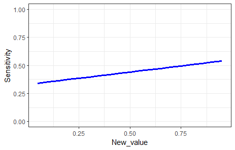
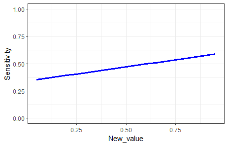
Figure 2: Sensitivity functions for the output probability $P(Y_{3}=\textnormal{yes})$ as a function of $P(Y_{1}=\textnormal{yes})$ (left) and $P(Y_{2}=\textnormal{yes})$ (right).

A standard way to summarize one-way sensitivity functions is by considering the gradient at the original value of the considered parameter $\theta_{i}^{0}$. More formally, the $i$-th sensitivity value is usually reported and formally defined as $|f^{\prime}_{O}(\theta_{i}^{0})|$. For the two sensitivity functions in Figure 2, these values can be either computed manually using standard probability derivations or using an exact method such as YODO (Ballester-Ripoll and Leonelli, 2022b). They are very small in this case: 0.015 and 0.060, respectively.

2.3 Proportional Covariation

After the variation of an input $\theta_{i}$ from its original value $\theta_{i}^{0}$ the sum-to-one condition of probabilities does not hold anymore. For this reason, parameters from the same conditional distribution are covaried to respect this constraint. When variables are binary, this is automatic since one parameter must be equal to one minus the other. When variables are categorical with more than two levels, there are multiple methods to covary parameters (Renooij, 2014). Proportional covariation (Laskey, 1995) is the gold-standard method since it is motivated by a wide array of theoretical properties (Chan and Darwiche, 2005; Leonelli et al., 2017; Leonelli and Riccomagno, 2022). When a parameter $\theta_{j}$ from the same conditional distribution of the varied parameter $\theta_{i}$ is proportionally covaried it equals:

$$\theta_{j}(\theta_{i})=\frac{1-\theta_{i}}{1-\theta^{0}_{i}}\theta^{0}_{j}.$$

Under the assumption of proportional covariation, Castillo et al. (1997) and Coupé et al. (2000) proved that the sensitivity function equals the ratio of two linear functions:

$$f(\theta_{i})=\frac{c_{0}+c_{i}\theta_{i}}{d_{0}+d_{i}\theta_{i}},$$

where $c_{0},c_{i},d_{0},d_{i}\in\mathbb{R}$.

2.4 Motivating Example: Limitation of OAT Methods

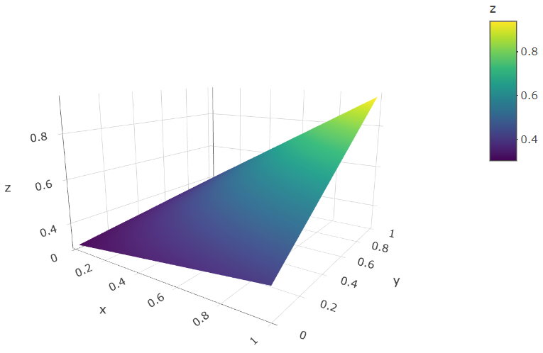
Figure 3: Two-way sensitivity function for $P(Y_{3}=\textnormal{yes})$ as a function of $P(Y_{1}=\textnormal{yes})$ and $P(Y_{2}=\textnormal{yes})$.

It is well known that OAT sensitivity methods only provide a partial and sometimes wrong picture of the influence of the input parameters (Saltelli et al., 2019). Our simple BN example in Figure 1 illustrates this. Consider now the probability of having the disease $P(Y_{3}=\textnormal{yes})$ as a function of the two tests being positive $P(Y_{1}=\textnormal{yes})$ and $P(Y_{2}=\textnormal{yes})$. Figure 3 reports this probability as a function of both parameters. It can be clearly seen there is a steep increase in the probability of having the disease when the probability of both tests being positive increases. On the other hand, the two parameters individually have a minor impact on the output probability, as already noticed in Figure 2. To draw a parallelism, this is similar to a two-way ANOVA when there is a strong interaction term between the two factors. Of course, this example is trivial and the joint effect of both parameters could have been already noticed by simply looking at the conditional probabilities in Figure 1. Still, it illustrates the limitation of OAT analyses in BNs even in the simplest scenario.

In the context of BNs, multi-way sensitivity analyses where multiple parameters are varied simultaneosly have been studied. However, their computation and interpretation becomes challenging. We can notice that (i) sensitivity functions cannot be visualized in high dimensions; (ii) the number of groups of parameters that could be varied grows exponentially; (iii) most critically, the associated measures are challenging to interpret, similar to higher-order interactions in standard statistical models (see e.g. Hayes et al., 2012). For these reasons, we argue that a global approach is better suited to thoroughly investigate the effect of the parameters of a BN model.

2.5 Sobol Indices

Sobol indices represent one of the most widely used frameworks for global sensitivity of a function $f:\Omega\subseteq\mathbb{R}^{n}\rightarrow\mathbb{R}$ taking values in a $n$-dimensional rectangle $\times_{i\in\{1,\dots,k\}}\Omega_{i}$ (Sobol, 1990). Although there are many different types of indices, for our purposes we focus on two of the most common ones, namely the variance component and the total index.

Henceforth, consider a $n$-dimensional vector $\bm{\theta}=(\theta_{1},\dots,\theta_{n})$ of input parameters, whose uncertainty needs to be assessed. The variance component associated to $\theta_{i}$ is

$$S_{i}:=\frac{\mathrm{Var}_{i}\left[\textnormal{E}_{\setminus i}[f]\right]}{\mathrm{Var}[f]},$$ (1)

where $\textnormal{E}_{\setminus i}$ is the expectation with respect to $\boldsymbol{\theta}_{\setminus i}$ and $\mathrm{Var}_{i}$ is the variance with respect to $\theta_{i}$. The variance component quantifies how the average model output changes as $\theta_{i}$ is varied. In other words, it is an additive measure over $\theta_{i}$.

The total index of the parameter $\theta_{i}$ swaps the roles of the expectation and the variance in Eq. (1):

$$S^{T}_{i}:=\frac{\textnormal{E}_{\setminus i}\left[\mathrm{Var}_{i}[f]\right]}{\mathrm{Var}[f]}.$$

The total index quantifies the average variability in the model output due to changes in $\theta_{i}$ only. Compared to the variance component, the total index is an overall measure, which includes additive effects but also interaction terms. Thus, $S_{i}\leq S^{T}_{i}$. The two indices are equal if and only if $f(\boldsymbol{\theta})=g(\theta_{i})+h(\boldsymbol{\theta}_{\setminus i})$, that is if $\theta_{i}$ can be separated from $f$ in an additive fashion. Among other uses, total indices are a popular tool for model simplification: whenever a model input $\theta_{i}$ has a small $S^{T}_{i}$, it can be safely fixed to any reasonable constant, thus decreasing the degrees of freedom.

2.6 Tensor Train Decomposition

The tensor train low-rank decomposition (Oseledets, 2011), or TT for short, factorizes a high-dimensional tensor into a linear network of tensors that are at most three-dimensional. If $\mathcal{T}$ is a tensor of shape $I_{1}\times\dots\times I_{N}$, the TT format approximates it as

$$\mathcal{T}(i_{1},\dots,i_{N})\approx G_{1}(i_{1})\cdots G_{N}(i_{N})$$ (2)

where $G_{1}(i_{1})$ is a row vector, $G_{2}(i_{2}),\dots,G_{N-1}(i_{N-1})$ are matrices, and $G_{N}(i_{N})$ is a column vector for any values $1\leq i_{1}\leq I_{1},\dots,1\leq i_{N}\leq I_{N}$.

We can use this format to break up CPTs into smaller tensors, thus decreasing their number of degrees of freedom. For example, a node $A$ with three parents $B,C,D$ will have a CPT $\Phi$ of 4 dimensions. Viewed as a tensor, it can be written in the TT format as

$$\Phi(y_{A},y_{B},y_{C},y_{D})\approx\sum_{r_{1},r_{2},r_{3},r_{4}}G_{1}(y_{A},r_{1})G_{2}(r_{1},y_{B},r_{2})G_{3}(r_{2},y_{C},r_{3})G_{4}(r_{3},y_{D})$$ (3)

where the $r_{1},\dots,r_{N-1}$ are known as bond dimensions (or TT ranks) and play the role of latent variables. The model reduction induced by the TT format comes at the expense of a variable compression error $\epsilon$. In any case, that error may be reduced by increasing $\boldsymbol{r}$ as necessary, and $\epsilon$ can be even brought to zero when the tensor is exactly low-rank.

Note that directly compressing a CPT as in Eq. (3) is rarely useful. A more common use of low-rank decompositions in this context is to apply truncated singular value decomposition (SVD) to break up intermediate factors during tensor contraction (Gray and Chan, 2024) (which is equivalent to variable elimination in exact BN inference). In this paper, we will use the TT format to handle “enriched” CPTs that incorporate additional degrees of freedom due to parametric uncertainties in the BN. In practice, we will use the following variant of Eq. (2):

$$\mathcal{T}(i_{1},\dots,i_{N})\approx(G_{1}\times_{2}\mathbf{U}_{1})(i_{1})\cdots(G_{N}\times_{2}\mathbf{U}_{N})(i_{N})$$ (4)

where the $\times_{2}$ is the tensor-times-matrix product along the second mode (Kolda and Bader, 2009) and the $\mathbf{U}_{1},\dots,\mathbf{U}_{N}$ are learned matrices that provide a convenient extra level of compression when dimensions represent continuous variables (as is the case for our uncertainties). Although Eq. (4) has sometimes been called extended tensor train in the literature (Schneider and Uschmajew, 2014), we will simply refer to it as TT in this paper.

3 The Algorithm

Our goal is to apply Sobol’s method to address the limitations of OAT parametric sensitivity analyses in BNs illustrated in Section 2.4. For simplicity, we will refer to all probability tables in the model as CPTs even when a node has no parents. Our algorithm takes a BN and a list of uncertain CPT entries $\bm{\theta}$ and produces a Sobol index for each $\theta_{i}$. It consists of four steps:

1. We moralize the BN and interpret it as a tensor network.

2. For each CPT that includes uncertain entries, we encode each uncertainty as an additional new parent (i.e., a new dimension of the CPT).

3. To avoid exponential blow-up of the augmented CPTs, we compactly encode them using a low-rank TT decomposition. Within the broader network, we seamlessly replace the original affected CPTs for their TT versions. For computational efficiency reasons, we execute this step at the same time as the previous one.

4. Using the method of Sobol, we extract sensitivity indices of the resulting TN for the set of added new variables. We use the algorithm of Ballester-Ripoll and Leonelli (2022a) with exact inference for this step.

Next, we detail each step in depth.

3.1 Moralization and Conversion to a Tensor Network

Graph moralization is a standard step for casting a BN into a Markov random field (MRF) (e.g. Koller et al., 2009). It involves two steps:

1. Removing all arrow directions.

2. Connecting (marrying) each pair of parents together, so that each CPT for a node with $k$ parents becomes a clique of $(k+1)$ nodes with an associated $(k+1)$-dimensional potential.

Furthermore, in this paper we represent MRFs as tensor networks (TNs). The TN formulation is equivalent to that of MRFs (Robeva and Seigal, 2018), since each one is the dual graph of the other:

• The nodes of an MRF become edges (or hyperedges, if the node has three or more neighbors) in the TN.

• The edges (network cliques are counted as hyperedges) of an MRF become nodes in the TN. The tensors in the TN are simply the MRF potentials.

See Figure 4 for an example of moralization and conversion to TN by means of the dual graph.

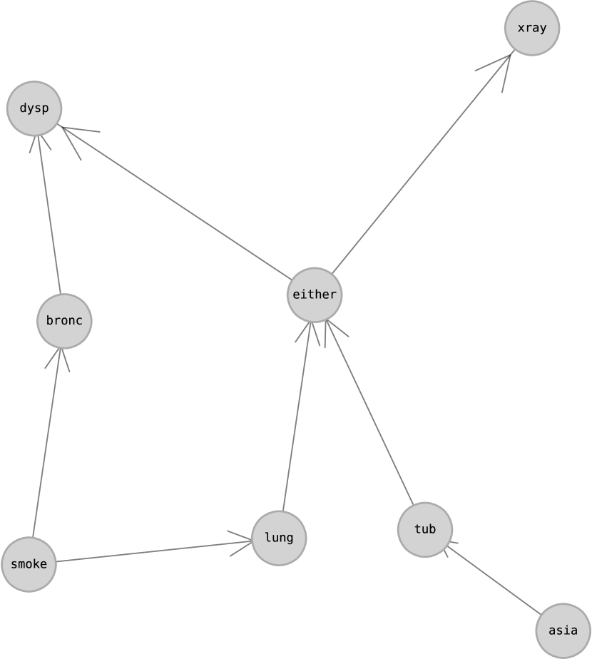
(a) An input Bayesian network $\mathcal{B}$.

(b) MRF $\mathcal{M}$ that results from moralizing $\mathcal{B}$.

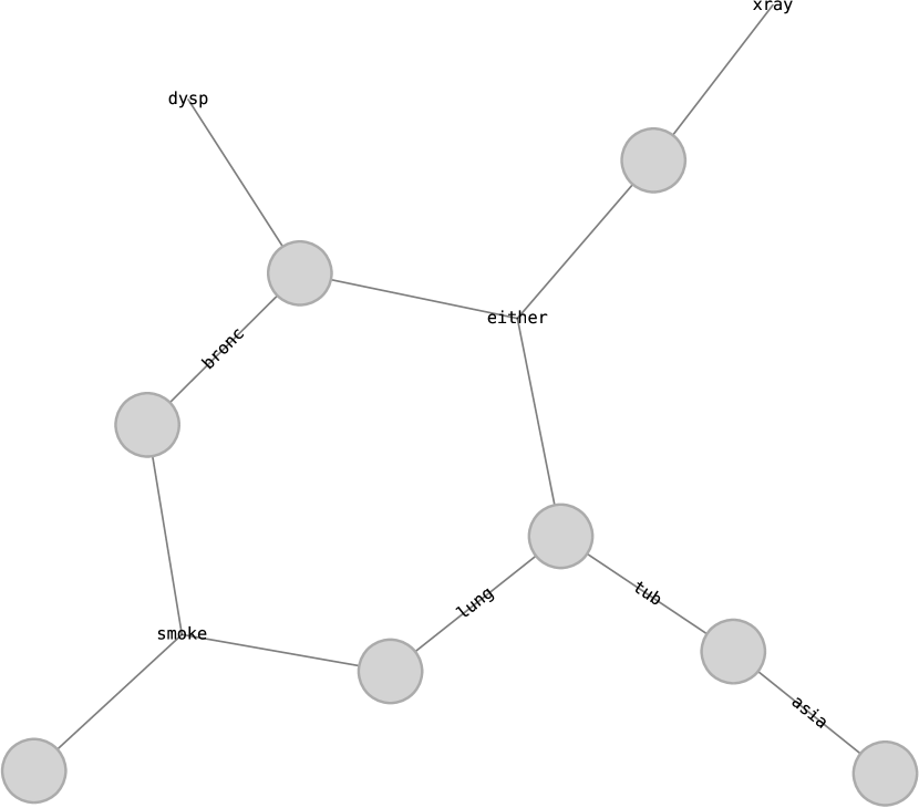
(c) Tensor network representation (dual of (b)).

Figure 4: The asia network as a Bayesian network (a), Markov random field (b), and tensor network (c). Note that, if the cliques of (b) are regarded as hyperedges, then (c) is the dual graph of (b).

The TN representation makes it easier to illustrate the “surgical” network manipulation operations we perform in later steps, since the low-rank decomposition we use (tensor train) is usually represented as a TN in the literature.

3.2 Encoding Uncertainties

Let the CPT for variable $Y$ with parents $\bm{Y}_{\Pi}$ be denoted as $\Phi(Y=y,\bm{Y}_{\Pi}=\bm{y}_{\Pi})$. Let us assume we have $P$ uncertain entries in $\Phi$, with $y_{1},\dots,y_{P}$ denoting the child and $\boldsymbol{y}_{1}^{\mathbb{U}},\dots,\boldsymbol{y}_{P}^{\mathbb{U}}$ denoting the parent indices of those entries. As an example, if the uncertain entries in the CPT of a node $A$ are $\{P(A=1|B=0,C=0),P(A=1|B=1,C=1)$, then $y_{1}=1,y_{2}=1,\bm{y}_{1}^{\mathbb{U}}=(0,0),\bm{y}_{2}^{\mathbb{U}}=(1,1)$. Note that we do not support multiple uncertain entries for a single parent configuration, i.e. $\boldsymbol{y}_{a}^{\mathbb{U}}\neq\boldsymbol{y}_{b}^{\mathbb{U}}$ for all $a\neq b$. The reason is that the constraint $\sum_{y}\Phi(Y=y,\bm{Y}_{\Pi}=\bm{y}_{\Pi})=1$ imposes a relationship between these entries, making them correlated and hence unsuitable for a Sobol analysis.

Our goal is to build an “augmented” potential $\Phi^{\prime}$ that includes new dimensions $x_{1},\dots,x_{P}$ with $x_{p}\in[0,1]$ for all $p$. Both $\Phi^{\prime}$ and $\Phi$ are identical (and the $x_{p}$ dummy) everywhere except on the uncertain indices. On each uncertain entry $p$, we have that $\Phi^{\prime}(\bm{x},y_{p},\bm{y}_{p}^{\mathbb{U}}):=x_{p}$, whereas entries of $\Phi^{\prime}$ for other child values $Y\neq y_{p}$ are adjusted accordingly using proportional covariation (Laskey, 1995). More compactly:

$$\Phi^{\prime}(\bm{X}=\bm{x},Y=k,\bm{Y}_{\Pi}=\bm{y}_{\Pi}):=$$

$$\begin{cases}\frac{1-x_{p}}{1-\Phi(y_{p},\bm{y}_{\Pi})}\Phi(k,\bm{y}_{\Pi})&\mbox{ if }\bm{y}_{\Pi}=\bm{y}_{p}^{\mathbb{U}}\mbox{ for some }p\in\{1,\dots,P\}\\ \Phi(k,\bm{y}_{\Pi})&\mbox{otherwise.}\end{cases}$$

The new tensor $\Phi^{\prime}$ has $P$ more dimensions than $\Phi$ and could become computationally intractable even at modest values of $P$. Fortunately, it can be succinctly represented in the TT format by virtue of the following lemma.

Lemma 1.

The potential $\Phi^{\prime}$ defined above has TT rank at most $\sqrt{|\Phi|}+P$, where $|\Phi|$ is the total number of elements of $\Phi$.

Proof.

Let us break down the augmented potential as $\Phi^{\prime}:=\Phi+\mathcal{T}_{1}+\dots\mathcal{T}_{P}$, where each $\mathcal{T}_{p}$ is a function defined as:

$$\mathcal{T}_{p}(\boldsymbol{x},y,\bm{y}_{\Pi}):=\begin{cases}\frac{1-x_{p}}{1-\Phi(y_{p},\bm{y}_{\Pi})}\Phi(k,\bm{y}_{\Pi})-\Phi(k,\bm{y}_{\Pi})&\mbox{ if }\bm{y}_{\Pi}=\bm{y}_{p}^{\mathbb{U}}\\ 0&\mbox{otherwise.}\end{cases}$$ (5)

Essentially, Eq. (5) replaces the original distribution $\Phi(Y=k)$ for $k=1,\dots,|Y|$ by subtracting it and adding its proportionally covaried version instead; in other words, it ensures the new distribution still sums to 1 for all values of $x_{p}$ in $[0,1]$.

Next, let us see that $\mathcal{T}_{p}$ has TT rank 1 for any $p=1,\dots,P$. Its non-zero terms equal $\left(\frac{1-x_{p}}{1-\Phi(y_{p},\bm{y}_{\Pi})}-1\right)\Phi(k,\bm{y}_{\Pi})$, which is a separable function in terms of $x_{p}$ and $k$. Therefore, $\mathcal{T}_{p}$ is a zero tensor everywhere except for one slice which contains a rank-1 matrix. Adding dummy dimensions (unsqueezing) a tensor does not increase its TT rank, hence the result must have TT rank equal to 1.

Last, to obtain the stated bound, note that the TT rank of a tensor $\Phi$ is defined as the rank of its unfolding matrices (Oseledets, 2011). Such matrices have shape at most $\sqrt{|\Phi|}\times\sqrt{|\Phi|}$, hence their rank is bounded by $\sqrt{|\Phi|}$. Using the property that the rank of a summation of TT tensors is at most the sum of their individual ranks, the final TT rank of $\Phi^{\prime}=\Phi+\sum_{p}\mathcal{T}_{p}$ is at most $\sqrt{|\Phi|}+P$.

∎

Since the proof of Lemma 1 is constructive, we turn it into a practical algorithm to assemble $\Phi^{\prime}$. To do so, we discretize each $x_{p}$ into $I$ bins equally spaced in the interval $[0,1]$. See Alg. 1 for details.

  Input: CPT $\Phi$, indices of the uncertain entries: $y_{1},\dots,y_{p}$ for the child states and $\boldsymbol{y}_{1}^{\mathbb{U}},\dots,\boldsymbol{y}_{P}^{\mathbb{U}}$ for its parents   Output: tensor train approximation of the enriched potential $\Phi^{\prime}$   for $p=1,\dots,P$ do      $\blacktriangleright$ $\mathcal{M}\leftarrow\texttt{zeros}(I,|Y_{p}|)$      for $i=1,\dots,I$ do         $\blacktriangleright$ $x_{p}=(i-1)/(I-1)$ // Make $x_{p}$ move in $[0,1]$ at regular intervals         for $j=1,\dots,|Y_{p}|$ do            $\blacktriangleright$ $\mathcal{M}(i,j)\leftarrow\left(\frac{1-x_{p}}{1-\Phi(y_{p},\bm{y}_{\Pi})}-1\right)\Phi(k,\bm{y}_{\Pi})$         end for      end for      $\blacktriangleright$ $\mathcal{M}\leftarrow\texttt{tt\_compress}(\mathcal{M})$      $\blacktriangleright$ $\mathcal{M}\leftarrow\texttt{tt\_unsqueeze}(\mathcal{M},\{1,\dots,\hat{p},\dots P\})$ // $\mathcal{M}$ gets dimensionality $P+1$      $\blacktriangleright$ $\mathcal{M}\leftarrow\texttt{tt\_tile}(\mathcal{M},\{I\}_{i=1}^{p-1}\cup\{1\}\cup\{I\}_{i=p+1}^{P}\cup\{1\})$ // $\mathcal{M}$ gets size $I^{P}\times|Y_{p}|$      $\blacktriangleright$ $\mathcal{T}_{p}\leftarrow\texttt{tt\_zeros}(\{I\}_{i=1}^{P},|Y|,\{|Y|\mbox{ for }Y\in Y_{\Pi}\})$      $\blacktriangleright$ $\mathcal{T}_{p}(...,\bm{y}_{p}^{\mathbb{U}})\leftarrow\mathcal{M}$   end for   $\blacktriangleright$ $\mathcal{T}\leftarrow\texttt{tt\_compress}(\Phi)$   return  $\texttt{tt\_sum}(\mathcal{T},\mathcal{T}_{1},\dots,\mathcal{T}_{P})$

Algorithm 1 Given a conditional probability table of a node $Y$ with $N$ parents, which we view as an $(N+1)$-dimensional tensor, and a list of $P$ uncertain entries, build a $(P+N+1)$-dimensional TT. Operations starting with “tt_” are performed in the TT compressed domain.

See Fig. 5 for an illustration of the procedure using tensor network diagrams.

(a) The CPT $\Phi$ for variable either and its two parents, expressed as a tensor (node) in a TN.

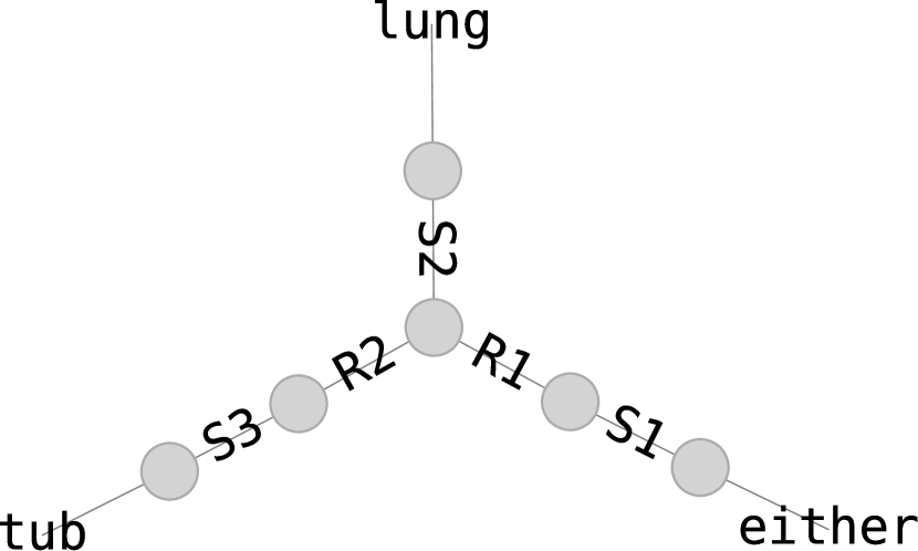
(b) TT representation of $\Phi$, without any uncertainties.

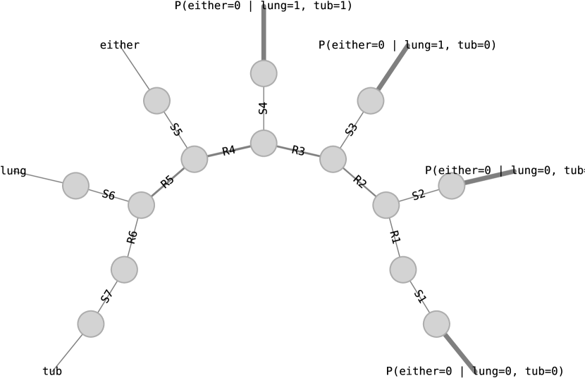
(c) TT representation of $\Phi$ after regarding four of its entries as uncertain and encoding them as additional dimensions (edges in bold).

Figure 5: Encoding four uncertainties into a 3D CPT results in a new potential of dimensionality $3+4=7$, which we compactly express using the TT format. The new indices $R_{k}$ and $S_{k}$ are virtual (in a probabilistic interpretation, they can be thought of as latent variables) and only serve to factorize the original tensor into smaller-dimensional tensors, thus avoiding an exponential increase in the number of parameters.

3.3 Computation of the Sobol Indices

The manipulations described above turn the original TN into a new one with different potentials and topology. We view the new TN as a convenient factorization of a high-dimensional function, namely the one mapping each possible value of the new variables (uncertain CPT entries) to the target probability of interest. We are now ready to obtain the Sobol indices for these variables. We do so by applying Ballester-Ripoll and Leonelli’s algorithm (Ballester-Ripoll and Leonelli, 2022a), which calculates the required variances by further transforming the TN, followed by performing ordinary inference operations on the result. We use variable elimination as our inference method, which makes the Sobol estimation exact, but other inference algorithms could be used instead.

See Fig. 6(a) for an illustration of the asia network after encoding 10 uncertain parameters.

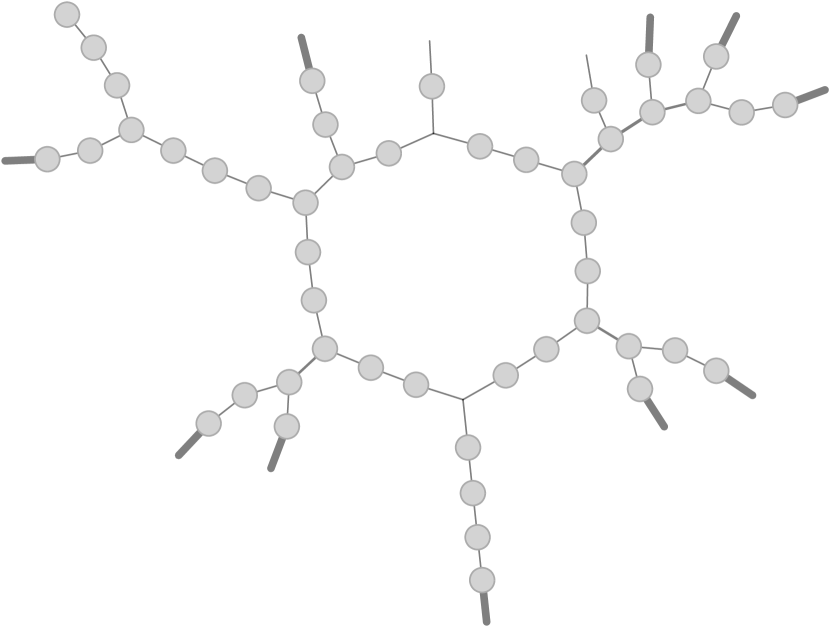
(a)

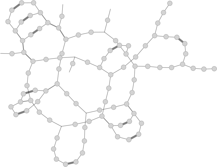
(b)

Figure 6: Left: asia network after including 10 uncertain CPT entries as new dimensions (edges in bold). Right: squared network, used to compute the network’s variance w.r.t. the 10 new dimensions in the method of Sobol Ballester-Ripoll and Leonelli (2022a), built by glueing two copies of the network along the target indices. Index names in both diagrams were omitted to avoid visual cluttering.

4 Experimental Results

4.1 Setup

Since the proposed method does not support multiple uncertainties for same-parent configurations (Sec. 3.2), we cannot consider all BN parameters as uncertain. Instead, in our experiments we use a heuristic based on the sensitivity value (Sec. 2.2) to select potentially sensitive uncertain parameters among $\bm{\theta}$:

1. Select a target probability of interest $P(Y_{O}=y_{O})$.

2. Compute the sensitivity value of all parameters of the BN using Ballester-Ripoll and Leonelli (2022b).

3. For each CPT of the BN, select the rows where all sensitivity values are non-zero.

4. For each of those rows, mark as uncertain the parameter with the highest sensitivity value.

5. Assume the the uncertain parameters are independently distributed, with each $\theta_{i}$ following a beta distribution with mean equal to its original value $\theta_{i}^{0}$ and fixed variance $\sigma^{2}$. More explicitly, $\theta_{i}\sim\text{Beta}(\alpha=\theta_{i}^{0}\lambda,\beta=(1-\theta_{i}^{0})\lambda)$ where $\lambda:=\frac{\theta_{i}^{0}-\sigma^{2}-(\theta_{i}^{0})^{2}}{\sigma^{2}}$. We will use $\sigma^{2}=0.02$ in our experiments.

Note that, instead of heuristically, the selection of uncertainties and their distributions could also be expert-elicited.

4.2 Software

Ultimately, the proposed method relies on efficient inference of large TNs to produce the desired indices. We do this via variable elimination, also known as tensor contraction in the TN literature. The order in which variables are eliminated has a massive impact on the overall computational burden, and finding the optimal order is an NP-hard problem. We use the TN contraction library cotengra (Gray and Kourtis, 2021) and its heuristic auto-hq, which offers a very good compromise between time spent on order planning and on actual evaluation. For certain tensor manipulation operations we use quimb (Gray, 2018), and we use PyTorch and YODO for calculating sensitivity values (Ballester-Ripoll and Leonelli, 2023).

4.3 Network

We next illustrate our algorithms over a BN learned from the survey “Eurobarometer 93.1: standard Eurobarometer and COVID19 Pandemic” (European Commission, 2020). Out of the many questions asked in the survey, we selected some demographic information of the respondents together with their opinion about how the COVID-19 emergency was handled by local authorities and its consequences in the long term. To avoid large number of levels and rare answers, possible categories were combined into meaningful groups. Table 1 gives details about the final 15 variables considered. Entries with missing values were dropped giving a total of 30985 observations.

Label	Question	Levels
AGE	How old are you?	18-30/30-50/51-70/70+
CLASS	Do you see yourself and your household belonging to…?	Working class/Lower class/Middle class/Upper class
COMMUNITY	Would you say you live in a…	Rural area or village/Small or middle sized town/Large town
COPING (CP)	Thinking about the measures taken to fight the Coronavirus outbreak, in particular the confinement measures, would you say that it was an experience…?	Easy to cope with/Both easy and difficult to cope with/Difficult to cope with
COUNTRYFIN (CF)	The Coronavirus outbreak will have serious economic consequences for your country	Agree/Disagree/Don’t know
GENDER	What is your sex?	Male/Female
HEALTH (HT)	Thinking about the measures taken by the public authorities in your country to fight the Coronavirus and its effects, would you say that they…	Focus too much on health/Focus too much on economivcs/Are balanced
INFO	Which of the following was your primary source of information during the Coronavirus outbreak?	Television/Written press/Radio/Websites/Social networks
JUSTIFIED (JD)	Thinking about the measures taken by the public authorities in your country to fight the Coronavirus and its effects, would you say that they were justfied?	Yes/No
LIFESAT (LS)	On the whole, are you satisfied with the life you lead?	No/Yes
OCCUPATION	Are you currently working?	Yes/No
PERSONALFIN (PF)	The Coronavirus outbreak will have serious economic consequences for you personally	Agree/Disagree/Don’t know
POLITICS	In political matters people talk of ’the left’ and ’the right’. How would you place your views on this scale?	Left/Centre/Right/Don’t know
SATMEAS (SM)	In general, are you satisfied with the measures taken to fight the Coronavirus outbreak by your government?	Yes/No
TRUST	Do you trust or not the people in your country?	Yes/No

Table 1: Details of the variables used to learn the covid-measures BN.

A BN over this dataset was learned, which we henceforth refer to as covid-measures model, with the tabu algorithm of the bnlearn R package in combination with a non-parametric bootstrap of the data (Scutari, 2010). Two-hundred replications of the data were created and for each replication a BN was learned. Edges that appeared in more than 54.5% of the learned networks were retained in the final model (this percentage was chosen using the method of Scutari and Nagarajan, 2013). The resulting network has 15 nodes, 34 edges and 588 parameters (see Fig. 7).

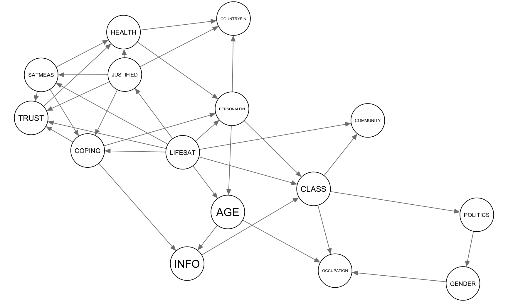
Figure 7: BN learned on the COVID-19 pandemic Eurobarometer dataset.

4.4 Analysis

We target first the probability of interest $P(\text{COUNTRYFIN}=\text{Agree})$ in the covid-measures model, and apply the proposed method to identify the most influential parameters of the BN. After restricting ourselves to the conditions detailed in Sec. 4.1, we are left with $|\bm{\theta}|=55$ uncertainties. Fig. 8 shows the resulting tensor network after baking $\bm{\theta}$ in.

Figure 8: Tensor network for the covid-measures model after encoding 55 uncertain parameters. This visualization uses the Kamada-Kawai graph layout.

The uncertainties $\bm{\theta}$ we analyzed include up to 18 entries per individual CPT, such as that of variable PERSONALFIN. After encoding, the resulting node has $3+18=21$ parents and its enriched CPT would take millions of parameters at any reasonable discretization level. However, thanks to the low-rank factorization we propose, the output tensor network from Fig. 8 only has 12’783 parameters in total, comprising tensors up to 6 dimensions and 1’026 elements only.

Fig. 9 shows the resulting top 40 BN parameters, sorted by descending total index.

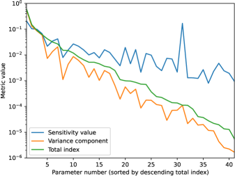
Figure 9: Sensitivity measures for the covid-measures model and target $P(\text{COUNTRYFIN}=\text{Agree})$.

There are some significant differences between the OAT analysis (the sensitivity value, in blue) and the global approach we propose. For example, the 31^st parameter has a sensitivity value of $|\partial f/\partial\theta_{31}|=0.168$ (the second highest), but its Sobol indices are almost insignificant at roughly $10^{-4}$. Conversely, the Sobol indices of the top parameter are three times larger than its sensitivity value $|\partial f/\partial\theta_{1}|=0.207$. Looking at the big picture, the Sobol indices drop much faster than the sensitivity values, suggesting that the OAT analysis overestimates the importance of most BN entries. The sensitivity values have Spearman correlations of only $0.507$ and $0.461$ with the variance components and total indices, respectively.

The proposed analysis also sheds light on the interaction between uncertain CPT entries. For each parameter $\theta_{i}$, the difference between the green and orange lines is equal to the interaction term $S_{\theta_{i}}^{T}-S_{\theta_{i}}$, which denotes how much of the parameter’s influence is due to joint effects with one or more other uncertain parameters. For example, in the case of the 9${}^{\text{th}}$ parameter in Fig. 9 , we have that $S_{\theta_{9}}^{T}$ is almost 14 times larger than $S_{\theta_{9}}$.

See Tab. 2 for the full analysis on the top 20 uncertain parameters.

CPT entry	Original value $\theta_{i}^{0}$	Sensitivity value $|\partial f/\partial\theta_{i}|$	Variance component $S_{\theta_{i}}$	$\downarrow$ Total index $S_{\theta_{i}}^{T}$
P(CP=2 |LS=1, SM=0, JD=0)	0.396000	0.001295	0.562670	0.600831
P(CF=0 |HT=0, JD=0, PF=1)	0.890525	0.103779	0.130846	0.150597
P(PF=2 |LS=0, HT=1, CP=2)	0.026115	0.009978	0.085278	0.089189
P(CP=2 |LS=0, SM=1, JD=0)	0.285907	0.002455	0.058607	0.061405
P(PF=2 |LS=1, HT=2, CP=2)	0.025797	0.006555	0.007327	0.042235
P(PF=2 |LS=0, HT=0, CP=1)	0.034884	0.009801	0.013552	0.031758
P(CF=0 |HT=2, JD=0, PF=2)	0.728324	0.011346	0.020582	0.026658
P(CF=2 |HT=0, JD=1, PF=2)	0.157303	0.002429	0.001110	0.015136
P(PF=2 |LS=1, HT=2, CP=0)	0.021277	0.003172	0.004286	0.014840
P(HT=0 |SM=1, JD=0)	0.335113	0.007694	0.008659	0.011876
P(CF=0 |HT=1, JD=1, PF=1)	0.644961	0.021831	0.006169	0.008394
P(PF=2 |LS=1, HT=0, CP=1)	0.035593	0.002300	0.003833	0.006482
P(CF=0 |HT=1, JD=0, PF=1)	0.845084	0.066525	0.001359	0.005212
P(CF=0 |HT=2, JD=1, PF=2)	0.633333	0.000948	0.002905	0.005207
P(JD=0 |LS=1, SM=1)	0.523494	0.003805	0.001030	0.004533
P(CF=0 |HT=2, JD=1, PF=0)	0.919786	0.015900	0.002478	0.003634
P(CF=1 |HT=2, JD=1, PF=1)	0.229560	0.012489	0.001911	0.003337
P(CF=0 |HT=0, JD=0, PF=2)	0.816038	0.007410	0.000662	0.002495
P(HT=0 |SM=1, JD=1)	0.530692	0.015577	0.000193	0.001103
P(CF=0 |HT=1, JD=0, PF=2)	0.712500	0.004749	0.000574	0.000991

Table 2: Top 20 measures for the covid-measures model and target $f=P(\text{COUNTRYFIN}=\text{Agree})$.

A second example with the same model, this time for target probability $P(\text{INFO}=\text{Radio})$, is shown in Fig. 10. The 8${}^{\text{th}}$ parameter, $P(\text{INFO}=\text{Radio}|\text{Age}=18-30)$, has a sensitivity value of $0.161$, apparently indicating that the effectiveness of communicating COVID-19 lockdown measures via radio channels is largely driven by the young segment. However, its Sobol indices are both below $0.0015$, revealing the parameter to be virtually irrelevant.

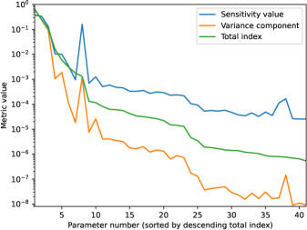
Figure 10: Sensitivity measures for the covid-measures model and target $P(\text{INFO}=\text{Radio})$. Note the blue spike denoting a large sensitivity value, whereas the Sobol indices are below 0.0015, confirming that the parameter is not relevant.

4.5 Comparison Across Networks

Last, we conduct a comparative study that applies the proposed method to the BN above as well as 7 other networks from the literature. Results are reported in Tab. 3 and include metrics about the network before and after encoding uncertain parameters, the resulting Sobol indices, and computation timings.

	alarm	crisis	child	covid- measures	hailfinder	hepar2	insurance	sachs
N. variables	$37$	$21$	$20$	$15$	$56$	$70$	$27$	$11$
Treewidth	$5$	$6$	$7$	$8$	$16$	$17$	$9$	$6$
N. parameters	$752$	$183$	$344$	$588$	$3741$	$2139$	$1419$	$267$
N. uncertainties	$7.2$	$17.6$	$25.0$	$76.2$	$8.2$	$27.6$	$32.2$	$16.2$
N. augmented parameters	$1622.2$	$974.4$	$3156.4$	$1.25\cdot 10^{5}$	$4662.2$	$4318.2$	$7480.4$	$2296.4$
Max. $S^{T}-S$	$0.022$	$0.022$	$0.02$	$0.064$	$0.084$	$0.15$	$0.018$	$0.032$
Max. $|S^{T}-f^{\prime}|$	$0.24$	$0.27$	$0.26$	$0.21$	$0.19$	$0.45$	$0.15$	$0.13$
$t_{\text{encoding}}$ (s)	$0.11$	$0.2$	$0.59$	$5.69$	$0.11$	$0.51$	$0.72$	$0.29$
$t_{\text{Sobol}}$ (s)	$0.29$	$0.38$	$0.8$	$7.67$	$0.24$	$2.58$	$1.99$	$0.44$
$t_{\text{total}}$ (s)	$0.39$	$0.58$	$1.39$	$13.36$	$0.35$	$3.1$	$2.71$	$0.74$

Table 3: Comparison across multiple BNs, including the newly learned covid-measures. Each columns was generated as the average of 5 independent runs: at each run, the target variables $Y_{O}$ and its target level $y_{o}$ were chosen at random. The network crisis is the BN proposed in Ballester-Ripoll and Leonelli (2022b); the remaining ones come from the bnlearn repository Scutari (2010).

Tab. 3 shows that interaction terms can get as large as $S^{T}-S\approx 0.15$ in the examples tested, while the difference between a total index and its corresponding sensitivity value went as high as $|S^{T}-f^{\prime}|\approx 0.45$. The table also gives insights on the typical computing times required to apply the proposed method to compute all first-order Sobol indices. It can be noticed that the encoding requires less time than computing the actual Sobol indices. In all cases the total time increases with the number of augmented parameters, which of course depend on the number of variables and the treewidth. We can see that in all cases the Sobol indices can be computed in a short amount of time, less than a second in 50% of the BNs considered.

5 Conclusions

Our work identifies the limitations of OAT-based sensitivity analysis in BNs and proposes a global, variance-based alternative that can account for multiple uncertain CPT parameters varying at once. The algorithm is based on embedding the uncertain probabilities as additional parents of the affected CPTs, and compactly encoding these augmented tables via low-rank factorization. The factorization of each CPT can be expressed as a TN, which means the resulting network is also a TN and is therefore amenable to tensor contraction (equivalent to variable elimination). Thanks to this TN formulation, we were able to apply a Sobol index computation algorithm (Ballester-Ripoll and Leonelli, 2022a) that relies on element-wise product between TNs, followed by exact tensor contraction. We demonstrate the method with a BN fitted on a real-world survey; we find cases where either the classical sensitivity value fails to account for interactions between parameters, or conversely it vastly overestimates the influence of individual parameters. The algorithm runs in a few seconds at most, even in networks with dozens of nodes and thousands of parameters. All in all, we argue the method allows analysts to conduct a broader and more informed sensitivity analysis on BNs subject to parameter uncertainty.

Despite the above, the proposed method is not free of limitations. The clearest one is its inability to model uncertainties for multiple child state probabilities given the same configuration of parents. This is because the sum-to-1 constraint introduces dependencies between those CPT entries, and the Sobol method is only suitable for non-correlated parameters of interest. However, note that this is not a problem for binary variables, since there the probabilities for alternate child states are fully linked to each other and therefore will lead to identical sensitivity indices.

Future Work

We have restricted ourselves to an exact tensor contraction scheme, as it was sufficient to compute Sobol indices from a TN that, after augmentation, comprised 50-100 nodes. For larger or topologically more complex networks, note that the TN framework opens the door to approximate contraction, which leverages SVD rank truncation to compress intermediate factors on the fly during inference. In exchange for a modest error, approximate schemes are better suited to tackle inference in challenging TNs (Gray and Chan, 2024).

As another venue of future research, upon learning which uncertain entries are the most influential in a global SA sense, one could then further obtain higher-order Sobol indices and derivations thereof in order to discern which interactions between entries are important. Options include the closed indices, the lower and upper indices, or the Shapley values (Owen, 2014), among other metrics.

References

- Ballester-Ripoll and Leonelli (2022a) Ballester-Ripoll, R., Leonelli, M., 2022a. Computing Sobol indices in probabilistic graphical models. Reliability Engineering & System Safety 225, 108573.
- Ballester-Ripoll and Leonelli (2022b) Ballester-Ripoll, R., Leonelli, M., 2022b. You only derive once (YODO): Automatic differentiation for efficient sensitivity analysis in Bayesian networks, in: International Conference on Probabilistic Graphical Models, PMLR. pp. 169–180.
- Ballester-Ripoll and Leonelli (2023) Ballester-Ripoll, R., Leonelli, M., 2023. The YODO algorithm: An efficient computational framework for sensitivity analysis in Bayesian networks. International Journal of Approximate Reasoning 159, 108929.
- Barons et al. (2022) Barons, M.J., Mascaro, S., Hanea, A.M., 2022. Balancing the elicitation burden and the richness of expert input when quantifying discrete Bayesian networks. Risk Analysis 42, 1196–1234.
- Bielza and Larrañaga (2014) Bielza, C., Larrañaga, P., 2014. Bayesian networks in neuroscience: A survey. Frontiers in Computational Neuroscience 8, 131.
- Bolt and van der Gaag (2017) Bolt, J.H., van der Gaag, L.C., 2017. Balanced sensitivity functions for tuning multi-dimensional Bayesian network classifiers. International Journal of Approximate Reasoning 80, 361–376.
- Bolt and Renooij (2014) Bolt, J.H., Renooij, S., 2014. Local sensitivity of Bayesian networks to multiple simultaneous parameter shifts, in: European Workshop on Probabilistic Graphical Models, Springer. pp. 65–80.
- Castillo et al. (1997) Castillo, E., Gutiérrez, J.M., Hadi, A.S., 1997. Sensitivity analysis in discrete Bayesian networks. IEEE Transactions on Systems, Man, and Cybernetics-Part A: Systems and Humans 27, 412–423.
- Chan and Darwiche (2004) Chan, H., Darwiche, A., 2004. Sensitivity analysis in Bayesian networks: From single to multiple parameters, in: Proocedings of the 16th Conference on Uncertainty in Artificial Intelligence, pp. 317–325.
- Chan and Darwiche (2005) Chan, H., Darwiche, A., 2005. A distance measure for bounding probabilistic belief change. International Journal of Approximate Reasoning 38, 149–174.
- Coupé et al. (2000) Coupé, V.M.H., van der Gaag, L.C., Habbema, J.D.F., 2000. Sensitivity analysis: An aid for belief-network quantification. The Knowledge Engineering Review 15, 215–232.
- Coupé and Van Der Gaag (2002) Coupé, V.M.H., Van Der Gaag, L.C., 2002. Properties of sensitivity analysis of Bayesian belief networks. Annals of Mathematics and Artificial Intelligence 36, 323–356.
- Do and Razavi (2020) Do, N.C., Razavi, S., 2020. Correlation effects? A major but often neglected component in sensitivity and uncertainty analysis. Water Resources Research 56, e2019WR025436.
- Drury et al. (2017) Drury, B., Valverde-Rebaza, J., Moura, M.F., de Andrade Lopes, A., 2017. A survey of the applications of Bayesian networks in agriculture. Engineering Applications of Artificial Intelligence 65, 29–42.
- European Commission (2020) European Commission, 2020. Eurobarometer 93.1: Eurobarometro standard e pandemia di COVID-19. Kantar Public [Producer]. GESIS - Leibniz Institute for the Social Sciences [Producer]. UniData - Bicocca Data Archive, Milano. Codice indagine SI386. Versione del file di dati 3.0.
- Giles et al. (2023) Giles, S., Errickson, D., Harrison, K., Márquez-Grant, N., 2023. Solving the inverse problem of post-mortem interval estimation using Bayesian belief networks. Forensic Science International 342, 111536.
- Gómez-Villegas et al. (2014) Gómez-Villegas, M.A., Main, P., Viviani, P., 2014. Sensitivity to evidence in Gaussian Bayesian networks using mutual information. Information Sciences 275, 115–126.
- Gray (2018) Gray, J., 2018. quimb: A Python library for quantum information and many-body calculations. Journal of Open Source Software 3, 819.
- Gray and Chan (2024) Gray, J., Chan, G.K.L., 2024. Hyperoptimized approximate contraction of tensor networks with arbitrary geometry. Physical Reviews X 14, 011009.
- Gray and Kourtis (2021) Gray, J., Kourtis, S., 2021. Hyper-optimized tensor network contraction. Quantum 5, 410.
- Hayes et al. (2012) Hayes, A.F., Glynn, C.J., Huge, M.E., 2012. Cautions regarding the interpretation of regression coefficients and hypothesis tests in linear models with interactions. Communication Methods and Measures 6, 1–11.
- Hosseini and Ivanov (2020) Hosseini, S., Ivanov, D., 2020. Bayesian networks for supply chain risk, resilience and ripple effect analysis: A literature review. Expert Systems with Applications 161, 113649.
- Jindal et al. (2022) Jindal, A., Sharma, S.K., Routroy, S., 2022. Bayesian belief network approach for supply risk modelling. International Journal of Information Systems and Supply Chain Management 15, 1–17.
- Kabir and Papadopoulos (2019) Kabir, S., Papadopoulos, Y., 2019. Applications of Bayesian networks and Petri nets in safety, reliability, and risk assessments: A review. Safety Science 115, 154–175.
- Kjærulff and van der Gaag (2000) Kjærulff, U., van der Gaag, L.C., 2000. Making sensitivity analysis computationally efficient, in: Proceedings of the 16th Conference on Uncertainty in Artificial Intelligence, pp. 317–325.
- Kolda and Bader (2009) Kolda, T.G., Bader, B.W., 2009. Tensor decompositions and applications. SIAM Review 51, 455–500.
- Koller et al. (2009) Koller, D., Friedman, N., Bach, F., 2009. Probabilistic graphical models: Principles and techniques. MIT press.
- Kwisthout and van der Gaag (2008) Kwisthout, J., van der Gaag, L., 2008. The computational complexity of sensitivity analysis and parameter tuning, in: Proceedings of the 24th Conference on Uncertainty in Artificial Intelligence, pp. 349–356.
- Laskey (1995) Laskey, K.B., 1995. Sensitivity analysis for probability assessments in Bayesian networks. IEEE Transactions on Systems, Man, and Cybernetics 25, 901–909.
- Leonelli et al. (2017) Leonelli, M., Görgen, C., Smith, J.Q., 2017. Sensitivity analysis in multilinear probabilistic models. Information Sciences 411, 84–97.
- Leonelli et al. (2023) Leonelli, M., Ramanathan, R., Wilkerson, R.L., 2023. Sensitivity and robustness analysis in Bayesian networks with the bnmonitor R package. Knowledge-Based Systems 278, 110882.
- Leonelli and Riccomagno (2022) Leonelli, M., Riccomagno, E., 2022. A geometric characterisation of sensitivity analysis in monomial models. International Journal of Approximate Reasoning 151, 64–84.
- Li and Mahadevan (2017) Li, C., Mahadevan, S., 2017. Sensitivity analysis of a Bayesian network. ASCE-ASME Journal of Risk and Uncertainty in Engineering Systems, Part J: Mechanical Engineering 4, 011003.
- Linardatos et al. (2020) Linardatos, P., Papastefanopoulos, V., Kotsiantis, S., 2020. Explainable AI: A review of machine learning interpretability methods. Entropy 23, 18.
- Ma et al. (2022) Ma, D., Zhou, T., Li, Y., Chen, J., Huang, Y., 2022. Bayesian network analysis of heat transfer deterioration in supercritical water. Nuclear Engineering and Design 391, 111733.
- Marcot and Penman (2019) Marcot, B.G., Penman, T.D., 2019. Advances in Bayesian network modelling: Integration of modelling technologies. Environmental Modelling & Software 111, 386–393.
- McLachlan et al. (2020) McLachlan, S., Dube, K., Hitman, G.A., Fenton, N., Kyrimi, E., 2020. Bayesian networks in healthcare: Distribution by medical condition. Artificial Intelligence in Medicine , 101912.
- Oseledets (2011) Oseledets, I.V., 2011. Tensor-train decomposition. SIAM Journal on Scientific Computing 33, 2295–2317.
- Owen (2014) Owen, A.B., 2014. Sobol’ indices and Shapley value. SIAM/ASA Journal on Uncertainty Quantification 2, 245–251.
- Pearl (1988) Pearl, J., 1988. Probabilistic reasoning in intelligent systems: Networks of plausible inference. Morgan Kaufmann.
- Pearl (2009) Pearl, J., 2009. Causality. Cambridge University Press.
- Razavi et al. (2021) Razavi, S., Jakeman, A., Saltelli, A., Prieur, C., Iooss, B., Borgonovo, E., Plischke, E., Lo Piano, S., Iwanaga, T., Becker, W., et al., 2021. The future of sensitivity analysis: An essential discipline for systems modeling and policy support. Environmental Modelling & Software 137, 104954.
- Renooij (2014) Renooij, S., 2014. Co-variation for sensitivity analysis in Bayesian networks: Properties, consequences and alternatives. International Journal of Approximate Reasoning 55, 1022–1042.
- Robeva and Seigal (2018) Robeva, E., Seigal, A., 2018. Duality of graphical models and tensor networks. Information and Inference: A Journal of the IMA 8, 273–288.
- Rohmer (2020) Rohmer, J., 2020. Uncertainties in conditional probability tables of discrete Bayesian belief networks: A comprehensive review. Engineering Applications of Artificial Intelligence 88, 103384.
- Rohmer and Gehl (2020) Rohmer, J., Gehl, P., 2020. Sensitivity analysis of Bayesian networks to parameters of the conditional probability model using a Beta regression approach. Expert Systems with Applications 145, 113130.
- Salmani and Katoen (2021) Salmani, B., Katoen, J.P., 2021. Fine-tuning the odds in Bayesian networks, in: European Conference on Symbolic and Quantitative Approaches with Uncertainty, Springer. pp. 268–283.
- Salmani and Katoen (2023a) Salmani, B., Katoen, J.P., 2023a. Automatically finding the right probabilities in Bayesian networks. Journal of Artificial Intelligence Research 77, 1637–1696.
- Salmani and Katoen (2023b) Salmani, B., Katoen, J.P., 2023b. Finding an -close minimal variation of parameters in Bayesian networks, in: Proceedings of the Thirty-Second International Joint Conference on Artificial Intelligence, pp. 5720–5729.
- Saltelli et al. (2019) Saltelli, A., Aleksankina, K., Becker, W., Fennell, P., Ferretti, F., Holst, N., Li, S., Wu, Q., 2019. Why so many published sensitivity analyses are false: A systematic review of sensitivity analysis practices. Environmental Modelling & Software 114, 29–39.
- Saltelli et al. (2021) Saltelli, A., Jakeman, A., Razavi, S., Wu, Q., 2021. Sensitivity analysis: A discipline coming of age. Environmental Modelling & Software 146, 105226.
- Saltelli et al. (2008) Saltelli, A., Ratto, M., Andres, T., Campolongo, F., Cariboni, J., Gatelli, D., Saisana, M., Tarantola, S., 2008. Global Sensitivity Analysis: The Primer. John Wiley & Sons, Ltd.
- Saltelli et al. (2000) Saltelli, A., Tarantola, S., Campolongo, F., 2000. Sensitivity analysis as an ingredient of modeling. Statistical Science 15, 377–395.
- Schneider and Uschmajew (2014) Schneider, R., Uschmajew, A., 2014. Approximation rates for the hierarchical tensor format in periodic Sobolev spaces. Journal of Complexity 30, 56–71. Dagstuhl 2012.
- Scutari (2010) Scutari, M., 2010. Learning Bayesian networks with the bnlearn R package. Journal of Statistical Software 35, 1–22.
- Scutari et al. (2019) Scutari, M., Graafland, C.E., Gutiérrez, J.M., 2019. Who learns better Bayesian network structures: Accuracy and speed of structure learning algorithms. International Journal of Approximate Reasoning 115, 235–253.
- Scutari and Nagarajan (2013) Scutari, M., Nagarajan, R., 2013. Identifying significant edges in graphical models of molecular networks. Artificial Intelligence in Medicine 57, 207–217.
- Sobol (1990) Sobol, I.M., 1990. Sensitivity estimates for nonlinear mathematical models (in Russian). Mathematical Models 2, 112–118.
- Van Der Gaag et al. (2007) Van Der Gaag, L.C., Renooij, S., Coupé, V.M., 2007. Sensitivity analysis of probabilistic networks, in: Advances in Probabilistic Graphical Models. Springer, pp. 103–124.
- Van Stein et al. (2022) Van Stein, B., Raponi, E., Sadeghi, Z., Bouman, N., Van Ham, R.C., Bäck, T., 2022. A comparison of global sensitivity analysis methods for explainable AI with an application in genomic prediction. IEEE Access 10, 103364–103381.
- Wang et al. (2023) Wang, J., Zhai, X., Luo, Q., 2023. Chinese travellers’ mobility decision-making processes during public health crisis situations: A Bayesian network model. Current Issues in Tourism 26, 1828–1844.
- Zio et al. (2022) Zio, E., Mustafayeva, M., Montanaro, A., 2022. A Bayesian belief network model for the risk assessment and management of premature screen-out during hydraulic fracturing. Reliability Engineering & System Safety 218, 108094.