The quantum-refractive evolution of polarization states in pulsar emission

Abstract

Highly magnetized neutron stars have quantum refraction effects on pulsar emission due to the non-linearity of the quantum electrodynamics (QED) action. In this paper, we investigate the evolution of the polarization states under the quantum refraction effects combined with the frequency dependence of pulsar emission; we solve a system of evolution equations of the Stokes vector, where the birefringent vector, in which such effects are encoded, acts on the Stokes vector. At a fixed frequency of emission, depending on the magnitude of the birefringent vector, dominated mostly by the magnetic field strength, the evolution of the Stokes vector largely exhibits three different patterns: (i) monotonic, or (ii) half-oscillatory, or (iii) highly oscillatory behaviours. These features are understood and confirmed by means of approximate analytical solutions to the evolution equations.

1 Introduction

Highly magnetized neutron stars are interesting astrophysical objects that will provide an astrophysical arena for probing fundamental physics (Raffelt (1996)), in particular, strong field QED (Meszaros (1992); Harding & Lai (2006)). The magnetic fields of neutron stars of $10^{12}-10^{15}\,\mathrm{G}$ are strong enough to give rise to QED effects, such as vacuum polarization and pair production due to the induced electric fields, which have been proposed as an astrophysical laboratory to test strong field QED (see Kim & Kim (2021) and references therein). A great advantage of neutron stars as a laboratory is virtually infinitely long duration and range of the electromagnetic fields (in the scale of Compton time and length), strongly contrasting with the short, pulsed fields achieved with ultra-intense lasers, as well as the strength of the fields (Yoon et al. (2021)).

Strong electromagnetic fields polarize the vacuum, which leads to the Heisenberg-Euler-Schwinger (HES) one-loop effective action (Heisenberg & Euler (1936); Schwinger (1951)). The effective action describes non-linear electrodynamics, which has an imaginary part from the vacuum instability due to production of charged particle pairs via electric fields. The HES action leads to the vacuum multiple refraction indices, which is generally referred to as the quantum refraction effect. A test of strong-field QED is one of the most important problems in physics, and there have been laboratory experiment proposals for it, e.g., PVLAS (Polarizzazione del Vuoto con LAser) project (Ejlli et al. (2020)). On the other hand, highly magnetized neutron stars provide near-critical fields, and these can be used as various celestial laboratories to test strong field QED (Ruffini et al. (2010); Fedotov et al. (2023); Hattori et al. (2023))). Also, there have been space missions proposed to observe the strong-field QED effects, e.g., the enhanced X-ray Timing and Polarimetry (eXTP) (Santangelo et al. (2019)) and the Compton Telescope project (Wadiasingh et al. (2019)).

The HES action is well approximated by the post-Maxwellian action, even up to the strength one order lower than the critical magnetic field $B_{\mathrm{c}}=m_{\mathrm{e}}^{2}c^{3}/e\hbar=4.4\times 10^{13}\,\mathrm{G}$, which keeps up to the quadratic terms of the Maxwell scalar and pseudo-scalar. Therefore, the post-Maxwellian action exhibits non-linear characteristics of vacuum polarization, such as quantum refraction. Previously, we have studied the quantum refraction effects on the polarization vectors in the dipole magnetic field background of a pulsar model (Kim et al. (2024)). The study is non-trivial in comparison with other similar studies where the background magnetic field is assumed to be uniform, in that we have to deal with dipole magnetic field, whose strength and direction vary over space.

In this paper, we study the evolution of the polarization states under the quantum refraction effects combined with the frequency dependence of pulsar emission. Our analysis is based on the evolution equations of the Stokes vector, where such effects are encoded into the birefringent vector that acts on the Stokes vector. The Stokes vector has a crucial advantage over the polarization vector in representing polarization states: it can be directly determined from experimentally measurable quantities and accommodate depolarization effects due to incomplete coherence and random processes during the photon propagation. Solutions of the evolution equations describe how the polarization states change along the photon propagation path from the emission point towards an observer. It turns out that the evolution of the Stokes vector, at a fixed frequency of emission, largely exhibits three different patterns, depending on the magnitudes of the birefringent vector, dominated mostly by the magnetic field strength: (i) fractionally oscillatory - monotonic, or (ii) half-oscillatory, or (iii) highly oscillatory behaviours, which are found by numerical solutions and also confirmed by approximate analytical solutions. These are novel features rarely illuminated in previous studies on the same topic.

The paper is organized as follows. In Section 2.1, we introduce a system of evolution equations of the Stokes vector and apply this formalism to our pulsar emission model for an oblique rotator. In Section 2.2, the evolution equations are solved for some known rotation-powered pulsars (RPPs) in three ways: fully numerically, via perturbation analysis, and using an analytical approximation. Also, we discuss the evolution patterns of the Stokes vectors resulting from the solutions. Then finally, we conclude the paper with discussions on other similar studies and follow-up studies.

2 Evolution of Stokes vector in strong magnetic field

2.1 Evolution equations of Stokes vector

Classically, polarization properties of pulsar emission are described by the Stokes parameters $\left\{I,Q,U,V\right\}$, where $I$ is a measure of the total intensity, $Q$ and $U$ jointly describe the linear polarization, and $V$ describes the circular polarization of the curvature emission in pulsars (for more details, see Appendix A). However, in the presence of strong magnetic fields in the background of the emission, the polarization evolves along the photon propagation path from the emission point towards an observer. The evolution of the polarization can be investigated systematically using the formalism initiated by Kubo & Nagata (1981, 1983, 1985), and further developed by Heyl & Shaviv (2000), Heyl et al. (2003), Heyl & Caiazzo (2018), and Novak et al. (2018), namely, a system of evolution equations of the Stokes vector, described as

$$\frac{\mathrm{d}\mathbf{S}}{\mathrm{d}s}=k\mathbf{\hat{\Omega}}\times\mathbf{S},$$ (1)

where $k\equiv\omega/c$ denotes the wave number for the electromagnetic radiation and $s$ is an affine parameter to measure the length of the photon trajectory, and $\mathbf{S}$ is the normalized Stokes vector, defined out of the Stokes parameters as $\mathbf{S}=\left(S_{1},S_{2},S_{3}\right)\allowbreak\equiv\left(Q/I,U/I,V/I\right)$, and $\mathbf{\hat{\Omega}}$ is the birefringent vector, defined as

$$\mathbf{\hat{\Omega}}\equiv\frac{\alpha_{\mathrm{e}}}{30\pi}\left(B/B_{\mathrm{c}}\right)^{2}\sin^{2}\vartheta\left(\mathcal{E}_{\mathrm{I}}^{2}-\mathcal{E}_{\mathrm{II}}^{2},2\mathcal{E}_{\mathrm{I}}\mathcal{E}_{\mathrm{II}},0\right),$$ (2)

where $\alpha_{\mathrm{e}}$ denotes the fine-structure constant and $\alpha_{\mathrm{e}}/\left(30\pi\right)\approx 7.743\times 10^{-5}$ and $B_{\mathrm{c}}\approx 4.414\times 10^{13}\,\mathrm{G}$ is the critical magnetic field, and $\vartheta$ denotes the angle between the photon trajectory and the local magnetic field line (see Fig. 1), i.e.,

$$\vartheta=\cos^{-1}\left(\mathbf{\hat{n}}_{\left[0\right]}\cdot\mathbf{\hat{B}}\right),$$ (3)

with $\mathbf{\hat{n}}_{\left[0\right]}$ being the classical propagation vector and $\mathbf{\hat{B}}\equiv\mathbf{B}/\left|\mathbf{B}\right|$, and

$$\mathcal{E}_{i}\equiv-\mathbf{\hat{B}\cdot}\left(\mathbf{\hat{n}}_{\left[0\right]}\times\boldsymbol{\varepsilon}_{i\left[0\right]}\right),~{}~{}i=\mathrm{I},\mathrm{II},$$ (4)

with $\boldsymbol{\varepsilon}_{\mathrm{I}\left[0\right]}$ and $\boldsymbol{\varepsilon}_{\mathrm{II}\left[0\right]}$ being the two classical mode polarization vectors, orthogonal to each other and to $\mathbf{\hat{n}}_{\left[0\right]}$; the specific forms of $\mathbf{\hat{n}}_{\left[0\right]}$, $\boldsymbol{\varepsilon}_{\mathrm{I}\left[0\right]}$ and $\boldsymbol{\varepsilon}_{\mathrm{II}\left[0\right]}$ are later given by equations (8), (12) and (13), respectively, for the magnetic field of an oblique dipole rotator as described by equation (5) and Fig. 1.

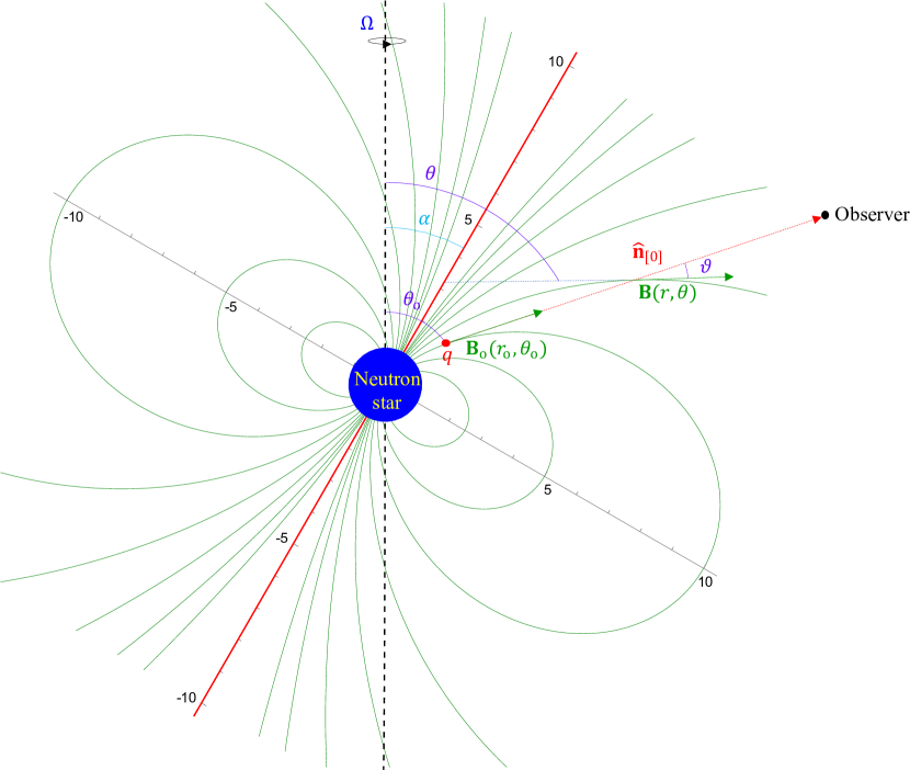
Figure 1: A cross-sectional view of a pulsar magnetosphere with the dipole magnetic field lines (green) around a neutron star. The vertical dashed line (black) and the inclined solid line (red) represent the rotation axis and the magnetic axis, respectively. $\alpha$ between these axes denotes the inclination angle. The scale of the unity in this graph is equivalent to the neutron star radius $\sim 10^{6}\,\mathrm{cm}$. The red dotted line represents the trajectory curve of the light ray traced by $\mathbf{\hat{n}}_{\left[0\right]}$ as projected onto the $xz$-plane. (Credit: Kim & Trippe (2021), reproduced with modifications.)

In our pulsar emission model, we consider curvature radiation produced along the magnetic field lines of an oblique dipole rotator as illustrated in Fig. 1:

$$\mathbf{B}\left(r,\theta,\phi\right)=\frac{2\mu\left(\cos\alpha\cos\theta+\sin\alpha\sin\theta\cos\phi\right)}{r^{3}}\mathbf{e}_{\hat{r}}+\frac{\mu\left(\cos\alpha\sin\theta-\sin\alpha\cos\theta\cos\phi\right)}{r^{3}}\mathbf{e}_{\hat{\theta}}+\frac{\mu\sin\alpha\sin\phi\,}{r^{3}}\mathbf{e}_{\hat{\phi}},$$ (5)

where $\mu$ is the magnetic dipole moment and $\alpha$ denotes the inclination angle between the rotation axis and the magnetic axis. The photon beam from curvature radiation is tangent to the field line at the emission point $\left(x_{\mathrm{o}},y_{\mathrm{o}},z_{\mathrm{o}}\right)=\left(r_{\mathrm{o}}\sin\theta_{\mathrm{o}},0,r_{\mathrm{o}}\cos\theta_{\mathrm{o}}\right)$.

However, at the same time, our pulsar magnetosphere rotates, and therefore the field lines get twisted due to the magneto-centrifugal acceleration on the plasma particles moving along the field lines (Blandford & Payne (1982)). Then, taking into consideration this magneto-hydrodynamic (MHD) effect, the direction of the classical photon propagation, which must line up with the particle velocity in order for an observer to receive the radiation, can be described as (Gangadhara (2005))

$$\mathbf{\hat{n}}_{\left[0\right]}=\beta\mathbf{\hat{B}}+\mathbf{\Omega}_{\mathrm{p}}\times\mathbf{r,}$$ (6)

where on the right-hand side

$$\beta\equiv\left[1-\left(\frac{\Omega_{\mathrm{p}}r}{c}\right)^{2}\sin^{2}\theta\left(1-\frac{\sin^{2}\alpha\sin^{2}\phi}{3\cos^{2}\theta^{\prime}+1}\right)\right]^{1/2}-\frac{\Omega_{\mathrm{p}}r}{c}\frac{\sin\alpha\sin\theta\sin\phi}{\left(3\cos^{2}\theta^{\prime}+1\right)^{1/2}},$$ (7)

with $c$ being the speed of light and $\cos\theta^{\prime}\equiv\cos\alpha\cos\theta+\sin\alpha\sin\theta\cos\phi$, and the second term accounts for the centrifugal acceleration, with $\mathbf{\Omega}_{\mathrm{p}}\equiv\Omega_{\mathrm{p}}\mathbf{e}_{z}$ and $\Omega_{\mathrm{p}}=2\pi/P$ being a pulsar rotation (angular) frequency, as given in terms of the rotation period $P$.

During the rotation the azimuthal phase changes by $\phi\sim\Omega_{\mathrm{p}}t$, while our photon has propagated a distance by $s\sim ct$. In our analysis, the photon propagation is described with the consideration of the MHD effect above, assuming $\phi$ to be very small; e.g., $\phi\lesssim 10^{-1}$ is considered for a millisecond pulsar with $\Omega_{\mathrm{p}}\sim 10^{2}\,\mathrm{Hz}$, during the time of rotation $t\lesssim 10^{-3}\,\mathrm{s}$, such that $s\lesssim 10^{7}\,\mathrm{cm}$, which corresponds to the propagation distance within about $10$ times the neutron star radius. For equation (6) we take only the leading order expansions of $\mathbf{\hat{B}}\left(r_{\mathrm{o}},\theta_{\mathrm{o}},\phi\right)$ and $\beta\left(r_{\mathrm{o}},\theta_{\mathrm{o}},\phi\right)$ in $\phi$ from equations (5) and (7), respectively, and can express the classical propagation vector $\mathbf{\hat{n}}_{\left[0\right]}$ in Cartesian coordinates as

$$\mathbf{\hat{n}}_{\left[0\right]}=\hat{n}_{x\left[0\right]}\mathbf{e}_{x}+\hat{n}_{y\left[0\right]}\mathbf{e}_{y}+\hat{n}_{z\left[0\right]}\mathbf{e}_{z}\\$$ (8)

with

$$\hat{n}_{x\left[0\right]} \approx\frac{2\cos\left(\theta_{\mathrm{o}}-\alpha\right)\sin\theta_{\mathrm{o}}+\sin\left(\theta_{\mathrm{o}}-\alpha\right)\cos\theta_{\mathrm{o}}}{\left(3\cos^{2}\left(\theta_{\mathrm{o}}-\alpha\right)+1\right)^{1/2}}+\mathcal{O}\left(\phi^{2},\left(\Omega_{\mathrm{p}}r_{\mathrm{o}}/c\right)^{2},\phi\left(\Omega_{\mathrm{p}}r_{\mathrm{o}}/c\right)\right),$$ (9)

$$\hat{n}_{z\left[0\right]} \approx\frac{2\cos\left(\theta_{\mathrm{o}}-\alpha\right)\cos\theta_{\mathrm{o}}-\sin\left(\theta_{\mathrm{o}}-\alpha\right)\sin\theta_{\mathrm{o}}}{\left(3\cos^{2}\left(\theta_{\mathrm{o}}-\alpha\right)+1\right)^{1/2}}+\mathcal{O}\left(\phi^{2},\left(\Omega_{\mathrm{p}}r_{\mathrm{o}}/c\right)^{2},\phi\left(\Omega_{\mathrm{p}}r_{\mathrm{o}}/c\right)\right),$$ (10)

and

$$\hat{n}_{y\left[0\right]}\approx\frac{\Omega_{\mathrm{p}}}{c}\left[\frac{\sin\alpha s}{\left(3\cos^{2}\left(\theta_{\mathrm{o}}-\alpha\right)+1\right)^{1/2}}+r_{\mathrm{o}}\sin\theta_{\mathrm{o}}\right]+\mathcal{O}\left(\phi^{2},\left(\Omega_{\mathrm{p}}r_{\mathrm{o}}/c\right)^{2},\phi\left(\Omega_{\mathrm{p}}r_{\mathrm{o}}/c\right)\right),$$ (11)

where we have considered $\Omega_{\mathrm{p}}r_{\mathrm{o}}/c\lesssim\phi$, e.g., for a millisecond pulsar with $\Omega_{\mathrm{p}}\sim 10^{2}\,\mathrm{Hz}$ and $r_{\mathrm{o}}\sim 10^{6}\,\mathrm{cm}$, such that $\left(\Omega_{\mathrm{p}}r_{\mathrm{o}}/c\right)^{2}\lesssim\phi\left(\Omega_{\mathrm{p}}r_{\mathrm{o}}/c\right)\lesssim\phi^{2}$, all to be ignored in our analysis, and have substituted $\phi=\Omega_{\mathrm{p}}s/c$ in equation (11), the leading order rotational effect to be considered in our analysis.

The orthogonal pair of classical mode polarization vectors, $\boldsymbol{\varepsilon}_{\mathrm{I}\left[0\right]}$ and $\boldsymbol{\varepsilon}_{\mathrm{II}\left[0\right]}$, both being also orthogonal to $\mathbf{\hat{n}}_{\left[0\right]}$ as given by equation (8) above, are determined as

$$\boldsymbol{\varepsilon}_{\mathrm{I}\left[0\right]} =\hat{n}_{z\left[0\right]}\mathbf{e}_{x}+\hat{n}_{y\left[0\right]}\mathbf{e}_{y}-\hat{n}_{x\left[0\right]}\mathbf{e}_{z},$$ (12)

$$\boldsymbol{\varepsilon}_{\mathrm{II}\left[0\right]} =-\left(\hat{n}_{x\left[0\right]}+\hat{n}_{z\left[0\right]}\right)\hat{n}_{y\left[0\right]}\mathbf{e}_{x}+\mathbf{e}_{y}+\left(\hat{n}_{x\left[0\right]}-\hat{n}_{z\left[0\right]}\right)\hat{n}_{y\left[0\right]}\mathbf{e}_{z},$$ (13)

such that the three vectors, $\mathbf{\hat{n}}_{\left[0\right]}$, $\boldsymbol{\varepsilon}_{\mathrm{I}\left[0\right]}$ and $\boldsymbol{\varepsilon}_{\mathrm{II}\left[0\right]}$ form an orthonormal basis. Using these for equation (4), we obtain

$$\mathcal{E}_{\mathrm{I}} =-\mathbf{\hat{B}\cdot}\left(\mathbf{\hat{n}}_{\left[0\right]}\times\boldsymbol{\varepsilon}_{\mathrm{I}\left[0\right]}\right)$$

$$\approx\frac{4\cos\left(\theta_{\mathrm{o}}-\alpha\right)\cos\left(\theta-\alpha\right)+\sin\left(\theta_{\mathrm{o}}-\alpha\right)\sin\left(\theta-\alpha\right)+2\sin\left(\theta-\theta_{\mathrm{o}}\right)}{\left(3\cos^{2}\left(\theta_{\mathrm{o}}-\alpha\right)+1\right)^{1/2}\left(3\cos^{2}\left(\theta-\alpha\right)+1\right)^{1/2}}\hat{n}_{y\left[0\right]}-\frac{\Omega_{\mathrm{p}}\sin\alpha s}{c\left(3\cos^{2}\left(\theta-\alpha\right)+1\right)^{1/2}}$$

$$\hskip 10.0pt+\mathcal{O}\left(\phi^{2},\left(\Omega_{\mathrm{p}}r_{\mathrm{o}}/c\right)^{2},\phi\left(\Omega_{\mathrm{p}}r_{\mathrm{o}}/c\right)\right),$$ (14)

$$\mathcal{E}_{\mathrm{II}} =-\mathbf{\hat{B}\cdot}\left(\mathbf{\hat{n}}_{\left[0\right]}\times\boldsymbol{\varepsilon}_{\mathrm{II}\left[0\right]}\right)$$

$$\approx-\frac{2\sin\left(\theta-\theta_{\mathrm{o}}\right)}{\left(3\cos^{2}\left(\theta_{\mathrm{o}}-\alpha\right)+1\right)^{1/2}\left(3\cos^{2}\left(\theta-\alpha\right)+1\right)^{1/2}}+\mathcal{O}\left(\phi^{2},\left(\Omega_{\mathrm{p}}r_{\mathrm{o}}/c\right)^{2},\phi\left(\Omega_{\mathrm{p}}r_{\mathrm{o}}/c\right)\right).$$ (15)

By means of equations (3), (5) and (8) one can express

$$\cos\vartheta \approx\frac{4\cos\left(\theta_{\mathrm{o}}-\alpha\right)\cos\left(\theta-\alpha\right)+\sin\left(\theta_{\mathrm{o}}-\alpha\right)\sin\left(\theta-\alpha\right)}{\left(3\cos^{2}\left(\theta_{\mathrm{o}}-\alpha\right)+1\right)^{1/2}\left(3\cos^{2}\left(\theta-\alpha\right)+1\right)^{1/2}}+\mathcal{O}\left(\phi^{2},\left(\Omega_{\mathrm{p}}r_{\mathrm{o}}/c\right)^{2},\phi\left(\Omega_{\mathrm{p}}r_{\mathrm{o}}/c\right)\right),$$ (16)

$$\sin\vartheta \approx\frac{2\sin\left(\theta-\theta_{\mathrm{o}}\right)}{\left(3\cos^{2}\left(\theta_{\mathrm{o}}-\alpha\right)+1\right)^{1/2}\left(3\cos^{2}\left(\theta-\alpha\right)+1\right)^{1/2}}+\mathcal{O}\left(\phi^{2},\left(\Omega_{\mathrm{p}}r_{\mathrm{o}}/c\right)^{2},\phi\left(\Omega_{\mathrm{p}}r_{\mathrm{o}}/c\right)\right).$$ (17)

Now, using the relations between equations (14), (15) and (16), (17), the birefringent vector can finally be specified from equation (2):

$$\hat{\Omega}_{1} \approx-\eta B^{2}\sin^{4}\vartheta+\mathcal{O}\left(\phi^{2},\left(\Omega_{\mathrm{p}}r_{\mathrm{o}}/c\right)^{2},\phi\left(\Omega_{\mathrm{p}}r_{\mathrm{o}}/c\right)\right),$$ (18)

$$\hat{\Omega}_{2} \approx 2\eta B^{2}\sin^{3}\vartheta\left[\left(\cos\vartheta+\sin\vartheta\right)\hat{n}_{y\left[0\right]}-\frac{\Omega_{\mathrm{p}}\sin\alpha s}{c\left(3\cos^{2}\left(\theta-\alpha\right)+1\right)^{1/2}}\right]+\mathcal{O}\left(\phi^{2},\left(\Omega_{\mathrm{p}}r_{\mathrm{o}}/c\right)^{2},\phi\left(\Omega_{\mathrm{p}}r_{\mathrm{o}}/c\right)\right),$$ (19)

where $\eta\equiv\alpha_{\mathrm{e}}/\left(30\pi B_{\mathrm{c}}^{2}\right)$ and

$$B=\frac{B_{\mathrm{max}}r_{*}^{3}\ \left(3\cos^{2}\left(\theta-\alpha\right)+1\right)^{1/2}}{2\left(x^{2}+z^{2}\right)^{3/2}},$$ (20)

with $B_{\mathrm{max}}$ being the maximum magnetic field strength at the polar cap and $r_{*}$ being the neutron star radius ($\approx 10^{6}\,\mathrm{cm}$), and $\hat{n}_{y\left[0\right]}$, $\cos\vartheta$ and $\sin\vartheta$ are given by equations (11), (16) and (17), respectively.

To facilitate solving the evolution equations (1) in the next Subsection, we substitute the following identities,

$$\cos\left(\theta-\alpha\right)=\frac{\sin\alpha x+\cos\alpha z}{\left(x^{2}+z^{2}\right)^{1/2}},~{}~{}\sin\left(\theta-\alpha\right)=\frac{\cos\alpha x-\sin\alpha z}{\left(x^{2}+z^{2}\right)^{1/2}},~{}~{}\sin\left(\theta-\theta_{\mathrm{o}}\right)=\frac{\cos\theta_{\mathrm{o}}x-\sin\theta_{\mathrm{o}}z}{\left(x^{2}+z^{2}\right)^{1/2}},$$ (21)

together with

$$x=\hat{n}_{x\left[0\right]}s+r_{\mathrm{o}}\sin\theta_{\mathrm{o}},~{}~{}z=\hat{n}_{z\left[0\right]}s+r_{\mathrm{o}}\cos\theta_{\mathrm{o}}$$ (22)

into (16) and (17). Then our solutions for the Stokes vector $\mathbf{S}$ will be parametrised by $s$.

2.2 Solving evolution equations

From equation (1) we write down a system of first-order ordinary differential equations to solve:

$$\dot{S}_{1}\left(s\right) =k\hat{\Omega}_{2}\left(s\right)S_{3}\left(s\right),$$ (23)

$$\dot{S}_{2}\left(s\right) =-k\hat{\Omega}_{1}\left(s\right)S_{3}\left(s\right),$$ (24)

$$\dot{S}_{3}\left(s\right) =k\left[\hat{\Omega}_{1}\left(s\right)S_{2}\left(s\right)-\hat{\Omega}_{2}\left(s\right)S_{1}\left(s\right)\right],$$ (25)

where an over-dot ${\dot{}}$ denotes differentiation with respect to $s$, and $\hat{\Omega}_{1}\left(s\right)$ and $\hat{\Omega}_{2}\left(s\right)$ are given by (18) and (19), respectively. By solving these equations numerically, we find out how the photon polarization evolves through the strong magnetic field in the background of our pulsar emission.

However, in case $\left|k\hat{\Omega}_{1,2}\left(s\right)s\right|_{\mathrm{max}}\ll 1$, one can obtain a solution to equation (1) via perturbation:

$$\mathbf{S}=\mathbf{S}_{\left[0\right]}+\delta\mathbf{S}_{\left[1\right]}=\mathbf{S}_{\left[0\right]}+k\int\mathbf{\hat{\Omega}}\times\mathbf{S}_{\left[0\right]}\,\mathrm{d}s,$$ (26)

where $\delta\mathbf{S}_{\left[1\right]}$ means the leading order quantum correction to the unperturbed (initial) Stokes vector $\mathbf{S}_{\left[0\right]}$. Here the correction can be treated as the leading order perturbation with $\alpha_{\mathrm{e}}/\left(30\pi\right)\left(B/B_{\mathrm{c}}\right)^{2}\sim 10^{-5}\left(B/B_{\mathrm{c}}\right)^{2}$ being a perturbation parameter. Upon inspection of equations (18) and (19) for equation (26), we can further write down our solution in terms of its components:

$$S_{1} \approx S_{1\left[0\right]}+2k\eta S_{3\left[0\right]}\int B^{2}\sin^{3}\vartheta\left[\left(\cos\vartheta+\sin\vartheta\right)\hat{n}_{y\left[0\right]}-\frac{\Omega_{\mathrm{p}}\sin\alpha s}{c\left(3\cos^{2}\left(\theta-\alpha\right)+1\right)^{1/2}}\right]\mathrm{d}s,$$ (27)

$$S_{2} \approx S_{2\left[0\right]}+k\eta S_{3\left[0\right]}\int B^{2}\sin^{4}\vartheta\mathrm{d}s,$$ (28)

$$S_{3} \approx S_{3\left[0\right]}-k\eta\left\{S_{2\left[0\right]}\int B^{2}\sin^{4}\vartheta\mathrm{d}s+2S_{1\left[0\right]}\int B^{2}\sin^{3}\vartheta\left[\left(\cos\vartheta+\sin\vartheta\right)\hat{n}_{y\left[0\right]}-\frac{\Omega_{\mathrm{p}}\sin\alpha s}{c\left(3\cos^{2}\left(\theta-\alpha\right)+1\right)^{1/2}}\right]\mathrm{d}s\right\}.$$ (29)

2.2.1 Examples

We consider X-ray emissions from three neutron stars, (i) one with $B_{\mathrm{max}}\approx 10^{12}\,\mathrm{G}$ and $\Omega_{\mathrm{p}}\approx 392.7\,\mathrm{Hz}$ ($P\approx 0.016\,\mathrm{s}$), (ii) another with $B_{\mathrm{max}}\approx 5.6\times 10^{12}\,\mathrm{G}$ and $\Omega_{\mathrm{p}}\approx 22.28\,\mathrm{Hz}$ ($P\approx 0.282\,\mathrm{s}$), (iii) the third with $B_{\mathrm{max}}\approx 5.0\times 10^{13}\,\mathrm{G}$ and $\Omega_{\mathrm{p}}\approx 19.6\,\mathrm{Hz}$ ($P\approx 0.32\,\mathrm{s}$), and assume for all the emissions, $r_{\mathrm{o}}=2r_{*}\approx 2\times 10^{6}\,\mathrm{cm}$, $\theta_{\mathrm{o}}=60^{\circ}$, $\alpha=45^{\circ}$, $\eta\approx 3.97\times 10^{-32}$ and $\omega\approx 2\pi\times 10^{18}\,\mathrm{Hz}$ ($k\approx 2.0958\times 10^{8}\,\mathrm{cm^{-1}}$). These stars belong to ‘rotation-powered pulsars’ (RPPs) (Pavlov et al. (2013)). In Fig. 2 the three RPPs chosen from the X-ray group are encircled, (i) the one in orange, (ii) another in cyan, (iii) the third in green. Given the X-ray emissions from these, we solve the evolution equations (1) for the following cases.

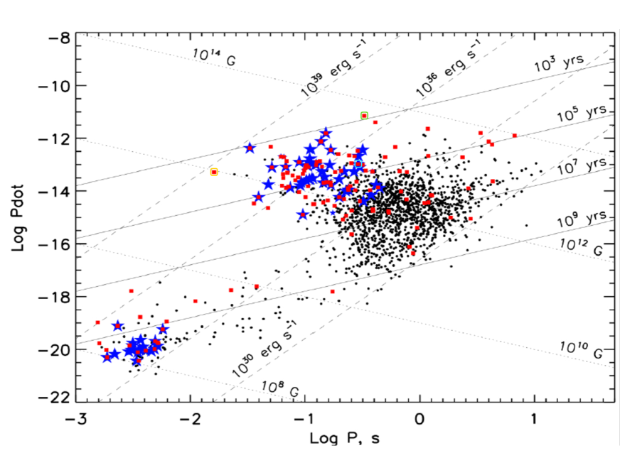
Figure 2: The population of detected rotation-powered pulsars (RPPs) plotted against their rotation period. RPPs detected in X-rays and gamma-rays are represented by red dots and blue stars, respectively. Three RPPs chosen from the X-ray group, (i) one with $B_{\mathrm{max}}\approx 10^{12}\,\mathrm{G}$ and $\Omega_{\mathrm{p}}\approx 392.7\,\mathrm{Hz}$ ($P\approx 0.016\,\mathrm{s}$), (ii) another with $B_{\mathrm{max}}\approx 5.6\times 10^{12}\,\mathrm{G}$ and $\Omega_{\mathrm{p}}\approx 22.28\,\mathrm{Hz}$ ($P\approx 0.282\,\mathrm{s}$), (iii) the third with $B_{\mathrm{max}}\approx 5.0\times 10^{13}\,\mathrm{G}$ and $\Omega_{\mathrm{p}}\approx 19.6\,\mathrm{Hz}$ ($P\approx 0.32\,\mathrm{s}$), are encircled in orange, cyan and green colours, respectively. (Credit: Pavlov et al. (2013), reproduced with modifications.)

Example (i)

With $B_{\mathrm{max}}\approx 10^{12}\,\mathrm{G}$ and $\Omega_{\mathrm{p}}\approx 392.7\,\mathrm{Hz}$ ($P\approx 0.016\,\mathrm{s}$), we obtain numerical solutions through equations (23)-(25) (in solid lines) or perturbative solutions by means of equations (27)-(29) (in dashed lines), as shown in Figs. 3a and 3b, given the initial Stokes vectors $\mathbf{S}\left(0\right)=\left(S_{1}\left(0\right),S_{2}\left(0\right),S_{3}\left(0\right)\right)=\left(1,0,0\right)$ and $\left(0.8,0,0.6\right)$, respectively. The perturbative solutions agree well with numerical ones as $\left|k\hat{\Omega}_{1,2}\left(s\right)s\right|_{\mathrm{max}}\sim\left|k\hat{\Omega}_{1,2\left(\mathrm{min}\right)}s_{\dagger 1,2}\right|\sim 10^{-2}\ll 1$, where $\hat{\Omega}_{1,2\left(\mathrm{min}\right)}\equiv\hat{\Omega}_{1,2}\left(s_{\dagger 1,2}\right)$, evaluated from the birefringent functions given by (18), (19), with $s_{\dagger 1,2}$ being the extremum, i.e., $\mathrm{d}\hat{\Omega}_{1,2}\left(s_{\dagger 1,2}\right)/\mathrm{d}s=0$. On the Poincaré sphere, our solutions are represented by the magenta and light blue loci in Fig. 6a, corresponding to Figs. 3a and 3b, respectively. The loci imply a fraction of an oscillation for the polarization evolution, as is confirmed later by the approximate analytical solutions in Section 2.2.2.

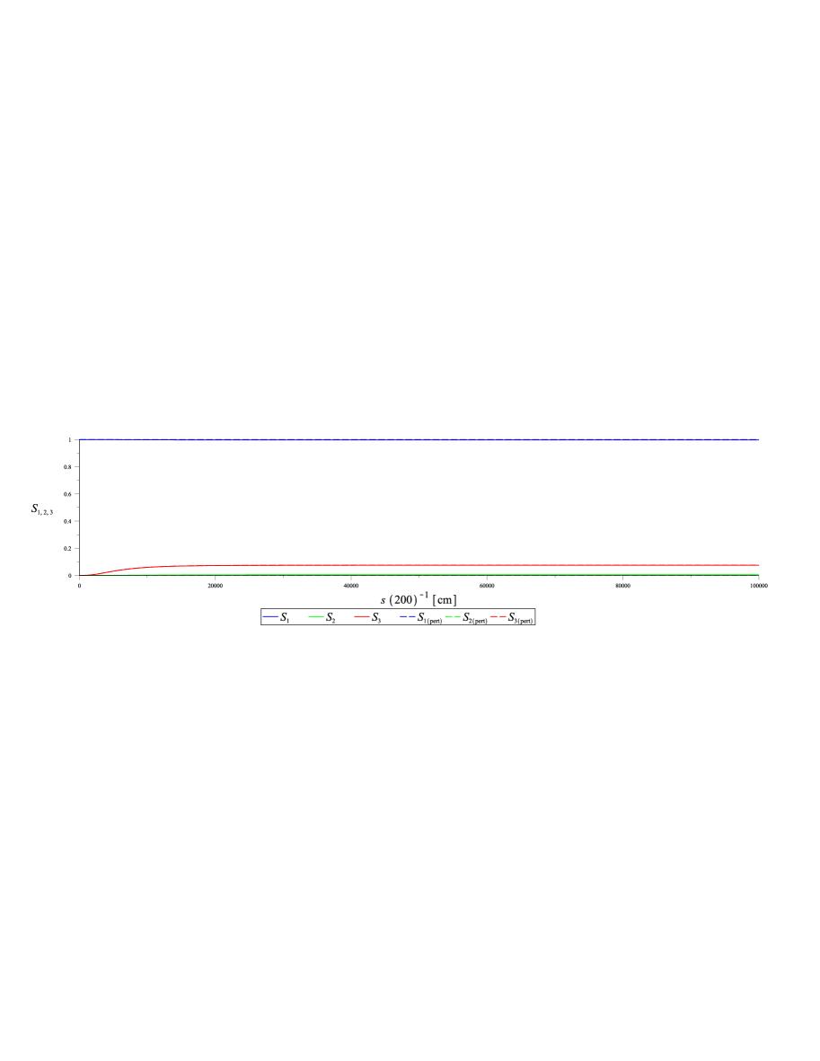
(a) With $\mathbf{S}\left(0\right)=\left(1,0,0\right)$

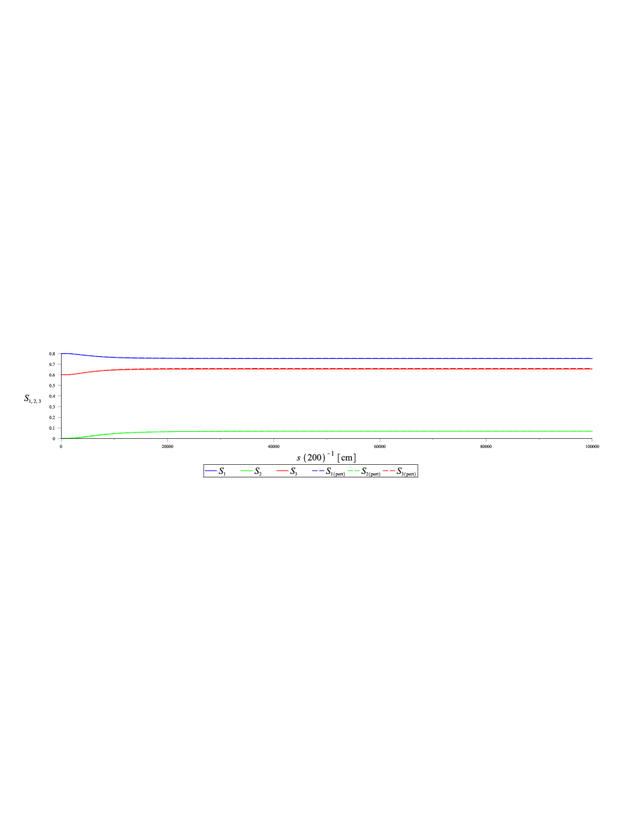
(b) With $\mathbf{S}\left(0\right)=\left(0.8,0,0.6\right)$

Figure 3: Corresponding to Example (i): the evolution of the Stokes vector $\mathbf{S}\left(s\right)=\left(S_{1}\left(s\right),S_{2}\left(s\right),S_{3}\left(s\right)\right)$, $0\leq s\leq 20r_{*}\left(\approx 2\times 10^{7}\,\mathrm{cm}\right)$, for the X-ray emissions from the pulsar with $B_{\mathrm{max}}\approx 10^{12}\,\mathrm{G}$ and $\Omega_{\mathrm{p}}\approx 392.7\,\mathrm{Hz}$ ($P\approx 0.016\,\mathrm{s}$).

Example (ii)

With $B_{\mathrm{max}}\approx 5.6\times 10^{12}\,\mathrm{G}$ and $\Omega_{\mathrm{p}}\approx 22.28\,\mathrm{Hz}$ ($P\approx 0.282\,\mathrm{s}$), we obtain numerical solutions through equations (23)-(25), as shown in Figs. 4a and 4b, given the initial Stokes vectors $\mathbf{S}\left(0\right)=\left(S_{1}\left(0\right),S_{2}\left(0\right),S_{3}\left(0\right)\right)=\left(1,0,0\right)$ and $\left(0.8,0,0.6\right)$, respectively. On the Poincaré sphere, our solutions are represented by the magenta and light blue loci in Fig. 6b, corresponding to Figs. 4a and 4b, respectively. The loci imply about half an oscillation for the polarization evolution, as is confirmed later by the approximate analytical solutions in Section 2.2.2.

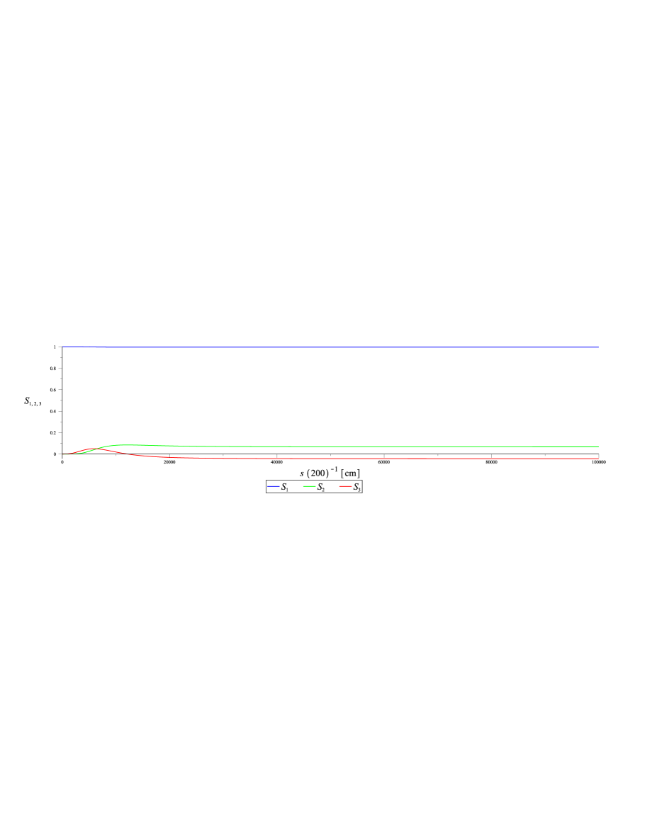
(a) With $\mathbf{S}\left(0\right)=\left(1,0,0\right)$

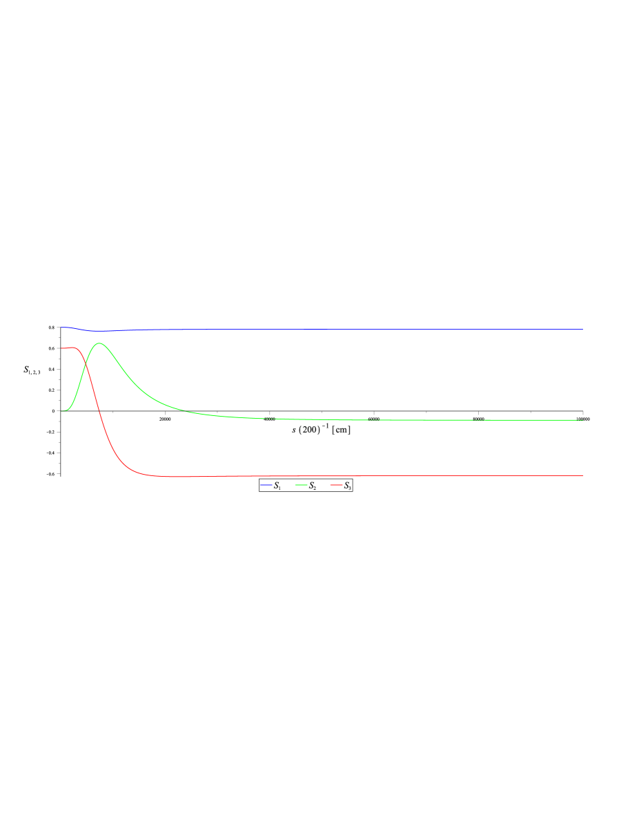
(b) With $\mathbf{S}\left(0\right)=\left(0.8,0,0.6\right)$

Figure 4: Corresponding to Example (ii): the evolution of the Stokes vector $\mathbf{S}\left(s\right)=\left(S_{1}\left(s\right),S_{2}\left(s\right),S_{3}\left(s\right)\right)$, $0\leq s\leq 20r_{*}\left(\approx 2\times 10^{7}\,\mathrm{cm}\right)$, for the X-ray emissions from the pulsar with $B_{\mathrm{max}}\approx 5.6\times 10^{12}\,\mathrm{G}$ and $\Omega_{\mathrm{p}}\approx 22.28\,\mathrm{Hz}$ ($P\approx 0.282\,\mathrm{s}$).

Example (iii)

With $B_{\mathrm{max}}\approx 5.0\times 10^{13}\,\mathrm{G}$ and $\Omega_{\mathrm{p}}\approx 19.6\,\mathrm{Hz}$ ($P\approx 0.32\,\mathrm{s}$), we obtain numerical solutions through equations (23)-(25), as shown in Figs. 5a and 5b, given the initial Stokes vectors $\mathbf{S}\left(0\right)=\left(S_{1}\left(0\right),S_{2}\left(0\right),S_{3}\left(0\right)\right)=\left(1,0,0\right)$ and $\left(0.8,0,0.6\right)$, respectively. On the Poincaré sphere, our solutions are represented by the magenta and light blue loci in Fig. 6c, corresponding to Figs. 5a and 5b, respectively. The loci imply multiple oscillations for the polarization evolution, as is confirmed later by the approximate analytical solutions in Section 2.2.2.

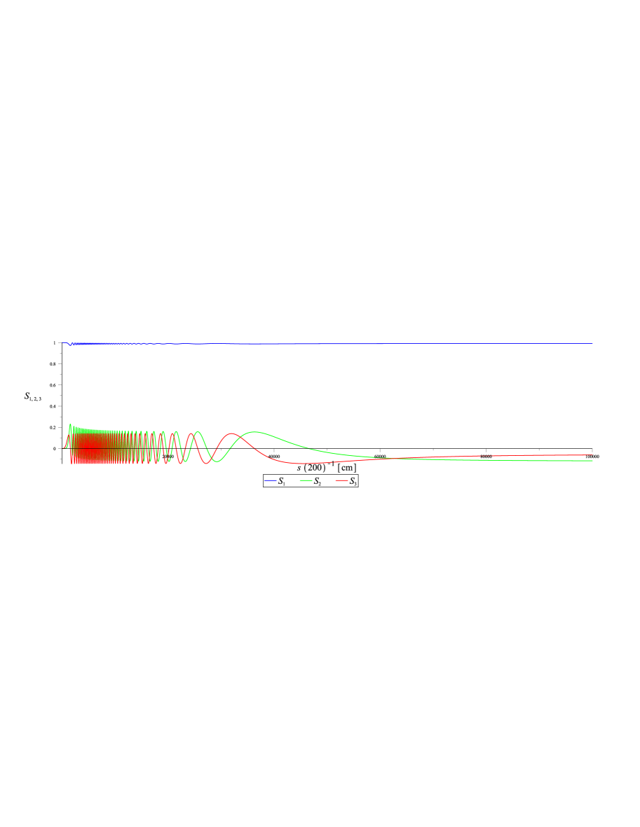
(a) With $\mathbf{S}\left(0\right)=\left(1,0,0\right)$

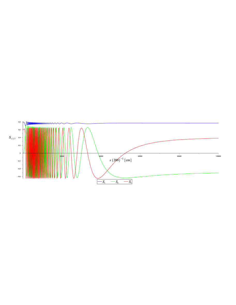
(b) With $\mathbf{S}\left(0\right)=\left(0.8,0,0.6\right)$

Figure 5: Corresponding to Example (iii): the evolution of the Stokes vector $\mathbf{S}\left(s\right)=\left(S_{1}\left(s\right),S_{2}\left(s\right),S_{3}\left(s\right)\right)$, $0\leq s\leq 20r_{*}\left(\approx 2\times 10^{7}\,\mathrm{cm}\right)$, for the X-ray emissions from the pulsar with $B_{\mathrm{max}}\approx 5.0\times 10^{13}\,\mathrm{G}$ and $\Omega_{\mathrm{p}}\approx 19.6\,\mathrm{Hz}$ ($P\approx 0.32\,\mathrm{s}$).

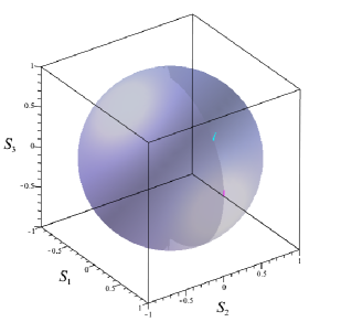
(a) Corresponding to Example (i):
a fraction of an oscillation

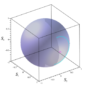
(b) Corresponding to Example (ii):
about half an oscillation

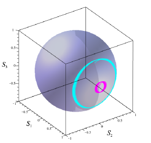
(c) Corresponding to Example (iii):
multiple oscillations

Figure 6: Representations of the Stokes vectors on the Poincaré sphere. The loci imply patterns of the polarization evolution in terms of oscillation.

2.2.2 Approximate analytical solutions

Plotting the birefringent functions $\hat{\Omega}_{1}\left(s\right)$ and $\hat{\Omega}_{2}\left(s\right)$, as given by (18) and (19), respectively, one can observe that they feature distinctive patterns; they can be well approximated by some analytic models, whose curves resemble the original plots. In Fig. 7 are plotted the birefringent functions for the three cases: (a) $B_{\mathrm{max}}\approx 10^{12}\,\mathrm{G}$ and $\Omega_{\mathrm{p}}\approx 392.7\,\mathrm{Hz}$ ($P\approx 0.016\,\mathrm{s}$), (b) $B_{\mathrm{max}}\approx 5.6\times 10^{12}\,\mathrm{G}$ and $\Omega_{\mathrm{p}}\approx 22.28\,\mathrm{Hz}$ ($P\approx 0.282\,\mathrm{s}$), (c) $B_{\mathrm{max}}\approx 5.0\times 10^{13}\,\mathrm{G}$ and $\Omega_{\mathrm{p}}\approx 19.6\,\mathrm{Hz}$ ($P\approx 0.32\,\mathrm{s}$) with solid lines (see Figs. 7a, 7b and 7c, respectively), where they have been evaluated with the same initial condition as assumed in Section 2.2.1.

In correspondence with the actual birefringent functions above, the following analytical models are also plotted with dashed lines in Fig. 7:

$$\hat{\Omega}_{1,2}\left(s\right)\approx-a_{1,2}s^{\frac{p+1}{p}}e^{-bs}~{}~{}\text{for $0\leq s\leq 20r_{*}\left(\approx 2\times 10^{7}\,\mathrm{cm}\right)$},$$ (30)

where $a_{1,2}>0$, $b>0$ and $p>0$ are free parameters; with suitable values chosen for these, our model functions can give rise to solutions of equations (23)-(25) that match fairly well the numerical results obtained in Section 2.2.1. Here we express

$$a_{1,2}=-\hat{\Omega}_{1,2\left(\mathrm{min}\right)}\left[\frac{e}{\left(1-\chi\right)s_{\dagger 1}+\chi s_{\dagger 2}}\right]^{\frac{p+1}{p}},~{}~{}b=\frac{p+1}{p\left[\left(1-\chi\right)s_{\dagger 1}+\chi s_{\dagger 2}\right]},$$ (31)

where $\hat{\Omega}_{1,2\left(\mathrm{min}\right)}=\hat{\Omega}_{1,2}\left(s_{\dagger 1,2}\right)$, evaluated from (18), (19), with $s_{\dagger 1,2}$ denoting the extremum. We have set $p=100$ (a sufficiently large number) for all three cases, and $\chi=0.999$ for (a) and (b), and $\chi=0.056$ for (c) in Fig. 7.

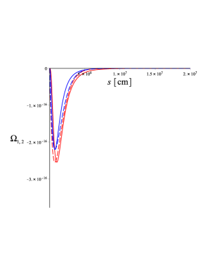
(a) For $B_{\mathrm{max}}\approx 10^{12}\,\mathrm{G}$ and $\Omega_{\mathrm{p}}\approx 392.7\,\mathrm{Hz}$ ($P\approx 0.016\,\mathrm{s}$)

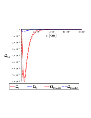
(b) For $B_{\mathrm{max}}\approx 5.6\times 10^{12}\,\mathrm{G}$ and $\Omega_{\mathrm{p}}\approx 22.28\,\mathrm{Hz}$ ($P\approx 0.282\,\mathrm{s}$)

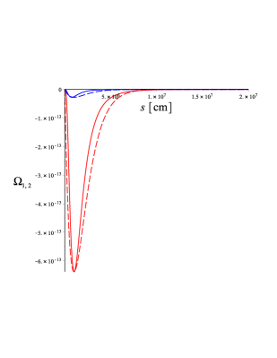
(c) For $B_{\mathrm{max}}\approx 5.0\times 10^{13}\,\mathrm{G}$ and $\Omega_{\mathrm{p}}\approx 19.6\,\mathrm{Hz}$ ($P\approx 0.32\,\mathrm{s}$)

Figure 7: Plots of the birefringent functions $\hat{\Omega}_{1}\left(s\right)$ and $\hat{\Omega}_{2}\left(s\right)$ and their approximate analytic models.

Plugging equation (30) into equations (23)-(25), we obtain analytical solutions as follows (for a complete derivation, see Appendix B):

$$S_{1}\left(s\right) \approx\frac{a_{2}S_{\mathrm{o}}}{\sqrt{a_{1}^{2}+a_{2}^{2}}}\cos\left(\Psi\left(s;p\right)+\delta\right)+\frac{a_{1}C}{\sqrt{a_{1}^{2}+a_{2}^{2}}},$$ (32)

$$S_{2}\left(s\right) \approx-\frac{a_{1}S_{\mathrm{o}}}{\sqrt{a_{1}^{2}+a_{2}^{2}}}\cos\left(\Psi\left(s;p\right)+\delta\right)+\frac{a_{2}C}{\sqrt{a_{1}^{2}+a_{2}^{2}}},$$ (33)

$$S_{3}\left(s\right) \approx S_{\mathrm{o}}\sin\left(\Psi\left(s;p\right)+\delta\right),$$ (34)

where

$$\Psi\left(s;p\right)\equiv k\sqrt{a_{1}^{2}+a_{2}^{2}}b^{-\frac{4p+1}{2p}}s^{\frac{1}{2p}}e^{-\frac{1}{2}bs}\left[M_{\frac{1}{2p},\frac{p+1}{2p}}\left(bs\right)-\left(bs\right)^{\frac{2p+1}{2p}}e^{-\frac{1}{2}bs}\right],$$ (35)

and $M_{\kappa,\mu}\left(z\right)$ denotes a Whittaker function of the first kind, and $a_{1,2}$ and $b$ are given by (31). Here we determine $S_{\mathrm{o}}$, $C$ and $\delta$ by matching the initial value of the Stokes vector $\mathbf{S}\left(0\right)=\left(S_{1}\left(0\right),S_{2}\left(0\right),S_{3}\left(0\right)\right)$ with equations (32)-(34) evaluated at $s=0$.

In Fig. 8 we plot the above solutions for the following cases, assuming $r_{\mathrm{o}}=2r_{*}\approx 2\times 10^{6}\,\mathrm{cm}$, $\theta_{\mathrm{o}}=60^{\circ}$, $\alpha=45^{\circ}$, $\eta\approx 3.97\times 10^{-32}$ for $\hat{\Omega}_{1,2\left(\mathrm{min}\right)}$ (evaluated through (18), (19)) and $\omega\approx 2\pi\times 10^{18}\,\mathrm{Hz}$ ($k\approx 2.0958\times 10^{8}\,\mathrm{cm^{-1}}$) for the X-ray emissions, with the initial Stokes vector $\mathbf{S}\left(0\right)=\left(0.8,0,0.6\right)$:
Case (a) (see Fig. 8a);
for $B_{\mathrm{max}}\approx 10^{12}\,\mathrm{G}$ and $\Omega_{\mathrm{p}}\approx 392.7\,\mathrm{Hz}$ ($P\approx 0.016\,\mathrm{s}$), with the parameters
$\hat{\Omega}_{1\left(\mathrm{min}\right)}\approx-2.5511\times 10^{-16}$, $\hat{\Omega}_{2\left(\mathrm{min}\right)}\approx-2.2054\times 10^{-16}$, $s_{\dagger 1}\approx 1.0202\times 10^{6}\,\mathrm{cm}$, $s_{\dagger 2}\approx 7.5467\times 10^{5}\,\mathrm{cm}$, $p=100$, $\chi=0.999$, $S_{\mathrm{o}}\approx 0.7960$, $C\approx 0.6052$ and $\delta\approx 0.8537$,
Case (b) (see Fig. 8b);
for $B_{\mathrm{max}}\approx 5.6\times 10^{12}\,\mathrm{G}$ and $\Omega_{\mathrm{p}}\approx 22.28\,\mathrm{Hz}$ ($P\approx 0.282\,\mathrm{s}$), with the parameters
$\hat{\Omega}_{1\left(\mathrm{min}\right)}\approx-8.0001\times 10^{-15}$, $\hat{\Omega}_{2\left(\mathrm{min}\right)}\approx-3.9240\times 10^{-16}$, $s_{\dagger 1}\approx 1.0202\times 10^{6}\,\mathrm{cm}$, $s_{\dagger 2}\approx 7.5467\times 10^{5}\,\mathrm{cm}$, $p=100$, $\chi=0.999$, $S_{\mathrm{o}}\approx 0.6013$, $C\approx 0.7990$ and $\delta\approx 1.5056$,
Case (c) (see Fig. 8c);
for $B_{\mathrm{max}}\approx 5.0\times 10^{13}\,\mathrm{G}$ and $\Omega_{\mathrm{p}}\approx 19.6\,\mathrm{Hz}$ ($P\approx 0.32\,\mathrm{s}$), with the parameters
$\hat{\Omega}_{1\left(\mathrm{min}\right)}\approx-6.3776\times 10^{-13}$, $\hat{\Omega}_{2\left(\mathrm{min}\right)}\approx-2.7567\times 10^{-14}$, $s_{\dagger 1}\approx 1.0202\times 10^{6}\,\mathrm{cm}$, $s_{\dagger 2}\approx 7.5467\times 10^{5}\,\mathrm{cm}$, $p=100$, $\chi=0.056$, $S_{\mathrm{o}}\approx 0.6010$, $C\approx 0.7993$ and $\delta\approx 1.5133$.
These plots compare with Figs. 3b (for Example (i)), 4b (for Example (ii)) and 5b (for Example (iii)) in Section 2.2.1, respectively.

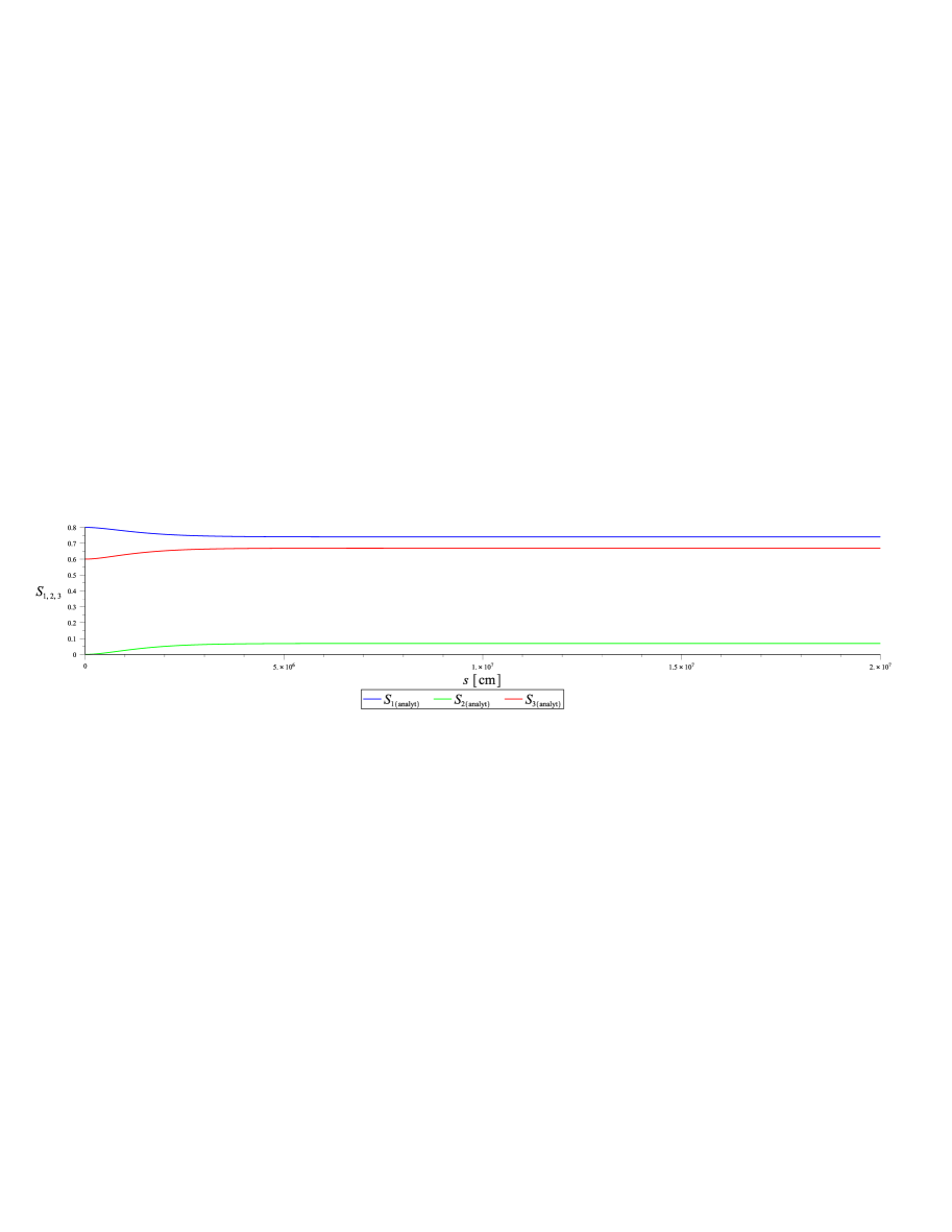
(a) For $B_{\mathrm{max}}\approx 10^{12}\,\mathrm{G}$ and $\Omega_{\mathrm{p}}\approx 392.7\,\mathrm{Hz}$ ($P\approx 0.016\,\mathrm{s}$)

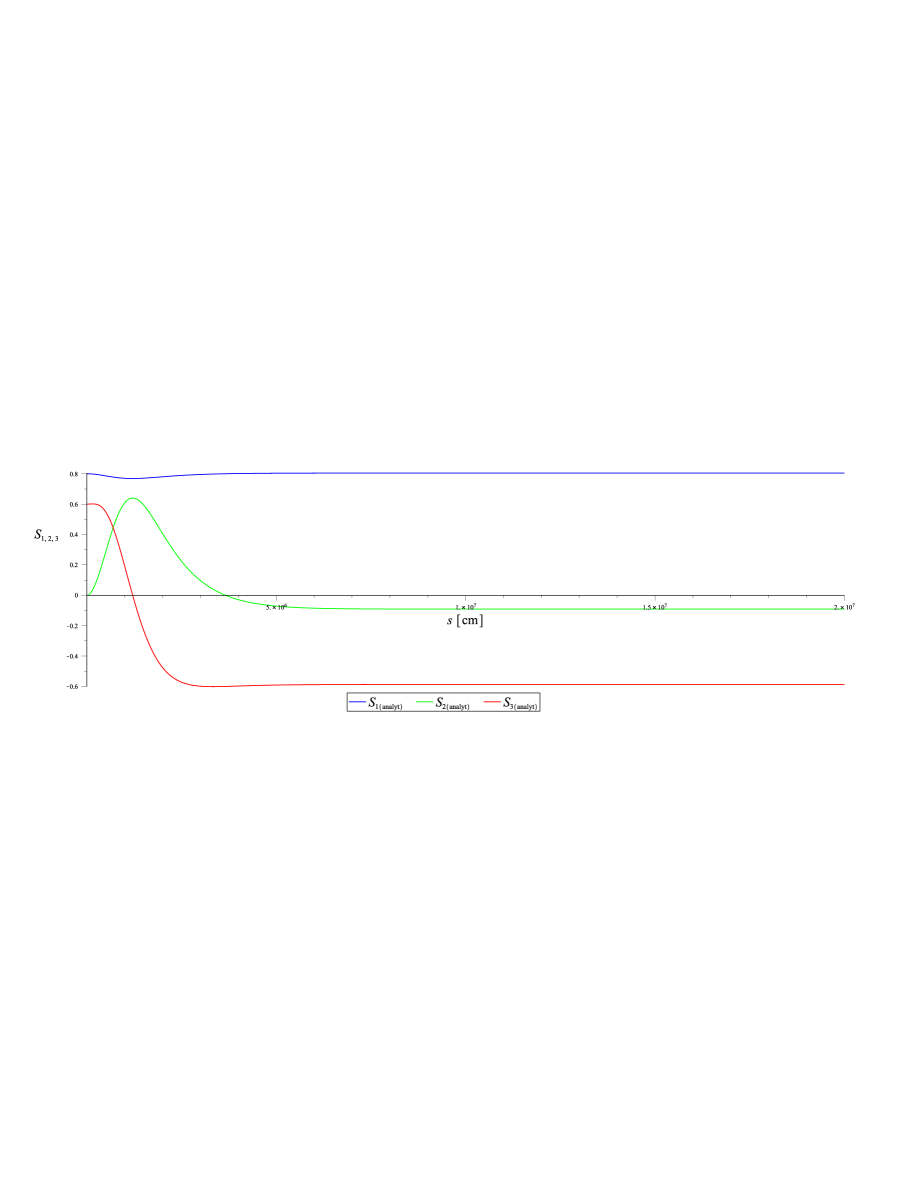
(b) For $B_{\mathrm{max}}\approx 5.6\times 10^{12}\,\mathrm{G}$ and $\Omega_{\mathrm{p}}\approx 22.28\,\mathrm{Hz}$ ($P\approx 0.282\,\mathrm{s}$)

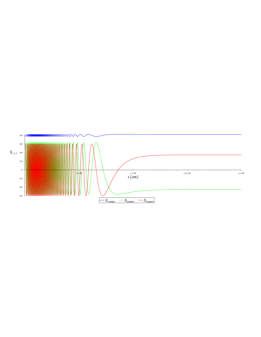
(c) For $B_{\mathrm{max}}\approx 5.0\times 10^{13}\,\mathrm{G}$ and $\Omega_{\mathrm{p}}\approx 19.6\,\mathrm{Hz}$ ($P\approx 0.32\,\mathrm{s}$)

Figure 8: Plots of the analytical solutions $S_{1}\left(s\right)$, $S_{2}\left(s\right)$ and $S_{3}\left(s\right)$, given the initial Stokes vector $\mathbf{S}\left(0\right)=\left(0.8,0,0.6\right)$.

The analytical solutions (32)-(34) provide a useful tool for understanding the different patterns of polarization evolution for the three cases above, as given by Figs. 8a, 8b and 8c. Inspecting numerically the functional argument $\Psi\left(s;p\right)$ given by (35), one can approximate it to a simpler form with the help of (30) and (31):
For $0\leq s\lesssim 2.5\times 10^{6}\,\mathrm{cm}$,

$$\Psi\left(s;p=100\right)=k\sqrt{a_{1}^{2}+a_{2}^{2}}b^{-\frac{401}{200}}s^{\frac{1}{200}}e^{-\frac{1}{2}bs}\left[M_{\frac{1}{200},\frac{101}{200}}\left(bs\right)-\left(bs\right)^{\frac{201}{200}}e^{-\frac{1}{2}bs}\right]\approx 0.24k\sqrt{\hat{\Omega}_{1\left(\mathrm{min}\right)}^{2}+\hat{\Omega}_{2\left(\mathrm{min}\right)}^{2}}\pi s.$$ (36)

Using this, we can estimate how much the oscillations for the three cases have progressed, for example, during $0\leq s\lesssim 1.2\times 10^{6}\,\mathrm{cm}$:

$$\Psi\left(s\approx 1.2\times 10^{6}\,\mathrm{cm};p=100\right) \approx\left\{\begin{array}[]{ll}0.02\pi\hskip 9.0pt\text{(a fraction of an oscillation)}&\hskip 12.0pt\text{for Case (a)},\\ 0.5\pi\hskip 13.0pt\text{(about half an oscillation)}&\hskip 12.0pt\text{for Case (b)},\\ 39\pi\hskip 15.0pt\text{(multiple oscillations)}&\hskip 12.0pt\text{for Case (c)},\end{array}\right.$$ (40)

which can be checked by comparison with Figs. 8a, 8b and 8c, respectively.

Recalling Example (i) from Section 2.2.1, one finds that the condition for perturbation can be equivalently expressed using (36):

$$\left|k\hat{\Omega}_{1,2}\left(s\right)s\right|_{\mathrm{max}}\sim\left|k\hat{\Omega}_{1,2\left(\mathrm{min}\right)}s_{\dagger 1,2}\right|\sim 0.24k\sqrt{\hat{\Omega}_{1\left(\mathrm{min}\right)}^{2}+\hat{\Omega}_{2\left(\mathrm{min}\right)}^{2}}\pi\left(1.2\times 10^{6}\,\mathrm{cm}\right)\approx 0.02\pi\ll 1~{}~{}\text{for Example (i) or Case (a)}.$$ (41)

Extending this argument, similarly to (40) above we may state the following in reference to the patterns of polarization evolution:

$$\left|k\hat{\Omega}_{1,2}\left(s\right)s\right|_{\mathrm{max}}\left\{\begin{array}[]{ll}\ll 1\hskip 9.0pt\text{(fractionally oscillatory - monotonic)}&\hskip 12.0pt\text{for Example (i)},\\ \sim\hskip 2.0pt1\hskip 9.0pt\text{(half oscillatory)}&\hskip 12.0pt\text{for Example (ii)},\\ \gg 1\hskip 9.0pt\text{(highly oscillatory)}&\hskip 12.0pt\text{for Example (iii)}.\end{array}\right.$$ (45)

3 Conclusions and discussion

We have investigated the evolution of polarization states under the quantum refraction effects combined with the frequency dependence of pulsar emission. To this end, we have solved a system of evolution equations of the Stokes vector given by (1) (or by (23)-(25)) for three examples of RPPs at a fixed frequency for specific emissions (e.g., X-rays as in Sections 2.2.1 and 2.2.2). Our main results are presented in Figs. 3-6, from numerical solutions and in part from perturbative solutions. Also, we have approximated the birefringent vector by some models as in Fig. 7 to solve the evolution equations analytically, and obtained the results as presented in Fig. 8, from approximate analytical solutions. It is noteworthy that at a fixed frequency of emission the evolution of the Stokes vector largely exhibits three different patterns, depending on the magnitudes of the birefringent vector, in which the magnetic field strength is a dominant factor: (i) fractionally oscillatory - adiabatic/monotonic, or (ii) half-oscillatory, or (iii) highly oscillatory behaviours. These features are shown by the numerical solutions in Figs. 3-6, and also confirmed by the approximate analytical solutions in Fig. 8.

This study is centred on solving the evolution equations for polarization states (1), wherein the birefringent vector that contains all information about the quantum refraction effects, coupled to the frequency of pulsar emission, acts on the Stokes vector; the evolution results from the combination of the quantum refraction effects and the frequency dependence of the emission. This is a major difference from our previous work (Kim et al. (2024)), wherein the same effects are independent of the emission frequency; the work solely focuses on the quantum refraction effects on the propagation and polarization of a photon from pulsar emission, with no reference to other properties of the emission, such as the frequency. In this regard, it is worthwhile to draw comparison between the two quantities, the polarization vector and the Stokes vector, both of which are used to describe polarization states. The polarization vector is defined directly from the radiative electric field vector (i.e. the unit electric field vector), and it is parallel-transported along the the propagation vector; usually, we consider such two vectors orthogonal to each other and to the propagation vector to define an orthonormal basis consisting of the three vectors. In contrast, the Stokes vector is defined from Stokes parameters which are built out of the radiative electric field vector (Rybicki & Lightman (1991)). The representation of the Stokes vector is abstract in the sense that it is a vector defined on the Poincaré sphere. The Stokes vector is not parallel-transported along the the propagation vector, but can still be defined along the propagation vector as the two polarization vectors move along it; hence, it can be parametrised by $s$ to represent polarization states along the photon trajectory. However, the Stokes vector has a crucial advantage over the polarization vector in representing polarization states in some astrophysical studies like this: it can be directly estimated from polarimetric measurements and accommodate depolarization effects due to incomplete coherence and random processes during the photon propagation (Scully & Zubairy (1997)).

With regard to the adiabatic evolution condition as mentioned in Heyl & Shaviv (2000), Heyl et al. (2003), and Heyl & Caiazzo (2018), we have carefully examined our results presented in Figs. 3-5 to see what interpretations the condition leads to. Solving the condition $\left|k\mathbf{\hat{\Omega}}\left(\mathrm{d}\ln|k\mathbf{\hat{\Omega}}|/\mathrm{d}s\right)^{-1}\right|\gtrsim 0.05$ for $s$ (note that our $k\mathbf{\hat{\Omega}}$ is equivalent to the birefringent vector as defined in the references above and that we have set the condition value to $0.05$ rather than $0.5$ as in the references) yields $s_{\mathrm{PL}1}\lesssim s\lesssim s_{\mathrm{PL}2}$, where $s_{\mathrm{PL}1[2]}$ refers to the lower [upper] bound for the ‘polarization limiting’ distance as measured from the emission point. Using this, we have checked out the following: (1) for $6.2\times 10^{5}\,\mathrm{cm}\lesssim s\lesssim 1.8\times 10^{6}\,\mathrm{cm}$ in Fig. 3, (2) for $3.1\times 10^{5}\,\mathrm{cm}\lesssim s\lesssim 6.2\times 10^{6}\,\mathrm{cm}$ in Fig. 4, (3) for $1.1\times 10^{5}\,\mathrm{cm}\lesssim s\lesssim 1.9\times 10^{7}\,\mathrm{cm}$ in Fig. 5, our Stokes vector evolves evidently; otherwise, it freezes.

Effects of gravitation have not been considered in this study. However, close to the neutron star, where gravitation due to the neutron star mass may not be negligible, its effects must be taken into account in our analysis. Then, basically, the following shall be redefined in curved spacetime: (1) the QED one-loop effective Lagrangian, (2) the refractive index for the photon propagation, (3) the magnetic field geometry in the magnetosphere, (4) the radiative electric field due to a charge moving along a magnetic field line, (5) the photon trajectory. All these have not been rigorously dealt with in previous studies. In this regard, inclusion of the gravitational effects will involve non-trivial and immense analyses, and therefore shall be conducted for a long-term plan in our future studies.

Data Availability

The inclusion of a Data Availability Statement is a requirement for articles published in MNRAS. Data Availability Statements provide a standardised format for readers to understand the availability of data underlying the research results described in the article. The statement may refer to original data generated in the course of the study or to third-party data analysed in the article. The statement should describe and provide means of access, where possible, by linking to the data or providing the required accession numbers for the relevant databases or DOIs.

If you want to present additional material which would interrupt the flow of the main paper, it can be placed in an Appendix which appears after the list of references.

Appendix A The classical Stokes vector

Consider a particle with a charge $q$ moving along a curved trajectory (a magnetic field line). Then the curvature radiation due to this can be expressed by the electric field:

$$\mathbf{E}\left(t\right)=\frac{q}{c\left|\mathbf{r}-\boldsymbol{\xi}\left(t_{\mathrm{ret}}\right)\right|}\frac{\mathbf{n\times}\left[\left(\mathbf{n-}\frac{\dot{\boldsymbol{\xi}}\left(t_{\mathrm{ret}}\right)}{c}\right)\times\frac{\ddot{\boldsymbol{\xi}}\left(t_{\mathrm{ret}}\right)}{c}\right]}{\left(1-\frac{\dot{\boldsymbol{\xi}}\left(t_{\mathrm{ret}}\right)}{c}\cdot\mathbf{n}\right)^{3}},$$ (46)

where $t_{\mathrm{ret}}\equiv t-r/c$ is the retarded time, $\boldsymbol{\xi}$ represents the particle’s trajectory, $\mathbf{n}$ is the propagation direction of the radiation, and an over-dot ${\dot{}}$ denotes differentiation with respect to $t$. In a suitably chosen Cartesian frame, by setting $\boldsymbol{\xi}\left(t_{\mathrm{ret}}\right)=\rho\left(\sin\left(\beta ct_{\mathrm{ret}}/\rho\right),0,\cos\left(\beta ct_{\mathrm{ret}}/\rho\right)\right)$, with $\rho$ being the radius of curvature of the particle’s trajectory, and $\mathbf{n}=\left(\cos\varphi,\sin\varphi,0\right)$, with $\varphi$ being the angle measured from the $x$-axis to the plane of the particle’s motion, we can construct a simple toy model for pulse profiles of pulsar curvature emission as described below (Kim & Trippe (2021)).

One can express Stokes parameters out of the radiation field (46), which describe polarization properties of the curvature radiation (Gil & Snakowski (1990)):

$$I =\tilde{E}_{\parallel}^{\ast}\tilde{E}_{\parallel}+\tilde{E}_{\perp}^{\ast}\tilde{E}_{\perp}$$

$$=\mathcal{E}_{\mathrm{o}}^{2}\omega^{2}\left[\left(\delta^{2}+\varphi^{2}\right)^{2}\mathrm{K}_{2/3}^{2}\left(\frac{\rho\omega}{3\beta c}\left(\delta^{2}+\varphi^{2}\right)^{3/2}\right)+\,\varphi^{2}\left(\delta^{2}+\varphi^{2}\right)\mathrm{K}_{1/3}^{2}\left(\frac{\rho\omega}{3\beta c}\left(\delta^{2}+\varphi^{2}\right)^{3/2}\right)\right],$$ (47)

$$Q =\tilde{E}_{\parallel}^{\ast}\tilde{E}_{\parallel}-\tilde{E}_{\perp}^{\ast}\tilde{E}_{\perp}$$

$$=\mathcal{E}_{\mathrm{o}}^{2}\omega^{2}\left[\left(\delta^{2}+\varphi^{2}\right)^{2}\mathrm{K}_{2/3}^{2}\left(\frac{\rho\omega}{3\beta c}\left(\delta^{2}+\varphi^{2}\right)^{3/2}\right)-\,\varphi^{2}\left(\delta^{2}+\varphi^{2}\right)\mathrm{K}_{1/3}^{2}\left(\frac{\rho\omega}{3\beta c}\left(\delta^{2}+\varphi^{2}\right)^{3/2}\right)\right],$$ (48)

$$U =\tilde{E}_{\parallel}^{\ast}\tilde{E}_{\perp}+\tilde{E}_{\parallel}\tilde{E}_{\perp}^{\ast}=0,$$ (49)

$$V =-\mathrm{i}\left(\tilde{E}_{\parallel}^{\ast}\tilde{E}_{\perp}-\tilde{E}_{\parallel}\tilde{E}_{\perp}^{\ast}\right)$$

$$=-2\mathcal{E}_{\mathrm{o}}^{2}\omega^{2}\varphi\left(\delta^{2}+\varphi^{2}\right)^{3/2}\mathrm{K}_{2/3}\left(\frac{\rho\omega}{3\beta c}\left(\delta^{2}+\varphi^{2}\right)^{3/2}\right)\mathrm{K}_{1/3}\left(\frac{\rho\omega}{3\beta c}\left(\delta^{2}+\varphi^{2}\right)^{3/2}\right),$$ (50)

where $\tilde{E}_{\parallel}$ and $\tilde{E}_{\perp}$ denote the components of the Fourier transform $\mathbf{\tilde{E}}\left(\omega\right)=\tilde{E}_{\parallel}\left(\omega\right)\mathbf{e}_{z}+\tilde{E}_{\perp}\left(\omega\right)\,\mathbf{e}_{y}=\int_{-\infty}^{\infty}\mathbf{E}\left(t\right)\exp\left(\mathrm{i}\omega t\right)\,\mathrm{d}t$, expressed in the Cartesian frame, and ^∗ means the complex conjugate, and $\mathcal{E}_{\mathrm{o}}=q\beta/\left(2\sqrt{3}\pi^{2}r\rho\right)$, and $\delta\equiv\gamma^{-1}=\left(1-\beta^{2}\right)^{1/2}\ll 1$ is the half-angle of the beam emission, and $\mathrm{K}_{1/3}$ and $\mathrm{K}_{2/3}$ denote the modified Bessel functions of the second kind. With regard to the polarization state of the curvature radiation, $I$ is a measure of the total intensity, $Q$ and $U$ jointly describe the linear polarization, and $V$ describes the circular polarization. These parameters can be plotted as functions of the phase angle $\varphi$, where $\varphi\leq\delta\ll 5^{\circ}$ usually, to simulate the pulse profiles of pulsar emission theoretically.

Out of the Stokes parameters, one can define the Stokes vector $\mathbf{S}=\left(S_{1},S_{2},S_{3}\right)\allowbreak\equiv\left(Q/I,U/I,V/I\right)$ and express it using (47)-(50):

$$S_{1} =\frac{\left(\delta^{2}+\varphi^{2}\right)\mathrm{K}_{2/3}^{2}\left(\frac{\rho\omega}{3\beta c}\left(\delta^{2}+\varphi^{2}\right)^{3/2}\right)-\,\varphi^{2}\mathrm{K}_{1/3}^{2}\left(\frac{\rho\omega}{3\beta c}\left(\delta^{2}+\varphi^{2}\right)^{3/2}\right)}{\left(\delta^{2}+\varphi^{2}\right)\mathrm{K}_{2/3}^{2}\left(\frac{\rho\omega}{3\beta c}\left(\delta^{2}+\varphi^{2}\right)^{3/2}\right)+\,\varphi^{2}\mathrm{K}_{1/3}^{2}\left(\frac{\rho\omega}{3\beta c}\left(\delta^{2}+\varphi^{2}\right)^{3/2}\right)},$$ (51)

$$S_{2} =0,$$ (52)

$$S_{3} =-\frac{2\varphi\left(\delta^{2}+\varphi^{2}\right)^{1/2}\mathrm{K}_{2/3}\left(\frac{\rho\omega}{3\beta c}\left(\delta^{2}+\varphi^{2}\right)^{3/2}\right)\mathrm{K}_{1/3}\left(\frac{\rho\omega}{3\beta c}\left(\delta^{2}+\varphi^{2}\right)^{3/2}\right)}{\left(\delta^{2}+\varphi^{2}\right)\mathrm{K}_{2/3}^{2}\left(\frac{\rho\omega}{3\beta c}\left(\delta^{2}+\varphi^{2}\right)^{3/2}\right)+\,\varphi^{2}\mathrm{K}_{1/3}^{2}\left(\frac{\rho\omega}{3\beta c}\left(\delta^{2}+\varphi^{2}\right)^{3/2}\right)}.$$ (53)

In Fig. 9 is plotted the classical Stokes vector against the phase angle $\varphi$, where we have set, for example, $\delta\approx 10^{-8}$, $\rho\approx 10^{8}\,\mathrm{cm}$, $\beta\approx 1$ and $\omega\approx 2\pi\times 10^{18}\,\mathrm{Hz}$ to model pulse profiles of X-ray pulsar emission. Here the initial values for the Stokes vector, $\mathbf{S}\left(\varphi=0\right)=\left(1,0,0\right)$ and $\mathbf{S}\left(\varphi\approx-1.16\times 10^{-6}\,\mathrm{rad}\right)=\left(0.8,0,0.6\right)$, as in the examples given in Section 2.2.1, are marked by solid circles and solid boxes, respectively.

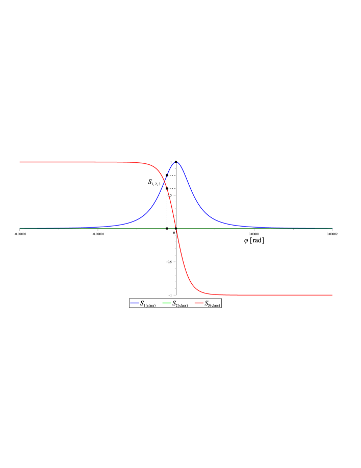
Figure 9: The classical Stokes vector $\mathbf{S}\left(\varphi\right)=\left(S_{1}\left(\varphi\right),S_{2}\left(\varphi\right),S_{3}\left(\varphi\right)\right)$ plotted against the phase angle $\varphi$. Its initial values $\mathbf{S}\left(\varphi=0\right)=\left(1,0,0\right)$ and $\mathbf{S}\left(\varphi\approx-1.16\times 10^{-6}\,\mathrm{rad}\right)=\left(0.8,0,0.6\right)$ are marked by solid circles and solid boxes, respectively.

Appendix B Approximate analytical solutions to evolution equations

Substituting equation (30) into equations (23)-(25), the evolution equations can be reduced as follows:
For $0\leq s\leq 20r_{*}$,

$$\dot{S}_{1}\left(s\right)\approx-ka_{2}s^{\frac{p+1}{p}}e^{-bs}S_{3}\left(s\right),$$ (54)

$$\dot{S}_{2}\left(s\right)\approx ka_{1}s^{\frac{p+1}{p}}e^{-bs}S_{3}\left(s\right),$$ (55)

$$\ddot{S}_{3}\left(s\right)-\left(\frac{p+1}{ps}-b\right)\dot{S}_{3}\left(s\right)+k^{2}\left(a_{1}^{2}+a_{2}^{2}\right)\left(s^{\frac{p+1}{p}}e^{-bs}\right)^{2}S_{3}\left(s\right)\approx 0.$$ (56)

First, we solve equation (56) for $S_{3}\left(s\right)$, and then using this solution, obtain $S_{1}\left(s\right)$ and $S_{2}\left(s\right)$, by integrating equations (54) and (55), respectively:

$$S_{3}\left(s\right) \approx S_{\mathrm{o}}\sin\left(\Psi\left(s;p\right)+\delta\right),$$ (57)

$$S_{1}\left(s\right) \approx\frac{a_{2}S_{\mathrm{o}}}{\sqrt{a_{1}^{2}+a_{2}^{2}}}\cos\left(\Psi\left(s;p\right)+\delta\right)+S_{1\mathrm{o}},$$ (58)

$$S_{2}\left(s\right) \approx-\frac{a_{1}S_{\mathrm{o}}}{\sqrt{a_{1}^{2}+a_{2}^{2}}}\cos\left(\Psi\left(s;p\right)+\delta\right)+S_{2\mathrm{o}},$$ (59)

where

$$\Psi\left(s;p\right)\equiv k\sqrt{a_{1}^{2}+a_{2}^{2}}b^{-\frac{4p+1}{2p}}s^{\frac{1}{2p}}e^{-\frac{1}{2}bs}\left[M_{\frac{1}{2p},\frac{p+1}{2p}}\left(bs\right)-M_{\frac{2p+1}{2p},\frac{p+1}{2p}}\left(bs\right)\right],$$ (60)

and $M_{\kappa,\mu}\left(z\right)$ denotes a Whittaker function of the first kind. Here employing the identity $S_{1}^{2}\left(s\right)+S_{2}^{2}\left(s\right)+S_{3}^{2}\left(s\right)=1$ (conservation of the degree of polarization), one can specify $S_{1\mathrm{o}}$ and $S_{2\mathrm{o}}$ in terms of $a_{1}$, $a_{2}$ and a constant $C$, and establish a relation between $S_{\mathrm{o}}$ and $C$:

$$S_{1\mathrm{o}}=\frac{Ca_{1}}{\sqrt{a_{1}^{2}+a_{2}^{2}}},~{}~{}S_{2\mathrm{o}}=\frac{Ca_{2}}{\sqrt{a_{1}^{2}+a_{2}^{2}}},~{}~{}S_{\mathrm{o}}^{2}+C^{2}=1.$$ (61)

Then $S_{\mathrm{o}}$, $C$ and $\delta$ are determined by matching the initial value of the Stokes vector $\mathbf{S}\left(0\right)=\left(S_{1}\left(0\right),S_{2}\left(0\right),S_{3}\left(0\right)\right)$ with equations (57)-(59) evaluated at $s=0$.

References

- Blandford & Payne (1982) Blandford R. D., Payne D. G., 1982, MNRAS, 199, 883
- Ejlli et al. (2020) Ejlli A., Della Valle F., Gastaldi U., Messineo G., Pengo R., Ruoso G., Zavattini G., 2020, Phys. Rept., 871, 1
- Fedotov et al. (2023) Fedotov A., Ilderton A., Karbstein F., King B., Seipt D., Taya H., Torgrimsson G., 2023, Phys. Rept., 1010, 1
- Gangadhara (2005) Gangadhara R. T., 2005, ApJ, 628, 923
- Gil & Snakowski (1990) Gil J. A., Snakowski J. K., 1990, Astronomy and Astrophysics, 234, 237
- Harding & Lai (2006) Harding A. K., Lai D., 2006, Rep. Prog. Phys., 69, 2631
- Hattori et al. (2023) Hattori K., Itakura K., Ozaki S., 2023, Prog. Part. Nucl. Phys., 133, 104068
- Heisenberg & Euler (1936) Heisenberg W., Euler H., 1936, Zeitschr. Phys, 98, 714
- Heyl & Caiazzo (2018) Heyl J., Caiazzo I., 2018, Galaxies, 6, 76
- Heyl & Shaviv (2000) Heyl J. S., Shaviv N. J., 2000, MNRAS, 311, 555
- Heyl et al. (2003) Heyl J. S., Shaviv N. J., Lloyd D., 2003, MNRAS, 342, 134
- Kim & Kim (2021) Kim C. M., Kim S. P., 2021, Magnetars as Laboratories for Strong Field QED (arXiv:2112.02460)
- Kim & Trippe (2021) Kim D.-H., Trippe S., 2021, General relativistic effects on pulsar radiation (arXiv:2109.13387)
- Kim et al. (2024) Kim D.-H., Kim C. M., Kim S. P., 2024, Monthly Notices of the Royal Astronomical Society, 531, 2148
- Kubo & Nagata (1981) Kubo H., Nagata R., 1981, J. Opt. Soc. Am., 71, 327
- Kubo & Nagata (1983) Kubo H., Nagata R., 1983, J. Opt. Soc. Am., 73, 1719
- Kubo & Nagata (1985) Kubo H., Nagata R., 1985, J. Opt. Soc. Am. A, 2, 30
- Meszaros (1992) Meszaros P., 1992, High-energy radiation from magnetized neutron stars. The University Of Chicago Press, Chicago
- NIST (2024) NIST 2024, Digital Library of Mathematical Functions, National Institute of Standards and Technology, U.S. Department of Commerce, https://dlmf.nist.gov
- Novak et al. (2018) Novak O., Diachenko M., Padusenko E., Kholodov R., 2018, Ukrainian Journal of Physics, 63, 979
- Pavlov et al. (2013) Pavlov G., Kargaltsev O., Durant M. Posselt B., 2013, X-ray Observations of Rotation Powered Pulsars, https://www.cosmos.esa.int/documents/332006/943890/GPavlov_t.pdf
- Raffelt (1996) Raffelt G. G., 1996, Stars as laboratories for fundamental physics : the astrophysics of neutrinos, axions, and other weakly interacting particles. The University Of Chicago Press, Chicago, https://ui.adsabs.harvard.edu/abs/1996slfp.book.....R
- Ruffini et al. (2010) Ruffini R., Vereshchagin G., Xue S.-S., 2010, Phys. Rept., 487, 1
- Rybicki & Lightman (1991) Rybicki G. B., Lightman A. P., 1991, Radiative processes in astrophysics. John Wiley & Sons
- Santangelo et al. (2019) Santangelo A., et al., 2019, Sci China-Phys Mech Astron, 62, 1
- Schwinger (1951) Schwinger J., 1951, Phys. Rev., 82, 664
- Scully & Zubairy (1997) Scully M. O., Zubairy M. S., 1997, Quantum optics. Cambridge University Press
- Wadiasingh et al. (2019) Wadiasingh Z., et al., 2019, Bull. Am. Astron. Soc., 51
- Yoon et al. (2021) Yoon J. W., Kim Y. G., Choi I. W., Sung J. H., Lee H. W., Lee S. K., Nam C. H., 2021, Optica, 8, 630