A modular entanglement-based quantum computer architecture

Abstract

We propose a modular quantum computation architecture based on utilizing multipartite entanglement. Each module consists of a small-scale quantum computer comprising data, memory and interaction qubits. Interaction qubits are used to selectively couple different modules by enhancing interaction strengths via properly adjusting their internal quantum state, where some non-controllable, distance-dependent coupling is used. In this way, different multipartite entangled states with specific entanglement structures shared between modules are generated, and stored in memory qubits. These states are utilized to deterministically perform certain classes of gates or circuits between modules on demand, including parallel controlled-Z gates with arbitrary interaction patterns, multi-qubit gates or whole Clifford circuits, depending on their entanglement structure. The usage of different kinds of multipartite entanglement rather than Bell pairs allows for more efficient and flexible coupling between modules, leading to a scalable quantum computation architecture.

I Introduction

Quantum computers promise to tackle fundamental and practical problems in science, optimization, logistics, finances, chemistry, and material design that are not accessible with classical devices. However, a large number of qubits is required to harness the full power of quantum computers. Small-scale processors as are available now are already at the edge of outperforming classical devices [1, 2, 3, 4], but due to the exponentially growing state space of quantum devices, their power is supposed to grow exponentially with system size. Scaling up quantum computers to make them applicable to real-world problems is thus a crucial, though challenging task. Modular architectures [5, 6, 7, 8] have been identified to be one possible solution, where small-scale processors are coupled and enabled to interact. Different ways to facilitate interactions and gates between modules have been proposed. This includes the shuttling of ions to some interaction zone [9, 10, 11, 8], or the usage of microwave links, waveguides or optical fibres [12, 13, 14]. Auxiliary entanglement that is generated and possibly purified [15, 16, 17] can be utilized to perform gates between modules, which has the advantage that also probabilistic, low-fidelity couplings between modules suffice. What all proposals so far have in common is that they are based on bipartite entanglement, and use tunable interactions or actual transmission of particles, photons or phonons.

Here we propose a modular quantum computation architecture with two distinct features: First, we use an alternative way of coupling modules that does not rely on controlling interactions or exchanging particles but uses some (possibly weak) distance-dependent coupling that is enhanced by using multiple qubits in each module to generate an effective, strong coupling between multiple qubits that form a logical system. By properly choosing their internal state, interaction strengths between modules can be selectively enhanced or diminished [18, 19, 20], thereby allowing the generation of selectable multipartite entangled states. Second, our approach uses entanglement to interconnect the modules by generalising the two-qubit register scheme [21, 22]. Each module contains several memory qubits in multipartite entangled states of different kinds which are used to implement on-demand different classes of gates or whole circuits between modules. This includes for instance parallel controlled-Z gates with arbitrary pairwise interaction patterns, multiqubit operations, Toffoli gates, or even the implementation of whole circuits composed of arbitrary sequences of Clifford gates in a single run. The latter is a feature of measurement-based computation [23, 24, 25] that we bring to such distributed settings, where an entangled state of size $2n$ suffices to perform an arbitrary Clifford circuit acting on $n$ qubits. In addition, we propose to store different kinds of entangled states in the memory qubits of a memory unit. These states can be used on demand and then regenerated using the interaction qubits of the entangling unit. The fidelity of these states –and hence of the resulting multi-qubit operations– can be enhanced using entanglement purification, i.e., generating multiple copies and processing them. In this way, data qubits in the local processing units can be processed, and high-fidelity gates between different modules can be implemented (see Fig. 1) deterministically. Notice that the approach is platform-independent, and is applicable to various set-ups.

In the following, we describe our proposal in more detail. In Sec. II we introduce the general set-up and describe the processing, entangling and memory units of the modules. In Sec. IV we show how to enhance interactions and generate entanglement between modules. We assume some weak, non-tunable interaction between the physical systems of different modules, and describe how using logical systems comprised of multiple qubits allows one to quadratically enhance effective interaction strength via the choice of internal states. We describe in Sec. V how different kinds of multipartite entangled states can be used as a resource to perform multiple gates or whole circuits between modules. We summarize and conclude in Sec. VI.

II Modular architecture and functionality

In a modular quantum computer, the quantum processor is divided into autonomous modules. Each module consists of a moderated size fully controllable multiqubit system, small enough such that full control within a module can be assumed. The central challenge is how to interconnect the modules to access the full computational capacity of the setting.

To interconnect the modules our quantum computing architecture uses multipartite entanglement which can be used as a resource to implement intermodular operations. With that purpose, in addition to the elementary processing unit, two auxiliary units are hosted in each module, see Fig. 1. The memory unit stores entangled states shared among the other modules. In this approach the implementation of multipartite gates between modules consumes entanglement. For that reason, each module includes a entangling generator unit dedicated to the distribution of entangled states among the modules. In the following, we detail the functionality of each unit.

II.1 Elementary processing unit

The state of the whole quantum processor is encoded in the so-called data qubits, which are distributed between the different modules. In particular, the components hosting the data qubits are small quantum processors called elementary processing units. Despite operations within each module being easy to implement, intermodular connectivity is not direct and it requires the other two units.

II.2 Entangling unit

The entangling unit is the component that couples to the other modules and allows one to implement intermodular gates and generate entanglement between them. Various physical settings could play this role, such as optical fibres connecting the modules [12, 13, 14] or moving atoms to induce interactions between different modules [26, 10, 11, 27, 28, 9]. In our architecture, we envision using physical systems inherently subjected to commuting long-range distant-dependent interactions, e.g., collective interactions induced by laser pulses [29, 30, 31, 32, 33] or dipole-dipole interactions [34, 35, 36, 37, 38]. Each entangling unit consists of a multiqubit system affected by two-body ZZ distance-dependent interactions. To compensate for the distance between modules, all the qubits in each module are used to implement a single logical qubit, which effectively increases the interaction strength between modules. In particular, we obtain a quadratically scaling with the number of physical systems in each entangling unit. This allows us to couple the entangling units in different modules even over large distances and use such interactions to prepare different entangled states between the modules.

While the entangling unit allows us to directly implement multiqubit gates between different modules, we use it to establish different entangled states between the modules, which can be used as a resource to implement multiqubit gates. In this way, the entangling units can run in parallel to the other components generating different entangled states which are eventually stored until required, helping to speed up the whole computation.

II.3 Memory unit

The memory unit acts as an auxiliary quantum processor. The memory qubits are used to store the multipartite states, prepared in the entangling unit. The memory unit is also used to pre-process the entangled states. On the one hand, we use it for reducing potential noise in the entangled states by using multipartite entanglement purification protocols [39, 40, 41, 42]. A memory unit can also be used as a repeater node to interconnect two distant nodes [43, 44]. On the other hand, the states are processed to encode different multiqubit unitary operations that eventually will be implemented to the data qubits in different modules. It is noteworthy that while deterministic implementation of intermodular gates is restricted to Clifford gates, any arbitrary quantum computation can be systematically decomposed into a combination of Clifford operations and single-qubit operations. Such decomposition allows for the implementation of any quantum algorithm.

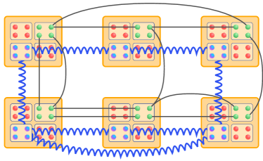
Fig. 1: Each module consists of three components: the elementary processing unit (red qubits), the memory unit (green qubits) and the entangling unit (blue qubits).

III Features of the architecture

In this section, we summarize the features and advantages of our modular architecture, based on two elements. On the one hand, distant-dependent interactions are used to couple the modules. On the other hand, multipartite entangled states shared between the modules are used to implement multiqubit gates.

Tuning and controlling interactions in a many-body system is technically demanding. Here, we do not require direct control of the interactions but only assume an inherent always-on interaction between the qubits hosted in the entangling unit. We use the constituting qubits in each unit to encode a logical qubit that couple to each other. In this way, we obtain stronger interaction strengths, allowing us to couple modules over larger distances. In addition, control over the interaction between the logical qubits is obtained just by manipulating the individual components, which we can use to establish different interaction patterns.

Even though the entangling units could be used directly to implement intermodular qubit gates, we use them to distribute entangled states between the modules. Such states store an intermodular gate that can be locally implemented to the data qubits. In this way, we can parallelize parts of the computation, and mitigate the errors in the intermodular gates by purifying the entangled states.

The architectural design is flexible and not tied to any specific module geometry. Varying arrangements of the modules can result in distinct functionalities. For instance, a larger central module could be specifically designed to facilitate interactions among other modules, whereas smaller modules may excel in processing quantum data or managing entanglement. It’s crucial to select a geometry that optimally distributes entanglement, although the entanglement topologies of the setting is independent by the underlying module geometry.

IV Entanglement generation between modules

It is known [45, 46] that an $n$-qubit system subjected to two-body ZZ interactions, i.e., a Hamiltonian of the form

$$H=\sum_{1\leq i<j\leq n}f_{ij}\,Z_{i}Z_{j},$$

assisted with individual control over the qubit systems allows one to prepare an arbitrary entangle state, i.e., any $n$-qubit state can written as

$$\left|\psi\right\rangle=\prod_{k}\left(e^{\text{i}\lambda_{k}H}\,\bigotimes_{i=1}^{n}L^{(k,i)}\right)\left|0\right\rangle^{\otimes n},$$

where $L^{(k,i)}$ is a single qubit operation and $\lambda_{k}$ an arbitrary parameter.

Therefore, if the qubits of the entangling units are coupled with each other with an interaction of this kind, any quantum circuit can be implemented and, hence, we can distribute any entangled state between the modules. However, the most natural scenario is given when the strength of the interaction decreases with the distance between the two physical systems $d_{ij}$ [34, 31, 32, 37], i.e., $f_{ij}=J/d_{ij}^{\gamma}$ where $\gamma>0$ and $J$ is the coupling constant. Such dependence on the distance impedes using such interactions for coupling the modules, as the interaction strength between two distant modules would be too weak. Nonetheless, this problem can be overcome by increasing the size of the entangling unit.

IV.1 Increasing interaction strengh

If the entangling unit of the $i$th module consists of $m_{i}$ qubits, the interaction between the $i$th and the $j$th module is given by

$$H_{ij}=\sum_{\begin{subarray}{c}1\leq\mu\leq m_{i}\\ 1\leq\nu\leq m_{j}\end{subarray}}f_{i(\mu),j(\nu)}\,Z_{i(\mu)}\,Z_{j(\nu)}$$ (1)

where $f_{i(\mu),j(\nu)}>0$ is the interaction strength between the $\mu$th qubit of the $i$th module and the $\nu$th qubit of the $j$th module (the Latin index labels the module and the Greek index the qubit).

In each entangling unit we implement a logical qubit by restricting its state into the so-called trivial logical subspace spanned by $\left|\bar{0}\right\rangle=\left|0\right\rangle^{\otimes m_{i}}$ and $\left|\bar{1}\right\rangle=\left|1\right\rangle^{\otimes m_{i}}$, in the logical subspace, the interaction Hamiltonian given in Eq. (1) can be written as

$$\bar{H}_{ij}=\sum_{k,k^{\prime},l,l^{\prime}=0}^{1}\left\langle\bar{k}\bar{l}\right|H_{ij}\left|\bar{k}^{\prime}\bar{l}^{\prime}\right\rangle\left|\bar{k}\bar{l}\right\rangle\!\left\langle\bar{k}^{\prime}\bar{l}^{\prime}\right|=\bar{f}_{ij}\,\bar{Z}_{i}\bar{Z}_{j}$$ (2)

where $\bar{Z}=\left|\bar{0}\right\rangle\!\left\langle\bar{0}\right|-\left|\bar{1}\right\rangle\!\left\langle\bar{1}\right|$ and

$$\bar{f}_{ij}=\sum_{\begin{subarray}{c}1\leq\mu\leq m_{i}\\ 1\leq\nu\leq m_{j}\end{subarray}}f_{i(\mu),j(\nu)}$$

is the effective coupling strength between the $i$th and the $j$th logical qubits. As we assume that the distance between physical systems within a module is much smaller than the distance between modules, we approximate $f_{i(\mu),j(\nu)}\approx J/\Delta^{\gamma}_{ij}$, where $\Delta_{ij}$ is the distance between the $i$th and the $j$th module, and then $\bar{f}_{ij}\approx m_{i}\,m_{j}J/\Delta^{\gamma}$. Therefore, note that we obtain the interaction strength between modules increases quadratically with the number of qubits $m_{i}$ in each entangling unit. This enhancement can compensate for the drop in interaction strength due to the distance between the modules, enabling the establishment of strong interactions between distant modules by increasing the size of the entangling units.

IV.2 Interactions control

The trivial subspace is not the only one that simplifies $H_{ij}$ to a logical ZZ interaction, i.e., if we encode a logical qubit in the entangling unit of the $i$th module as $\left|\bar{0}\right\rangle=\left|\boldsymbol{k}_{i}\right\rangle$ and $\left|\bar{1}\right\rangle=X^{\otimes m_{i}}\left|\boldsymbol{k}_{i}\right\rangle$ where $\left|\boldsymbol{k}_{i}\right\rangle$ is a state of the computational basis given by $Z_{i(\mu)}\left|\boldsymbol{k}_{i}\right\rangle=s_{i(\mu)}\left|\boldsymbol{k}_{i}\right\rangle$ and $s_{i(\mu)}=1-2k_{i(\mu)}$ the Hamiltonian is also simplified to Eq. (2). However, in this case, the coupling strength is given by $\bar{f}_{ij}=\sum_{\mu,\nu}f_{i(\mu),j(\nu)}s_{i(\mu)}s_{j(\nu)}$. In Ref. [19] we show how by a suitable choice of the logical subspace of each module, the interaction pattern can be modified establishing arbitrary interaction patterns between the logical systems. However, using a different subspace would lead to a reduction of the coupling strength between the logical qubits. For that reason, for each interaction pattern, the maximum interaction strength needs to be evaluated. In any case, any interaction pattern can be built using the trivial subspace in a “bang-bang” approach, where two interacting logical qubits are encoded in the trivial subspace while the others are encoded in an insensitive subspace, see Ref. [19]. In addition, the trivial encoding improves the fidelity interaction in the presence of thermal noise. As we show in Ref. [20], by a suitable choice of the logical subspace, the fidelity can be further enhanced at the price of a weaker coupling.

Moreover, by encoding a logical qubit in each entangling unit, we make them insensitive to the interactions between its constituents, meaning that the state of the logical qubit is not affected by the interaction of the physical qubits encoding it. This is because any logical subspace of this kind defines a decoherence-free subspace of a ZZ-type interaction, i.e., the internal interactions of the $i$th module are described by $H_{i}=\sum_{\mu<\nu}f_{i(\mu),i(\nu)}Z_{i(\mu)}Z_{i(\nu)}$ and on a logical subspace it simplifies to $\bar{H}_{i}\propto\bar{\mathbbm{1}}$.

Therefore, once a logical qubit is encoded in each entangling unit, the Hamiltonian of the whole system is given by

$$\bar{H}=\sum_{1\leq i<j\leq n}\bar{f}_{ij}\,\bar{Z}_{i}\bar{Z}_{j},$$ (3)

where $\left\{\bar{f}_{ij}\right\}$ can be tuned by a proper choice of the logical subspaces $\{\boldsymbol{k}_{i}\}$. The interaction pattern is described with a graph $\mathcal{G}$ given by a set of $n$ vertices representing the logical qubits and a set of edges $\{(i,j)\}$ between the nodes representing the interaction strength $\bar{f}_{ij}$.

IV.3 State storage

As we showed at the beginning of this section, such an entangling Hamiltonian allows us to prepare the entangling units in any entangled state $\left|\psi\right\rangle$. By implementing a local routine, the state can be transferred to the memory units of the respective modules. The routine consists in first entangling each memory qubit with the logical qubit in its module and then measuring the qubits of the entangling unit on the $X$ basis, i.e., if the logical qubits are encoded in the trivial subspace then

$$\bigotimes_{i=1}^{n}S_{E_{i}\to M_{i}}\!\!:\;\left|\bar{\psi}\right\rangle_{E_{1}\dots E_{n}}\left|\boldsymbol{0}\right\rangle_{M_{1}\dots M_{n}}\mapsto\left|\psi\right\rangle_{M_{1}\dots M_{n}}$$

where $\left|\psi\right\rangle$ is an arbitrary $n$-qubit state, $M_{i}$ labels a memory qubit of the $i$th module, $E_{i}=E_{i(1)}\dots E_{i(m_{i})}$ labels the $m_{i}$-qubit system of the entangling unit of the $i$th module, and

$$S_{E_{i}\to M_{i}}=Z_{M_{i}}^{k_{1}+\dots+k_{m_{i}}}\,O^{(\boldsymbol{k})}_{E_{i}}\,\text{H}^{\otimes m_{i}}_{E_{i}}\,\text{CX}_{E_{i(1)}\to M_{i}}$$

where $O^{(\boldsymbol{k})}=\left|\boldsymbol{k}\right\rangle\!\left\langle\boldsymbol{k}\right|$ and $\text{H}=\left|+\right\rangle\!\left\langle 0\right|+\left|-\right\rangle\!\left\langle 1\right|$ is the Hadamard gate.

V Intermodular gate induction

In the previous section, we demonstrated how using the entangling units we can control an entangling Hamiltonian and prepare arbitrary entangled states between the different modules. The main idea of our architecture is to encode multiqubit gates in multipartite states shared by the modules. These states are used in a later stage to locally perform the corresponding gate to the data qubits of the different modules [47].

V.1 Diagonal gates

First, we analyse the implementation of diagonal gates. A diagonal $n$-qubit gate $\Lambda$ can be stored in an $n$-qubit quantum register by preparing its gate state

$$\left|\Lambda\right\rangle=\Lambda\left|+\right\rangle^{\otimes n}.$$

If we distribute the gate state $\left|\Lambda\right\rangle$ between the memory qubits in different modules, by applying local routine $T$, we can induce $\Lambda$ up to a random byproduct of local $X$ gates to the data qubits of the respective modules. $T$ consists in applying a multilateral control gate between the memory and the data qubits followed by a projective measurement on the memory units. If the measurement outcome on the $i$th memory qubit is given by $k_{i}\in\{0,1\}$, $T$ implements

$$T^{(\boldsymbol{k})}_{\textit{MD}}\left|\Lambda\right\rangle_{M}\left|\psi\right\rangle_{D}\mapsto X^{\otimes\boldsymbol{k}}\,\Lambda\,X^{\otimes\boldsymbol{k}}\left|\psi\right\rangle_{D},$$

to the data qubits, where $T^{(\boldsymbol{k})}_{\textit{MD}}=O^{(\boldsymbol{k})}_{M}\bigotimes_{i=1}^{n}\text{CX}_{D_{i}\to M_{i}}$, $X^{\otimes\boldsymbol{k}}=X^{k_{1}}\otimes\cdots\otimes X^{k_{n}}$. Notice all measurement outcomes are equally probable meaning each possible value of $\boldsymbol{k}$ is given with probability $p=2^{-n}$, see datils in Appendix. B.

Therefore, $T$ only implements $\Lambda$ if $\boldsymbol{k}=\boldsymbol{0}$ is obtained. However, for the so-called Clifford gates, $\Lambda$ can always be implemented by performing a local correction operation. On the other hand, for arbitrary gates, the routine can be used as an elementary step to build a (quasi-)deterministic protocol to induce the gate. At this point, we analyse the implementation of both kinds of gates in detail.

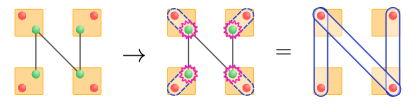
(a)

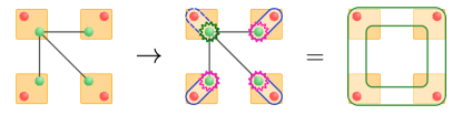
(b)

(c)

Fig. 2: (a) Implametation of a sequence of intermodular control-$Z$ gates. The data qubits (red) are in an arbitrary state, and the memory qubits (green) are initialized in the gate state which corresponds to a graph state. The routine consists in applying a CX gate between the memory and the data qubits followed by a local measurement of the memory qubits. Finally, a correction operation is performed on the data qubits. (b) Implementation of a multiqubit $Z$-rotation with an auxiliary GHZ state. First, a control gate is implemented between the memory and the data qubits. Then all memory qubits except for the central one are measured on the $Z$ basis, and a correction operation is performed on the central memory qubit. Finally, the central memory qubit is measured on the $\theta$ basis $\{e^{-\text{i}\theta X}\left|k\right\rangle\}$, followed by a correction operation on all data qubits.

V.1.1 Diagonal Clifford gates

A gate is called Clifford if it normalizes the Pauli group, i.e., $U$ is Clifford iff $U\,\textbf{P}_{n}\,U^{\dagger}=\textbf{P}_{n}$ where $\textbf{P}_{n}=\left\{e^{\text{i}k\frac{\pi}{2}}X^{\otimes\boldsymbol{i}}Z^{\otimes\boldsymbol{j}}\,|\,\boldsymbol{i},\boldsymbol{j}\in\{0,1\}^{n},k\in\mathbbm{N}\right\}$ is the $n$-Pauli group. Therefore, if $\Lambda$ is Clifford, the outcome gate of routine $T$ is locally unitary (LU) equivalent to $\Lambda$, and it can be converted into it by applying a local correcting operation given by $C^{(\boldsymbol{k})}=\Lambda\,X^{\otimes\boldsymbol{k}}\,\Lambda^{\dagger}X^{\otimes\boldsymbol{k}}\in\textbf{P}_{n}$. Note that in this case, $\Lambda$ can be implemented deterministically by consuming a single copy of its gate state.

Pairwise two-qubit Clifford $Z$-rotation. One example of a diagonal Clifford gate is the control-Z gate, which is given by $\text{CZ}=e^{\text{i}\pi\left|11\right\rangle\!\left\langle 11\right|}\overset{\text{LU}}{\simeq}e^{\text{i}\frac{\pi}{4}ZZ}$. Given a graph $\mathcal{G}$, where a vetice represents a qubit and an edge $(i,j)$ an application of $e^{\text{i}\frac{\pi}{4}ZZ}$ between the $i$th and the $j$th qubits, the corresponding multiqubit gate is given by

$$G=e^{\text{i}\frac{\pi}{4}\sum_{(k,l)\in\mathcal{G}}Z_{k}Z_{l}}.$$

The gate state of $G$ can be directly prepared by evolving the entangling units under the interaction pattern $\mathcal{G}$. Then from $\left|G\right\rangle$, $G$ can be induced by applying $T$ followed by the correction operation $C^{(\boldsymbol{k})}=\prod_{(i,j)\in\mathcal{G}}(Z_{i}Z_{j})^{k_{i}+k_{j}}$, see Fig. 2a.

This is a powerful class of gates as they suffice to implement any intermodular non-Clifford gate, such as multiqubit Z-rotations, i.e., $e^{\text{i}\theta Z^{\otimes n}}\overset{\text{LU}}{\simeq}G^{\dagger}_{1\dots n}\,L^{(\theta)}_{1}\,G_{1\dots n}$, where here $G_{1\dots n}=e^{\text{i}\frac{\pi}{4}Z_{1}(Z_{2}+\cdots+Z_{n})}$ and $L^{(\theta)}=e^{\text{i}(n-1)\frac{\pi}{4}Z}e^{\text{i}\theta X}e^{-\text{i}(n-1)\frac{\pi}{4}Z}$.

Multiqubit Z-rotation. A multiqubit $Z$-rotation $R^{\boldsymbol{j}}\!\left(\theta\right)=e^{\text{i}\theta Z^{\otimes\boldsymbol{j}}}$ is Clifford for $\theta\in\left\{\pm k\pi/4\right\}_{k\in\mathbbm{N}}$, in particular, $R^{\boldsymbol{j}}\!\left(\pm k\pi/4\right)\in\left\{\mathbbm{1},\,Z^{\otimes\boldsymbol{j}},R^{\boldsymbol{j}}\!\left(\pm\pi/4\right)\right\}$. $R^{\boldsymbol{j}}(\pm\pi/4)$ is an entangling gate, and it can be induced from its gate state by applying $T$ followed by the correction operation $C^{(\boldsymbol{k})}=\left(Z^{\otimes\boldsymbol{j}}\right)^{\boldsymbol{k}\cdot\boldsymbol{j}}$ where $\boldsymbol{k}\cdot\boldsymbol{j}=\sum_{i}^{n}k_{i}\,j_{i}$.

V.1.2 Diagonal non-Clifford gates

Non-Clifford gates cannot be deterministically induced from a single copy of its gate state. If the output $\boldsymbol{k}\neq\boldsymbol{0}$ is obtiained, the implemented gate $X^{\otimes\boldsymbol{k}}\Lambda X^{\otimes\boldsymbol{k}}$ is not LU to $\Lambda$. In this case, we need to use other methods. ($i$) One possibility is to decompose $\Lambda$ into a finite sequence of arbitrary multiqubit Z-rotations. As we show later, each of these rotations can be deterministically induced by consuming a Greenberger–Horne–Zeilinger (GHZ) state. ($ii$) Alternatively, one can build a quasi-deterministic protocol by iterating routine $T$ where in each step the target gate is chosen in a heraldic way. We illustrate both methods with specific examples.

Two-qubit Z-rotation. ($i$) An arbitrary two-qubit Z-rotation can be implemented deterministically by consuming a single copy of a two-qubit maximally entangled state, i.e.,

$$(ZZ)_{D_{1}D_{2}}^{(l)}\,Q^{(l)}_{M_{1}D_{1}}\,Z_{M_{1}}^{k}\,T^{(k)}_{M_{2}D_{2}}\left|\text{CZ}\right\rangle_{M_{1}M_{2}}\left|\psi\right\rangle_{D_{1}D_{2}}$$ (4)

$$\mapsto e^{\text{i}\theta ZZ}\left|\psi\right\rangle_{D_{1}D_{2}}$$ ,

where $Q^{(l)}_{ij}=O^{(l)}_{i}e^{\text{i}\theta X}\text{CZ}_{ij}$. Note that this method consumes one ebit of auxiliary entanglement. However, in Ref. [48], it was shown that for small angles, $e^{\text{i}\theta ZZ}$ can be induced by consuming less than one ebit.

($ii$) If we prepare $\left|e^{\text{i}\theta ZZ}\right\rangle$ and apply $T$, we implement

$$T^{(\boldsymbol{k})}_{\textit{MD}}\left|e^{\text{i}\theta ZZ}\right\rangle_{M}\left|\psi\right\rangle_{D}\mapsto e^{\text{i}(-1)^{k_{1}+k_{2}}\theta ZZ}\left|\psi\right\rangle_{D}.$$

Note, with probability $p=1/2$, $e^{\text{i}\theta ZZ}$ is applied and the protocol is over. If not, the rotation is reversed, and we implement $e^{-\text{i}\theta ZZ}$, which can not be locally transformed into the target gate. In case of a failed implementation, we can perform $T$ again with $e^{\text{i}2\theta ZZ}$ as the new target gate. If we succeed the overall gate is given by $e^{\text{i}\theta ZZ}$ and the protocol is over, but in case of failure $e^{-\text{i}3\theta ZZ}$ is implemented. In case of failure, this step is iterated again, being $e^{\text{i}2^{j-1}\theta ZZ}$ the target gate in the $j$th round. As each iteration succeeds with probability $p=1/2$ the protocol provides a quasi-deterministic way of implementing $e^{\text{i}\theta ZZ}$ where the expected number of steps required is given by $\sum_{k=1}^{\infty}k\,2^{-k}=2$. In addition, note that if $\theta=\pi/2^{N}$ where $N\in\mathbbm{N}$, in the $(N-1)$th iteration the target gate is given by $e^{\text{i}\frac{\pi}{4}ZZ}$ which is Clifford and therefore, it can be implemented deterministically. In Appendix. G, we show that for $|\theta|<0.0715\pi$, less than one ebit of entanglement is used on average, and therefore for these values of $\theta$ this second method is more efficient.

Pairwise two-qubit Z-rotations. The same procedure ($ii$) can be used to implement a sequence of non-Clifford pairwise rotations, i.e., $G_{\theta}=e^{\text{i}\sum_{(k,l)\in\mathcal{G}}\theta_{kl}Z_{k}Z_{l}}$. If we prepare its gate state and apply $T$ we implement

$$T^{(\boldsymbol{k})}_{\textit{MD}}\left|G_{\theta}\right\rangle_{M}\left|\psi\right\rangle_{D}\mapsto e^{\text{i}\theta\sum_{(i,j)\in\mathcal{G}}(-1)^{k_{i}+k_{j}}Z_{i}Z_{j}}\left|\psi\right\rangle_{D}.$$

For pairs $(i,j)$ such that $k_{i}\oplus k_{j}=0$ the desired rotation is implemented, while for the other pairs, the rotations are reversed. In the next step, we iterate the procedure with $G^{\prime}_{2\theta}$ as the target gate, where the graph $\mathcal{G}^{\prime}=\mathcal{G}\,\backslash\,\{(i,j)\,|\,k_{i}\oplus k_{j}=0\}$ is given by all edges where the wrong angle was implemented. In this way, $G_{\theta}$ can be quasi-deterministically implemented. See an example in Appendix. E.

Multiqubit Z-rotation. A multiqubit $Z$-rotation $R^{\boldsymbol{j}}(\theta)$ can be implemented with a direct extension of the two methods for the two-qubit $Z$-rotation.

($i$) Equation (4) can be generalized to implement an arbitrary multiqubit $Z$-rotation by consuming a single copy of a GHZ state, i.e.,

$$(Z^{\otimes n})_{D}^{l}\,Q^{(l)}_{M_{1}D_{1}}\,Z^{k_{2}+\dots+k_{n}}_{M_{1}}\,T^{(k_{2},\dots,k_{n})}_{M_{2}D_{2}\dots M_{n}D_{n}}\left|\text{GHZ}\right\rangle_{M}\left|\psi\right\rangle_{D}$$

$$\mapsto e^{\text{i}\theta Z^{\otimes n}}\left|\psi\right\rangle_{D}$$

where $\left|\text{GHZ}\right\rangle=\prod_{j=2}^{n}\text{CZ}_{1j}\left|+\right\rangle^{\otimes n}$, (see Fig. 2b and Appendix. D for details).

$(ii)$ Preparing $\left|R^{\boldsymbol{j}}(\theta)\right\rangle$ and implementing $T$ we obtain an analogous situation to the two-qubit case, i.e,

$$T^{(\boldsymbol{k})}_{\textit{MD}}\left|R^{\boldsymbol{j}}(\theta)\right\rangle_{M}\left|\psi\right\rangle_{D}\mapsto R^{\boldsymbol{j}}\!\left[(-1)^{\boldsymbol{k}\cdot\boldsymbol{j}}\theta\right]\left|\psi\right\rangle_{D},$$

with probability $p=1/2$, we succed and with probability $p=1/2$ the rotation is reversed. Therefore, we can implement $R^{\boldsymbol{j}}(\theta)$ by iterating $T$ in a heraldic way analogously to the two-qubits case.

In this case, the entanglement cost of the two approaches cannot be directly compared. However, in our architecture the second method would be more suitable as the given interaction Hamiltonian allows us to directly establish GHZ states between the modules. Nevertheless, in other settings with a different set-up to interconnect the modules, it could be easier to prepare states of the form $\left|R^{\boldsymbol{j}}(\theta)\right\rangle$ than a GHZ state. In that case, the second method would be more efficient.

Toffoli gate. An $n$-qubit non-Cilfford gate of particular interest is the Toffoli gate, as it is the elementary tool for preparing hypergraph states [49]. The Toffoli gate is given by

$$\text{Toff}\,\overset{\text{LU}}{\simeq}e^{\text{i}\pi\left|\boldsymbol{0}\right\rangle\!\left\langle\boldsymbol{0}\right|}=\prod_{\boldsymbol{j}\in\{0,1\}^{n}}R^{\boldsymbol{j}}\!\left(\pi/2^{n}\right).$$

($i$) The Toffoli gate can be implemented by sequentially performing $R^{\boldsymbol{j}}(\pi/2^{k})$ for every subset of $k$ qubits, which requires to distribute of a GHZ state between each subset of qubits. Because we need to perform $(n-1)$ two-qubit control gates to prepare an $n$-qubit GHZ state, this method requires a total of $1+2^{n-1}(n-2)$ two-qubit intermodular gates. In particular, any diagonal gate $\Lambda$ can be factorized into an arbitrary multi-qubit $Z$-rotation for each subset of qubits (see Appendix. A) and therefore it can be implemented with at most the same number of two-qubit control gates.

($ii$) The implementation following procedure is analogous to the previous examples. We prepare the gate state, apply $T$, and depending on the outcome, for some subsets of qubits the rotation is successfully implemented while for others it is reversed. Then the routine is iterated where the target gate for the $j$th step is given by a rotation of $R^{\boldsymbol{j}}\!\left(2^{j-1}\,\pi/2^{n}\right)$ for all sets $\boldsymbol{j}$ where the implementation failed in the previous steps. Note that in this way, at most $n-1$ steps are required as the target gate for the $(n-1)$th corresponds to a product of Clifford rotations, i.e., $\theta=\pi/4$, and therefore it can be deterministically implemented, see Appendix F for details.

V.2 Non-diagonal gates

An arbitrary $n$-qubit gate can also be stored in the memory units by preparing its Choi state, which is given by

$$\left|\Phi_{U}\right\rangle_{\textit{MM}^{\prime}}=\frac{1}{\sqrt{2^{n}}}\sum_{\boldsymbol{k}\in\{0,1\}^{n}}\left|\boldsymbol{k}\right\rangle_{M}\otimes U\left|\boldsymbol{k}\right\rangle_{M^{\prime}},$$

where $M^{\prime}_{i}$ and $M_{i}$ are two different qubits of the memory of the $i$th module. Note how in this case a $2n$-qubit quantum register where each memory unit hosts two qubits is needed.

Analogously to the diagonal case, given the Choi state of a certain gate $U$, one can find a routine $\widetilde{T}$ that induces $U$ up to a byproduct of local Pauli operators, i.e.,

$$\widetilde{T}^{(\boldsymbol{ij})}_{\textit{MM}^{\prime}\!D}\left|\Phi_{U}\right\rangle_{\textit{MM}^{\prime}}\left|\psi\right\rangle_{D}\mapsto UX^{\otimes\boldsymbol{i}}Z^{\otimes\boldsymbol{j}}\left|\psi\right\rangle_{D},$$ (5)

with probability $p=4^{-n}$ where

$$\widetilde{T}^{(\boldsymbol{ij})}_{\textit{MM}^{\prime}\!D}=O^{(\boldsymbol{i})}_{M}\,O^{(\boldsymbol{j})}_{M^{\prime}}\,\text{H}^{\otimes n}_{M^{\prime}}\,m\text{CX}_{M^{\prime}\to M}\,\text{SWAP}_{M^{\prime}D}.$$

From Eq. (5), it is straightforward to note that Clifford gates can be deterministically induced by performing a local correction operation $C^{(\boldsymbol{i},\boldsymbol{j})}=UZ^{\otimes\boldsymbol{j}}X^{\otimes\boldsymbol{i}}\,U^{\dagger}$. On the other hand, non-Clifford gates can not be corrected with a local gate. Instead one would need to iterate the routine where on the $j$th step the target gate is given by $U^{(j)}=UF^{(j)\dagger}$ where $F^{(j)}$ is the overall gate implemented in the previous steps where the routine failed. In this way, one can construct a (quasi)-deterministic routine for non-Clifford gates.

In this way, given a whole quantum circuit, it always is split into pieces [50], i.e.,

$$U=\prod_{k}\left(U^{(k)}\bigotimes_{i=1}^{n}L^{(k)}\right),$$

where $U^{(k)}$ are intermodular gates that can be induced with a few entangled states, e.g., Clifford gates, arbitrary multiqubit $Z$-rotations or the Toffoli gate, and $L^{(k)}$ are arbitrary modular gates. Once the circuit $U$ is factorized, then intermodular parts $U^{(k)}$ can be run in parallel and stored in the memory units of the modules. Eventually, the whole circuit can be implemented by inducing $U^{(k)}$ while intercalating the modular gates $L^{(k)}$.

VI Summary and conclusions

In this article, we introduced a modular quantum architecture designed to enhance the scalability of quantum information processing. The architecture relies on two independent elements: multipartite entanglement for implementing multiqubit gates and distant-dependent interactions for generating entanglement between modules.

Our scheme introduces how a non-tunable two-body interaction can be used to establish strong interactions between modules without the need to directly tune the interactions and without the need to transmit physical particles or moving systems. On the other hand, our scheme introduces how a quantum circuit can be stored in multipartite entangled states, which allows one to split any quantum circuit into pieces that can be run in parallel. This approach includes and benefits of all the techniques developed for quantum communication allowing for an efficient and scalable quantum computation.

Appendix A Diagonal gates

Note that a projector on a state of the computational basis can be written as

$$\left|\boldsymbol{i}\right\rangle\!\left\langle\boldsymbol{i}\right|=\frac{1}{2^{n}}\sum_{\boldsymbol{j}\in\{0,1\}^{n}}(-1)^{\boldsymbol{i}\cdot\boldsymbol{j}}\,Z^{\otimes\boldsymbol{j}}.$$ (6)

Using Eq. (6), we can factorize any diagonal gate $\Lambda$ into a sequence of multiqubit $Z$-rotations, i.e., given an arbitrary digonal gate where $\left\langle\boldsymbol{i}\right|\Lambda\left|\boldsymbol{i}\right\rangle=e^{\text{i}\alpha_{\boldsymbol{i}}}$ then

$$\Lambda=\sum_{\boldsymbol{i}\in\{0,1\}^{n}}e^{\text{i}\alpha_{\boldsymbol{i}}}\left|\boldsymbol{i}\right\rangle\!\left\langle\boldsymbol{i}\right|=\prod_{\boldsymbol{i}\in\{0,1\}^{n}}e^{\text{i}\alpha_{\boldsymbol{i}}\left|\boldsymbol{i}\right\rangle\!\left\langle\boldsymbol{i}\right|}=\prod_{\boldsymbol{i},\boldsymbol{j}\in\{0,1\}^{n}}e^{\text{i}\alpha_{\boldsymbol{i}}(-1)^{\boldsymbol{i}\cdot\boldsymbol{j}}2^{-n}Z^{\otimes\boldsymbol{j}}}=\prod_{\boldsymbol{j}\in\{0,1\}^{n}}R^{\boldsymbol{j}}(\theta_{\boldsymbol{j}}),$$

where $R^{\boldsymbol{j}}(\theta)=e^{\text{i}\theta Z^{\otimes\boldsymbol{j}}}$ and $\theta_{\boldsymbol{j}}=\sum_{\boldsymbol{i}}(-1)^{\boldsymbol{i}\cdot\boldsymbol{j}}\alpha_{\boldsymbol{i}}/2^{n}$.

Being $\textbf{P}_{n}=\left\{e^{\text{i}\frac{\pi}{2}k}X^{\otimes\boldsymbol{x}}Z^{\otimes\boldsymbol{y}}|k\in\mathbbm{N},\boldsymbol{x},\boldsymbol{y}\in\{0,1\}^{n}\right\}$ the $n$-Pauli group, $\Lambda$ is said to be Clifford iff

$$\begin{gathered}\Lambda^{\dagger}\,X^{\otimes\boldsymbol{k}}\,Z^{\otimes\boldsymbol{l}}\,\Lambda\in\textbf{P}_{n}\;\;\forall\,\boldsymbol{k},\boldsymbol{l}\\ \Leftrightarrow\;\Lambda^{\dagger}\,X^{\otimes\boldsymbol{k}}\,\Lambda\,X^{\otimes\boldsymbol{k}}=\Lambda^{\dagger}\prod_{\boldsymbol{j}}R^{\boldsymbol{j}}\!\left[(-1)^{\boldsymbol{j}\cdot\boldsymbol{k}}\theta_{\boldsymbol{j}}\right]=\prod_{\boldsymbol{j}}R^{\boldsymbol{j}}\!\left(\omega_{\boldsymbol{jk}}\right)=\prod_{\boldsymbol{j}}\left[\cos(\omega_{\boldsymbol{jk}})\,\mathbbm{1}+\text{i}\sin(\omega_{\boldsymbol{jk}})\,Z^{\otimes\boldsymbol{j}}\right]\in\textbf{P}_{n}\;\;\forall\,\boldsymbol{k}\end{gathered}$$

where $\omega_{\boldsymbol{ij}}=\left[(-1)^{\boldsymbol{i}\cdot\boldsymbol{j}}-1\right]\theta_{\boldsymbol{j}}\in\{0,2\theta_{\boldsymbol{j}}\}$. Therefore, $\Lambda$ is Clifford iff it can be factorized into multiqubit rotations of the from $\theta_{\boldsymbol{j}}\in\left\{\pm k\pi/4\right\}_{k\in\mathbbm{N}}\;\forall\,\boldsymbol{j}$.

Appendix B Induction of Z-diagonal gates

Given an arbitrary $n$-qubit diagonal gate

$$\Lambda=\sum_{\boldsymbol{i}\in\{0,1\}^{n}}e^{\text{i}\alpha_{\boldsymbol{i}}}\left|\boldsymbol{i}\right\rangle\!\left\langle\boldsymbol{i}\right|,$$ (7)

consider its gate state $\left|\Lambda\right\rangle$ and an arbitrary $n$-qubit state

$$\left|\psi\right\rangle_{D}=\sum_{\boldsymbol{j}}\psi_{\boldsymbol{j}}\left|\boldsymbol{j}\right\rangle_{D}.$$ (8)

If we apply a multilateral control-$X$ between the two-state and measure the $M$ qubits, i.e.,

$$T_{\textit{MD}}^{(\boldsymbol{k})}=\left(O^{(k_{i})}_{M_{1}}\,\text{CX}_{D_{i}M_{i}}\right),$$

we implement $\Lambda$ up to a byproduct of Pauli $X$ gates to the $D$ system, i.e.,

$$T_{\textit{MD}}^{(\boldsymbol{k})}\,\left|\Lambda\right\rangle_{M}\left|\psi\right\rangle_{D}=\frac{1}{\sqrt{2^{n}}}\,T_{\textit{MD}}^{(\boldsymbol{k})}\sum_{\boldsymbol{i},\boldsymbol{j}}e^{\text{i}\alpha_{\boldsymbol{j}}}\,\psi_{\boldsymbol{j}}\left|\boldsymbol{j}\right\rangle_{M}\left|\boldsymbol{i}\right\rangle_{D}=\frac{1}{\sqrt{2^{n}}}\,O_{M}^{(\boldsymbol{k})}\sum_{\boldsymbol{i},\boldsymbol{j}}e^{\text{i}\alpha_{\boldsymbol{j}}}\psi_{\boldsymbol{i}}\left|\boldsymbol{j}\oplus\boldsymbol{i}\right\rangle_{M}\left|\boldsymbol{i}\right\rangle_{D}$$

$$\mapsto\sum_{\boldsymbol{i}}e^{\text{i}\alpha_{\boldsymbol{i}\oplus\boldsymbol{k}}}\,\psi_{\boldsymbol{i}}\left|\boldsymbol{i}\right\rangle_{D}=X^{\otimes\boldsymbol{k}}\sum_{\boldsymbol{i}}e^{\text{i}\alpha_{\boldsymbol{i}}}\,\psi_{\boldsymbol{i}\oplus\boldsymbol{k}}\left|\boldsymbol{i}\right\rangle_{D}=X^{\otimes\boldsymbol{k}}\,\Lambda\,X^{\otimes\boldsymbol{k}}\left|\psi\right\rangle_{D}$$ ,

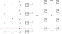
(a) $T^{(\boldsymbol{n})}$

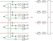
(b) $\widetilde{T}^{(\boldsymbol{n},\boldsymbol{m})}$

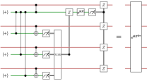
(c) $(Z^{\otimes n})^{l}_{D}\,Q_{M_{1}D_{1}}\,Z_{M_{1}}^{k_{2}+\cdots+k_{1}}\,T^{(k_{2},\dots,k_{n})}_{M_{2}D_{2}\dots M_{n}D_{n}}$

Fig. 4: (a) Probabilistic induction of a multiqubit gate $U$. (b) Probabilistic induction of a diagonal gate $\Lambda$. (c) Deterministic implementation of an arbitrary multi-Z-rotation with an auxiliary GHZ state.

see Fig. 4a for the circuit representation. Note the probability of obtaining outcome $O^{(\boldsymbol{k})}$ is independent of $\boldsymbol{k}$, i.e.,

$$p(\boldsymbol{k})=\sum_{\boldsymbol{l}}\left|\left\langle\boldsymbol{k},\boldsymbol{l}\right|m\text{CX}\left|\Lambda,\psi\right\rangle\right|^{2}=\sum_{\boldsymbol{l}}\Big{|}\left\langle\boldsymbol{k},\boldsymbol{l}\right|\frac{1}{\sqrt{2^{n}}}\,\sum_{\boldsymbol{i},\boldsymbol{j}}e^{\text{i}\alpha_{\boldsymbol{j}}}\,\psi_{\boldsymbol{i}}\left|\boldsymbol{j}\oplus\boldsymbol{i},\boldsymbol{i}\right\rangle\Big{|}^{2}=\frac{1}{2^{n}}\sum_{\boldsymbol{l}}\left|e^{\text{i}\alpha_{\boldsymbol{k}\oplus\boldsymbol{l}}}\,\psi_{\boldsymbol{l}}\right|^{2}=\frac{1}{2^{n}}\sum_{\boldsymbol{l}}\left|\psi_{\boldsymbol{l}}\right|^{2}=\frac{1}{2^{n}}.$$

Appendix C Induction of arbitrary gates

Conisder an arbitrary $n$-qubit gate,

$$U=\sum_{\boldsymbol{l},\boldsymbol{k}}u_{\boldsymbol{lk}}\left|\boldsymbol{l}\right\rangle\!\left\langle\boldsymbol{k}\right|,$$ (9)

and its Choi state

$$\left|\Phi_{U}\right\rangle_{\textit{MM}^{\prime}}=\frac{1}{\sqrt{2^{n}}}\sum_{\boldsymbol{k}}\left|\boldsymbol{k}\right\rangle_{M}\otimes U\left|\boldsymbol{k}\right\rangle_{M^{\prime}}=\frac{1}{\sqrt{2^{n}}}\sum_{\boldsymbol{k},\boldsymbol{l}}u_{\boldsymbol{lk}}\left|\boldsymbol{k}\right\rangle_{M}\otimes\left|\boldsymbol{l}\right\rangle_{M^{\prime}}.$$ (10)

Given an arbitrary $n$-qubit state $\left|\psi\right\rangle_{D}$, we can induce $U$ up to a random byproduct of Pauli gates by applying a local routine $\widetilde{T}$ that consists in applying a multilateral control-$X$ gate between $D$ and $M$ followed by a projective measurement on the Choi state. In particular with probability $p=4^{-n}$ we implement

$$\widetilde{T}^{(\boldsymbol{nm})}_{\textit{MM}^{\prime}\!D}=O^{(\boldsymbol{n})}_{M}\,O^{(\boldsymbol{m})}_{M^{\prime}}\,\text{H}^{\otimes n}_{M^{\prime}}\,m\text{CX}_{M^{\prime}\to M}\,\text{SWAP}_{M^{\prime}D}.$$

Routine $\widetilde{T}$ induces $U$ up to a byproduct of local Pauli gates, i.e.,

$$\widetilde{T}^{(\boldsymbol{rs})}_{\textit{MM}^{\prime}\!D}\left|\Phi_{U}\right\rangle_{\textit{MM}^{\prime}}\left|\psi\right\rangle_{D}$$

$$=\frac{1}{\sqrt{2^{n}}}\,O^{(\boldsymbol{r})}_{M}\,O^{(\boldsymbol{s})}_{M^{\prime}}\,\text{H}^{\otimes n}_{M^{\prime}}\,m\text{CX}_{M^{\prime}\to M}\sum_{\boldsymbol{k},\boldsymbol{l},\boldsymbol{j}}\psi_{\boldsymbol{j}}\,u_{\boldsymbol{lk}}\left|\boldsymbol{k},\boldsymbol{j}\right\rangle_{\textit{MM}^{\prime}}\left|\boldsymbol{l}\right\rangle_{D}$$

$$=\frac{1}{\sqrt{2^{n}}}\,O^{(\boldsymbol{r})}_{M}\,O^{(\boldsymbol{s})}_{M^{\prime}}\,\text{H}^{\otimes n}_{M^{\prime}}\,\sum_{\boldsymbol{k},\boldsymbol{l},\boldsymbol{j}}\psi_{\boldsymbol{j}}\,u_{\boldsymbol{lk}}\left|\boldsymbol{k}\oplus\boldsymbol{j},\boldsymbol{j}\right\rangle_{\textit{MM}^{\prime}}\left|\boldsymbol{l}\right\rangle_{D}$$

$$=\frac{1}{\sqrt{2^{n}}}\,O^{(\boldsymbol{r})}_{M}\,O^{(\boldsymbol{s})}_{M^{\prime}}\,\sum_{\boldsymbol{k},\boldsymbol{l},\boldsymbol{i},\boldsymbol{j}}(-1)^{\boldsymbol{i}\cdot\boldsymbol{\boldsymbol{j}}}\,\psi_{\boldsymbol{j}}\,u_{\boldsymbol{lk}}\left|\boldsymbol{k}\oplus\boldsymbol{j},\boldsymbol{i}\right\rangle_{\textit{MM}^{\prime}}\left|\boldsymbol{l}\right\rangle_{D}$$

$$\mapsto\sum_{\boldsymbol{k},\boldsymbol{l}}(-1)^{\boldsymbol{s}\cdot(\boldsymbol{r}\oplus\boldsymbol{k})}\,\psi_{\boldsymbol{r}\oplus\boldsymbol{k}}\,u_{\boldsymbol{lk}}\left|\boldsymbol{l}\right\rangle_{D}$$

$$=UX^{\otimes\boldsymbol{r}}Z^{\otimes\boldsymbol{s}}\left|\psi\right\rangle_{D}$$ .

where we have used that $H^{\otimes n}=\sum_{\boldsymbol{i},\boldsymbol{j}}(-1)^{\boldsymbol{i}\cdot\boldsymbol{j}}\left|\boldsymbol{i}\right\rangle\!\left\langle\boldsymbol{j}\right|$. See in Fig. 4b the circuit representation.

Appendix D Multi-qubit Z-rotation

In this section, we show in detail how a GHZ can be used to implement a multiqubit $Z$-rotation, shown in Sec. V.1.2. The protocol consists of applying

$$Z_{M_{1}}^{k_{2}+\cdots+k_{n}}\,T^{(k_{2},\dots,k_{n})}_{M_{2}D_{2}\dots M_{n}D_{n}}=Z_{M_{1}}^{k_{2}+\cdots+k_{n}}\bigotimes_{i=2}^{n}\left(O^{(k_{i})}\text{CX}_{D_{i}\to M_{1}}\right),$$

followed by

$$(Z^{\otimes n})^{l}_{D}\,Q_{M_{1}D_{1}}=(Z^{\otimes n})^{l}_{D}\,O^{(l)}_{M_{1}}\,e^{\text{i}\theta X_{M_{1}}}\text{CZ}_{M_{1}D_{1}},$$

where $O^{(k)}=\left|k\right\rangle\!\left\langle k\right|$ to an arbitrary $n$-qubit gate $\left|\psi\right\rangle_{D}$ and a $\left|\text{GHZ}\right\rangle_{M}=\prod_{i=2}^{n}\text{CZ}_{1,i}\left|+\right\rangle^{\otimes n}$, i.e.,

$$(Z^{\otimes n})^{l}_{D}\,Q_{M_{1}D_{1}}\,Z_{M_{1}}^{k_{2}+\cdots+k_{n}}\,T^{(k_{2},\dots,k_{n})}_{M_{2}D_{2}\dots M_{n}D_{n}}\left|\text{GHZ}\right\rangle_{M}\left|\psi\right\rangle_{D}$$

$$=\frac{1}{2^{n/2}}\,(Z^{\otimes n})^{l}_{D}\,Q_{M_{1}D_{1}}\,Z_{M_{1}}^{k_{2}+\cdots+k_{n}}\,T^{(k_{2},\dots,k_{n})}_{M_{2}D_{2}\dots M_{n}D_{n}}\sum_{\boldsymbol{i},\boldsymbol{j}}\psi_{\boldsymbol{i}}\left(-1\right)^{j_{1}(j_{2}+\dots+j_{n})}\left|\boldsymbol{j}\right\rangle_{M}\left|\boldsymbol{i}\right\rangle_{D}$$

$$\mapsto\frac{1}{\sqrt{2}}(Z^{\otimes n})^{l}_{D}\,Q_{M_{1}D_{1}}\,Z_{M_{1}}^{k_{2}+\dots+k_{n}}\sum_{\boldsymbol{i},j_{1}}\psi_{\boldsymbol{i}}\left(-1\right)^{j_{1}(i_{2}+k_{2}+\dots+i_{n}+k_{n})}\left|j_{1}\right\rangle_{M_{1}}\left|\boldsymbol{i}\right\rangle_{D}$$

$$=\frac{1}{\sqrt{2}}(Z^{\otimes n})^{l}_{D}\,Q_{M_{1}D_{1}}\,\sum_{\boldsymbol{i},j_{1}}\psi_{\boldsymbol{i}}\left(-1\right)^{j_{1}(i_{2}+\dots+i_{n})}\left|j_{1}\right\rangle_{M_{1}}\left|\boldsymbol{i}\right\rangle_{D}$$

$$\mapsto(Z^{\otimes n})^{l}_{D}\,\sum_{\boldsymbol{i}}\psi_{\boldsymbol{i}}\left(-1\right)^{l\sum_{k}i_{k}}e^{\text{i}(-1)^{\sum_{k}i_{k}}\theta}\left|\boldsymbol{i}\right\rangle_{D}$$

$$=\sum_{\boldsymbol{i}}\psi_{\boldsymbol{i}}\,e^{\text{i}(-1)^{\sum_{k}i_{k}}\theta}\left|\boldsymbol{i}\right\rangle_{D}$$

$$=e^{\text{i}\theta Z^{\otimes n}}\left|\psi\right\rangle_{D}$$ ,

see Fig. 4c for the circuit representation.

Appendix E Paiwise two-quit Z-rotations: Particular example

Conisder four modules and the target intermodular gate

$$G_{\pi/16}=e^{\text{i}\frac{\pi}{16}(Z_{1}Z_{3}+Z_{1}Z_{4}+Z_{2}Z_{4}+Z_{3}Z_{4})}.$$

Such a gate is non-Clifford and therefore, we need to sequentially apply routine $T$ until we succeed.

1st step. We prepare its gate state and apply $T$. We assume outomce $\boldsymbol{k}_{1}=(0,1,0,1)$ is obtained. Then the implemented gate is given by

$$X_{2}\,X_{4}\,G_{\pi/16}\,X_{2}\,X_{4}=e^{\text{i}\frac{\pi}{16}(Z_{1}Z_{3}-Z_{1}Z_{4}+Z_{2}Z_{4}-Z_{3}Z_{4})}.$$

Note the rotation is successfully implemented for pairs (1,3) and (2,4), while for pairs (1,4) and (3,4) it is reversed.

2nd step. We want to correct the rotation for the pairs where we failed in the last step. Therefore, in this step, our target gate is given by

$$G^{\prime}_{\pi/8}=e^{\text{i}\frac{\pi}{8}(Z_{1}Z_{4}+Z_{3}Z_{4})}$$

We prepare its gate state and apply $T$. If we assume outcome $\boldsymbol{k}_{2}=(0,\varnothing,1,1)$ is obtained, the implemented gate is given by

$$X_{3}\,X_{4}\,G^{\prime}_{\pi/8}\,X_{3}\,X_{4}=e^{\text{i}\frac{\pi}{8}(-Z_{1}Z_{4}+Z_{3}Z_{4})},$$

and the overall gate implemented is given by

$$X_{3}\,X_{4}\,G^{\prime}_{\pi/8}\,X_{3}\,X_{4}\,X_{2}\,X_{4}\,G_{\pi/16}\,X_{2}\,X_{4}=e^{\text{i}\frac{3\pi}{8}Z_{1}Z_{4}}e^{\text{i}\frac{\pi}{16}(Z_{1}Z_{3}+Z_{2}Z_{4}+Z_{3}Z_{4})}.$$

Note that after this second step, our initial target rotation is successfully implemented for pairs (1,3), (2,4) and (3,4), while for pair (1,4) we failed in both steps.

3rt step. We need to implement

$$G^{\prime\prime}_{\pi/4}=e^{\text{i}\frac{\pi}{4}Z_{1}Z_{4}}$$

Note that $G^{\prime\prime}_{\pi/4}$ is Clifford, and therefore it can be deterministically implemented by performing a local correction operation, i.e., if outcome $\boldsymbol{k}_{3}=(l,\varnothing,\varnothing,k)$ is obtained then the correction operation is given by $(Z_{1}Z_{4})^{l+k}$, and

$$(Z_{1}\,Z_{4})^{l+k}\,X_{1}^{l}\,X_{4}^{k}\,G^{\prime\prime}_{\pi/4}\,X_{1}^{l}\,X_{4}^{k}=G^{\prime\prime}_{\pi/4}.$$

Therefore, after the third step, the overall gate is given by

$$G^{\prime\prime}_{\pi/4}\,e^{\text{i}\frac{3\pi}{8}Z_{1}Z_{4}}e^{\text{i}\frac{\pi}{16}(Z_{1}Z_{3}+Z_{2}Z_{4}+Z_{3}Z_{4})}=G_{\pi/16}.$$

and the implementation is over. See Fig. 3.

(1)

(2)

(3)

(4)

(5)

(6)

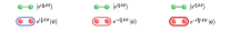
(7)

Fig. 3: Implementation of $G_{\pi/16}$ where $\mathcal{G}=\{V=\{1,2,3,4\},E=\{(1,3),(1,4),(2,4),(3.4)\}\}$, with routine $T$. First, we prepare the gate state $\left|G_{\pi/16}\right\rangle$ and apply $T$. If we obtain output $\boldsymbol{k}_{1}=(0,1,0,1)$, the gate is only implemented correctly between qubits (1,3) and (2,4). In a second step, we prepare the gate state $\left|G^{\prime}_{\pi/8}\right\rangle$ where $\mathcal{G}^{\prime}=\{V=\{1,2,4\},E=\{(1,4),(3.4)\}\}$ and we apply $T$. If in the second step, we obtain $\boldsymbol{k}_{2}=(0,1,1)$ we succeed in edge (3,4). In the last step we prepare the gate state $\left|G^{\prime\prime}_{\pi/4}\right\rangle$ where $\mathcal{G}^{\prime\prime}=\{V=\{1,4\},E=\{(1,4)\}\}$ and we apply $T$. Because $G^{\prime\prime}_{\pi/4}$ is Clifford we succeed for all outcomes. After the third state, the overall gate implemented is given by $G_{\pi/4}$.

Appendix F Inducing the Toffoli gate with routine T

We show in detail how to induce the Toffoli gate by applying routine $T$. The Toffoloi gate is LU equivalent to

$$F=e^{\text{i}\pi\left|\boldsymbol{0}\right\rangle\!\left\langle\boldsymbol{0}\right|}.$$

1st step: We try to induce $F$ by preparing $\left|F\right\rangle_{M}$ and applying $T$, i.e.,

$$T_{\textit{MD}}^{(\boldsymbol{k}_{1})}\!:\,\left|F\right\rangle_{M}\left|\psi_{0}\right\rangle_{D}\;\mapsto\;\left|\psi_{1}\right\rangle_{D}=W_{1}\left|\psi_{0}\right\rangle_{D}$$

where $W_{1}=X^{\otimes\boldsymbol{k}_{1}}FX^{\otimes\boldsymbol{k}_{1}}=e^{\text{i}\pi\left|\boldsymbol{k}_{1}\right\rangle\!\left\langle\boldsymbol{k}_{1}\right|}$. With probability $p_{1}=2^{-n}$, we obtain $\boldsymbol{k}_{1}=\boldsymbol{0}$ and $W_{1}=F$ is successfully implemented, otherwise, we fail and proceed with step 2.

2nd step: We try to undue $W_{1}$ and implement $F$, so we prepare $\left|FW_{1}\right\rangle$ (becouse $W_{1}^{\dagger}=W_{1}$) and apply $T$, i.e.,

$$T_{\textit{MD}}^{(\boldsymbol{k}_{2})}\!:\,\left|W_{1}F\right\rangle_{M}\left|\psi_{1}\right\rangle_{D}\;\mapsto\;\left|\psi_{2}\right\rangle_{D}=W_{2}\left|\psi_{1}\right\rangle_{D}=W_{2}\,W_{1}\left|\psi_{0}\right\rangle_{D},$$

$W_{2}=X^{\otimes\boldsymbol{k}_{2}}W_{1}FX^{\otimes\boldsymbol{k}_{2}}=e^{\text{i}\pi\left(\left|\boldsymbol{k}_{1}\oplus\boldsymbol{k_{2}}\right\rangle\!\left\langle\boldsymbol{k}_{1}\oplus\boldsymbol{k_{2}}\right|+\left|\boldsymbol{k}_{2}\right\rangle\!\left\langle\boldsymbol{k}_{2}\right|\right)}$, and therefore the gate implemented after the 2nd step is given by

$$W_{2}\,W_{1}=e^{\text{i}\pi\left(\left|\boldsymbol{k}_{1}\right\rangle\!\left\langle\boldsymbol{k}_{1}\right|+\left|\boldsymbol{k}_{2}\right\rangle\!\left\langle\boldsymbol{k}_{2}\right|+\left|\boldsymbol{k}_{1}\oplus\boldsymbol{k_{2}}\right\rangle\!\left\langle\boldsymbol{k}_{1}\oplus\boldsymbol{k_{2}}\right|\right)}.$$

Note that $W_{2}\,W_{1}=F$ for $\boldsymbol{k}_{2}\in\{\boldsymbol{k}_{1},\boldsymbol{0}\}$, and therefore, the success probability is $p_{2}=2\cdot 2^{-n}$. In case of failure, we go with step three.

3rd step: We try to undue $W_{2}W_{1}$ and implement $F$, so we prepare $\left|FW_{1}W_{2}\right\rangle$ (becouse $W_{2}^{\dagger}=W_{2}$) and apply $T$, i.e.,

$$T_{\textit{MD}}^{(\boldsymbol{k}_{3})}\!:\,\left|W_{2}W_{1}F\right\rangle_{M}\left|\psi_{2}\right\rangle_{D}\;\mapsto\;\left|\psi_{3}\right\rangle_{D}=W_{3}\left|\psi_{2}\right\rangle_{D}=W_{3}\,W_{2}\,W_{1}\left|\psi_{0}\right\rangle_{D},$$

where

$$W_{3}=X^{\otimes\boldsymbol{k}_{3}}F\,W_{1}\,W_{2}\,X^{\otimes\boldsymbol{k}_{3}},$$

and hence the gate implemented after the step 3 is given by

$$W_{3}\,W_{2}\,W_{3}=F\prod_{\boldsymbol{k}\in\Xi_{3}}e^{\text{i}\pi\left|\boldsymbol{k}\right\rangle\!\left\langle\boldsymbol{k}\right|},$$

where $\Xi_{3}=\{\boldsymbol{0},\boldsymbol{k}_{1},\boldsymbol{k}_{2},\boldsymbol{k}_{3},\boldsymbol{k}_{1}\oplus\boldsymbol{k}_{2},\boldsymbol{k}_{1}\oplus\boldsymbol{k}_{3},\boldsymbol{k}_{2}\oplus\boldsymbol{k}_{3},\boldsymbol{k}_{1}\oplus\boldsymbol{k}_{2}\oplus\boldsymbol{k}_{3}\}$. Note that $W_{3}W_{2}W_{1}=F$ for $\boldsymbol{k}_{3}\in\Xi_{2}=\{\boldsymbol{k}_{1},\boldsymbol{k}_{2},\boldsymbol{k}_{1}\oplus\boldsymbol{k}_{2}\}$, and therefore, the success probability is $p_{3}=4\cdot 2^{-n}$. In case of failure, we go with the 4th step.

jth step: We try to undue $W_{j-1}\cdots W_{2}\,W_{1}$ and induce $F$, so we prepare $\left|FW_{1}W_{2}\cdots W_{j-1}\right\rangle$ (becouse $W_{j-1}^{\dagger}=W_{j-1}$) and apply $T$, i.e.,

$$T_{\textit{MD}}^{(\boldsymbol{k}_{j})}\!:\,\left|W_{j-1}\cdots W_{2}W_{1}F\right\rangle_{M}\left|\psi_{j-1}\right\rangle_{D}\;\mapsto\;\left|\psi_{j}\right\rangle_{D}=W_{j}\left|\psi_{j-1}\right\rangle_{D}=W_{j}\cdots W_{2}\,W_{1}\left|\psi_{0}\right\rangle_{D},$$

where

$$W_{j}=X^{\boldsymbol{k}_{j}}\,F\,W_{j-1}\cdots W_{2}\,W_{1}\,X^{\boldsymbol{k}_{j}}$$

and the accumulated gate

$$W_{j}\cdots W_{2}\,W_{1}=F\prod_{\boldsymbol{k}\in\Xi_{j}}e^{\text{i}\pi\left|\boldsymbol{k}\right\rangle\!\left\langle\boldsymbol{k}\right|},$$

where $\Xi_{j}=\langle\{\boldsymbol{k}_{1},\dots\boldsymbol{k}_{j}\}\rangle_{\oplus}$, and $\langle\{\bullet\}\rangle_{\oplus}$ denotes the set generated by $\{\bullet\}$ with the operation vector sum mod(2) “$\oplus$”. Note that $\Xi_{k}$ contains $|\Xi_{j}|=2^{j}$ elements, and we succeed if $\boldsymbol{k}_{j}\in\Xi_{j-1}$. Therefore, the success probability is given by $p_{j}=|\Xi_{j-1}|\,2^{-n}=2^{j-1}\,2^{-n}$. This means the success probability is doubled in each step. Following the equation $p_{j}=2^{j-1}\,2^{-n}$, one would expect that $n+1$ steps are required to achieve a deterministic implementation. However, at the $(n-1)$th step the gate

$$W_{n-1}\cdots W_{1}=F\prod_{\boldsymbol{k}\in\Xi_{n-1}}e^{\text{i}\pi\left|\boldsymbol{k}\right\rangle\!\left\langle\boldsymbol{k}\right|},$$

is Clifford as we have shown in Sec. V.1.2, and in case we fail we can correct it with a local operation.

Appendix G Entanglement cost

Given a bipartite state $\left|\psi\right\rangle_{AB}$, its entropy of entanglement is given by

$$E=-\text{tr}\left(\rho_{A}\log_{2}\rho_{A}\right)$$

where $\rho_{A}=\text{tr}_{B}\left|\psi\right\rangle\!\left\langle\psi\right|$. The entanglement in the gate state of a two-qubit gate rotation $e^{\text{i}\theta ZZ}$ is given by

$$E\!\left(\theta\right)=-x\log_{2}(x)-(1-x)\log_{2}(1-x)$$

where $x=\cos^{2}(\theta)$.

If we compute the entanglement cost of implementation of a two-qubit $Z$-rotation of the two methods shown in Sec. V.1.2, we obtain that with the deterministic approach a Bell state is always destroyed and therefore it has a fixed cost of one ebit. On the other hand, sequentially applying routine $T$, we consume $E(2^{k-1}\theta)$ ebits in the $j$th iteration, and therefore the expected value ebits is given by

$$\left\langle E\,\right\rangle=\sum_{k=1}^{\infty}\left(\frac{1}{2}\right)^{k-1}E\!\left(2^{k-1}\theta\right).$$

Note that $\left\langle E\,\right\rangle<1$ for $|\theta|<0.2245$, which means for these angles it is more efficient to induce $e^{\text{i}\theta ZZ}$ with the $T$ gate. Otherwise, we would use a bell state.