Causal-Consistent Reversible Debugging:
Improving CauDEr

Abstract

Causal-consistent reversible debugging allows one to explore concurrent computations back and forth in order to locate the source of an error. In this setting, backward steps can be chosen freely as long as they are causal consistent, i.e., as long as all the actions that depend on the action we want to undo have been already undone. Here, we consider a framework for causal-consistent reversible debugging in the functional and concurrent language Erlang. This framework considered programs translated to an intermediate representation, called Core Erlang. Although using such an intermediate representation simplified both the formal definitions and their implementation in a debugging tool, the choice of Core Erlang also complicated the use of the debugger. In this paper, we extend the framework in order to deal with source Erlang programs, also including some features that were not considered before. Moreover, we integrate the two existing approaches (user-driven debugging and replay debugging) into a single, more general framework, and develop a new version of the debugging tool CauDEr including all the mentioned extensions as well as a renovated user interface.
Published as González-Abril, J.J. and Vidal, G. (2021). Causal-Consistent Reversible Debugging: Improving CauDEr. In: Morales, J.F. and Orchard, D.A. (eds) Practical Aspects of Declarative Languages. PADL 2021. Lecture Notes in Computer Science, vol 12548. Springer.
The final authenticated publication is available at https://doi.org/10.1007/978-3-030-67438-0_9

1 Introduction

Reversible debugging is a well established technique [3, 17] which advocates that, in order to find the location of an error, it is often more natural to explore a computation backwards from the observable misbehavior. Therefore, reversible debuggers allow one to explore a computation back and forth. There are already a number of software debuggers that follow this idea (e.g., Undo [16]). Typically, one can undo the steps of a computation in exactly the inverse order of the original forward computation. However, in the context of a concurrent language like Erlang, reversible debugging becomes much more complex. On the one hand, in these languages, there is no clear (total) order for the actions of the concurrent processes, since the semantics is often nondeterministic. On the other hand, one is typically interested in a particular process, e.g., the one that exhibited a misbehavior. Thus, undoing the steps of all processes in the very same order of the forward computation is very inconvenient, since we had to go through many actions that are completely unrelated to the process of interest.

Recently, causal-consistent reversible debugging [2] has been introduced in order to overcome these problems. In this setting, concurrent actions can be undone freely as long as they are causal-consistent, i.e., no action is undone until all the actions that depend on this one have been already undone. For instance, one cannot undo the spawning of a process until all the actions of this process have been undone.

A reversible semantics for (Core) Erlang was first introduced in [12] and, then, extended and improved in [8]. A causal-consistent reversible debugger, CauDEr, that follows these ideas was then presented in [7]. In the original approach, both the forward and the backward computations were driven by the user (i.e., the user selects the process of interest as well as the message to be received when there are several possibilities), so we refer to this approach as user-driven debugging. However, when a computation fails, it is often very difficult, even impossible, to replicate the same computation in the debugger. This is a well-known problem in the debugging of concurrent programs. Therefore, [10] introduces a novel approach, called replay debugging, that is based on a light program instrumentation so that the execution of the instrumented program produces an associated log. This log can then be used for the debugger to replay the same computation or a causally equivalent one (i.e., one that at least respects the same order between dependent actions).

Unfortunately, all these works consider the intermediate language Core Erlang [1]. Dealing with (a subset of) Core Erlang made the theoretical developments easier (without loss of generality, since programs are automatically transformed from source Erlang to Core Erlang during the compilation process). The reversible debugger CauDEr considers Core Erlang too, which greatly simplified the implementation task. Unfortunately, as a result, the debugger is rather difficult to use since the programmer is often not familiar with the Core Erlang representation of her program. Compare, for instance, the following Erlang code defining the factorial function:

  fact(0)          -> 1;
  fact(N) when N>0 -> N * fact(N-1).

and the corresponding representation in Core Erlang:

’fact’/1 =
  fun (_0) ->
    case _0 of
      <0> when ’true’ -> 1
      <N> when call ’erlang’:’>’(N, 0) ->
          let <_1> = call ’erlang’:’-’(N, 1)
          in let <_2> = apply ’fact’/1(_1)
          in call ’erlang’:’*’(N, _2)
      <_3> when ’true’ ->
          primop ’match_fail’({’function_clause’,_3})
    end
end

On the other hand, while Erlang remains relatively stable, the Core Erlang specification changes (often undocumented) with some releases of the Erlang/OTP compiler, which makes maintaining the debugger quite a difficult task.

In this paper, we extend the causal-consistent approach to reversible debugging of Erlang in order to deal with (a significant subset of) the source language. The main contributions are the following:

• We redefine both the standard and the reversible semantics in order to deal with source Erlang expressions.

• Moreover, we integrate the two previous approaches, the user-driven reversible debugger of [8] and the replay debugger of [10], intro a single, more general framework.

• Finally, we have implemented a new version of the CauDEr reversible debugger [7] which implements the above contributions, also redesigning the user interface.

Missing details can be found in the appendix.

2 The Source Language

In this section, we informally introduce the syntax and semantics of the considered language, a significant subset of Erlang. A complete, more formal definition can be found in the appendix. We also discuss the main differences with previous work that considered Core Erlang instead.

Erlang is a typical higher-order, eager functional language extended with some additional features for message-passing concurrency. Let us first consider the sequential component of the language, which includes the following elements:

• Variables, denoted with identifiers that start with an uppercase letter.

• Atoms, denoted with identifiers that start with a lowercase letter. Atoms are used, e.g., to denote constants and function names.

• Data constructors. Erlang only considers lists (using Prolog notation, i.e., $[e_{1}|e_{2}]$ denotes a list with first element $e_{1}$ and tail $e_{2}$) and tuples, denoted by an expression of the form $\{e_{1},\ldots,e_{n}\}$, where $e_{1},\ldots,e_{n}$ are expressions, $n\geq 0$. However, Erlang does not allow user-defined constructors as in, e.g., Haskell.

• Values, which are built from literals (e.g., numbers), atoms and data constructors.

• Patterns, which are similar to values but might also include variables.

• Expressions. Besides variables, values and patterns, we consider the following types of expressions:

  • Sequences of the form $e_{1},\ldots,e_{n}$ where $e_{i}$ is a single expression (i.e., it cannot be a sequence), $i=1,\ldots,n$. Evaluation proceeds from left to right: first, we evaluate $e_{1}$ to some value $v_{1}$ thus producing $v_{1},e_{2},\ldots,e_{n}$. If $n>1$, the sequence is then reduced to $e_{2},\ldots,e_{n}$, and so forth. Therefore, sequences are eventually evaluated to a (single) value. The use of sequences of expressions in the right-hand sides of functions is a distinctive feature of Erlang. In the following, we assume that all expressions are single expressions except otherwise stated.

  • Pattern matching equations of the form $p=e$, where $p$ is a pattern and $e$ is an expression. Here, we evaluate $e$ to a value $v$ and, then, try to find a substitution $\sigma$ such that $p\sigma=v$. If so, the equation is reduced to $v$ and $\sigma$ is applied to the complete expression. E.g., the expression “$\tt\{X,Y\}=\{ok,40+2\},X$” is reduced to “$\tt\{ok,42\},ok$” and, then, to $\tt ok$.

  • Case expressions like $\mathsf{case}~{}e~{}\mathsf{of}~{}cl_{1};\ldots;cl_{n}~{}\mathsf{end}$, where each clause $cl_{i}$ has the form “$p_{i}~{}[\mathsf{when}~{}g_{i}]\to e_{i}$” with $p_{i}$ a pattern, $g_{i}$ a guard and $e_{i}$ an expression (possibly a sequence), $i=1,\ldots,n$. Guards are optional, and can only contain calls to built-in functions (typically, arithmetic and relational operators). A case expression then selects the first clause such that the pattern matching equation $p_{i}=e$ holds for some substitution $\sigma$ and $g_{i}\sigma$ reduces to $\mathsf{true}$. Then, the case expression reduces to $e_{i}\sigma$.

  • If expressions have the form $\mathsf{if}~{}g_{1}\to e_{1};\ldots;g_{n}\to e_{n}~{}\mathsf{end}$, where $g_{i}$ is a guard and $e_{i}$ is an expression (possibly a sequence), $i=1,\ldots,n$. It proceeds in the obvious way by returning the first expression $e_{i}$ such that the corresponding guard $g_{i}$ holds.

  • Anonymous functions (often called funs in the language Erlang) have the form “$\mathsf{fun}~{}(p_{1},\ldots,p_{n})~{}[\mathsf{when}~{}g]\to e~{}\mathsf{end}$,​” where $p_{1},\ldots,p_{n}$ are patterns, $g$ is a guard (optional), and $e$ is an expression (possibly a sequence).

  • Function calls have the usual form, $f(e_{1},\ldots,e_{n})$, where $f$ is either an atom (denoting a function name) or a fun, and $e_{1},\ldots,e_{n}$ are expressions.

Concurrency in Erlang mainly follows the actor model, where processes (actors) interact through message sending and receiving. Here, we use the term system to refer to the complete runtime application. In this scheme, each process has an associated pid (for process identifier) that is unique in the system. Moreover, processes are supposed to have a local mailbox (a queue) where messages are stored when they are received, and until they are consumed. In order to model concurrency, the following elements are introduced:

• The built-in function $\mathsf{spawn}$ is used to create a new process. Here, for simplicity, we assume that the arguments are a function name and a list of arguments. E.g., the expression $\mathsf{spawn}(\mathit{foo},[e_{1},e_{2}])$ evaluates $e_{1},e_{2}$ to some values $v_{1},v_{2}$, spawns a new process with a fresh pid $p$ that evaluates $\mathit{foo}(v_{1},v_{2})$ as a side-effect, and returns the pid $p$.

• Message sending is denoted with an expression of the form $e_{1}\>!\>e_{2}$. Here, expressions $e_{1},e_{2}$ are first evaluated to some values $v_{1},v_{2}$ and $v_{2}$ is returned. Moreover, as a side effect, $v_{2}$ (the message) is eventually stored in the mailbox of the process with pid $v_{1}$ (if any).

• Messages are consumed with a statement of the form $\mathsf{receive}~{}cl_{1};\ldots;cl_{n}~{}\mathsf{end}$. The evaluation of a receive statement is similar to a case expression of the form $\mathsf{case}~{}v~{}\mathsf{of}~{}cl_{1};\ldots;cl_{n}~{}\mathsf{end}$, where $v$ is the first message in the process’ mailbox that matches some clause. When no message in the mailbox matches any clause (or the mailbox is empty), computation suspends until a matching message arrives. Then, as a side effect, the selected message is removed from the process’ mailbox.

• Finally, the ($0$-ary) built-in function $\mathsf{self}$ evaluates to the pid of the current process.

An Erlang program is given by a set of function definitions, where each function definition has the form

$$\begin{array}[]{lllll}f(p_{11},\ldots,p_{1n})&[\mathsf{when}&g_{1}]&\to&e_{1};\\ f(p_{21},\ldots,p_{2n})&[\mathsf{when}&g_{2}]&\to&e_{2};\\ \ldots\\ f(p_{m1},\ldots,p_{mn})&[\mathsf{when}&g_{m}]&\to&e_{m}.\end{array}$$

Where $p_{ij}$ is a pattern, $g_{i}$ is a guard (optional), and $e_{i}$ is an expression (possibly a sequence), $i=1,\ldots,m$. Let us illustrate the main ingredients of the language with a simple example:

Example 1

Consider the program shown in Figure 1. Here, we consider that the execution starts with the call $\tt main()$. Function $\tt main$ then spawns two new processes that will evaluate $\tt customer1(S)$ and $\tt customer2(S)$, respectively, where $\tt S$ is the pid of the current process (the server). Finally, it calls $\tt server(0)$, where function $\tt server$ implements a simple server to update the current stock (initialized to $0$). It accepts three types of requests:

main() ->
  spawn(customer1, [self()]),
  spawn(customer2, [self()]),
  server(0).

server(N) ->
  receive
    {add,M}
        -> server(N+M);
    {del,M,C} when N>=M
        -> K = N-M, C ! K, server(K);
    stop
        -> ok
  end.

customer1(S) ->
  S ! {add,3},
  S ! {del,10,self()},
  receive
    N -> io:format("Stock: ~p~n",[N])
  end,
  S ! stop.

customer2(S) ->
  S ! {add,5},
  S ! {add,1},
  S ! {add,4}.

Figure 1: A simple Erlang program.

• $\tt\{add,M\}$: in this case, it simply calls the server with the updated argument $\tt N+M$.

• $\tt\{del,M,C\}$: assuming that $\tt N>=M$ holds, the server computes the new stock ($\tt N-M$), sends it back to the customer and, then, calls the server with the updated value.

• Finally, $\tt stop$ simply terminates the execution of the server.

Each customer performs a number of requests to the server, also waiting for a reply when the message is $\tt\{del,10,self()\}$ since the server replies with the updated stock in this case. Here, $\tt format$ is a built-in function with the usual meaning, that belongs to module $\tt io$.

Note that we cannot make any assumption regarding the order in which the messages from these two customers reach the server. In particular, if message $\tt\{del,10,self()\}$ arrives when the stock is smaller than $\tt 10$, it will stay in the process’ mailbox until all the messages from $\tt customer2$ are received (i.e., $\tt\{add,5\}$, $\tt\{add,1\}$, and $\tt\{add,4\}$).

Let us now consider the semantics of the language. In some previous formalization [8], a system included both a global mailbox, common to all processes, and a local mailbox associated to each process. Here, when a message is sent, it is first stored in the global mailbox (which is called the ether in [15]). Then, eventually, the message is delivered to the target process and stored in its local mailbox, so that it can be consumed with a receive statement. In this paper, similarly to [10], we abstract away the local mailboxes and just consider a single global mailbox. There is no loss of generality in this decision, since one can just define an appropriate structure of queues in the global mailbox so that it includes all local mailboxes of the system. Nevertheless, for simplicity, we will assume in the following that our global mailbox is just a set of messages of the form $\{p,p^{\prime},v\}$, where $p$ is the pid of the sender, $p^{\prime}$ is the pid of the target, and $v$ is the message. We note that this abstraction has no impact for replay debugging since one follows the steps of an actual execution anyway. For user-driven debugging it might involve exploring some computations that are not feasible though.

In the following, a process is denoted by a configuration of the form $\langle p,e,\theta,S\rangle$, where $p$ is the process’ pid, $e$ is an expression (to be evaluated), $\theta$ is a substitution (the current environment), and $S$ is a stack (initially empty, see below). A system is then denoted by $\Gamma;\Pi$, where $\Gamma$ is a global mailbox and $\Pi$ is a pool of processes, denoted as $\langle p_{1},\theta_{1},e_{1},S_{1}\rangle~{}\>|\>\cdots\>|\>~{}\langle p_{n},\theta_{n},e_{n},S_{n}\rangle$; here “$\>|\>$” represents an associative and commutative operator. We often denote a system as $\Gamma;\langle p,\theta,e,S\rangle\>|\>\Pi$ to point out that $\langle p,\theta,e,S\rangle$ is an arbitrary process of the pool (thanks to the fact that “$\>|\>$” is associative and commutative).

An initial system has the form $\{\>\};\langle p,id,e,[\>]\rangle$, where $\{\>\}$ is an empty global mailbox, $p$ is a pid, $id$ is the identity substitution, $e$ is an expression (typically a function application that starts the execution), and $[\>]$ is an empty stack.

Our (reduction) semantics is defined at two levels: first, we have a (labelled) transition relation on expressions. Here, we define a typical higher-order, eager small-step semantics for sequential expressions. In contrast to previous approaches (e.g., [8, 10]), we introduce the use of stacks in order to avoid producing illegal expressions in some cases. Consider, for instance, the following function definition:

$$\tt foo(X)\to Y=1,X+Y.$$

and the expression “$\tt\mathsf{case}~{}foo(41)~{}\mathsf{of}~{}R\to R~{}\mathsf{end}$.​” Here, by unfolding the call to function $\tt foo$ we might get “$\tt\mathsf{case}~{}Y=1,42+Y~{}\mathsf{of}~{}R\to R~{}\mathsf{end}$,​” which is not legal since sequences of expressions are not allowed in the argument of a case expression. A similar situation might occur when evaluating a case or an if expression, since they can also return a sequence of expressions. We avoid all these illegal intermediate expressions by moving the current environment to a stack and starting a subcomputation. When the subcomputation ends, we recover the environment from the stack and continue with the original computation. E.g., the following rules define the evaluation of a function call:

$$\begin{array}[]{l}(\mathit{Call1})~{}{\displaystyle\frac{\mathsf{match\_fun}((v_{1},\ldots,v_{n}),\mathsf{def}(f/n,\mathsf{P}))=(\sigma,e)}{{\color[rgb]{1,0,0}\theta},{\color[rgb]{1,0,0}C[}f(v_{1},\ldots,v_{n}){\color[rgb]{1,0,0}]},S\xrightarrow{\tau}\sigma,e,{\color[rgb]{1,0,0}(\theta,C[\_])}\!:\!S}}\\[17.22217pt] (\mathit{Return})~{}{\displaystyle\frac{}{\sigma,v,{\color[rgb]{1,0,0}(\theta,C[\_])}\!:\!S\xrightarrow{\tau}{\color[rgb]{1,0,0}\theta},{\color[rgb]{1,0,0}C[}v{\color[rgb]{1,0,0}]},S}}\end{array}$$

Here, $C[e]$ denotes an arbitrary (possibly empty) evaluation context where $e$ is the next expression to be reduced according to an eager semantics. The auxiliary functions $\mathsf{def}$ and $\mathsf{match\_fun}$ are used to look for the definition of a function $f/n$ in a program $\mathsf{P}$ and for computing the corresponding matching substitution, respectively; here, $e$ is the body of the selected clause and $\sigma$ is the matching substitution. If a value is eventually obtained, rule Return applies and recovers the old environment $(\theta,C[\_])$ from the stack.

Regarding the semantics of expressions with side effects (spawn, sending and receiving messages, and self), we label the step with enough information for the next level—the system semantics—to perform the side effect. For instance, For spawning a process, we have these two rules:

$$\begin{array}[]{l}(\mathit{SpawnExp})~{}{\displaystyle\frac{}{\theta,C[\mathsf{spawn}(f,[\overline{v_{n}}])],S\xrightarrow{\mathsf{spawn}(\kappa,f,[v_{1},\ldots,v_{n}])}\theta,C[\kappa],S}}\\[12.91663pt] (\mathit{Spawn})\\ \lx@intercol\hfil\displaystyle\frac{\theta,e,S\xrightarrow{\mathsf{spawn}(\kappa,f,[v_{1},\ldots,v_{n}])}\theta^{\prime},e^{\prime},S^{\prime}~{}~{}\mbox{and}~{}~{}p^{\prime}~{}\mbox{is a fresh pid}}{\Gamma;\langle p,\theta,e,S\rangle\>|\>\Pi\hookrightarrow\Gamma;\langle p,\theta^{\prime},e^{\prime}\{\kappa\mapsto p^{\prime}\},S^{\prime}\rangle\>|\>{\color[rgb]{1,0,0}\langle p^{\prime},id,f(v_{1},\ldots,v_{n}),[\>]\rangle}\>|\>\Pi}\hfil\lx@intercol\end{array}$$

Here, the first rule just reduces a call to spawn to a fresh variable $\kappa$, a sort of “future”, since the pid of the new process is not visible at the expression level. The step is labelled with $\mathsf{spawn}(\kappa,f,[v_{1},\ldots,v_{n}])$. Then, the system rule Spawn completes the step by adding a new process initialized to $\langle p^{\prime},id,f(v_{1},\ldots,v_{n}),[\>]\rangle$; moreover, $\kappa$ is bound to the (fresh) pid of the new process. We have similar rules for evaluating the sending and receiving of messages, for sequential expressions, etc. The complete transition rules of both the semantics of expressions ($\to$) and the semantics of systems ($\hookrightarrow$) can be found in the appendix.

The main advantage of this hierarchical definition of the semantics is that one can produce different non-standard versions of the semantics by only replacing the transition rules for systems. For instance, a tracing semantics can be simply obtained by instrumenting the standard semantics as follows:

• First, we tag messages with a fresh label, so that we can easily relate messages sent and received. Without the labels, messages with the same value could not be distinguished. In particular, messages in the global mailbox have now the form $\{p,p^{\prime},\{v,\ell\}\}$ instead of $\{p,p^{\prime},v\}$, where $\ell$ is a label that must be unique in the system.

• Then, each step $s_{1}\hookrightarrow_{p,r}s_{2}$ is labeled with a pair $p,r$ where $p$ is the pid of the selected process and $r$ is either $\mathsf{seq}$ for sequential steps, $\mathsf{send}(\ell)$ for sending a message labeled with $\ell$, $\mathsf{rec}(\ell)$ for receiving a message labeled with $\ell$, $\mathsf{spawn}(p)$ for spawning a process with pid $p$, and $\mathsf{self}$ for evaluating a call of the form $\mathsf{self}()$.

The complete tracing semantics can also be found in the appendix.

As in [10], we can instantiate to our setting the well-known happened-before relation [4]. In the following, we refer to one-step reductions $s\hookrightarrow_{p,r}s^{\prime}$ as transitions, and to longer reductions as derivations.

Definition 1 (happened-before, independence)

Given a derivation $d$ and two transitions $t_{1}=(s_{1}\hookrightarrow_{p_{1},r_{1}}s^{\prime}_{1})$ and $t_{2}=(s_{2}\hookrightarrow_{p_{2},r_{2}}s^{\prime}_{2})$ in $d$, we say that $t_{1}$ happened before $t_{2}$, in symbols $t_{1}\leadsto t_{2}$, if one of the following conditions holds:

• they consider the same process, i.e., $p_{1}=p_{2}$, and $t_{1}$ comes before $t_{2}$;

• $t_{1}$ spawns a process $p$, i.e., $r_{1}=\mathsf{spawn}(p)$, and $t_{2}$ is performed by process $p$, i.e., $p_{2}=p$;

• $t_{1}$ sends a message $\ell$, i.e., $r_{1}=\mathsf{send}(\ell)$, and $t_{2}$ receives the same message $\ell$, i.e., $r_{2}=\mathsf{rec}(\ell)$.

Furthermore, if $t_{1}\leadsto t_{2}$ and $t_{2}\leadsto t_{3}$, then $t_{1}\leadsto t_{3}$ (transitivity). Two transitions $t_{1}$ and $t_{2}$ are independent if $t_{1}\not\leadsto t_{2}$ and $t_{2}\not\leadsto t_{1}$.

An interesting property of our semantics is that consecutive independent transitions can be switched without changing the final state.

The happened-before relation gives rise to an equivalence relation equating all derivations that only differ in the switch of independent transitions. Formally,

Definition 2 (causally equivalent derivations)

Let $d_{1}$ and $d_{2}$ be derivations under the tracing semantics. We say that $d_{1}$ and $d_{2}$ are causally equivalent, in symbols $d_{1}\approx d_{2}$, if $d_{1}$ can be obtained from $d_{2}$ by a finite number of switches of pairs of consecutive independent transitions.

The tracing semantics can be used as a model to instrument a program so that it produces a log of the computation as a side-effect. This log can then be used to replay this computation (or a causally equivalent one) in the debugger. Formally, a process log $\omega$ is a (finite) sequence of events $(r_{1},r_{2},\ldots)$ where each $r_{i}$ is either $\mathsf{spawn}(p)$, $\mathsf{send}(\ell)$ or $\mathsf{rec}(\ell)$, with $p$ a pid and $\ell$ a message identifier. A system log $\mathcal{W}$ is defined as a partial mapping from pids to processes’ logs (an empty log is denoted by $[\>]$). Here, the notation $\mathcal{W}[p\mapsto\omega]$ is used to denote that $\omega$ is the log of the process with pid $p$; as usual, we use this notation either as a condition on a system log $\mathcal{W}$ or as a modification of $\mathcal{W}$.

Besides defining a tracing semantics that produces a system log of a computation as a side effect, we can also define a reversible semantics by instrumenting the rules of the system semantics as shown in the next section.

3 A Causal-Consistent Reversible Semantics

In this section, we first present an instrumented semantics which is reversible, i.e., we define an appropriate Landauer embedding [5] for the standard semantics. Then, we introduce a backward semantics that proceeds in the opposite direction. Both the forward and backward semantics are uncontrolled, i.e., they have several sources of nondeterminism:

1. Direction: they can proceed both forward and backward.

2. Choice of process: in general, several processes may perform a reduction step, and an arbitrary one is chosen.

3. Message delivery: when there are several (matching) messages targeted to the same process, any of them can be received.

4. Finally, (fresh) pids and message labels are chosen in a random way.

We note that, when we proceed in replay mode, the last choices (3-4) are made deterministic. Nevertheless, the calculus is still highly nondeterministic. Therefore, we will finally introduce a controlled version of the semantics where reductions are driven by the user requests (e.g.,“go ahead until the sending of a message labeled with $\ell$”, “go backwards up to the step immediately before process $p$ was spawned”, etc). The controlled semantics is formalized as a third layer (on top of the rules for expressions and systems).

3.1 A Reversible Semantics

In the following, a system is denoted by a triple $\mathcal{W};\Gamma;\Pi$, where $\mathcal{W}$ is a (possibly empty) system log, $\Gamma$ is a global mailbox, and $\Pi$ is a pool of processes. Furthermore, a process is now represented by a configuration of the form $\langle p,\mathit{h},\theta,e,S\rangle$, where $p$ is the pid of the process, $\mathit{h}$ is a process history, $\theta$ is an environment, $e$ is an expression to be evaluated, and $S$ is an stack. In this context, a history $\mathit{h}$ records the intermediate states of a process using terms headed by constructors $\mathsf{seq}$, $\mathsf{send}$, $\mathsf{rec}$, $\mathsf{spawn}$, and $\mathsf{self}$, and whose arguments are the information required to (deterministically) undo the step, following a typical Landauer embedding [5].

$\begin{array}[]{r@{~}c}\lx@intercol(\mathit{Seq})\hfil\lx@intercol&{\displaystyle\frac{\theta,e,S\xrightarrow{\tau}\theta^{\prime},e^{\prime},S^{\prime}}{{\color[rgb]{1,0,0}\mathcal{W}};\Gamma;\langle p,{\color[rgb]{0,0,1}\mathit{h}},\theta,e,S\rangle\>|\>\Pi\rightharpoonup_{p,\mathsf{seq},{\color[rgb]{.75,0,.25}\{\mathsf{s}\}}}{\color[rgb]{1,0,0}\mathcal{W}};\Gamma;\langle p,{\color[rgb]{0,0,1}\mathsf{seq}(\theta,e,S)\mbox{$+$}\mathit{h}},\theta^{\prime},e^{\prime},S^{\prime}\rangle\>|\>\Pi}}\\[12.91663pt] \lx@intercol(\mathit{Send})\hfil\lx@intercol&{\displaystyle\frac{\theta,e,S\xrightarrow{\mathsf{send}(p^{\prime},v)}\theta^{\prime},e^{\prime},S^{\prime}~{}~{}\mbox{and ${\color[rgb]{1,0,0}\ell}$ is a fresh identifier}}{\begin{array}[]{l@{~}l}{\color[rgb]{1,0,0}\mathcal{W}[p\mapsto[\>]]};\Gamma;\langle p,{\color[rgb]{0,0,1}\mathit{h}},\theta,e,S\rangle\>|\>\Pi\rightharpoonup_{p,\mathsf{send}(\ell),{\color[rgb]{.75,0,.25}\{\mathsf{s},\ell^{\Uparrow}\}}}\hfil~{}&{\color[rgb]{1,0,0}\mathcal{W}};\Gamma\cup\{(p,p^{\prime},{\color[rgb]{1,0,0}\{v,\ell\}})\};\\ \hfil~{}&\langle p,{\color[rgb]{0,0,1}\mathsf{send}(\theta,e,S,p^{\prime},\{v,\ell\})\mbox{$+$}\mathit{h}},\theta^{\prime},e^{\prime},S^{\prime}\rangle\>|\>\Pi\end{array}}}\\[30.1388pt] ~{}&{\displaystyle\frac{\theta,e,S\xrightarrow{\mathsf{send}(p^{\prime},v)}\theta^{\prime},e^{\prime},S^{\prime}}{\begin{array}[]{l@{~}l}{\color[rgb]{1,0,0}\mathcal{W}[p\mapsto\mathsf{send}(\ell)\mbox{$+$}\omega]};\Gamma;\langle p,{\color[rgb]{0,0,1}\mathit{h}},\theta,e,S\rangle\>|\>\Pi\rightharpoonup_{p,\mathsf{send}(\ell),{\color[rgb]{.75,0,.25}\{\mathsf{s},\ell^{\Uparrow}\}}}\hfil~{}&{\color[rgb]{1,0,0}\mathcal{W}[p\mapsto\omega]};\Gamma\cup\{(p,p^{\prime},{\color[rgb]{1,0,0}\{v,\ell\}})\};\\ \hfil~{}&\langle p,{\color[rgb]{0,0,1}\mathsf{send}(\theta,e,S,p^{\prime},\{v,\ell\})\mbox{$+$}\mathit{h}},\theta^{\prime},e^{\prime},S^{\prime}\rangle\>|\>\Pi\end{array}}}\\[12.91663pt] \lx@intercol(\mathit{Receive})\hfil\lx@intercol&{\displaystyle\frac{\theta,e,S\xrightarrow{\mathsf{rec}(\kappa,\overline{cl_{n}})}\theta^{\prime},e^{\prime},S^{\prime}~{}~{}\mbox{and}~{}~{}\mathsf{match\_rec}(\overline{cl_{n}}\theta,v)=(\theta_{i},e_{i})}{\begin{array}[]{ll}{\color[rgb]{1,0,0}\mathcal{W}[p\mapsto[\>]]};\Gamma\cup\{(p^{\prime},p,{\color[rgb]{1,0,0}\{v,\ell\}})\}\langle p,{\color[rgb]{0,0,1}\mathit{h}},\theta,e,S\rangle\>|\>\Pi\\ \hskip 43.05542pt\rightharpoonup_{p,\mathsf{rec}(\ell),{\color[rgb]{.75,0,.25}\{\mathsf{s},\ell^{\Downarrow}\}}}{\color[rgb]{1,0,0}\mathcal{W}};\Gamma;\langle p,{\color[rgb]{0,0,1}\mathsf{rec}(\theta,e,S,p^{\prime},\{v,\ell\})\mbox{$+$}\mathit{h}},\theta^{\prime}\theta_{i},e^{\prime}\{\kappa\mapsto e_{i}\},S^{\prime}\rangle\>|\>\Pi\end{array}}}\\[30.1388pt] ~{}&{\displaystyle\frac{\theta,e,S\xrightarrow{\mathsf{rec}(\kappa,\overline{cl_{n}})}\theta^{\prime},e^{\prime},S^{\prime}~{}~{}\mbox{and}~{}~{}\mathsf{matchrec}(\theta,\overline{cl_{n}},v)=(\theta_{i},e_{i})}{\begin{array}[]{ll}{\color[rgb]{1,0,0}\mathcal{W}[p\mapsto\mathsf{rec}(\ell)\mbox{$+$}\omega]};\Gamma\cup\{(p^{\prime},p,{\color[rgb]{1,0,0}\{v,\ell\}})\}\langle p,{\color[rgb]{0,0,1}\mathit{h}},\theta,e,S\rangle\>|\>\Pi\\ \hskip 43.05542pt\rightharpoonup_{p,\mathsf{rec}(\ell),{\color[rgb]{.75,0,.25}\{\mathsf{s},\ell^{\Downarrow}\}}}{\color[rgb]{1,0,0}\mathcal{W}[p\mapsto\omega]};\Gamma;\langle p,{\color[rgb]{0,0,1}\mathsf{rec}(\theta,e,S,p^{\prime},\{v,\ell\})\mbox{$+$}\mathit{h}},\theta^{\prime}\theta_{i},e^{\prime}\{\kappa\mapsto e_{i}\},S^{\prime}\rangle\>|\>\Pi\end{array}}}\\[25.83325pt] \lx@intercol(\mathit{Spawn})\hfil\lx@intercol&{\displaystyle\frac{\theta,e,S\xrightarrow{\mathsf{spawn}(\kappa,mod,f,[\overline{v_{n}}])}\theta^{\prime},e^{\prime},S^{\prime}~{}~{}~{}\mbox{and ${\color[rgb]{1,0,0}p^{\prime}}$ is a fresh identifier}}{\begin{array}[]{l@{~}l}{\color[rgb]{1,0,0}\mathcal{W}[p\mapsto[\>]]};\Gamma;\langle p,{\color[rgb]{0,0,1}\mathit{h}},\theta,e,S\rangle\>|\>\Pi\rightharpoonup_{p,\mathsf{spawn}(p^{\prime}),{\color[rgb]{.75,0,.25}\{\mathsf{s},\mathsf{sp}_{p^{\prime}}\}}}\hfil~{}&{\color[rgb]{1,0,0}\mathcal{W}};\Gamma;\langle p,{\color[rgb]{0,0,1}\mathsf{spawn}(\theta,e,S,p^{\prime})\mbox{$+$}\mathit{h}},\theta^{\prime},e^{\prime}\{\kappa\mapsto{\color[rgb]{1,0,0}p^{\prime}}\},S^{\prime}\rangle\\ \hfil~{}&\>|\>\langle{\color[rgb]{1,0,0}p^{\prime}},{\color[rgb]{0,0,1}[\>]},id,mod\!:\!f(\overline{v_{n}}),[\>]\rangle\>|\>\Pi\end{array}}}\\[30.1388pt] ~{}&{\displaystyle\frac{\theta,e,S\xrightarrow{\mathsf{spawn}(\kappa,mod,f,[\overline{v_{n}}])}\theta^{\prime},e^{\prime},S^{\prime}}{\begin{array}[]{l@{~}l}{\color[rgb]{1,0,0}\mathcal{W}[p\mapsto\mathsf{spawn}(p^{\prime})\mbox{$+$}\omega]};\Gamma;\langle p,{\color[rgb]{0,0,1}\mathit{h}},\theta,e,S\rangle\>|\>\Pi\hfil~{}\\ \hfill\rightharpoonup_{p,\mathsf{spawn}(p^{\prime}),{\color[rgb]{.75,0,.25}\{\mathsf{s},\mathsf{sp}_{p^{\prime}}\}}}\hfil~{}&{\color[rgb]{1,0,0}\mathcal{W}[p\mapsto\omega]};\Gamma;\langle p,{\color[rgb]{0,0,1}\mathsf{spawn}(\theta,e,S,p^{\prime})\mbox{$+$}\mathit{h}},\theta^{\prime},e^{\prime}\{\kappa\mapsto{\color[rgb]{1,0,0}p^{\prime}}\},S^{\prime}\rangle\\ \hfil~{}&\>|\>\langle{\color[rgb]{1,0,0}p^{\prime}},{\color[rgb]{0,0,1}[\>]},id,mod\!:\!f(\overline{v_{n}}),[\>]\rangle\>|\>\Pi\end{array}}}\\[43.05542pt] \lx@intercol(\mathit{Self})\hfil\lx@intercol&{\displaystyle\frac{\theta,e,S\xrightarrow{\mathsf{self}(\kappa)}\theta^{\prime},e^{\prime},S^{\prime}}{{\color[rgb]{1,0,0}\mathcal{W}};\Gamma;\langle p,{\color[rgb]{0,0,1}\mathit{h}},\theta,e,S\rangle\>|\>\Pi\rightharpoonup_{p,\mathsf{self},{\color[rgb]{.75,0,.25}\{\mathsf{s}\}}}{\color[rgb]{1,0,0}\mathcal{W}};\Gamma;\langle p,{\color[rgb]{0,0,1}\mathsf{self}(\theta,e,S)\mbox{$+$}\mathit{h}},\theta^{\prime},e^{\prime}\{\kappa\mapsto p\},S^{\prime}\rangle\>|\>\Pi}}\end{array}$

Figure 2: Uncontrolled forward semantics

$\begin{array}[]{r@{~}c}(\mathit{\overline{Seq}})~{}&{\displaystyle\begin{array}[]{l}{\color[rgb]{1,0,0}\mathcal{W}};\Gamma;\langle p,{\color[rgb]{0,0,1}\mathsf{seq}(\theta,e,S)\mbox{$+$}\mathit{h}},\theta^{\prime},e^{\prime},S^{\prime}\rangle\>|\>\Pi\;\leftharpoondown_{p,\mathsf{seq},{\color[rgb]{.75,0,.25}\{\mathsf{s}\}\cup\mathcal{V}}}\;{\color[rgb]{1,0,0}\mathcal{W}};\Gamma;\langle p,{\color[rgb]{0,0,1}\mathit{h}},\theta,e,S\rangle\>|\>\Pi\\ \hfill\mbox{where}~{}\mathcal{V}={\mathcal{D}om}(\theta^{\prime})\backslash{\mathcal{D}om}(\theta)\end{array}}\\[8.61108pt] (\mathit{\overline{Send}})~{}&{\displaystyle\begin{array}[]{l@{~}l}{\color[rgb]{1,0,0}\mathcal{W}[p\mapsto\omega]};\Gamma\cup\{(p,p^{\prime},{\color[rgb]{1,0,0}\{v,\ell\}})\};\langle p,{\color[rgb]{0,0,1}\mathsf{send}(\theta,e,S,p^{\prime},\{v,\ell\})\mbox{$+$}\mathit{h}},\theta^{\prime},e^{\prime},S^{\prime}\rangle\>|\>\Pi\hfil~{}\\ \hskip 86.11084pt\leftharpoondown_{p,\mathsf{send}(\ell),{\color[rgb]{.75,0,.25}\{\mathsf{s},\ell^{\Uparrow}\}}}{\color[rgb]{1,0,0}\mathcal{W}[p\mapsto\mathsf{send}(\ell)\mbox{$+$}\omega]};\Gamma;\langle p,{\color[rgb]{0,0,1}\mathit{h}},\theta,e,S\rangle\>|\>\Pi\hfil~{}\end{array}}\\[12.91663pt] (\mathit{\overline{Receive}})~{}&{\displaystyle\begin{array}[]{ll}{\color[rgb]{1,0,0}\mathcal{W}[p\mapsto\omega]};\Gamma;\langle p,{\color[rgb]{1,0,0}\omega},{\color[rgb]{0,0,1}\mathsf{rec}(\theta,e,S,p^{\prime},\{v,\ell\})\mbox{$+$}\mathit{h}},\theta^{\prime},e^{\prime},S^{\prime}\rangle\>|\>\Pi\\ \hskip 43.05542pt\leftharpoondown_{p,\mathsf{rec}(\ell),{\color[rgb]{.75,0,.25}\{\mathsf{s},\ell^{\Downarrow}\}\cup\mathcal{V}}}{\color[rgb]{1,0,0}\mathcal{W}[p\mapsto\mathsf{rec}(\ell)\mbox{$+$}\omega]};\Gamma\cup\{(p^{\prime},p,{\color[rgb]{1,0,0}\{v,\ell\}})\};\langle p,{\color[rgb]{0,0,1}\mathit{h}},\theta,e,S\rangle\>|\>\Pi\\ \hfill\mbox{where}~{}\mathcal{V}={\mathcal{D}om}(\theta^{\prime})\backslash{\mathcal{D}om}(\theta)\end{array}}\\[17.22217pt] (\mathit{\overline{Spawn}})~{}&{\displaystyle\begin{array}[]{l@{~}l}{\color[rgb]{1,0,0}\mathcal{W}[p\mapsto\omega]};\Gamma;\langle p,{\color[rgb]{0,0,1}\mathsf{spawn}(\theta,e,S,p^{\prime})\mbox{$+$}\mathit{h}},\theta^{\prime},e^{\prime},S^{\prime}\rangle\>|\>\langle{\color[rgb]{1,0,0}p^{\prime}},{\color[rgb]{1,0,0}\omega^{\prime}},{\color[rgb]{0,0,1}[\>]},id,e^{\prime\prime}\rangle\>|\>\Pi\hfil~{}\\ \hskip 86.11084pt\leftharpoondown_{p,\mathsf{spawn}(p^{\prime}),{\color[rgb]{.75,0,.25}\{\mathsf{s},\mathsf{sp}_{p^{\prime}}\}}}{\color[rgb]{1,0,0}\mathcal{W}[p\mapsto\mathsf{spawn}(p^{\prime})\mbox{$+$}\omega]};\Gamma;\langle p,\mathsf{spawn}(p^{\prime})\mbox{$+$},{\color[rgb]{0,0,1}\mathit{h}},\theta,e,S\rangle\>|\>\Pi\hfil~{}\end{array}}\\[12.91663pt] (\mathit{\overline{Self}})~{}&{\displaystyle{\color[rgb]{1,0,0}\mathcal{W}};\Gamma;\langle p,{\color[rgb]{0,0,1}\mathsf{self}(\theta,e,S)\mbox{$+$}\mathit{h}},\theta^{\prime},e^{\prime},S^{\prime}\rangle\>|\>\Pi\leftharpoondown_{p,\mathsf{self},{\color[rgb]{.75,0,.25}\{\mathsf{s}\}}}{\color[rgb]{1,0,0}\mathcal{W}};\Gamma;\langle p,{\color[rgb]{0,0,1}\mathit{h}},\theta,e,S\rangle\>|\>\Pi}\end{array}$

Figure 3: Uncontrolled backward semantics

The rules of the (forward) reversible semantics are shown in Figure 2. The subscripts of the arrows can be ignored for now. They will become relevant for the controlled semantics. The premises of the rules consider the reduction of an expression, $\theta,e,S\xrightarrow{\mathit{label}}\theta^{\prime},e^{\prime},S^{\prime}$, where the label includes enough information to perform the corresponding side-effects (if any). Let us briefly explain the transition rules:

• Rule Seq considers the reduction of a sequential expression, which is denoted by a transition labelled with $\tau$ at the expression level. In this case, no side-effect is required. Therefore, the rule only updates the process configuration with the new values, $\theta^{\prime},e^{\prime},S^{\prime}$, and adds a new item $\mathsf{seq}(\theta,e,S)$ to the history, so that a backward step becomes trivially deterministic. Although this is orthogonal to the topic of this paper, the stored information can be optimized, e.g., along the lines of [13].

• As for sending a message, we distinguish two cases. When the process log is empty, we tag the message with a fresh identifier; when the log is not empty, the tag is obtained from an element $\mathsf{send}(\ell)$ in the log (which is then removed). In both cases, besides adding the new message to the global mailbox, a new item of the form $\mathsf{send}(\theta,e,S,p^{\prime},\{v,\ell\})$ is added to the history so that the step becomes reversible.

• Receiving a message proceeds much in a similar way. We also have two rules depending on whether the process log is empty or not. If there is no log, an arbitrary message is received. Otherwise, if we have an item $\mathsf{rec}(\ell)$ in the log, only a message labeled with $\ell$ can be received. The history is anyway updated with a term of the form $\mathsf{rec}(\theta,e,S,p^{\prime},\{v,\ell\})$. Observe that $\kappa$ (the future) is now bound to the body of the selected clause.

• As for spawning a process, we also distinguish two cases, depending on the process log. If it is empty, then a fresh pid is chosen for the new process. Otherwise, the pid in the process log is used. In both cases, a new term $\mathsf{spawn}(\theta,e,S,p^{\prime})$ is added to the history of the process. Moreover, $\kappa$ is bound to the pid of the spawned process.

• Finally, rule Self simply binds $\kappa$ with the pid of the selected process, and adds a new term $\mathsf{self}(\theta,e,S)$ to the process history.

Trivially, when no system log is considered, the reversible semantics is a conservative extension of the standard semantics since we only added some additional information (the history) but imposed no additional restriction to perform a reduction step. Moreover, when a system log is provided, one can easily prove that the reversible semantics is sound and complete w.r.t. the traced computation.

As for the backward (reversible) semantics, it can be easily obtained by reversing the rules of Figure 2 and, then, removing all unnecessary conditions in the premises. The resulting rules are shown in Figure 3, where the auxiliary function ${\mathcal{D}om}$ returns the variables in the domain of a substitution. Note that, in these rules, we always take an element from the history and move the corresponding information (if any) to the system log. Therefore, once we go backward, forward steps will be driven by the corresponding log, no matter if we initially considered the log of a computation or not.

The reversible semantics is denoted by the relation $\rightleftharpoons$ which is defined as the union of the forward and backward transition relations ($\rightharpoonup\cup\leftharpoondown$).

The main differences with previous versions of the reversible semantics are summarized as follows:

• At the level of expressions, we consider the source language, Erlang, rather than the intermediate representation, Core Erlang. Moreover, we also consider higher-order expressions, which were skipped so far.

• Regarding the reversible semantics, we keep the same structure of previous versions but integrate both definitions, the user-driven reversible semantics of [8] and the replay reversible semantics of [10]. This simplifies the development of a debugging tool that integrates both definitions into a single framework.

Since our changes mainly affect the control aspects of the reversible semantics (and the concurrent actions are the same for both Erlang and Core Erlang), the properties in [8, 10] carry over easily to our new approach. Basically, the following properties should also hold in our framework:

• The so-called loop lemma: For every pair of systems, $s_{1}$ and $s_{2}$, we have $s_{1}\rightharpoonup_{p,r}s_{2}$ iff $s_{2}\leftharpoondown_{p,r}s_{1}$.

• An essential property of reversible systems, causal consistency, which is stated as follows: Given two coinitial (i.e., starting with the same configuration) derivations $d_{1}$ and $d_{2}$, then $d_{1}\approx d_{2}$ iff $d_{1}$ and $d_{2}$ are cofinal (i.e., they end with the same configuration).

• Finally, one could also prove that bugs are preserved under the reversible semantics: a (faulty) behavior occurs in a traced derivation iff the replay derivation also exhibits the same faulty behavior, hence replay is correct and complete.

3.2 Controlled Semantics

In this section, we introduce a controlled version of the reversible semantics. The key idea is that this semantics is driven by the user requests, e.g., “go forward until the spawning of process $p$”, “go backwards until the step immediately before message $\ell$ was sent”, etc.

Here, we consider that, given a system $s$, we want to start a forward (resp. backward) derivation until a particular action $\psi$ is performed (resp. undone) on a given process $p$. We denote such a request with the following notation: $\mbox{$\lfloor\lfloor$}s\mbox{$\rfloor\rfloor$}_{\Phi}$, where $s$ is a system and $\Phi$ is a sequence of requests that can be seen as a stack where the first element is the most recent request. We formalize the requests as a static stream that is provided to the calculus but, in practice, the requests are provided by the user in an interactive way. In this paper, we consider the following requests:

• $\{p,\mathsf{s}\}$: one step backward/forward of process $p$;

• $\{p,\ell_{\Uparrow}\}$: a backward/forward derivation of process $p$ up to the sending of the message tagged with $\ell$;

• $\{p,\ell_{\Downarrow}\}$: a backward/forward derivation of process $p$ up to the reception of the message tagged with $\ell$;

• $\{p,\mathsf{sp}_{p^{\prime}}\}$: a backward/forward derivation of process $p$ up to the spawning of the process with pid $p^{\prime}$.

• $\{p,\mathsf{sp}\}$: a backward derivation of process $p$ up to the point immediately after its creation;

• $\{p,X\}$: a backward derivation of process $p$ up to the introduction of variable $X$.

When the request can be either a forward or a backward request, we use an arrow to indicate the direction. E.g., $\{p,\overrightarrow{\mathsf{s}}\}$ requires one step forward, while $\{p,\overleftarrow{\mathsf{s}}\}$ requires one step backward. In particular, $\{p,\overleftarrow{\mathsf{sp}}\}$ and $\{p,\overleftarrow{X}\}$ have just one version since they always require a backward computation.

A debugging session can start either with a log (computed using the tracing semantics or, equivalently, an instrumented source program) or with an empty log. If the log is not empty, we speak of replay debugging; otherwise, we say that it is a user-driven debugging session. Of course, one can start in replay mode and, once all the actions of the log are consumed, switch to the user-driven mode.

The requests above are satisfied when a corresponding uncontrolled transition is performed. This is where the third element labeling the relations of the reversible semantics in Figures 2 and 3 comes into play. This third element is a set with the requests that are satisfied in the corresponding step.

$\begin{array}[]{c}\lx@intercol\mbox{\sc Forward rules:}\hfil\lx@intercol\\[4.30554pt] \displaystyle\par\frac{\mathcal{W};\Gamma;\Pi\rightharpoonup_{p,r,\Psi^{\prime}}\mathcal{W}^{\prime};\Gamma^{\prime};\Pi^{\prime}~{}~{}\wedge~{}~{}\psi\in\Psi^{\prime}}{\mbox{$\lfloor\lfloor$}\mathcal{W};\Gamma;\Pi\mbox{$\rfloor\rfloor$}_{\{p,\overrightarrow{\psi}\}\mbox{$+$}\Psi}\rightsquigarrow\mbox{$\lfloor\lfloor$}\mathcal{W}^{\prime};\Gamma^{\prime};\Pi^{\prime}\mbox{$\rfloor\rfloor$}_{\Psi}}\par\displaystyle\hskip 30.1388pt\par\frac{\mathcal{W};\Gamma;\Pi\rightharpoonup_{p,r,\Psi^{\prime}}\mathcal{W}^{\prime};\Gamma^{\prime};\Pi^{\prime}~{}~{}\wedge~{}~{}\psi\not\in\Psi^{\prime}}{\mbox{$\lfloor\lfloor$}\mathcal{W};\Gamma;\Pi\mbox{$\rfloor\rfloor$}_{\{p,\overrightarrow{\psi}\}\mbox{$+$}\Psi}\rightsquigarrow\mbox{$\lfloor\lfloor$}\mathcal{W}^{\prime};\Gamma^{\prime};\Pi^{\prime}\mbox{$\rfloor\rfloor$}_{\{p,\overrightarrow{\psi}\}\mbox{$+$}\Psi}}\\[17.22217pt] \displaystyle\par\frac{\mathcal{W}[{\color[rgb]{1,0,0}p\mapsto\mathsf{rec}(\ell)\mbox{$+$}\omega}];\Gamma;\Pi\not\rightharpoonup_{p,r,\Psi^{\prime}}~{}~{}\wedge~{}~{}\mathit{sender}(\mathcal{W},\ell)=p^{\prime}}{\mbox{$\lfloor\lfloor$}\mathcal{W}[{\color[rgb]{1,0,0}p\mapsto\mathsf{rec}(\ell)\mbox{$+$}\omega}];\Gamma;\Pi\mbox{$\rfloor\rfloor$}_{\{p,\overrightarrow{\psi}\}\mbox{$+$}\Psi}\rightsquigarrow\mbox{$\lfloor\lfloor$}\mathcal{W}[{\color[rgb]{1,0,0}p\mapsto\mathsf{rec}(\ell)\mbox{$+$}\omega}];\Gamma;\Pi\mbox{$\rfloor\rfloor$}_{(\{p^{\prime},\overrightarrow{\ell_{\Uparrow}}\},\{p,\overrightarrow{\psi}\})\mbox{$+$}\Psi}}\\[17.22217pt] \displaystyle\par\frac{\not\exists p~{}\mbox{in}~{}\Pi~{}~{}\wedge~{}~{}\mathit{parent}(\mathcal{W},p)=p^{\prime}}{\mbox{$\lfloor\lfloor$}\mathcal{W},\Gamma;\Pi\mbox{$\rfloor\rfloor$}_{\{p,\overrightarrow{\psi}\}\mbox{$+$}\Psi}\rightsquigarrow\mbox{$\lfloor\lfloor$}\mathcal{W},\Gamma;\Pi\mbox{$\rfloor\rfloor$}_{(\{p^{\prime},\overrightarrow{\mathsf{sp}_{p}}\},\{p,\overrightarrow{\psi}\})\mbox{$+$}\Psi}}\\[17.22217pt] \lx@intercol\mbox{\sc Backward rules:}\hfil\lx@intercol\\[4.30554pt] \displaystyle\par\frac{\mathcal{W};\Gamma;\Pi\leftharpoondown_{p,r,\Psi^{\prime}}\mathcal{W}^{\prime};\Gamma^{\prime};\Pi^{\prime}~{}~{}\wedge~{}~{}\psi\in\Psi^{\prime}}{\mbox{$\lfloor\lfloor$}\mathcal{W};\Gamma;\Pi\mbox{$\rfloor\rfloor$}_{\{p,\overleftarrow{\psi}\}\mbox{$+$}\Psi}\rightsquigarrow\mbox{$\lfloor\lfloor$}\mathcal{W}^{\prime};\Gamma^{\prime};\Pi^{\prime}\mbox{$\rfloor\rfloor$}_{\Psi}}\par\displaystyle\hskip 30.1388pt\par\frac{\mathcal{W};\Gamma;\Pi\leftharpoondown_{p,r,\Psi^{\prime}}\mathcal{W}^{\prime};\Gamma^{\prime};\Pi^{\prime}~{}~{}\wedge~{}~{}\psi\not\in\Psi^{\prime}}{\mbox{$\lfloor\lfloor$}\mathcal{W};\Gamma;\Pi\mbox{$\rfloor\rfloor$}_{\{p,\overleftarrow{\psi}\}\mbox{$+$}\Psi}\rightsquigarrow\mbox{$\lfloor\lfloor$}\mathcal{W}^{\prime};\Gamma^{\prime};\Pi^{\prime}\mbox{$\rfloor\rfloor$}_{\{p,\overleftarrow{\psi}\}\mbox{$+$}\Psi}}\\[17.22217pt] \displaystyle\par\frac{\mathcal{W};\Gamma;\langle p,{\color[rgb]{0,0,1}\mathsf{send}(\theta,e,S,p^{\prime},\{v,\ell\})\mbox{$+$}\mathit{h}},\theta^{\prime},e^{\prime}\rangle\>|\>\Pi\not\leftharpoondown_{p,r,\Psi^{\prime}}}{\begin{array}[]{l}\mbox{$\lfloor\lfloor$}\mathcal{W};\Gamma;\langle p,{\color[rgb]{0,0,1}\mathsf{send}(\theta,e,S,p^{\prime},\{v,\ell\})\mbox{$+$}\mathit{h}},\theta^{\prime},e^{\prime},S^{\prime}\rangle\>|\>\Pi\mbox{$\rfloor\rfloor$}_{\{p,\overleftarrow{\psi}\}\mbox{$+$}\Psi}\\ \hskip 43.05542pt\rightsquigarrow\mbox{$\lfloor\lfloor$}\mathcal{W};\Gamma;\langle p,{\color[rgb]{0,0,1}\mathsf{send}(\theta,e,S,p^{\prime},\{v,\ell\})\mbox{$+$}\mathit{h}},\theta^{\prime},e^{\prime},S^{\prime}\rangle\>|\>\Pi\mbox{$\rfloor\rfloor$}_{(\{p^{\prime},\overleftarrow{\ell_{\Downarrow}}\},\{p,\overleftarrow{\psi}\})\mbox{$+$}\Psi}\end{array}}\\[30.1388pt] \displaystyle\par\frac{\mathcal{W};\Gamma;\langle p,{\color[rgb]{0,0,1}\mathsf{spawn}(\theta,e,S,p^{\prime})\mbox{$+$}\mathit{h}},\theta^{\prime},e^{\prime},S^{\prime}\rangle\>|\>\Pi\not\leftharpoondown_{p,r,\Psi^{\prime}}}{\begin{array}[]{l}\mbox{$\lfloor\lfloor$}\mathcal{W};\Gamma;\langle p,{\color[rgb]{0,0,1}\mathsf{spawn}(\theta,e,S,p^{\prime})\mbox{$+$}\mathit{h}},\theta^{\prime},e^{\prime},S^{\prime}\rangle\>|\>\Pi\mbox{$\rfloor\rfloor$}_{\{p,\overleftarrow{\psi}\}\mbox{$+$}\Psi}\\ \hskip 43.05542pt\rightsquigarrow\mbox{$\lfloor\lfloor$}\mathcal{W};\Gamma;\langle p,{\color[rgb]{0,0,1}\mathsf{spawn}(\theta,e,S,p^{\prime})\mbox{$+$}\mathit{h}},\theta^{\prime},e^{\prime},S^{\prime}\rangle\>|\>\Pi\mbox{$\rfloor\rfloor$}_{(\{p^{\prime},\overleftarrow{\mathsf{sp}}\},\{p,\overleftarrow{\psi}\})\mbox{$+$}\Psi}\end{array}}\\[25.83325pt] \displaystyle\par\frac{}{\mbox{$\lfloor\lfloor$}\mathcal{W};\Gamma;\langle p,{\color[rgb]{0,0,1}[\>]},\theta^{\prime},e^{\prime},S^{\prime}\rangle\>|\>\Pi\mbox{$\rfloor\rfloor$}_{\{p,\overleftarrow{\mathsf{sp}}\}\mbox{$+$}\Psi}\rightsquigarrow\mbox{$\lfloor\lfloor$}\mathcal{W};\Gamma;\langle p,{\color[rgb]{0,0,1}[\>]},\theta^{\prime},e^{\prime},S^{\prime}\rangle\>|\>\Pi\mbox{$\rfloor\rfloor$}_{\Psi}}\\ \end{array}$

Figure 4: Controlled forward/backward semantics

Let us explain the rules of the controlled semantics in Fig. 4. Here, we assume that the computation always starts with a single request. We then have the following possibilities:

• If the desired process $p$ can perform a step satisfying the request $\psi$ on top of the stack, we do it and remove the request from the stack of requests (first rule of both forward and backward rules).

• If the desired process $p$ can perform a step, but the step does not satisfy the request $\psi$, we update the system but keep the request in the stack (second rule of both forward and backward rules).

• If a step on the desired process $p$ is not possible, then we track the dependencies and add a new request on top of the stack. For the forward rules, either we cannot proceed because we aim at receiving a message which is not in $\Gamma$ or because the considered process does not exist. In the first case, the label $\ell$ of the message can be found in the process’ log. Then, the auxiliary function $\mathit{sender}$ is used to locate the process $p^{\prime}$ that should send message $\ell$, so that an additional request for process $p^{\prime}$ to send message $\ell$ is added. In the second case, if process $p$ is not in $\Pi$, then we add another request for the parent of $p$ to spawn it. For this purpose, we use the auxiliary function $\mathit{parent}$.
  

  As for the backward rules, we consider three cases: one rule to add a request to undo the receiving of a message whose sending we want to undo, another rule to undo the actions of a given process whose spawning we want to undo, and a final rule to check that a process has reached its initial state (with an empty history), and the request $\{p,\overleftarrow{\mathsf{sp}}\}$ can be removed. In this last case, the process $p$ will actually be removed from the system when a request of the form $\{p^{\prime},\overleftarrow{\mathsf{sp}_{p}}\}$ is on top of the stack.

The relation “$\rightsquigarrow$” can be seen as a controlled version of the uncontrolled reversible semantics ($\rightleftharpoons$) in the sense that each derivation of the controlled semantics corresponds to a derivation of the uncontrolled one, while the opposite is not generally true.

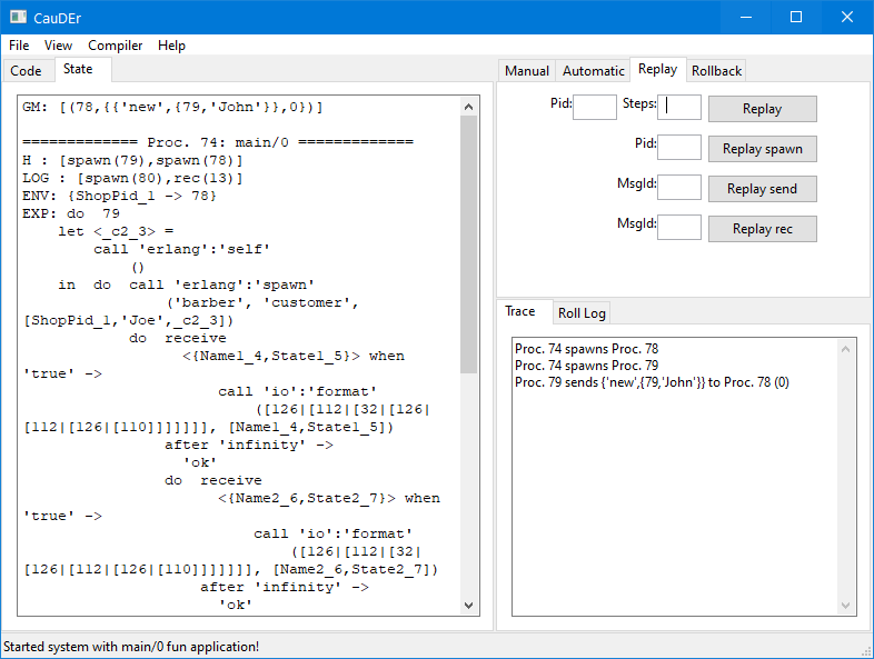
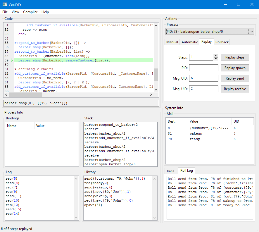
Figure 5: CauDEr Old User Interface vs New Interface

The controlled semantics is the basis of the implemented reversible debugger CauDEr. Figure 5 shows a snapshot of both the old and the new, improved user interface. In contrast to the previous version of the debugger [9], we show the source code of the program and highlight the line that is being evaluated. In contrast, the old version showed the current Core Erlang expression to be reduced, which was far less intuitive. Moreover, all the available information (bindings, stack, log, history, etc) is shown in different boxes, while the previous version showed all information together in a single text box. Furthermore, the user can now decide whether to add a log or not, while the previous version required the use of different implementations of the debugger.

The new version of the reversible debugger is publicly available from https://github.com/mistupv/cauder.

4 Conclusions and Future Work

In this paper, we have adapted and extended the framework for causal-consistent reversible debugging from Core Erlang to Erlang. In doing so, we have extended the standard semantics to also cope with program constructs that were not covered in previous work [8, 7, 10], e.g., if statements, higher-order functions, sequences, etc. Furthermore, we have integrated user-driven debugging and replay debugging into a single, more general framework. Finally, the user interface of CauDEr has been redesigned in order to make it easier to use (and closer to that of the standard debugger of Erlang). We refer the reader to [8, 10] for a detailed comparison between causal-consistent reversible debugging in Erlang and other, related work.

As for future work, we aim at modelling in the semantics different levels of granularity for debugging. For instance, the user may choose to evaluate a function call in one step or to explore the reduction of the function’s body step by step. Moreover, we are also exploring the possibility of allowing the user to speculatively receive a message which is different from the one in the process’ log during replay debugging. Finally, other interesting ideas for future work include the implementation of appropriate extensions to deal with distributed programs and error handling (following, e.g., the approach of [6]).

Acknowledgements.

The authors would like to thank Ivan Lanese for his useful remarks that helped us to improve the new version of the CauDEr debugger.

Appendix 0.A The Language Syntax

In this section, we present the complete syntax of the considered language: a significant subset of the higher-order functional and concurrent programming language Erlang.

$\begin{array}[]{rcl@{~~~}rcl}\mathit{program}&::=&\mathit{mod}_{1}~{}\ldots~{}\mathit{mod}_{n}\hfil~{}~{}~{}\\ \mathit{mod}&::=&\mathit{fun\_def}_{1}~{}\ldots~{}\mathit{fun\_def}_{n}\hfil~{}~{}~{}\\ \mathit{fun\_def}&::=&\mathit{fun\_rule}~{}\{^{\prime};^{\prime}~{}\mathit{fun\_rule}\}~{}^{\prime}.^{\prime}\hfil~{}~{}~{}\\ {\mathit{fun\_rule}}&::=&\mathit{Atom}([\mathit{exprs}])~{}[\mathsf{when}~{}\mathit{guard}]\to\mathit{exprs}\hfil~{}~{}~{}\\ \mathit{fun\_expr}&::=&\mathsf{fun}~{}\mathit{fun}~{}\{^{\prime};^{\prime}~{}\mathit{fun}\}~{}\mathsf{end}\hfil~{}~{}~{}\\ {\mathit{fun}}&::=&([\mathit{exprs}])~{}[\mathsf{when}~{}\mathit{guard}]\to\mathit{exprs}\hfil~{}~{}~{}\\ \mathit{pattern}&::=&\mathit{atomic}\mid\mathit{Var}\mid~{}^{\prime}\{^{\prime}[\mathit{patterns}]^{\prime}\}^{\prime}\mid~{}^{\prime}[^{\prime}~{}[\mathit{patterns}~{}^{\prime}|^{\prime}\mathit{pattern}]~{}^{\prime}]^{\prime}\hfil~{}~{}~{}\\ \mathit{patterns}&::=&\mathit{pattern}~{}\{^{\prime},^{\prime}~{}\mathit{pattern}\}\hfil~{}~{}~{}\\ \mathit{exprs}&::=&\mathit{expr}~{}\{^{\prime},^{\prime}~{}\mathit{expr}\}\hfil~{}~{}~{}\\ \mathit{expr}&::=&\mathit{atomic}\mid\mathit{Var}\mid~{}^{\prime}\{^{\prime}[\mathit{exprs}]^{\prime}\}^{\prime}\mid~{}^{\prime}[^{\prime}~{}[\mathit{exprs}~{}^{\prime}|^{\prime}\mathit{expr}]~{}^{\prime}]^{\prime}\mid\mathsf{if}~{}\mathit{if\_clauses}~{}\mathsf{end}\hfil~{}~{}~{}\\ &\mid&\mathsf{case}~{}expr~{}\mathsf{of}~{}\mathit{cr\_clauses}~{}\mathsf{end}\mid\mathsf{receive}~{}\mathit{cr\_clauses}~{}\mathsf{end}\mid\mathit{expr}~{}!~{}\mathit{expr}\hfil~{}~{}~{}\\ &\mid&\mathit{pattern}=\mathit{expr}\mid[\mathit{Mod}\!:]\mathit{expr}([\mathit{exprs}])\mid\mathit{fun\_expr}\mid Opexprs\hfil~{}~{}~{}\\ \mathit{atomic}&::=&\mathit{Atom}\mid\mathit{Char}\mid\mathit{Float}\mid\mathit{Integer}\mid\mathit{String}\hfil~{}~{}~{}\\ \mathit{if\_clauses}&::=&\mathit{guard}~{}\to~{}\mathit{exprs}~{}\{^{\prime};^{\prime}~{}\mathit{guard}~{}\to~{}\mathit{exprs}\}\hfil~{}~{}~{}\\ \mathit{cr\_clauses}&::=&\mathit{pattern}~{}[\mathsf{when}~{}\mathit{guard}]\to\mathit{exprs}~{}\{^{\prime};^{\prime}~{}\mathit{pattern}~{}[\mathsf{when}~{}\mathit{guard}]\to\mathit{exprs}\}\hfil~{}~{}~{}\\ \end{array}$

Figure 6: Language syntax rules

The syntax of the language is shown in Figure 6. Terminals are denoted with sans serif font or using single quotes. We distinguish expressions, patterns, and values. Patterns are built from variables, literals (atomic values), lists, and tuples; they can only contain fresh variables. In contrast, values are built from literals, lists, and tuples, i.e., they are ground (without variables) patterns. Expressions are ranged over by $e,e^{\prime},e_{1},\ldots$, patterns by $pat$, $pat^{\prime}$, $pat_{1}$, $\ldots$ and values by $v,v^{\prime},v_{1},\ldots$ Atoms (i.e., constants with a name) are written in roman letters, while variables start with an uppercase letter.

A program is a collection of modules, where each module includes a sequence of function definitions, A function is defined by one or more clauses of the form $f(pat_{1},\ldots,pat_{n})\to e_{1},\ldots,e_{m}$, where $f$ is an atom. Note that clauses can have a sequence of expressions in the right-hand side. Clauses are tried from top to bottom using pattern matching. Morever, clauses may have a guard (prefixed by the keyword when) that must be evaluated to $\mathsf{true}$ in order for the rule to be applicable. Guards can only contain calls to predefined functions (typically, relational and arithmetic operators). An expression can include atomic values, variables, tuples of the form $\{e_{1},\ldots,e_{n}\}$, lists (using Prolog-like notation, where $[\>]$ is the empty list and $[e_{1}|e_{2}]$ denotes a list with head $e_{1}$ and tail $e_{2}$), conditionals, case expressions, receive expressions, messsage sending, pattern matching (i.e., expressions of the form $pat=expr$), function applications, anonymous functions, and the usual arithmetic and relational operators. As in Erlang, the only data constructors in the language (besides literals) are the predefined functions for lists and tuples.

Erlang includes a number of built-in functions (BIFs). In this work, we only consider self/0, which returns the process identifier of the current process, and spawn/1 and spawn/3 that creates a new process (see below).

Appendix 0.B The Language Semantics

Now, we present the semantics of the language. As in [8], our operational semantics is defined by means of several layers. The first, lower level layer considers expressions. Here, we distinguish sequential expressions from those related to concurrency. The sequential subset of the language is a typical higher-order eager functional programming language. First, we consider the semantics of sequential expressions.

0.B.1 Sequential Expressions

We need some preliminary notions. A substitution $\theta$ is a mapping from variables to expressions, and ${\mathcal{D}om}(\theta)=\{X\in\mathit{Var}\mid X\neq\theta(X)\}$ is its domain. Substitutions are usually denoted by (finite) sets of bindings like, e.g., $\{X_{1}\mapsto v_{1},\ldots,X_{n}\mapsto v_{n}\}$. Substitutions are extended to morphisms from expressions to expressions in the natural way. The identity substitution is denoted by $id$. Composition of substitutions is denoted by juxtaposition, i.e., $\theta\theta^{\prime}$ denotes a substitution $\theta^{\prime\prime}$ such that $\theta^{\prime\prime}(X)=\theta^{\prime}(\theta(X))$ for all $X\in\mathit{Var}$. We follow a postfix notation for substitution application: given an expression $e$ and a substitution $\sigma$ the application $\sigma(e)$ is denoted by $e\sigma$.

We often denote by $\overline{o_{n}}$ a sequence of syntactic objects $o_{1},\ldots,o_{n}$ for some $n$. We use $\overline{o}$ when the number of objects is not relevant.

In the following, we consider that each expression can be written as $C[e]$ where $e$ is the next redex to be reduced according to the usual eager semantics. E.g., an expression like “$\tt\mathsf{case}~{}f(42)~{}\mathsf{of}~{}\ldots~{}\mathsf{end}$” can be represented as $C[{\tt f(42)}]$ since the call $\tt f(42)$ is needed to evaluate the case expression.

$$\begin{array}[]{c}(\mathit{Var})~{}{\displaystyle\frac{}{\theta,C[X],S\xrightarrow{\tau}\theta,C[\theta(X)],S}\par}\\[17.22217pt] (\mathit{Seq1})~{}{\displaystyle\frac{}{\theta,C[v,e],S\xrightarrow{\tau}\theta,C[e],S}}~{}~{}~{}~{}\par(\mathit{Seq2})~{}{\displaystyle\frac{~{}}{\theta,v,\mathsf{seq}(C[\_])\!:\!S\xrightarrow{\tau}\theta,C[v],S}}\\[17.22217pt] (\mathit{If})~{}{\displaystyle\frac{\mathsf{eval\_guard}(g_{1}\theta,\ldots,g_{n}\theta)=i}{\theta,C[\mathsf{if}~{}g_{1}\to e_{1};\ldots;g_{n}\to e_{n}~{}\mathsf{end}],S\xrightarrow{\tau}\theta,e_{i},\mathsf{seq}(C[\_])\!:\!S}}\\[17.22217pt] (\mathit{Case})~{}{\displaystyle\frac{\mathsf{match\_case}(v,cl_{1}\theta,\ldots,cl_{n}\theta)=\langle\theta_{i},e_{i}\rangle}{\theta,C[\mathsf{case}~{}v~{}\mathsf{of}~{}cl_{1};\ldots;cl_{n}~{}\mathsf{end}],S\xrightarrow{\tau}\theta\theta_{i},e_{i},\mathsf{seq}(C[\_])\!:\!S}}\\[17.22217pt] (\mathit{Match})~{}{\displaystyle\frac{\mathsf{match}(pat\theta,v)=\sigma}{\theta,C[pat=v],S\xrightarrow{\tau}\theta\sigma,C[v],S}}\\[17.22217pt] (\mathit{Op})~{}{\displaystyle\frac{\mathsf{eval}(op,v_{1},\ldots,v_{n})=v}{\theta,C[op(v_{1},\ldots,v_{n})],S\xrightarrow{\tau}\theta,C[v],S}}\\[17.22217pt] (\mathit{Fun})~{}{\displaystyle\frac{}{\theta,C[\mathsf{fun}~{}\mathit{fun_{1}};\ldots;\mathit{fun_{m}}~{}\mathsf{end}],S\xrightarrow{\tau}\theta,C[\langle\theta,\mathsf{fun}~{}\mathit{fun_{1}};\ldots;\mathit{fun_{m}}~{}\mathsf{end}\rangle],S}}\\[17.22217pt] (\mathit{Call1})~{}{\displaystyle\frac{\mathsf{match\_fun}((v_{1},\ldots,v_{n}),\mathsf{def}(f/n,\mathsf{P}))=(\sigma,e)}{\theta,C[f(v_{1},\ldots,v_{n})],S\xrightarrow{\tau}\sigma,e,(\theta,C[\_])\!:\!S}}\\[17.22217pt] (\mathit{Call2})~{}{\displaystyle\frac{\mathsf{match\_fun}((v_{1},\ldots,v_{n}),\langle\theta^{\prime},\mathsf{fun}~{}\mathit{fun_{1}};\ldots;\mathit{fun_{n}}~{}\mathsf{end}\rangle)=(\sigma,e)}{\theta,C[\langle\theta^{\prime},\mathsf{fun}~{}\mathit{fun_{1}};\ldots;\mathit{fun_{m}}~{}\mathsf{end}\rangle\>(v_{1},\ldots,v_{n})],S\xrightarrow{\tau}\sigma,e,(\theta,C[\_])\!:\!S}}\\[17.22217pt] (\mathit{Return})~{}{\displaystyle\frac{}{\sigma,v,(\theta,C[\_])\!:\!S\xrightarrow{\tau}\theta,C[v],S}\par}\end{array}$$

Figure 7: Standard semantics: evaluation of sequential expressions

The rules for sequential expressions are shown in Figure 7. Our (labeled) reduction semantics is defined on triples $\theta,e,S$, where $\theta$ is the current environment that stores the values of the program variables, $e$ is the expression to be evaluated, and $S$ is a stack. Let us briefly explain the rules of our semantics:

• Rule Var evaluates a variable by simply looking up his value in the environment.

• Rule Seq1 removes a value from a sequence, so that the remaining elements can then be reduced. In general, several Erlang expressions can be reduced to a sequence. Unfortunately, this may give rise to an expression which is syntactically ilegal. Consider, e.g., that the evaluation of the above expression $\tt\mathsf{case}~{}f(42)~{}\mathsf{of}~{}\ldots~{}\mathsf{end}$ reduces $\tt f(42)$ to a sequence like $X=42,X$. Then, we would get the expression $\tt\mathsf{case}~{}X=42,X~{}\mathsf{of}~{}\ldots~{}\mathsf{end}$, which is not syntactically correct (the argument of a case expression must be a single expression, sequences are not allowed). To overcome this problem, rules If and Case move the current context to the stack until the reduced expression is eventually reduced to a single expression and the context is recovered by rule Seq2.

• Rule If evaluates the guards using the auxiliary function $\mathsf{eval\_guard}$, which returns the index of the first guard that evaluates to true. As mentioned above, we move the current context to the stack.

• Rule Case matches the case argument, $v$ with the case branches (possibly including guards) using the auxiliary function $\mathsf{match\_case}$ and returns a pair $\langle\theta_{i},e_{i}\rangle$ with the matching substitution and the expression in the selected branch. As before, the context is moved to the stack to avoid giving rise to an illegal expression if $e_{i}$ is a sequence.

• Rule Match evaluates a pattern matching equation using auxiliary function $\mathsf{match}$, which returns the matching substitution.

• Rule Op evaluates arithmetic and relational operations using the auxiliary function $\mathsf{eval}$.

• Rule Fun evaluates an anonymous function by reducing it to a closure.

• Rules Call1 and Call2 evaluate a function application by moving the current context and environment to the stack and then reducing the function’s body using the auxiliary function match_fun that takes the arguments of the function call and either the definition of the given function in the source program or a closure. Function Return recovers the context and environment from the stack once the function’s body is reduced to a value.

0.B.2 Concurrency

In this section, we consider the semantics of concurrent actions. Essentially, a running application consists of a number of processes that interact by sending and receiving messages. Message sending is asynchronous, while receiving messages may block a process if no (matching) message arrived yet. Processes are uniquely identified by their pid (process identifier).

In principle, one can consider that each process has an associated mailbox or queue where incoming messages are stored until they are consumed by a receive expression. When a process sends a message, it is eventually, stored in the mailbox of the target process. Between the sending of a message and storing it in a process’ mailbox, we say that the message is in the network (which is called the ether in [15]).

In this work, similarly to [10], our semantics abstracts away from processes’ queues. Here, we only consider a single data structure, called global mailbox, that represents both the network and the processes’ mailboxes. Furthermore, the semantics represents an overapproximation of the actual semantics of Erlang since we impose no restriction on the order of messages. In Erlang, the messages between two given processes must arrive in the same order they were sent. We skip this restriction for simplicity (but could easily be implemented, see [12]). Nevertheless, removing this restriction is not relevant in replay mode, since the debugger will follow the trace of an actual execution in some Erlang environment and, thus, only executions that respect the above restriction can be considered.

We note that this contrasts with previous semantics, e.g.,[8, 12, 15], where both the network and the processes’ mailboxes were explicitly modeled.

Let us now introduce the notions of process and system, which are essential in our semantics.

Definition 3 (process)

A process is denoted by a configuration of the form $\langle p,\theta,e,S\rangle$, where $p$ is the pid of the process, $\theta$ is an environment (a substitution of values for variables), $e$ is an expression to be evaluated, and $S$ is an stack.

A so called global mailbox is then used to store sent messages until they are delivered (i.e., consumed by a process using a receive expression):

Definition 4 (global mailbox)

We define a global mailbox, $\Gamma$, as a multiset of triples of the form $(sender\_pid,target\_pid,message)$. Given a global mailbox $\Gamma$, we let $\Gamma\cup\{(p,p^{\prime},v)\}$ denote a new mailbox also including the triple $(p,p^{\prime},v)$, where we use “$\>\cup$” as multiset union.

Finally, a system is defined as follows:

Definition 5 (system)

A system is a pair $\Gamma;\Pi$, where $\Gamma$ is a global mailbox and $\Pi$ is a pool of processes, denoted as $\langle p_{1},\theta_{1},e_{1},S_{1}\rangle~{}\>|\>\cdots\>|\>~{}\langle p_{n},\theta_{n},e_{n},S_{n}\rangle$; here “$\>|\>\!$” represents an associative and commutative operator. We often denote a system as $\Gamma;\langle p,\theta,e,S\rangle\>|\>\Pi$ to point out that $\langle p,\theta,e,S\rangle$ is an arbitrary process of the pool (thanks to the fact that “$\>|\>$” is associative and commutative).

A initial system has the form $\{\>\};\langle p,id,e,[\>]\rangle$, where $\{\>\}$ is an empty global mailbox, $p$ is a pid, $id$ is the identity substitution, $e$ is an expression (typically a function application that starts the execution), and $[\>]$ is an empty stack.

$$\begin{array}[]{r@{~}c}(\mathit{SendExp})~{}&{\displaystyle\frac{}{\theta,C[v_{1}\>!\>v_{2}],S\xrightarrow{\mathsf{send}(v_{1},v_{2})}\theta,C[v_{2}],S}}\\[17.22217pt] (\mathit{ReceiveExp})~{}&{\displaystyle\frac{}{\theta,C[\mathsf{receive}~{}cl_{1};\ldots;cl_{n}~{}\mathsf{end}],S\xrightarrow{\mathsf{rec}(\kappa,\overline{cl_{n}})}\theta,\kappa,\mathsf{seq}(C[\_])\!:\!S}}\\[17.22217pt] (\mathit{SpawnExp1})~{}&{\displaystyle\frac{}{\theta,C[\mathsf{spawn}(mod,f,[\overline{v_{n}}])],S\xrightarrow{\mathsf{spawn}(\kappa,mod,f,[\overline{v_{n}}])}\theta,C[\kappa],S}}\\[17.22217pt] (\mathit{SpawnExp2})~{}&{\displaystyle\frac{}{\theta,C[\mathsf{spawn}(\mathsf{fun}()\to\mathit{exprs}~{}\mathsf{end})],S\xrightarrow{\mathsf{spawn}(\kappa,\mathit{exprs})}\theta,C[\kappa],S}}\\[17.22217pt] (\mathit{SelfExp})~{}&{\displaystyle\frac{}{\theta,C[\mathsf{self}()],S\xrightarrow{\mathsf{self}(\kappa)}\theta,C[\kappa],S}}\end{array}$$

Figure 8: Standard semantics: evaluation expressions with side-effects

$\begin{array}[]{r@{~~}c}(\mathit{Seq})~{}~{}&{\displaystyle\frac{\theta,e,S\xrightarrow{\tau}\theta^{\prime},e^{\prime},S^{\prime}}{\Gamma;\langle p,\theta,e,S\rangle\>|\>\Pi\hookrightarrow_{{\color[rgb]{1,0,0}p,\mathsf{seq}}}\Gamma;\langle p,\theta^{\prime},e^{\prime},S^{\prime}\rangle\>|\>\Pi}}\\[12.91663pt] (\mathit{Send})~{}~{}&{\displaystyle\frac{\theta,e,S\xrightarrow{\mathsf{send}(p^{\prime},v)}\theta^{\prime},e^{\prime},S^{\prime}~{}\mbox{and}~{}{\color[rgb]{1,0,0}\ell~{}\mbox{is a fresh symbol}}}{\Gamma;\langle p,\theta,e,S\rangle\>|\>\Pi\hookrightarrow_{{\color[rgb]{1,0,0}p,\mathsf{send}(\ell)}}\Gamma\cup\{(p,p^{\prime},{\color[rgb]{1,0,0}\{v,\ell\}})\};\langle p,\theta^{\prime},e^{\prime},S^{\prime}\rangle\>|\>\Pi}}\\[12.91663pt] (\mathit{Receive})~{}~{}&{\displaystyle\frac{\theta,e,S\xrightarrow{\mathsf{rec}(\kappa,\overline{cl_{n}})}\theta^{\prime},e^{\prime},S^{\prime}~{}~{}\mbox{and}~{}~{}\mathsf{match\_rec}(\overline{cl_{n}}\theta,v)=(\theta_{i},e_{i})}{\Gamma\cup\{(p^{\prime},p,{\color[rgb]{1,0,0}\{v,\ell\}})\};\langle p,\theta,e,S\rangle\>|\>\Pi\hookrightarrow_{{\color[rgb]{1,0,0}p,\mathsf{rec}(\ell)}}\Gamma;\langle p,\theta^{\prime}\theta_{i},e^{\prime}\{\kappa\mapsto e_{i}\},S^{\prime}\rangle\>|\>\Pi}}\\[12.91663pt] (\mathit{Spawn1})~{}~{}&{\displaystyle\frac{\theta,e,S\xrightarrow{\mathsf{spawn}(\kappa,mod,f,[\overline{v_{n}}])}\theta^{\prime},e^{\prime},S^{\prime}~{}~{}\mbox{and}~{}~{}p^{\prime}~{}\mbox{is a fresh pid}}{\Gamma;\langle p,\theta,e,S\rangle\>|\>\Pi\hookrightarrow_{{\color[rgb]{1,0,0}p,\mathsf{spawn}(p^{\prime})}}\Gamma;\langle p,\theta^{\prime},e^{\prime}\{\kappa\mapsto p^{\prime}\},S^{\prime}\rangle\>|\>\langle p^{\prime},id,mod\!:\!f(\overline{v_{n}}),[\>]\rangle\>|\>\Pi}}\\[12.91663pt] (\mathit{Spawn2})~{}~{}&{\displaystyle\frac{\theta,e,S\xrightarrow{\mathsf{spawn}(\kappa,\mathit{exprs}])}\theta^{\prime},e^{\prime},S^{\prime}~{}~{}\mbox{and}~{}~{}p^{\prime}~{}\mbox{is a fresh pid}}{\Gamma;\langle p,\theta,e,S\rangle\>|\>\Pi\hookrightarrow_{{\color[rgb]{1,0,0}p,\mathsf{spawn}(p^{\prime})}}\Gamma;\langle p,\theta^{\prime},e^{\prime}\{\kappa\mapsto p^{\prime}\},S^{\prime}\rangle\>|\>\langle p^{\prime},id,\mathit{exprs},[\>]\rangle\>|\>\Pi}}\\[12.91663pt] (\mathit{Self})~{}~{}&{\displaystyle\frac{\theta,e,S\xrightarrow{\mathsf{self}(\kappa)}\theta^{\prime},e^{\prime},S^{\prime}}{\Gamma;\langle p,\theta,e,S\rangle\>|\>\Pi\hookrightarrow_{{\color[rgb]{1,0,0}p,\mathsf{self}}}\Gamma;\langle p,\theta^{\prime},e^{\prime}\{\kappa\mapsto p\},S^{\prime}\rangle\>|\>\Pi}}\end{array}$

Figure 9: Tracing semantics

The transition rules for concurrent expressions is shown in Figure 8, while the (labeled) transition rules for systems is shown in Figure 9. For the moment, the reader can safely ignore the labels of the arrows. Let us briefly explain how concurrent expressions and systems are evaluated:

• First, a system in which the selected process has a sequential expression (i.e., an expression that can be reduced using the rules of Figure 7) is evaluated using rule Seq in Figure 9 in the obvious way.

• Sending a message. On the one hand, rule SendExp reduces an expression $v_{1}\>!\>v_{2}$ (i.e., sending message $v_{2}$ to process with pid $v_{1}$) to $v_{2}$. However, we also need some side-effect: message $v_{2}$ must be eventually received by process $v_{1}$. Since this is not observable locally, we label the step with $\mathsf{send}(v_{1},v_{2})$ so that rule Send can take care of this by adding the triple $(p,p^{\prime},\{v,l\})$ to the global mailbox $\Gamma$, where $p$ is the pid of the sender, $p^{\prime}$ is the pid of the target, and $\{v,\ell\}$ is a tagged message. Here, messages are tagged with unique labels so that we can connect messages sent and received without ambiguity. Note that without unique labels, messages with the same value would be indistinguishable.

• Receiving a message. At the level of expressions, rule ReceiveExp returns a fresh variable, $\kappa$, since the receive expression cannot be reduced at this level without accessing to the global mailbox. Here, $\kappa$ can be seen as a future that will be bound in the next layer of the semantics. As before, we label the step with enough information for rule Receive to complete the reduction. This rule looks for some (in principle, arbitrary) message addressed to the considered process in the global mailbox, checks that it matches some branch of the receive expression using the auxiliary function $\sf match\_rec$, and then proceeds as in the evaluation of a case expression. The main difference is that, now, $\kappa$ is bound to the selected branch and the message is removed from the global mailbox.

• Spawning a process. For spawning a process, we proceed analogously to the previous case. Rules SpawnExp1 and SpawnExp2 labels the step with the appropriate information and the calls are reduced to a fresh variables $\kappa$. Then, rules Spawn1 and Spawn2 perform the corresponding side effect (creating a new process) and bind $\kappa$ to the pid of the new process.

• Finally, $\mathsf{self}()$ returns the pid of the current process using rule SelfExp and Self, analogously to the previous cases.

We refer to reduction steps derived by the system rules as actions taken by the chosen process.

Finally, by considering the labels in the transition steps of the semantics shown in Figure 9, we get a tracing semantics that produces the log of a computation. This log can then be used in the debugger to replay a (typically faulty) computation. Let us note that, in practice, we use a program instrumentation rather than an instrumented semantics, so that the instrumented program can be executed in the standard Erlang/OTP environment. The equivalence between the two alternatives is rather straightforward though.

In the following, (ordered) sequences are denoted by $w=(r_{1},r_{2},\ldots,r_{n})$, $n\geq 1$, where $[\>]$ denotes the empty sequence. Given sequences $w_{1}$ and $w_{2}$, we denote their concatenation by $w_{1}\mbox{$+$}w_{2}$; when $w_{1}$ just contains one element, i.e., $w_{1}=(r)$, we write $r\mbox{$+$}w_{2}$ instead of $(r)\mbox{$+$}w_{2}$ for simplicity.

Definition 6 (log)

A log is a (finite) sequence of events $(r_{1},r_{2},\ldots)$ where each $r_{i}$ is either $\mathsf{spawn}(p)$, $\mathsf{send}(\ell)$ or $\mathsf{rec}(\ell)$, with $p$ a pid and $\ell$ a message identifier. Logs are ranged over by $\omega$. Given a derivation $d=(s_{0}\hookrightarrow_{p_{1},r_{1}}s_{1}\hookrightarrow_{p_{2},r_{2}}\ldots\hookrightarrow_{p_{n},r_{n}}s_{n})$, $n\geq 0$, under the logging semantics, the log of a process $p$ in $d$, in symbols $\mathcal{L}(d,p)$, is inductively defined as follows:

$$\mathcal{L}(d,p)=\left\{\begin{array}[]{l@{~~~}l}[\>]\hfil~{}~{}~{}&\mbox{if}~{}n=0~{}\mbox{or}~{}p~{}\mbox{does not occur in}~{}d\\ r_{1}\mbox{$+$}\mathcal{L}(s_{1}\hookrightarrow^{\ast}s_{n},p)\hfil~{}~{}~{}&\mbox{if}~{}n>0,~{}p_{1}=p,~{}\mbox{and}~{}r_{1}\not\in\{\mathsf{seq},\mathsf{self}\}\\ \mathcal{L}(s_{1}\hookrightarrow^{\ast}s_{n},p)\hfil~{}~{}~{}&\mbox{otherwise}\\ \end{array}\right.$$

The log of $d$, written $\mathcal{L}(d)$, is defined as: $\mathcal{L}(d)=\{(p,\mathcal{L}(d,p))\mid\mbox{$p$ occurs in $d$}\}$. We sometimes call $\mathcal{L}(d)$ the system log of $d$ to avoid confusion with $\mathcal{L}(d,p)$ (the process’ log). Trivially, $\mathcal{L}(d,p)$ can be obtained from $\mathcal{L}(d)$, i.e., $\mathcal{L}(d,p)=\omega$ if $(p,\omega)\in\mathcal{L}(d)$ and $\mathcal{L}(d,p)=[\>]$ otherwise.

Clearly, given a finite derivation $d$, the associated log $\mathcal{L}(d)$ is finite too. However, the opposite is not true: we might have a finite log associated to an infinite derivation (e.g., by applying infinitely many times rule $\mathit{Seq}$).

References

-
[1]
Carlsson, R.: An Introduction to Core Erlang. In: Proceedings of the PLI’01
Erlang Workshop (2001), available from
http://www.erlang.se/workshop/carlsson.ps - [2] Giachino, E., Lanese, I., Mezzina, C.A.: Causal-consistent reversible debugging. In: Gnesi, S., Rensink, A. (eds.) Proceedings of the 17th International Conference on Fundamental Approaches to Software Engineering (FASE 2014). Lecture Notes in Computer Science, vol. 8411, pp. 370–384. Springer (2014)
- [3] Grishman, R.: The debugging system AIDS. In: American Federation of Information Processing Societies: AFIPS Conference Proceedings: 1970 Spring Joint Computer Conference. AFIPS Conference Proceedings, vol. 36, pp. 59–64. AFIPS Press (1970), https://doi.org/10.1145/1476936.1476952
- [4] Lamport, L.: Time, clocks, and the ordering of events in a distributed system. Commun. ACM 21(7), 558–565 (1978)
- [5] Landauer, R.: Irreversibility and heat generation in the computing process. IBM Journal of Research and Development 5, 183–191 (1961)
- [6] Lanese, I., Medic, D.: A general approach to derive uncontrolled reversible semantics. In: Konnov, I., Kovács, L. (eds.) 31st International Conference on Concurrency Theory, CONCUR 2020, September 1-4, 2020, Vienna, Austria (Virtual Conference). LIPIcs, vol. 171, pp. 33:1–33:24. Schloss Dagstuhl - Leibniz-Zentrum für Informatik (2020), https://doi.org/10.4230/LIPIcs.CONCUR.2020.33
- [7] Lanese, I., Nishida, N., Palacios, A., Vidal, G.: CauDEr: A Causal-Consistent Reversible Debugger for Erlang (system description). In: Gallagher, J.P., Sulzmann, M. (eds.) Proceedings of the 14th International Symposium on Functional and Logic Programming (FLOPS’18). Lecture Notes in Computer Science, vol. 10818, pp. 247–263. Springer (2018)
- [8] Lanese, I., Nishida, N., Palacios, A., Vidal, G.: A theory of reversibility for Erlang. Journal of Logical and Algebraic Methods in Programming 100, 71–97 (2018)
- [9] Lanese, I., Nishida, N., Palacios, A., Vidal, G.: CauDEr website. URL: https://github.com/mistupv/cauder (2019)
- [10] Lanese, I., Palacios, A., Vidal, G.: Causal-consistent replay debugging for message passing programs. In: Pérez, J.A., Yoshida, N. (eds.) Proceedings of the 39th IFIP WG 6.1 International Conference on Formal Techniques for Distributed Objects, Components, and Systems (FORTE 2019). Lecture Notes in Computer Science, vol. 11535, pp. 167–184. Springer (2019)
- [11] Leroy, X., Doligez, D., Frisch, A., Garrigue, J., Rémy, D., Vouillon, J.: The OCaml system release 4.11. Documentation and user’s manual. Tech. rep., INRIA (2020)
- [12] Nishida, N., Palacios, A., Vidal, G.: A reversible semantics for Erlang. In: Hermenegildo, M., López-García, P. (eds.) Proceedings of the 26th International Symposium on Logic-Based Program Synthesis and Transformation (LOPSTR 2016). Lecture Notes in Computer Science, vol. 10184, pp. 259–274. Springer (2017)
- [13] Nishida, N., Palacios, A., Vidal, G.: Reversible computation in term rewriting. J. Log. Algebraic Methods Program. 94, 128–149 (2018), https://doi.org/10.1016/j.jlamp.2017.10.003
- [14] O’Callahan, R., Jones, C., Froyd, N., Huey, K., Noll, A., Partush, N.: Engineering record and replay for deployability: Extended technical report. CoRR abs/1705.05937 (2017), http://arxiv.org/abs/1705.05937
- [15] Svensson, H., Fredlund, L.A., Earle, C.B.: A unified semantics for future Erlang. In: 9th ACM SIGPLAN workshop on Erlang. pp. 23–32. ACM (2010)
- [16] Undo Software: Increasing software development productivity with reversible debugging (2014), https://undo.io/media/uploads/files/Undo_ReversibleDebugging_Whitepaper.pdf
- [17] Zelkowitz, M.V.: Reversible execution. Commun. ACM 16(9), 566 (1973), https://doi.org/10.1145/362342.362360