Hierarchical Features Matter: A Deep Exploration of GAN Priors for Improved Dataset Distillation

Abstract

Dataset distillation is an emerging dataset reduction method, which condenses large-scale datasets while maintaining task accuracy. Current methods have integrated parameterization techniques to boost synthetic dataset performance by shifting the optimization space from pixel to another informative feature domain. However, they limit themselves to a fixed optimization space for distillation, neglecting the diverse guidance across different informative latent spaces. To overcome this limitation, we propose a novel parameterization method dubbed Hierarchical Generative Latent Distillation (H-GLaD), to systematically explore hierarchical layers within the generative adversarial networks (GANs). This allows us to progressively span from the initial latent space to the final pixel space. In addition, we introduce a novel class-relevant feature distance metric to alleviate the computational burden associated with synthetic dataset evaluation, bridging the gap between synthetic and original datasets. Experimental results demonstrate that the proposed H-GLaD achieves a significant improvement in both same-architecture and cross-architecture performance with equivalent time consumption.

1 Introduction

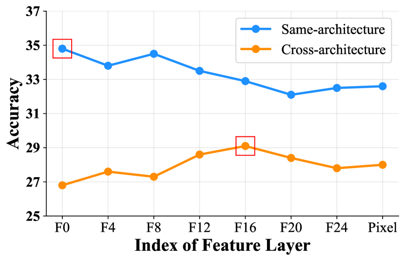
Figure 1: Performance of synthetic datasets condensed from various feature domains provided by GAN under the same settings (DC on ImageNet-Birds).

In recent years, deep learning has made significant strides in various research fields, encompassing computer vision [1, 2] and natural language processing [3, 4]. These advancements have been facilitated by utilizing larger and more intricate deep neural networks (DNNs) in conjunction with numerous datasets tailored for diverse application fields. However, as the complexity of various learning tasks increases, neural networks have grown both deeper and wider, resulting in an exponential surge in the size of datasets required for training these models. This has presented a substantial challenge to data storage and processing efficiency [5], further exacerbating the bottleneck in deep learning due to the mismatch between the enormous data volume and limited computing resources.

Dataset distillation (DD) [6] has emerged as a promising solution to the aforementioned issues. It allows for the generation of a more compact synthetic dataset, where each data point encapsulates a higher concentration of task-specific information than its real counterparts. When trained on the synthetic dataset, the network can achieve performance comparable to its counterpart using the original dataset. By significantly reducing the size of the training data, dataset distillation offers a substantial reduction in training costs and memory consumption. Various methods have been proposed to enhance the performance of the condensed dataset. Early studies minimized the distance metric between synthetic and real datasets by directly optimizing the image pixels [7, 8, 9]. Subsequently, synthetic dataset parameterization methods [10, 11, 12, 13] employ differentiable operations to process synthetic images, shifting the optimization space from pixels to feature domains. These methods benefit from the efficient guidance of hidden features, thus achieving better performance. However, existing parameterization methods focus on one fixed optimization space, overlooking the informative guidance across multiple corresponding feature domains.

FreD [13] optimizes the synthetic dataset in the low-frequency space using discrete cosine transform (DCT), while HaBa [11] optimizes the synthetic dataset in the feature space of a small neural network called allucinator network. However, FreD ignores informative guidance in the high-frequency domain provided by DCT and HaBa only regards the allucinator network as a holistic counterpart. On the other hand, several recent studies have exploited the rich semantic information encoded in different spaces within the generators [10, 12] for enhanced parameterization distillation results. ITGAN[10] directly optimizes the initial latent space of GAN and achieves significant performance improvements on low-resolution datasets. To fully utilize the GAN prior, GLaD [12] decomposes the GAN structure and manually select the intermediate layer, greatly enhancing the cross-architecture performance of the synthetic dataset. However, this strategy exhibits a performance decrease in the same-architecture settings when coupled with certain dataset distillation methods as suggested in Figure 1. In this manner, even though synthetic datasets are condensed from the optimally selected intermediate layer through preliminary experiments by manual picking, the diverse model architectures still lead to changes in the optimal performance. As aforementioned parameterization methods, current GAN-based approaches limit the optimization space to a specific feature domain and necessitate extensive computing time and resources to manually select the optimal feature domain for different settings. This naturally raises a question: Does a fixed optimization space meet the demands of dynamic data distribution and model architectures during parameterization dataset distillation?

To address this question, we propose a straightforward and efficient approach based on parameterization method using GANs as prior, Hierarchical Generative Latent Distillation (H-GLaD), which explores the significance of hierarchical features and offers a more profound exploration of GAN priors to enhance dataset distillation. The proposed H-GLaD embraces adaptive exploration across all hierarchical feature domains within GAN models. Specifically, we decompose the GAN structure, undertaking a greedy search that spans different hierarchical feature domains. During the distillation process, we optimize these hierarchical latents within the GAN model, guided by the loss from the dataset distillation task. Throughout this optimization, we track the best hierarchical latents at the current layer, feeding them into the next layer. This iterative process continues until the optimizer traverses the hierarchical layers and reaches the pixel domain. To mitigate the time-consuming nature of performance evaluation, we introduce a class-relevant feature distance metric between the synthetic dataset and the real dataset to search the optimal latent feature. This metric serves as a performance estimation for the synthetic datasets, encapsulating the significance of hierarchical features. Crucially, our method explores hierarchical features more comprehensively than previous approaches, which only relied on a single fixed feature domain as image priors.

The main contributions can be summarized as follows:

• Our method effectively harnesses informative guidance from the hierarchical feature domains of pre-trained GAN models, providing a novel parametrization framework to enhance their efficiency by leveraging information across various feature domains.

• By systematically exploring GAN’s feature space at each layer, we improve both the cross-architecture and same-architecture performance of the synthetic dataset.

• To mitigate the computational demands associated with searching feature domains, we introduce a novel class-relevant feature distance metric, saving valuable computational time by approximating the real performance of the synthetic dataset.

2 Related Works

2.1 Dataset Distillation

Dataset distillation was initially regarded as a meta-learning problem [6]. It involves minimizing the loss function of the synthetic dataset using a model trained on the synthetic dataset. Since then, several approaches have been proposed to enhance the performance of dataset distillation. One category of methods utilizes ridge regression models to approximate the inner loop optimization [16, 17, 18, 19]. Another category of methods selects an informative space as a proxy target to address the unrolled optimization problem. DC [7], DSA [20] and DCC [21] match the weight gradients of models trained on the real and synthetic dataset, while DM [9] and CAFE [22] use feature distance between the real and synthetic dataset as matching targets. MTT [8] and TESLA [23] match the model parameter trajectories obtained from training on the real dataset and the synthetic dataset. In recent years, some studies have argued that the bi-level optimization structure required by traditional dataset distillation is redundant and computationally expensive.Following DM, DataDAM [24] and IDM[25] solely relies on the proxy information of the synthetic and real datasets extracted by multiple untrained models, thereby eliminating the need for the bi-level optimization structure. Other studies suggest that the pixel domain, where images reside, is considered a high-dimensional space. Therefore, performance improvement can be achieved by parameterizing the synthetic dataset and transferring the optimization space. IDC [26] and HaBa [11] perform optimization in a low-dimensional space using differentiable operations, while GLaD [12] and ITGAN [10] utilize the feature domain provided by GANs as the optimization space, both of them employ pre-trained GANs as priors. FreD [13] employs traditional compression methods (e.g., DCT) to provide a low-frequency space as the optimization space.

The proposed H-GLaD introduces an innovative approach to parameterizing synthetic datasets through GANs. This method represents a broader and more encompassing enhancement compared to previous approaches utilizing generative models as priors.

2.2 GAN as prior

GAN [27] is a deep generative model trained adversarially to learn the distribution of real images. Recent studies have shown that GANs can tackle inverse problems by mapping images into their latent space [15, 28, 29, 30, 37], enabling tasks like image editing [31, 32]. Incorporating image distribution information into GAN enhances the performance of dataset distillation by utilizing GAN to parameterize the synthetic dataset. ITGAN proposes using GAN (e.g., BigGAN [33]) as image priors for the image dataset, using the initial feature domain of GANs as the optimization space to boost performance. However, this approach requires converting the entire real dataset into latent using GANs’ inverse method, incurring unacceptable time costs for high-resolution and large-scale datasets. GLaD also employs GAN (e.g., StyleGAN-XL [34]) as a prior and significantly improves the cross-architecture performance of the synthetic dataset by selecting the feature domain of GAN’s intermediate layers as the optimization space. However, it overlooks the fact that the optimal optimization space may vary when dealing with different datasets, even with the same dataset distillation method. Additionally, it ignores the guidance offered by GAN’s earlier layers.

Similar to the successful application of intermediate layer optimization in various fields [35, 36], our method addresses these limitations by not restricting the optimization space to a specific feature domain provided by GANs. Instead, we explore hierarchical feature domains of GANs, resulting in an optimization method that does not require pre-determining the optimization space and incorporates all guidance information from the GAN priors.

3 Method

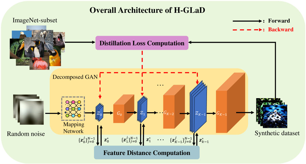
Figure 2: Framework of the proposed H-GLaD, which outlines the synthesis of a hierarchical synthetic dataset using decomposed GAN layers. The lower part details the search for hierarchical layers, utilizing a layer-wise feature distance to find optimal latent features and generate the synthetic dataset.

In this section, we first present the problem definition of dataset distillation and discuss existing methods that parameterize synthetic datasets using GANs. Subsequently, we delve into the specifics of our method, aiming to improve upon previous works by exploring the feature domains provided by GANs. Finally, we propose an alternative evaluation scheme that assesses the synthetic dataset’s performance by measuring the layer-wise feature distance between it and the real one. The overview of our approach is depicted in Figure 2.

3.1 Preliminaries

Dataset distillation necessitates a real large-scale dataset $\mathcal{T}=\{(\mathbf{x}_{t}^{i},y_{t}^{i})\}_{i=1}^{\mathcal{T}}$ and aims to create a smaller synthetic dataset $\mathcal{S}=\{(\mathbf{x}_{s}^{i},y_{s}^{i})\}_{i=1}^{\mathcal{S}}$ ($\left|\mathcal{S}\right|\ll\left|\mathcal{T}\right|$), minimizing the performance gap between models trained on the two datasets. To achieve this, a well-designed matching objective $\phi(\cdot)$ is employed to extract feature distances in a specific informative space, representing the performance gap between the real and synthetic datasets. The optimization process involves initializing the synthetic dataset from the real dataset and iteratively updating it by minimizing the feature distance, which can be formulated below:

$$\mathcal{S}^{*}=\mathop{\arg\min}\limits_{\mathcal{S}}\mathcal{M}(\phi(\mathcal{S}),\phi(\mathcal{T})),$$ (1)

where $\mathcal{M}(\,\cdot,\cdot\,)$ denotes some matching metric, e.g., neural network gradients [7], exacted features[9], and training trajectories[8].

Building upon these findings, methods that parameterize synthetic datasets shift the optimization space from the pixel domain to the feature domain by employing differentiable operations. For instance, GAN priors-based methods [10, 12] can be formulated uniformly below:

$$\mathbf{z}^{*}=\mathop{\arg\min}\limits_{\mathbf{z}\in\mathcal{Z}}\mathcal{M}(\phi(G_{w}(\mathbf{z})),\phi(\mathcal{T})),$$ (2)

where $\mathbf{z}\in\mathcal{Z}$ represents the latent in a specific feature domain of a pre-trained generative model $G_{w}(\,\cdot\,)$. Guided by GAN priors, these methods demonstrate substantial performance improvements.

3.2 Progressive Optimization with Hierarchical Feature Domains

As depicted in Algorithm 1, our approach diverges from restricting the optimization space to a specific feature domain of the GANs. Instead, we aim to explore the hierarchical layers of the GAN, striving to enhance the effective utilization of the prior information.

Algorithm 1 Pseudocode of the proposed H-GLaD

Input: $G_{w}(\,\cdot\,)$: a pre-trained generative model; $K$: the number of hierarchical layers; $N$: distillation steps; $\mathcal{T}$: real training dataset; $P_{z}$: distribution of latent initializations; $\mathcal{L}$: distillation loss; $Acc(\,\cdot\,)$: evaluate real performance of synthetic dataset;

1:  Initial average latent $\mathbf{z}\sim P_{\mathcal{Z}}$

2:  Dissemble $G_{w}(\,\cdot\,)$ into $G_{k-1}\circ G_{k-2}\circ\cdots\circ G_{0}(\,\cdot\,)$

3:  $acc_{max}=0$

4:  for i ${\leftarrow}$ 0 to $K-1$ do

5:     $d_{min}=\mathcal{D}(G_{k-1}\circ\cdots\circ G_{i}(\mathbf{z}_{i}^{0}),\mathcal{T})$

6:     for j ${\leftarrow}$ 0 to $N-1$ do

7:        $\mathcal{S}_{i}^{j}=G_{k-1}\circ\cdots\circ G_{i}(\mathbf{z}_{i}^{j})$.

8:        $\mathcal{L}=\mathcal{M}(\phi(\mathcal{S}_{i}^{j}),\phi(\mathcal{T}))$

9:        $\mathbf{z}_{i}^{j+1}\leftarrow SGD(\mathbf{z}_{i}^{j};\mathcal{L})$

10:        if $\mathcal{D}(\mathcal{S}_{i}^{j},\mathcal{T})\leq d_{min}$ then

11:           $\mathbf{z}_{i}^{*}=\mathbf{z}_{i}^{j},\mathcal{S}_{i}^{*}=\mathcal{S}_{i}^{j}$

12:        end if

13:     end for

14:     if $Acc(\mathcal{S}_{i}^{*})>acc_{max}$ then

15:        $acc_{max}=Acc(\mathcal{S}_{i}^{*})$

16:        $\mathcal{S}=\mathcal{S}_{i}^{*}$

17:     end if

18:     $\mathbf{z}_{i+1}^{0}=G_{i}(\mathbf{z}_{i}^{*})$

19:  end for

Output: Synthetic dataset $\mathcal{S}$

To sufficiently utilize the informative guidance from the hierarchical feature domains, we decompose a pre-trained GAN $G_{w}(\cdot)$ for hierarchical layer searching, i.e.,

$$G_{w}(\,\cdot\,)=G_{K-1}\circ G_{K-2}\circ\cdots\circ G_{1}\circ G_{0}(\,\cdot\,).$$ (3)

For each hierarchical layer $G_{i}$ provided by GAN, we repeat the following steps. Firstly, we generate images from $\mathbf{z}_{i}$ only using the remaining synthesizing network $G_{k-1}(\,\cdot\,)\circ G_{k-2}(\,\cdot\,)\circ\cdots\circ G_{i}(\,\cdot\,)$. Then, we employ the distillation method (e.g., MTT [8]) to calculate $\mathcal{L}$ based on the synthetic dataset composed of generated images and the real dataset to optimize $\mathbf{z}_{i}$ with an SGD optimizer, the optimization process lasts for a pre-determined and fixed $N$ steps. After completing the optimization process for a specific layer, we implicitly evaluate the latents synthesized during the SGD optimization process and record $\mathbf{z}_{i}^{*}$ as the optimal latents for the current layer. Finally, we pass $\mathbf{z}_{i}^{*}$ into the next layer to obtain $\mathbf{z}_{i+1}^{0}$ as the initial latent for the next layer.

When the optimization space reaches the ultimate pixel domain, we choose the optimal latent $\mathbf{z}^{*}$ from the recorded latents $\mathbf{z}_{i}^{*}$ based on the real performance of the synthetic dataset $\mathcal{S}$ generated by the corresponding remaining synthesizing network $G_{k-1}(\,\cdot\,)\circ G_{k-2}(\,\cdot\,)\circ\cdots\circ G_{i}(\,\cdot\,)$. In this way, we fully explore the feature domain of the GAN, leveraging its rich information.

3.3 Enhancing Performance with Efficient Searching Strategy

Ensemble-Averaging Latent Initialization

To mitigate the undesirable time overhead brought by existing methods [38] using clustering or GAN inversion [15], we propose an inactive searching initialization by calculating the average value of multiple noises, and passing it through the GAN’s mapping network to obtain the initial latent $\mathbf{z}_{0}$ with reduced bias. our method showcases simplicity without compromising effectiveness, as confirmed by experimental results as shown in Section 4.4.

Class-relevant Feature Distance

To search for optimal latent as the optimization starting point of the subsequent feature domain, an efficient implicit evaluation metric is needed to replace the time-consuming evaluation of the synthetic dataset’s real performance. We first attempt to use the loss value as a substitute evaluation metric. However, it fails to yield desired results and, in some cases, performs even worse than not searching at all.

To utilize gradient information while maintaining diversity, we adopt the class activation map (CAM)[39] by utilizing the gradients of the corresponding class with respect to the feature maps to localize the class-specific features. With the output logits $q={f}^{d}({w}^{d};\mathbf{z})$ from the classifier ${w}^{d}$, the CAM is defined as the gradients of output logits ${q}^{y}$ of class $y$ with respect to features $\mathbf{z}$ at as follows:

$${g}_{\mathbf{z}}=\frac{\partial{q}^{y}}{\partial\mathbf{z}}.$$ (4)

To focus attention on the class-relevant region, we propose a novel class-relevant feature distance $\mathcal{D}(\mathcal{S},\mathcal{T})$ between the real dataset $\mathcal{S}$ and the synthetic dataset $\mathcal{T}$. i.e.,

$$\mathcal{D}(\mathcal{S},\mathcal{T})=\left\|\frac{1}{|\mathcal{T}|}\sum_{i=1}^{|\mathcal{T}|}{w}^{e}\left(\mathbf{x}_{t}^{i}\right)\cdot\operatorname{ReLU}({g}_{\mathbf{z}}^{t})-\frac{1}{|\mathcal{S}|}\sum_{j=1}^{|\mathcal{S}|}{w}^{e}\left(\mathbf{x}_{s}^{j}\right)\cdot\operatorname{ReLU}({g}_{\mathbf{z}}^{s})\right\|^{2},$$ (5)

where ${w}^{e}$ represents the feature extractor of a pre-trained neural network, and $\operatorname{ReLU}(\cdot)$ is the rectified linear unit function.

4 Experiments

To verify the efficiency of our proposed method, we conduct experiments using code derived from the open-source GLaD. We utilize ImageNet-1K [40] subsets and CIFAR-10 [14] to generate high-resolution and low-resolution distilled datasets respectively, with StyleGAN-XL as the deep generative network. To ensure a fair comparison, we maintain consistency by adopting the same network architecture and employing identical hyperparameters.

4.1 Settings and Implementation Details

Datasets and Network Architectures

In this study, we build upon previous research by utilizing CIFAR10 as low-resolution dataset and ten subsets from ImageNet-1K as high-resolution dataset. These subsets, each consisting of ten categories, are divided into the training and validation sets. They encompass a range of subsets, including traditional subsets like ImageNette and ImageWoof [41], as well as category-specific subsets such as ImageNet-Fruits, ImageNet-Birds, and ImageNet-Cats. Additionally, we introduce subsets named ImageNet-A, ImageNet-B, and so on, each composed of ten categories. These categories are selected based on the descending order of the accuracy achieved by the ResNet-50 [1] model in classification performance on ImageNet-1K. Please refer to Appendix C.1 for the detailed categories included in each dataset.

For the surrogate model for dataset distillation, we choose ConvNet-5 [42] as the backbone network. This network is specifically designed for high-resolution images and consists of five basic blocks and one fully connected layer. Each block includes a $3\times 3$ convolutional layer, instance normalization [43], ReLU non-linear activation, and a $2\times 2$ average pooling layer with a stride of 2. To evaluate the performance of the synthetic dataset, we employ various models, including ConveNet, AlexNet [44], VGG-11 [45], ResNet-18 [1], and a Vision Transformer model [2] from the DC-BENCH [46] resource. It is important to note that all of these evaluation models are versions specifically tailored for corresponding resolution datasets.

4.2 Evaluation Protocol

The approach to assessing the performance of a synthetic dataset is as follows: firstly, a set of models is trained using the synthetic dataset. The training process includes a SGD optimizer with momentum, an approximate and fixed learning rate, and 500 warm-up epochs followed by 500 epochs of cosine decay. Once the training is complete, the trained models are validated using the corresponding validation set from the real dataset. For a specific model architecture, this process is repeated five times, and the average performance is calculated based on these repetitions.

Table 1: Time complexity (min) and performance (%) averaged on ImageNet-[A, B, C, D, E].

Metric	Method	MTT	DC	DM
Time	GLaD	75	69	64
	H-GLaD	70	73	15
perfomance	GLaD	45.0$\pm 0.9$	41.3$\pm 1.2$	37.4$\pm 1.6$
	H-GlaD	50.3$\pm 0.6$	43.2$\pm 0.6$	39.1$\pm 1.2$

In previous studies, the evaluation method involved continuously optimizing the entire distillation process for 1000 epochs, with sampling the synthetic dataset every 100 epochs. The best performance among all sampled examples would then be selected. To ensure a fair performance comparison, we decompose StylGAN-XL into $G_{11}\circ\cdots\circ G_{1}\circ G_{0}(\,\cdot\,)$ and apply the same optimizer and learning rate for each layer, optimizing for 100 steps. This ensures that the total number of optimization epochs remains consistent, thereby preventing performance improvements solely due to a higher number of optimization epochs. The comparison of time complexities and corresponding performance is shown in Table 1.

Simultaneously, the evaluation method used in previous work can be considered a form of uniform sampling. However, our method necessitates an implicit search for the best-performing dataset. Therefore, we adopt the same setup in our evaluation and sample the synthetic dataset after optimizing for 100 epochs in all of these different feature domains (i.e., $\mathbf{z}_{i}^{K-1}$). This approach prevents performance improvements resulting from implicitly selecting a dataset with better performance.

Table 2: Synthetic dataset same-architecture performance (%) on ImageNet-Subset ($128\times 128$) under IPC=1. "Pixel"refers to not deploying GAN.

Alg.	Method	ImNet-A	ImNet-B	ImNet-C	ImNet-D	ImNet-E	ImNette	ImWoof	ImNet-Birds	ImNet-Fruits	ImNet-Cats
	Pixel	51.7$\pm 0.2$	53.3$\pm 1.0$	48.0$\pm 0.7$	43.0$\pm 0.6$	39.5$\pm 0.9$	41.8$\pm 0.6$	22.6$\pm 0.6$	37.3$\pm 0.8$	22.4$\pm 1.1$	22.6$\pm 0.4$
MTT	GLaD	50.7$\pm 0.4$	51.9$\pm 1.3$	44.9$\pm 0.4$	39.9$\pm 1.7$	37.6$\pm 0.7$	38.7$\pm 1.6$	23.4$\pm 1.1$	35.8$\pm 1.4$	23.1$\pm 0.4$	26.0$\pm 1.1$
	H-GLaD	55.1$\pm 0.6$	57.4$\pm 0.3$	49.5$\pm 0.6$	46.3$\pm 0.9$	43.0$\pm 0.6$	45.4$\pm 1.1$	28.3$\pm 0.2$	39.7$\pm 0.8$	25.6$\pm 0.7$	29.6$\pm 1.0$
	Pixel	43.2$\pm 0.6$	47.2$\pm 0.7$	41.3$\pm 0.7$	34.3$\pm 1.5$	34.9$\pm 1.5$	34.2$\pm 1.7$	22.5$\pm 1.0$	32.0$\pm 1.5$	21.0$\pm 0.9$	22.0$\pm 0.6$
DC	GLaD	44.1$\pm 2.4$	49.2$\pm 1.1$	42.0$\pm 0.6$	35.6$\pm 0.9$	35.8$\pm 0.9$	35.4$\pm 1.2$	22.3$\pm 1.1$	33.8$\pm 0.9$	20.7$\pm 1.1$	22.6$\pm 0.8$
	H-GLaD	46.9$\pm 0.8$	50.7$\pm 0.9$	43.9$\pm 0.7$	37.4$\pm 0.4$	37.2$\pm 0.3$	36.9$\pm 0.8$	24.0$\pm 0.8$	35.3$\pm 1.0$	22.4$\pm 1.1$	24.1$\pm 0.9$
	Pixel	39.4$\pm 1.8$	40.9$\pm 1.7$	39.0$\pm 1.3$	30.8$\pm 0.9$	27.0$\pm 0.8$	30.4$\pm 2.7$	20.7$\pm 1.0$	26.6$\pm 2.6$	20.4$\pm 1.9$	20.1$\pm 1.2$
DM	GLaD	41.0$\pm 1.5$	42.9$\pm 1.9$	39.4$\pm 1.7$	33.2$\pm 1.4$	30.3$\pm 1.3$	32.2$\pm 1.7$	21.2$\pm 1.5$	27.6$\pm 1.9$	21.8$\pm 1.8$	22.3$\pm 1.6$
	H-GLaD	42.8$\pm 1.2$	44.7$\pm 1.3$	41.1$\pm 1.3$	34.8$\pm 1.5$	31.9$\pm 0.9$	34.8$\pm 1.0$	23.9$\pm 1.9$	29.5$\pm 1.5$	24.4$\pm 2.1$	24.2$\pm 1.1$

Table 3: Synthetic dataset cross-architecture performance (%) on ImageNet-Subset under IPC=1 .

Alg.	Method	ImNet-A	ImNet-B	ImNet-C	ImNet-D	ImNet-E	ImNette	ImWoof	ImNet-Birds	ImNet-Fruits	ImNet-Cats
	Pixel	33.4$\pm 1.5$	34.0$\pm 3.4$	31.4$\pm 3.4$	27.7$\pm 2.7$	24.9$\pm 1.8$	24.1$\pm 1.8$	16.0$\pm 1.2$	25.5$\pm 3.0$	18.3$\pm 2.3$	18.7$\pm 1.5$
MTT	GLaD	39.9$\pm 1.2$	39.4$\pm 1.3$	34.9$\pm 1.1$	30.4$\pm 1.5$	29.0$\pm 1.1$	30.4$\pm 1.5$	17.1$\pm 1.1$	28.2$\pm 1.1$	21.1$\pm 1.2$	19.6$\pm 1.2$
	H-GLaD	40.2$\pm 0.3$	39.8$\pm 0.8$	35.8$\pm 0.7$	31.2$\pm 1.0$	29.5$\pm 0.7$	30.8$\pm 0.3$	17.4$\pm 0.9$	28.8$\pm 1.1$	21.5$\pm 0.8$	20.1$\pm 1.1$
	Pixel	38.7$\pm 4.2$	38.7$\pm 1.0$	33.3$\pm 1.9$	26.4$\pm 1.1$	27.4$\pm 0.9$	28.2$\pm 1.4$	17.4$\pm 1.2$	28.5$\pm 1.4$	20.4$\pm 1.5$	19.8$\pm 0.9$
DC	GLaD	41.8$\pm 1.7$	42.1$\pm 1.2$	35.8$\pm 1.4$	28.0$\pm 0.8$	29.3$\pm 1.3$	31.0$\pm 1.6$	17.8$\pm 1.1$	29.1$\pm 1.0$	22.3$\pm 1.6$	21.2$\pm 1.4$
	H-GLaD	42.4$\pm 1.2$	42.6$\pm 1.1$	36.1$\pm 1.1$	28.7$\pm 1.1$	29.6$\pm 0.9$	31.6$\pm 0.8$	18.3$\pm 1.5$	29.7$\pm 1.1$	22.4$\pm 1.2$	20.7$\pm 1.3$
	Pixel	27.2$\pm 1.2$	24.4$\pm 1.1$	23.0$\pm 1.4$	18.4$\pm 0.7$	17.7$\pm 0.9$	20.6$\pm 0.7$	14.5$\pm 0.9$	17.8$\pm 0.8$	14.5$\pm 1.1$	14.0$\pm 1.1$
DM	GLaD	31.6$\pm 1.4$	31.3$\pm 3.9$	26.9$\pm 1.2$	21.5$\pm 1.0$	20.4$\pm 0.8$	21.9$\pm 1.1$	15.2$\pm 0.9$	18.2$\pm 1.0$	20.4$\pm 1.6$	16.1$\pm 0.7$
	H-GLaD	34.9$\pm 2.1$	33.8$\pm 2.0$	27.8$\pm 1.7$	23.6$\pm 1.5$	22.5$\pm 1.3$	24.1$\pm 1.3$	15.5$\pm 1.2$	18.9$\pm 1.1$	20.3$\pm 1.4$	17.0$\pm 1.1$

Table 4: Performance(%) across different models on CIFAR-10 under IPC=1.

Alg. Method ConvNet AlexNet ResNet-18 VGG-11 ViT Pixel 46.3$\pm 0.8$ 26.8$\pm 0.6$ 23.4$\pm 1.3$ 24.9$\pm 0.8$ 21.2$\pm 0.4$ MTT GLaD 35.5$\pm 0.6$ 27.9$\pm 0.6$ 30.2$\pm 0.6$ 31.3$\pm 0.7$ 22.7$\pm 0.4$ H-GLaD 37.2$\pm 0.4$ 28.5$\pm 0.3$ 31.4$\pm 0.4$ 32.2$\pm 0.2$ 24.1$\pm 0.4$ Pixel 28.3$\pm 0.3$ 25.9$\pm 0.2$ 27.3$\pm 0.5$ 28.0$\pm 0.5$ 22.9$\pm 0.3$ DC GLaD 29.2$\pm 0.8$ 26.0$\pm 0.7$ 27.6$\pm 0.6$ 28.2$\pm 0.6$ 23.4$\pm 0.2$ H-GLaD 30.2$\pm 0.5$ 26.6$\pm 0.4$ 28.2$\pm 0.4$ 28.0$\pm 0.6$ 24.4$\pm 0.5$ Pixel 26.0$\pm 0.6$ 22.9$\pm 0.2$ 22.2$\pm 0.7$ 23.8$\pm 0.5$ 21.3$\pm 0.5$ DM GLaD 27.1$\pm 0.7$ 25.1$\pm 0.5$ 22.5$\pm 0.7$ 24.8$\pm 0.8$ 23.0$\pm 0.1$ H-GLaD 27.6$\pm 0.7$ 27.5$\pm 0.6$ 25.6$\pm 0.6$ 25.4$\pm 0.8$ 23.6$\pm 0.5$

Table 5: Synthetic dataset cross-architecture performance (%) on ImageNet-Subset under IPC=10.

Alg. Method ImNet-A ImNet-B ImNet-C ImNet-D ImNet-E Pixel 52.3$\pm 0.7$ 45.1$\pm 8.3$ 40.1$\pm 7.6$ 36.1$\pm 0.4$ 38.1$\pm 0.4$ DC GLaD 53.1$\pm 1.4$ 50.1$\pm 0.6$ 48.9$\pm 1.1$ 38.9$\pm 1.0$ 38.4$\pm 0.7$ H-GLaD 54.1$\pm 1.2$ 52.0$\pm 1.1$ 49.5$\pm 0.8$ 39.8$\pm 0.7$ 40.1$\pm 0.7$ Pixel 52.6$\pm 0.4$ 50.6$\pm 0.5$ 47.5$\pm 0.7$ 35.4$\pm 0.4$ 36.0$\pm 0.5$ DM GLaD 52.8$\pm 1.0$ 51.3$\pm 0.6$ 49.7$\pm 0.4$ 36.4$\pm 0.4$ 38.6$\pm 0.7$ H-GLaD 55.1$\pm 0.5$ 54.2$\pm 0.5$ 50.8$\pm 0.4$ 37.6$\pm 0.6$ 39.9$\pm 0.7$

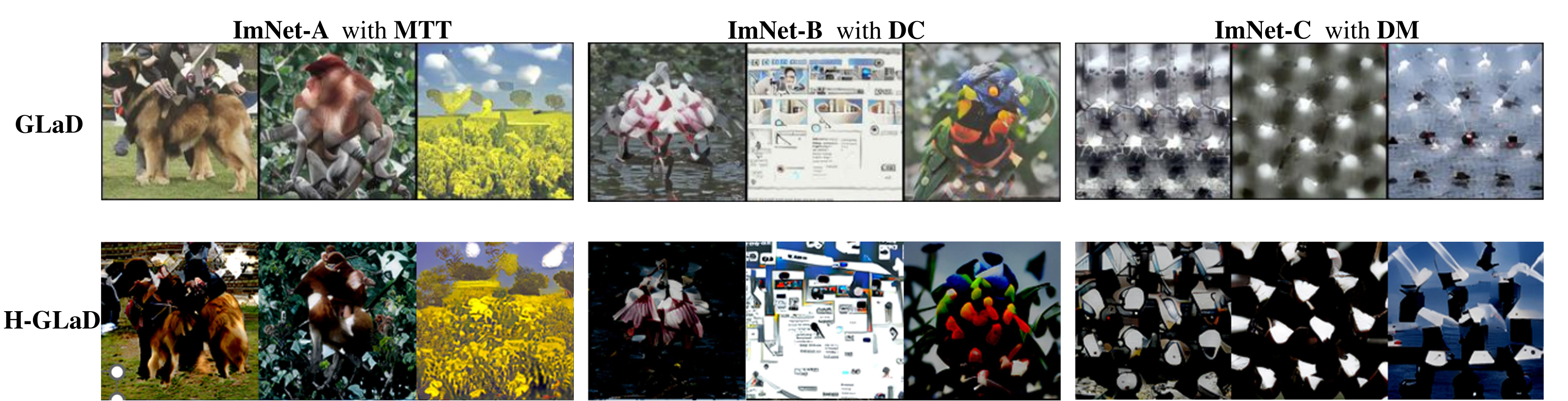
Figure 3: Visualization comparison of the synthetic datasets with different distillation methods.

4.3 Performance Improvements

The performance comparison of our method and previous works in MTT, DC, and DM is shown in Table 2 and Table 3. We report the same-architecture performance of the synthetic dataset with one image per class obtained using ConvNet-5 as the backbone network. Furthermore, we assess the performance of the synthetic dataset across different architectures. The cross-architecture accuracy is calculated by averaging the performance of the remaining four models, excluding the backbone model. The results of previous studies are acquired directly from the original papers. It can be observed that our method achieves consistent and significant improvements in MTT, DC, and DM methods compared to optimizing only in a fixed feature space. This indicates that our method successfully leverages the guidance information provided by all feature domains.

The cross-architecture performance on CIFAR-10 [14] is shown in Table 5. The results demonstrate that using a shallower StyleGAN-XL structure on the lower-resolution dataset CIFAR-10, H-GLaD still improves the performance of synthetic datasets distilled by different distillation methods. Please note that the released code of GLaD does not include the data augmentation and hyperparameter settings used by MTT on CIFAR10, which leads to a poor performance on ConvNet.

To align the proposed H-GLaD with GLaD on higher IPC, i.e. only $\text{IPC}=10$ under DC and DM is reported from original paper, our current confirmatory trials achieves a performance improvement of 1% to 3% compared to GLaD with $\text{IPC}=10$ under DC and DM as shown in Table 5, respectively, which demonstrates the effectiveness of H-GLaD.

As aforementioned, existing methods for GAN-based synthetic dataset parameterization encounter challenges in incomplete optimization and aligning optimal spaces across various settings. To address these issues, the proposed H-GLaD provides a straightforward yet effective method. Notably, H-GLaD consistently enhances or maintains high cross-architecture performance across various settings, reaffirming the effectiveness of the proposed method. The visualized images of synthetic datasets are depicted in Figure 3. Please refer to Appendix D for more visualization and Appendix B.4 for more corresponding qualitative interpretation.

Table 6: Ablation study of each component with different distillation method across various ImageNet-Subset under IPC=1.

Commponent	ImNet-B	ImNet-C	ImWoof	ImNet-Birds	ImNet-Fruits
GLaD-MTT	51.9$\pm 1.3$	44.9$\pm 0.4$	23.4$\pm 1.1$	35.8$\pm 1.4$	23.1$\pm 0.4$
+ Average Initialization	53.5$\pm 0.7$	46.1$\pm 0.9$	24.8$\pm 1.1$	36.5$\pm 0.8$	22.7$\pm 1.2$$\downarrow$
+ Hierarchical Layers	56.2$\pm 0.7$	48.1$\pm 0.9$	28.1$\pm 1.0$	38.5$\pm 1.2$	24.1$\pm 0.5$
+ Distance Metric	57.4$\pm 0.3$	49.5$\pm 0.6$	28.3$\pm 0.2$	39.7$\pm 0.8$	25.6$\pm 0.7$
GLaD-DC	49.2$\pm 1.1$	42.0$\pm 0.6$	22.3$\pm 1.1$	33.8$\pm 0.9$	20.7$\pm 1.1$
+ Average Initialization	48.9$\pm 0.8$$\downarrow$	40.6$\pm 0.7$$\downarrow$	22.8$\pm 1.4$	31.9$\pm 1.1$$\downarrow$	21.3$\pm 1.0$
+ Hierarchical Layers	50.1$\pm 1.1$	43.1$\pm 1.4$	23.6$\pm 0.8$	34.5$\pm 0.4$	21.9$\pm 0.8$
+ Distance Metric	50.7$\pm 0.9$	43.9$\pm 0.7$	24.0$\pm 0.8$	35.3$\pm 1.0$	22.4$\pm 1.1$
GLaD-DM	42.9$\pm 1.9$	39.4$\pm 1.7$	21.2$\pm 1.5$	27.6$\pm 1.9$	21.8$\pm 1.8$
+ Average Initialization	43.2$\pm 1.6$	39.9$\pm 1.7$	21.1$\pm 1.9$$\downarrow$	28.2$\pm 1.4$	22.3$\pm 1.3$
+ Hierarchical Layers	44.2$\pm 2.1$	41.0$\pm 1.2$	23.1$\pm 0.9$	29.0$\pm 1.5$	24.1$\pm 1.4$
+ Distance Metric	44.7$\pm 1.3$	41.1$\pm 1.3$	23.9$\pm 1.9$	29.5$\pm 1.5$	24.4$\pm 2.1$

4.4 Ablation Studies

Effectiveness of Each Component

As Table 6 shows, the two major components of our method, i.e., hierarchical feature domains (Sec. 3.2) and class-relevant feature distance (Sec. 3.3) both improve the performance across various ImageNet-Subsets with all distillation methods, especially on MTT. Optimizing in an unfixed feature space can bring significant gains, and on this basis, using class-relevant feature distance for implicit evaluation can yield a slight additional improvement. Please note that using class-relevant feature distance is infeasible without unfixed optimization spaces. Another secondary component, i.e., Initialization with averaged noise (Sec. 3.3) improves the performance of MTT and DM to some degree. However, it cannot achieve stable improvement in the performance of the DC method. We attribute this discrepancy to the inherent inclination towards noise and edge samples in DC.

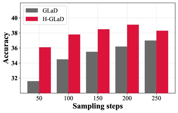
Figure 4: The comparison of performance(%) at the same optimization epoch.

Table 7: Ablation results of optimization steps per optimization space averaged on ImageNet-[A, B, C, D, E].

Steps MTT DC DM 20 46.9$\pm 1.2$ 39.8$\pm 1.1$ 39.1$\pm 1.2$ 50 47.2$\pm 0.8$ 41.6$\pm 0.8$ 37.0$\pm 1.7$ 100 50.3$\pm 0.6$ 43.2$\pm 0.6$ 6.5$\pm 1.4$ 200 50.5$\pm 0.4$ 43.0$\pm 0.6$ 35.8$\pm 1.1$

Optimization Steps

We perform 100 optimization steps in each layer to align with the sampling method in previous works. We conduct more experiments across different optimization steps to explore the correct optimization steps. By observing the results shown in Table 7, we find that optimization steps beyond 100 do not yield significant performance improvements for MTT and DC methods. Meanwhile, optimization steps below 100 result in performance degradation. Considering the trade-off between effects and costs, we set the steps at 100 for both MTT and DC. For DM, however, optimal performance is attained at the least number of steps per layer, i.e., 20 steps. To investigate whether the performance improvement is caused by the increasing sampling steps, We compare the performance of GLaD and H-GLaD at the same epoch. The results are shown in Figure 4, our method outperforms and converges faster, demonstrating the superiority of the approach in utilizing the hierarchical features.

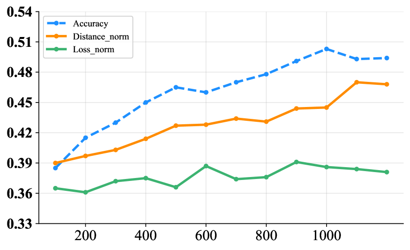
(a) Distillation Method: MTT

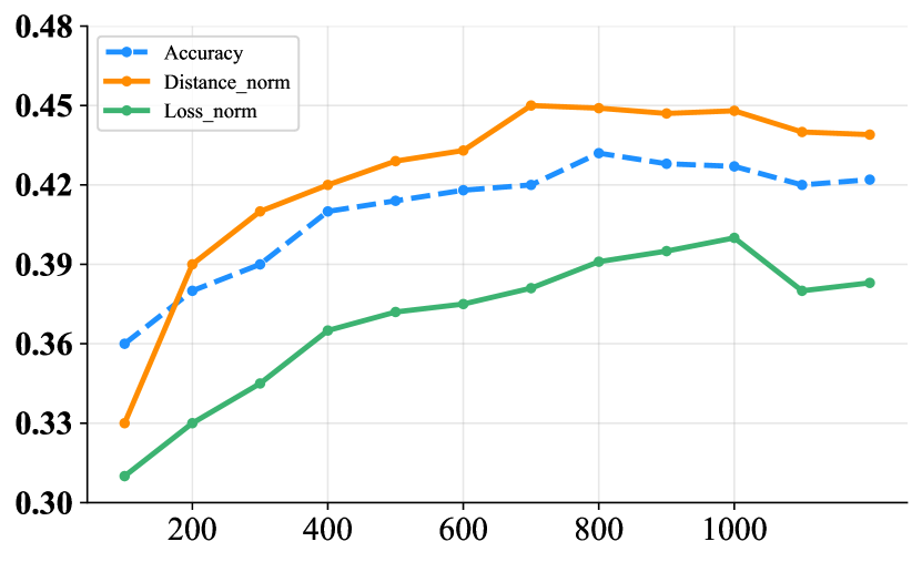
(b) Distillation Method: DC

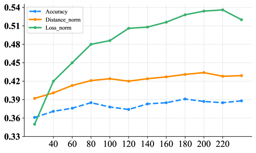
(c) Distillation Method: DM

Figure 5: The relationship between searching basis and performance. Note that higher loss-norm values indicate lower loss values and the same applies to feature distances.

Searching Basis

To avoid the time-consuming task of directly evaluating the synthetic dataset, we opt for class-relevant feature distance instead of the loss value for implicit searching. Specifically, we evaluate the synthetic dataset at specific epochs during the optimization process and subsequently record its ground-truth performance, loss value, and feature distance. Figure 5 demonstrates the recorded values during the optimization process. We normalize the values of loss function and feature distance to range $[0,1]$ for clear clarity and comparison. Our observation indicates that compared with the loss value, the feature distance consistently exhibits a stronger negative correlation with the real performance, proving the correctness of the designed distance metric.

Note that the objective of the proposed method is to improve the efficiency of utilizing informative guidance from various feature domains that have been overlooked in existing parameterization methods. Thus we treat the class-relevant distance merely as an evaluation criterion rather than an optimization target, avoiding the benefits derived from this distance.

5 Conclusion

In this paper, we present a novel approach to dataset distillation by leveraging hierarchical features within GAN models. Our method transforms the optimization space from a specific GAN feature domain to a broader feature space, addressing challenges seen in previous GAN-based dataset distillation methods. An advantage is that our approach outperforms existing methods in both same-architecture and cross-architecture scenarios. Additionally, we anticipate that further improvements can be achieved through detailed optimization steps and strategic feature layer combinations. This exploration of hierarchical features in GAN priors contributes to an advanced understanding of dataset distillation, paving the way for future research in optimizing synthetic datasets for diverse model architectures.

Appendix A Literature Reviews on Dataset Distillation

A.1 Dataset Distillation in Pixel Space

In this section, we review the methodology of optimizing synthetic dataset $S$ with the surrogate objective in pixel space, which provides the basic optimization objective for all parameterization dataset distillation methods.

DC [7].

Dataset Distillation (DD) [6] aims at optimizing the synthetic dataset $\mathcal{S}$ with a bi-level optimization. The main idea of bi-level optimization is that a network with parameter $\theta_{\mathcal{S}}$, which is trained on $\mathcal{S}$, should minimize the risk of the real dataset $\mathcal{T}$. However, due to the need to pass through an unrolled computation graph, DD brings about a significant amount of time overhead. Based on this, DC introduces a surrogate objective, which aims at matching the gradients of a network during the optimization. For a network with parameters $\theta_{S}$ trained on the synthetic data for some number of iterations, the matching loss is

$$\mathcal{L}_{\mathrm{DC}}=1-\frac{\nabla_{\theta}\ell^{\mathcal{S}}(\theta)\cdot\nabla_{\theta}\ell^{\mathcal{T}}(\theta)}{\left\|\nabla_{\theta}\ell^{\mathcal{S}}(\theta)\right\|\left\|\nabla_{\theta}\ell^{\mathcal{T}}(\theta)\right\|},$$ (6)

where $\ell^{\mathcal{T}}(\cdot)$ represents the loss function (e.g., CE loss) calculated on real dataset $\mathcal{T}$, and $\ell^{\mathcal{S}}(\cdot)$ is the same loss function calculated on synthetic dataset $\mathcal{T}$.

DM [9].

Despite DC significantly reducing time consumption through surrogate, bi-level optimization still introduces a substantial amount of time overhead, especially when dealing with high-resolution and large-scale datasets. DM achieves this by using only the features extracted from networks $\psi$ with random initialization as the matching target, the matching loss is

$$\mathcal{L}_{\mathrm{DM}}=\sum_{c}\left\|\frac{1}{\left|\mathcal{T}_{c}\right|}\sum_{\mathbf{x}\in\mathcal{T}_{c}}\psi(\mathbf{x})-\frac{1}{\left|\mathcal{S}_{c}\right|}\sum_{\mathbf{s}\in\mathcal{S}_{c}}\psi(\mathbf{s})\right\|^{2},$$ (7)

where $\mathcal{T}_{c}$ and $\mathcal{S}_{c}$ represents the real and synthetic images from class $c$ respectively.

MTT [8].

Distinct from the short-range optimization introduced from DC, MTT utilizes many expert trajectories $\{\theta^{*}_{t}\}^{T}_{0}$ which are obtained by training networks from scratch on the full real dataset and choose the parameter distance the matching objective. During the distillation process, a student network is initialized with parameters $\theta^{*}_{t}$ by sample expert trajectory at timestamp $t$ and then trained on the synthetic data for some number of iterations $N$, the matching loss is

$$\mathcal{L}_{\mathrm{MTT}}=\frac{\left\|\hat{\theta}_{t+N}-\theta_{t+M}^{*}\right\|^{2}}{\left\|\theta_{t}^{*}-\theta_{t+M}^{*}\right\|^{2}},$$ (8)

where $\theta_{t+M}^{*}$ represents the expert trajectory at timestamp $t+M$.

A.2 Dataset Distillation in Feature Domain

In this section, we review the methodology of parameterization dataset distillation built upon the aforementioned dataset distillation methods, achieving better performance by employing a differentiable operation $\mathcal{F}(\cdot)$ to shift the optimization space from pixel space to various feature domain, which can be formulated as

$$\mathcal{S}=\{\mathcal{F}(\mathbf{z})\}.$$ (9)

where $\mathbf{z}$ represents latent code in the feature domain corresponding to $\mathcal{F}(\cdot)$.

HaBa [11].

HaBa breaks the synthetic dataset into bases and a small neural network called hallucinator which is utilized to produce additional synthetic images. By leveraging this technique, the resulting model could be regarded as a differentiable operation and produce more diverse samples. However, HaBa simultaneously optimizes the bases and the hallucinator, neglecting the relationship between the two feature domains. This leads to unstable optimization during the training process.

IDC [26].

IDC proposes a principle that small-sized synthetic images often carry more effective information under the same spatial budget and utilize an upsampling module as the differentiable operation. Despite employing a differentiable operation, the optimization of IDC is still the pixel space, which resulted in the loss of effective information gain obtained from other feature domains.

FreD [13].

FreD suggests that optimizing for the main subject in the synthetic image is more instructive than optimizing for all the details. Therefore, FreD employs discrete cosine transform (DCT) as the differentiable operation and uses a learnable mask matrix to remove high-frequency information, ensuring that the optimization process only occurs in the low-frequency domain. This allows the synthetic dataset to achieve higher performance and generalization. However, FreD overlooks the effective guiding information within the high-frequency domain and fails to connect the two feature domains produced by DCT, leading to potential incomplete optimization.

GLaD [12].

GLaD employs a pre-trained generative model (i.e., GAN) and distills the synthetic dataset in the latent space of the generative model. By leveraging the capability of a generative model to map latent noise to image patterns, GLaD achieves better generalization to unseen architecture and scale to high-dimensional datasets. However, for StyleGAN, the earlier layers tend to provide the information about the main subject in an image while the later layers often contribute to the details. However, GLaD attempts to balance the low-frequency information with the high-frequency information by selecting an intermediate layer as a fixed optimization space, discarding the guiding information from the earlier layers can lead to incomplete optimization. Another limitation of GLaD is the need for a large number of preliminary experiments. GLaD selects a specific intermediate layer suitable for all datasets for different distillation methods, However, under the same distillation method, the optimal intermediate layer corresponding to different datasets is not the same, especially when the manifold of the datasets varies greatly, which suggests that GLaD cannot spontaneously adapt to different datasets, distillation methods, and GANs.

Appendix B Additional Experimental Results

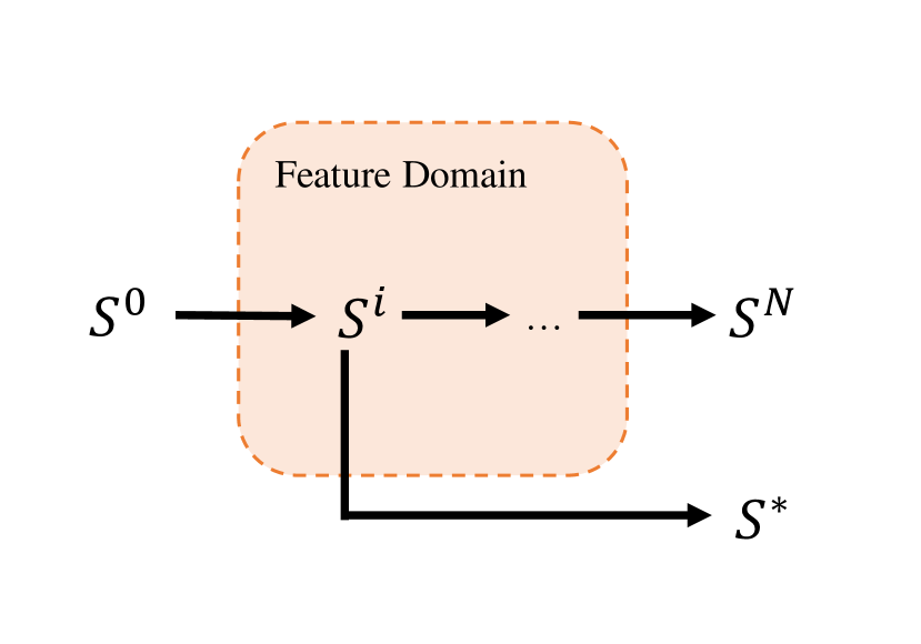
(a) Fixed optimization space

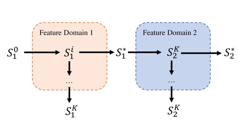
(b) Unfixed optimization space

Figure 6: The comparison between fixed optimization space and unfixed optimization space. $\mathcal{S}^{i}$ is the synthetic dataset at optimization steps $i$, $\mathcal{S}^{*}$ is the optimal synthetic dataset selected during the optimization path, $\mathcal{S}_{j}$ is the synthetic dataset optimized in feature domain $j$.

B.1 Unfixed Optimization Space vs Fixed Optimization Space

Figure 6 demonstrates the optimization processes of fixed space and unfixed space. As shown in Figure 6, Besides the lack of informative guidance in multiple feature domains, the fixed optimization space has another severe limitation that prevents further optimization by leveraging synthetic dataset that perform better through implicit or explicit selection. The optimization process within a fixed feature domain can be considered a continuous process. Assuming that a temporarily optimal result is selected within a segment of the optimization path before convergence, and the number of optimization epochs corresponding to this result is not the end of this optimization path, the optimization process then faces a dilemma: whether to use the selected optimal result as the starting point for the next segment of the optimization path, or to abandon the use of this optimal result. Choosing the latter may lead the optimization process to fall into a local optimum due to the lack of effective guidance, while choosing the former may result in a cycle of optimization, which means the optimization process have to abandon remaining optimization results and restart.

Table 8: Abltion study on optimization space comparison. "Fixed (Pixel)" refers to optimize in pixel space and "Fixed (GAN)" refers to GLaD, while Unfixed refers to optimize in multiple feature domains.

Alg.	Opimization Space	ImNet-A	ImNet-B	ImNet-C	ImNet-D	ImNet-E	ImNette	ImWoof	ImNet-Birds	ImNet-Fruits	ImNet-Cats
	Fixed (Pixel)	51.7$\pm 0.2$	53.3$\pm 1.0$	48.0$\pm 0.7$	43.0$\pm 0.6$	39.5$\pm 0.9$	41.8$\pm 0.6$	22.6$\pm 0.6$	37.3$\pm 0.8$	22.4$\pm 1.1$	22.6$\pm 0.4$
MTT	Fixed (GAN)	50.7$\pm 0.4$	51.9$\pm 1.3$	44.9$\pm 0.4$	39.9$\pm 1.7$	37.6$\pm 0.7$	38.7$\pm 1.6$	23.4$\pm 1.1$	35.8$\pm 1.4$	23.1$\pm 0.4$	26.0$\pm 1.1$
	Unfixed	53.1$\pm 0.8$	55.4$\pm 0.7$	47.5$\pm 0.9$	44.1$\pm 0.6$	40.8$\pm 0.7$	42.8$\pm 1.0$	27.0$\pm 0.6$	37.6$\pm 0.9$	24.7$\pm 0.7$	28.3$\pm 0.8$
	Fixed (Pixel)	43.2$\pm 0.6$	47.2$\pm 0.7$	41.3$\pm 0.7$	34.3$\pm 1.5$	34.9$\pm 1.5$	34.2$\pm 1.7$	22.5$\pm 1.0$	32.0$\pm 1.5$	21.0$\pm 0.9$	22.0$\pm 0.6$
DC	Fixed (GAN)	44.1$\pm 2.4$	49.2$\pm 1.1$	42.0$\pm 0.6$	35.6$\pm 0.9$	35.8$\pm 0.9$	35.4$\pm 1.2$	22.3$\pm 1.1$	33.8$\pm 0.9$	20.7$\pm 1.1$	22.6$\pm 0.8$
	Unfixed	46.1$\pm 0.7$	50.0$\pm 0.9$	43.8$\pm 1.4$	37.1$\pm 0.9$	36.6$\pm 0.6$	36.2$\pm 0.5$	22.7$\pm 0.3$	34.9$\pm 1.5$	21.2$\pm 0.8$	23.1$\pm 0.3$
	Fixed (Pixel)	39.4$\pm 1.8$	40.9$\pm 1.7$	39.0$\pm 1.3$	30.8$\pm 0.9$	27.0$\pm 0.8$	30.4$\pm 2.7$	20.7$\pm 1.0$	26.6$\pm 2.6$	20.4$\pm 1.9$	20.1$\pm 1.2$
DM	Fixed (GAN)	41.0$\pm 1.5$	42.9$\pm 1.9$	39.4$\pm 1.7$	33.2$\pm 1.4$	30.3$\pm 1.3$	32.2$\pm 1.7$	21.2$\pm 1.5$	27.6$\pm 1.9$	21.8$\pm 1.8$	22.3$\pm 1.6$
	Unfixed	42.3$\pm 1.5$	44.1$\pm 1.5$	41.3$\pm 1.7$	33.7$\pm 1.1$	31.5$\pm 1.1$	34.0$\pm 1.2$	23.1$\pm 1.3$	28.9$\pm 1.4$	24.3$\pm 1.3$	22.8$\pm 0.8$

B.2 More Comparisons with GLaD

To expand the optimization space, the method we proposed utilizes hierarchical feature domains composed of intermediate layers from GAN. To investigate whether optimization across multiple feature domains is superior to optimization within a single fixed feature domain, we evaluate the performance by simply expanding the optimization space based on the baseline. As shown in Table 8, compared to GLaD, which only selects a single yet optimal intermediate layer of the GAN as the optimization space, H-GLaD has successfully achieved considerable improvement, validating our viewpoint that the optimization result from the previous feature domain can serve as better starting point for subsequent feature domain. Please note the result is obtained by not selecting $\mathcal{S}^{*}$.

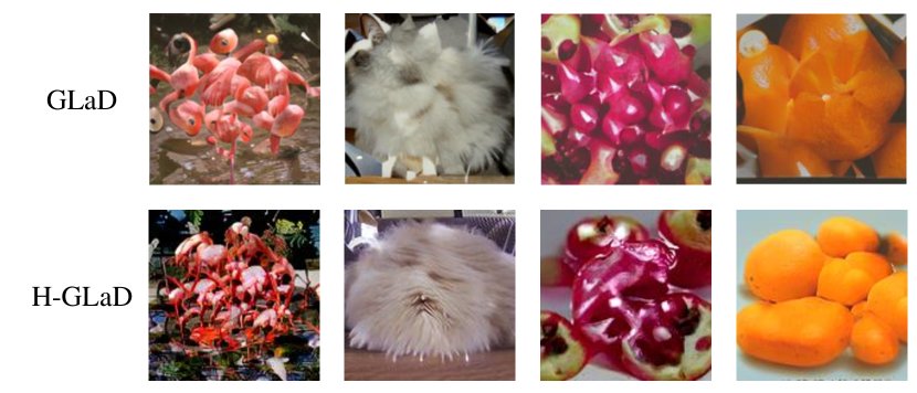
Figure 7: The comparison of visualization.

Table 9: Higher-resolution (256×256) synthetic dataset (using DC) cross-architecture performance (%).

Method ImNet-A ImNet-B ImNet-C ImNet-D ImNet-D Pixel 38.3$\pm 4.7$ 32.8$\pm 4.1$ 27.6$\pm 3.3$ 25.5$\pm 1.2$ 23.5$\pm 2.4$ GLaD 37.4$\pm 5.5$ 41.5$\pm 1.2$ 35.7$\pm 4.0$ 27.9$\pm 1.0$ 29.3$\pm 1.2$ H-GLaD 40.7$\pm 2.1$ 42.9$\pm 1.8$ 37.2$\pm 2.2$ 30.1$\pm 1.7$ 29.7$\pm 1.8$

To present a more comprehensive comparison, we evaluate the cross-architecture performance of a high-resolution synthetic dataset under the same setting (i.e., DC on ImageNet-[A, B, C, D, E] under IPC=1). As shown in Table 9, our proposed H-GLaD still achieves considerable improvements, demonstrating the stability of our proposed method. Figure 7 illustrates the comparison of synthetic dataset visualization generated by H-GLaD and GLaD using the same initial image. The images produced by H-GLaD achieve a good balance between content and style. On one hand, H-GLaD tends to preserve more main subject information by optimizing in the earlier layers of the GAN. On the other hand, since H-GLaD also undergoes optimization in the later layers, the synthetic images tend to be sharper and rarely produce the kaleidoscope-like patterns that are common in the GLaD method.

Table 10: Synthetic dataset performance(%) using MTT with StyleGAN-XL trained on different datasets.

Training Dataset	ImNet-A	ImNet-B	ImNet-C	ImNet-D	ImNet-E	ImNette	ImWoof	ImNet-Birds	ImNet-Fruits	ImNet-Cats
-	55.7$\pm 0.8$	55.2$\pm 0.7$	46.2$\pm 0.9$	43.1$\pm 0.6$	43.2$\pm 0.6$	43.7$\pm 0.7$	28.7$\pm 1.0$	38.1$\pm 1.2$	24.9$\pm 0.5$	30.1$\pm 0.4$
Pokemon	53.6$\pm 1.2$	56.9$\pm 0.5$	48.3$\pm 0.8$	44.4$\pm 0.7$	42.4$\pm 1.0$	44.9$\pm 0.6$	29.4$\pm 0.5$	38.6$\pm 0.9$	26.1$\pm 1.3$	38.7$\pm 1.0$
FFHQ	53.4$\pm 0.7$	57.8$\pm 0.8$	48.2$\pm 0.5$	46.0$\pm 0.6$	42.2$\pm 0.8$	44.4$\pm 0.3$	27.9$\pm 1.1$	39.9$\pm 0.6$	24.8$\pm 1.6$	28.9$\pm 0.7$
ImageNet-1k	55.1$\pm 0.6$	57.4$\pm 0.3$	49.5$\pm 0.6$	46.3$\pm 0.9$	43.0$\pm 0.6$	45.4$\pm 1.1$	28.3$\pm 0.2$	39.7$\pm 0.8$	25.6$\pm 0.7$	29.6$\pm 1.0$

B.3 Pre-trained Deep Generative Prior

In Table 10, we show the results obtained from both randomly initialized StyleGAN-XL [34] and StyleGAN-XL trained on various datasets using MTT under IPC=1. The results demonstrate that our approach can achieve comparable performance even when the GAN is not specifically trained on the relevant dataset, indicating the outstanding generalizability of H-GLaD.

Notably, with the observation that the StyleGAN-XL trained on ImageNet-1k tends to be more suitable for non-fine-grained classification problems, while the StyleGAN-XL trained on Pokemon or randomly initialized StyleGAN-XL often performs better on fine-grained classification problems. Indicating that our approach can not only effectively exploit the information of the relevant dataset across hierarchical feature domains within the GAN but is also capable of utilizing the underlying connection that exists after different datasets are mapped into the GAN feature domain. However, pre-trained StyleGAN-XL on FFHQ often leads to a decrease in performance, which also indicates from another aspect that there is a significant feature gap between facial data and real-world data (e.g., ImageNet-1k).

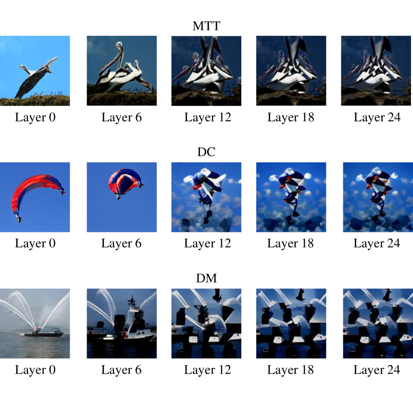
(a) Visualization of synthetic images.

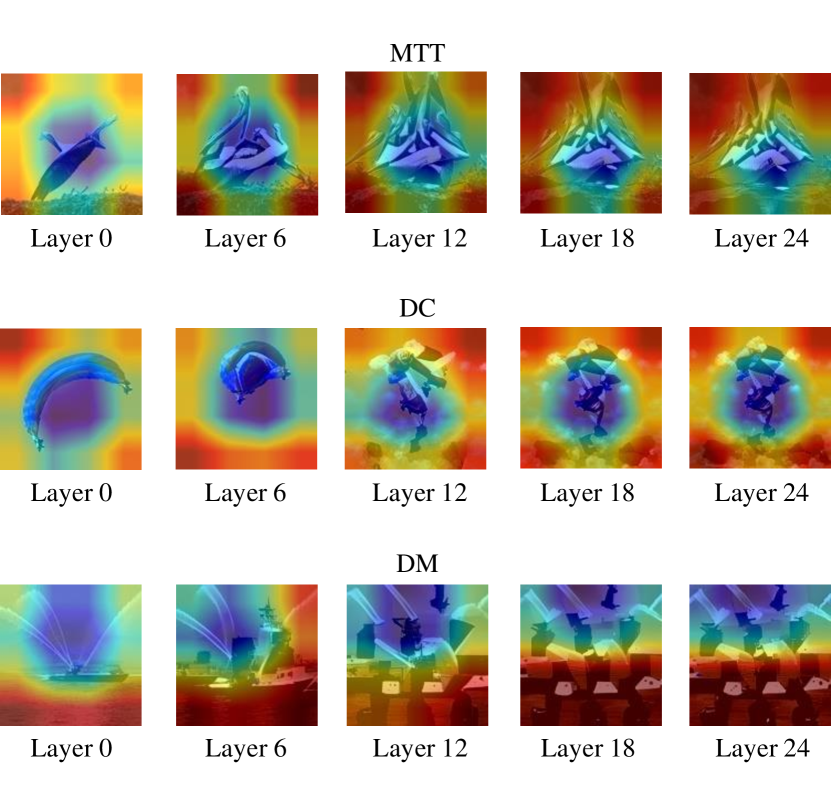
(b) Visualization of corresponding CAM.

Figure 8: The visualization change of synthetic images and corresponding CAM during the optimization process using different distillation methods. "Layer" refers to the index of intermediate layers provided by StyleGAN-XL.

B.4 Visualizing Morphological Transition of Synthetic Images

As shown in Figure 8(a), we demonstrate the visualization changes of the synthetic image throughout the optimization process. Layer $0$ represents the initial image produced by StyleGAN-XL using averaged noise, and Layer $i$ indicates the image when the optimization space reaches layer $i$. In the early stage of optimization, since the optimization space is located in the earlier layer of the GAN, the optimization object primarily focus on the main subject of the synthetic image. Meanwhile, GAN still maintains a high degree of integrity which leads to a strong constraint on the slight changes in the latent produced during the optimization process, which can be transformed into patterns resembling real images instead of noises. Thus the tendency in the early stage of optimization is to generate images that better conform to the constraint of distillation loss yet appear more realistic, leading to produce synthetic images that can be regarded as a better starting point for the subsequent optimization process.

In the later stage of optimization, the main subject of the synthetic image no longer undergoes significant changes, and the optimization objective shifts along with the movement of the optimization space, focusing more on the details of the synthetic images. As shown in Figure 8(a), due to the weakened generative constraint of the incomplete GAN, the final synthetic image becomes similar to the indistinguishable and distorted image produced by existing distillation methods. Building upon the better synthetic image obtained through the optimization process in the earlier layers, different distillation methods gradually incorporate more guidance-oriented customized patterns into the synthetic image, achieving further performance improvement.

B.5 Qualitative Interpretation using CAM

We additionally introduce CAM [39] to visualize the heatmap of class-relevant information in the synthetic images as shown in Figure 8(b), which also demonstrates our perspective from another aspect. The blue areas represent regions of class-relevant information, which can produce the largest gradient during the training process. Conversely, the red areas indicate regions of class-irrelevant information, with deeper colors signifying higher degrees of corresponding information. In the early stage of optimization, the class-relevant information of the main subject in the synthetic image produced by various distillation methods is compressed.

Interestingly, for the gradient matching methods MTT and DC, which rely on long-range and short-range gradient matching respectively, the class-relevant information of the main subject remains unchanged when optimization space changes to later layers, while the gradient that can be produced by the image background (e.g., corners) are further decreased, as indicated by the deeper red color, even though the changes in the background are hardly observable by the naked eye during the optimization process. However, for the feature matching method DM, compared to the visualized kaleidoscope-like pattern, the visualization of corresponding CAM shows an unbalanced distribution and focuses on areas not typically observed by humans. We believe this phenomenon also explains the poorer performance of DM compared with gradient matching methods. Compared to the synthetic images with a centralized concentration of class-relevant information produced by MTT and DC, the images generated by DM are too diverse due to fitting all the features of the entire dataset including the class-irrelevant features, which is disadvantageous for training neural networks on tiny distilled datasets.

Table 11: Abltion study on layers combination and optimization allocation using MTT. "Layers" refers to the number of layers per optimization space, "Optimization" refers to the number of SGD steps allocated in each optimization space.

Layers	Optimization	ImNet-A	ImNet-B	ImNet-C	ImNet-D	ImNet-E	ImNette	ImWoof	ImNet-Birds	ImNet-Fruits	ImNet-Cats
	50	53.6$\pm 0.2$	55.2$\pm 1.5$	47.3$\pm 0.5$	44.1$\pm 0.7$	40.5$\pm 1.1$	43.8$\pm 0.4$	26.6$\pm 0.7$	37.1$\pm 0.6$	22.9$\pm 0.5$	27.8$\pm 1.0$
1	100	55.3$\pm 0.8$	57.1$\pm 0.7$	49.1$\pm 0.9$	46.6$\pm 0.4$	42.2$\pm 1.5$	44.9$\pm 1.2$	28.6$\pm 0.6$	39.4$\pm 0.8$	25.9$\pm 0.7$	30.1$\pm 1.2$
	200	55.4$\pm 0.7$	57.5$\pm 1.1$	48.6$\pm 0.8$	46.2$\pm 0.9$	43.6$\pm 0.6$	45.7$\pm 0.5$	28.7$\pm 0.4$	39.4$\pm 0.6$	25.5$\pm 0.5$	29.8$\pm 0.2$
	50	51.3$\pm 0.9$	54.2$\pm 1.1$	46.3$\pm 0.8$	44.1$\pm 1.2$	40.3$\pm 1.2$	41.8$\pm 1.4$	27.1$\pm 0.6$	36.5$\pm 1.1$	23.0$\pm 1.2$	28.1$\pm 1.3$
2	100	55.1$\pm 0.6$	57.4$\pm 0.3$	49.5$\pm 0.6$	46.3$\pm 0.9$	43.0$\pm 0.6$	45.4$\pm 1.1$	28.3$\pm 0.2$	39.7$\pm 0.8$	25.6$\pm 0.7$	29.6$\pm 1.0$
	200	55.6$\pm 0.9$	57.9$\pm 0.5$	49.4$\pm 0.3$	46.0$\pm 0.1$	43.5$\pm 0.4$	45.1$\pm 0.7$	28.6$\pm 0.2$	39.3$\pm 0.8$	25.9$\pm 1.1$	29.9$\pm 0.6$
	50	51.8$\pm 0.7$	52.9$\pm 1.2$	46.1$\pm 1.5$	42.3$\pm 0.5$	39.8$\pm 0.5$	40.9$\pm 1.3$	24.7$\pm 1.1$	35.9$\pm 0.5$	21.2$\pm 1.7$	25.3$\pm 1.1$
4	100	53.3$\pm 0.8$	54.2$\pm 1.1$	47.3$\pm 1.2$	41.8$\pm 1.7$	42.7$\pm 0.6$	27.7$\pm 0.5$	27.1$\pm 1.0$	27.0$\pm 0.9$	22.5$\pm 1.4$	26.4$\pm 1.2$
	200	55.0$\pm 1.0$	57.0$\pm 1.3$	48.1$\pm 1.6$	45.2$\pm 0.5$	42.1$\pm 1.4$	45.0$\pm 0.5$	27.2$\pm 0.9$	38.8$\pm 1.1$	24.6$\pm 0.5$	28.4$\pm 0.8$

Table 12: Abltion study on layers combination and optimization allocation using DC.

Layers	Optimization	ImNet-A	ImNet-B	ImNet-C	ImNet-D	ImNet-E	ImNette	ImWoof	ImNet-Birds	ImNet-Fruits	ImNet-Cats
	50	45.2$\pm 1.2$	48.3$\pm 1.3$	42.0$\pm 0.4$	36.2$\pm 0.7$	35.0$\pm 0.8$	35.8$\pm 1.1$	22.7$\pm 1.0$	33.5$\pm 0.5$	21.1$\pm 1.5$	22.7$\pm 0.8$
1	100	46.2$\pm 0.7$	51.1$\pm 0.4$	43.3$\pm 1,1$	37.2$\pm 0.5$	36.6$\pm 0.9$	36.7$\pm 1.3$	22.9$\pm 0.8$	35.6$\pm 1.1$	22.1$\pm 1.5$	23.8$\pm 0.7$
	200	46.5$\pm 0.9$	50.7$\pm 1.1$	43.8$\pm 0.2$	37.3$\pm 0.7$	37.6$\pm 0.7$	36.9$\pm 1.3$	24.3$\pm 0.5$	34.9$\pm 0.3$	22.6$\pm 1.3$	23.6$\pm 0.7$
	50	44.8$\pm 0.4$	48.9$\pm 0.9$	42.1$\pm 1.1$	35.6$\pm 1.0$	36.6$\pm 0.6$	34.2$\pm 1.1$	22.1$\pm 0.6$	33.3$\pm 1.6$	20.0$\pm 1.3$	22.7$\pm 0.8$
2	100	46.9$\pm 0.8$	50.7$\pm 0.9$	43.9$\pm 0.7$	37.4$\pm 0.4$	37.2$\pm 0.3$	36.9$\pm 0.8$	24.0$\pm 0.8$	35.3$\pm 1.0$	22.4$\pm 1.1$	24.1$\pm 0.9$
	200	46.8$\pm 0.5$	50.8$\pm 0.3$	43.4$\pm 0.6$	37.0$\pm 1.3$	37.3$\pm 0.5$	37.1$\pm 0.7$	23.8$\pm 1.3$	35.6$\pm 1.1$	22.1$\pm 1.2$	24.6$\pm 1.3$
	50	43.6$\pm 0.7$	47.8$\pm 0.7$	40.4$\pm 0.6$	34.6$\pm 0.5$	34.2$\pm 0.8$	33.4$\pm 1.2$	21.3$\pm 0.9$	32.7$\pm 1.4$	19.9$\pm 0.5$	21.6$\pm 0.6$
4	100	45.7$\pm 0.7$	49.4$\pm 0.9$	43.1$\pm 1.1$	36.1$\pm 1.3$	36.4$\pm 0.8$	35.2$\pm 0.6$	23.4$\pm 1.1$	34.7$\pm 0.5$	21.3$\pm 1.1$	23.5$\pm 1.3$
	200	46.3$\pm 0.8$	50.1$\pm 0.9$	43.2$\pm 0.7$	37.0$\pm 0.4$	36.8$\pm 1,6$	36.2$\pm 1.0$	23.3$\pm 1.3$	34.4$\pm 1.4$	21.6$\pm 0.8$	23.7$\pm 0.5$

B.6 Layers Combination and Optimization Allocation

As discussed in Section 4.2, we adopt a uniform sampling method that evaluates the synthetic dataset per $100$ optimization epochs (even less when using DM) to align with the evaluation method of the baseline (i.e., GLaD). Additionally, we decompose StylGAN-XL into $G_{11}\circ\cdots\circ G_{1}\circ G_{0}(\,\cdot\,)$ to align with the time complexity of the baseline. In Section 4.4, we present an ablation study on the allocation of optimization epochs per optimization space. Building on this, we further explore the impact of combining different numbers of intermediate layers into a single optimization space and allocating different numbers of optimization epochs to each optimization space on the performance of the synthetic dataset. For all distillation methods, we explore the impact of varying optimization spaces by using combinations of $1$, $2$, and $4$ intermediate layers within each optimization space. Under the same optimization space setting, for MTT and DC, we investigated the effects of different numbers of optimization epochs allocated to each optimization space by using $50$, $100$, and $200$. For DM, due to the overfitting issue caused by feature matching, we used $10$, $20$, and $50$ as the number of optimization epochs per optimization space.

The results for MTT and DC are shown in Table 11 and Table 12. Combining $1$ or $2$ intermediate layers as a single optimization space does not produce a significant impact on the performance, indicating that existing redundant feature spaces provided by GAN contribute little to the distillation tasks and may even lead to a negative effect. Under this setting, allocating $50$ optimization epochs per optimization space produces a clear phenomenon of optimization not converging. However, when the number of optimization epochs comes to $100$ or $200$, the optimization converges without significant performance differences. Achieved by implicitly selecting the optimal synthetic dataset through the proposed class-relevant feature distance metric, allowing us to avoid overfitting issues to some extent through a certain level of optimization path withdrawal. Therefore, we choose $100$ epochs as the basic setting to reduce time complexity in the actual training process. When using $4$ intermediate layers as an optimization space, the performance is decreased even when setting optimization epochs to $200$, indicating that too few feature domains could not provide sufficiently rich guiding information, forcing the optimization process to require more epochs to converge, demonstrating the superiority of our proposed H-GLaD in utilizing multiple feature domains.

Table 13: Abltion study on layers combination and optimization allocation using DM.

Layers	Optimization	ImNet-A	ImNet-B	ImNet-C	ImNet-D	ImNet-E	ImNette	ImWoof	ImNet-Birds	ImNet-Fruits	ImNet-Cats
	10	42.1$\pm 2.2$	44.1$\pm 1.6$	41.7$\pm 1.7$	33.9$\pm 1.2$	31.3$\pm 1.9$	34.2$\pm 2.1$	24.1$\pm 1.4$	29.7$\pm 0.7$	24.1$\pm 1.6$	22.6$\pm 1.3$
1	20	41.6$\pm 1.6$	44.8$\pm 1.8$	41.3$\pm 1.4$	34.1$\pm 2.1$	31.2$\pm 0.5$	33.7$\pm 0.6$	24.0$\pm 1.3$	29.6$\pm 1.7$	23.4$\pm 0.8$	23.7$\pm 1.9$
	50	40.2$\pm 1.6$	43.4$\pm 1.7$	40.2$\pm 2.0$	33.1$\pm 1.3$	29.7$\pm 1.8$	32.6$\pm 1.9$	23.1$\pm 2.1$	28.2$\pm 1.6$	22.1$\pm 0.8$	21.0$\pm 0.5$
	10	41.4$\pm 1.7$	43.5$\pm 1.3$	40.4$\pm 0.9$	34.1$\pm 1.3$	31.3$\pm 1.8$	33.6$\pm 1.7$	22.4$\pm 1.6$	28.3$\pm 2.1$	23.1$\pm 1.7$	22.9$\pm 1.5$
2	20	42.8$\pm 1.2$	44.7$\pm 1.3$	41.1$\pm 1.3$	34.8$\pm 1.5$	31.9$\pm 0.9$	34.8$\pm 1.0$	23.9$\pm 1.9$	29.5$\pm 1.5$	24.4$\pm 2.1$	24.2$\pm 1.1$
	50	40.1$\pm 1.8$	42.6$\pm 2.0$	40.2$\pm 1.6$	32.6$\pm 1.7$	29.7$\pm 1.3$	33.1$\pm 0.6$	21.6$\pm 0.7$	27.7$\pm 1.6$	22.2$\pm 1.3$	22.4$\pm 1.9$
	10	39.9$\pm 1.4$	42.5$\pm 1.0$	40.4$\pm 1.8$	32.4$\pm 1.6$	30.1$\pm 2.4$	32.7$\pm 2.3$	20.9$\pm 1.6$	27.5$\pm 2.2$	22.5$\pm 1.7$	21.8$\pm 1.2$
4	20	40.6$\pm 1.3$	42.5$\pm 1.6$	39.6$\pm 2.1$	32.2$\pm 1.5$	30.1$\pm 1.3$	32.9$\pm 1.8$	21.6$\pm 1.5$	27.3$\pm 1.2$	21.7$\pm 2.3$	22.3$\pm 1.6$
	50	40.4$\pm 1.7$	42.7$\pm 1.3$	39.9$\pm 1.2$	32.0$\pm 1.4$	30.3$\pm 1.9$	32.6$\pm 1.6$	22.0$\pm 1.1$	27.8$\pm 0.9$	21.1$\pm 1.7$	22.6$\pm 1.4$

The results for DM are shown in Table 13. Similar to MTT and DC, Combining $1$ or $2$ intermediate layers as a single optimization space results in similar performance, while combining $4$ intermediate layers as optimization space leads to a significant performance drop. However, under the same optimization space settings, an excessive number of optimization epochs often leads to a severe decline in performance when using DM as the distillation method. As aforementioned, DM is unable to focus on class-relevant information, which causes an irreversible loss of the main subject information in the synthetic image after deploying a large number of optimization epochs in a specific feature domain, which in turn leads to a situation where the informative guidance provided by subsequent feature domains could not be effectively incorporated into the synthetic image, resulting in performance degradation. In this case, even the proposed class-relevant feature distance could not effectively select a superior synthetic dataset. To align with the approach of decomposing GAN used in MTT and DC, we ultimately combine $2$ intermediate layers as an optimization space and deploy 20 optimization epochs as the experimental setting for DM.

Table 14: Quantitative results on searching basis. "-" refers to not employing a searching strategy, "Loss Value" refers to directly using corresponding loss function value as the searching basis, "Feature Distance" refers to the use of proposed class-relevant distance as a searching basis

Alg.	Searching Basis	ImNet-A	ImNet-B	ImNet-C	ImNet-D	ImNet-E	ImNette	ImWoof	ImNet-Birds	ImNet-Fruits	ImNet-Cats
	-	54.7$\pm 0.8$	56.2$\pm 0.7$	48.1$\pm 0.9$	45.4$\pm 0.9$	41.8$\pm 0.6$	43.8$\pm 0.8$	28.1$\pm 1.0$	38.5$\pm 1.2$	24.1$\pm 0.5$	28.7$\pm 0.9$
MTT	Loss Value	53.6$\pm 0.9$	56.9$\pm 0.7$	48.3$\pm 0.8$	45.0$\pm 0.6$	41.0$\pm 1.2$	44.5$\pm 0.8$	27.5$\pm 1.4$	37.8$\pm 0.7$	25.1$\pm 0.9$	27.6$\pm 1.0$
	Feature Distance	55.1$\pm 0.6$	57.4$\pm 0.3$	49.5$\pm 0.6$	46.3$\pm 0.9$	43.0$\pm 0.6$	45.4$\pm 1.1$	28.3$\pm 0.2$	39.7$\pm 0.8$	25.6$\pm 0.7$	29.6$\pm 1.0$
	-	45.9$\pm 0.7$	50.1$\pm 1.1$	43.1$\pm 1.4$	36.9$\pm 0.8$	36.8$\pm 0.6$	36.0$\pm 0.9$	23.6$\pm 0.8$	34.5$\pm 0.4$	21.9$\pm 0.8$	23.2$\pm 0.9$
DC	Loss Value	46.6$\pm 1.3$	48.9$\pm 1.7$	43.6$\pm 1.1$	36.1$\pm 1.2$	36.6$\pm 0.5$	36.2$\pm 0.9$	23.1$\pm 0.6$	33.6$\pm 0.7$	21.3$\pm 1.1$	22.8$\pm 1.0$
	Feature Distance	46.9$\pm 0.8$	50.7$\pm 0.9$	43.9$\pm 0.7$	37.4$\pm 0.4$	37.2$\pm 0.3$	36.9$\pm 0.8$	24.0$\pm 0.8$	35.3$\pm 1.0$	22.4$\pm 1.1$	24.1$\pm 0.9$
	-	42.4$\pm 1.6$	44.2$\pm 2.1$	41.0$\pm 1.2$	34.0$\pm 1.2$	31.1$\pm 1.0$	34.5$\pm 2.1$	23.1$\pm 0.9$	29.0$\pm 1.5$	24.1$\pm 1.4$	22.6$\pm 1.5$
DM	Loss Value	41.6$\pm 1.8$	44.4$\pm 1.4$	40.7$\pm 2.1$	34.6$\pm 1.7$	30.1$\pm 1.3$	34.5$\pm 1.3$	23.6$\pm 1.2$	28.7$\pm 1.3$	24.4$\pm 1.3$	21.2$\pm 1.2$
	Feature Distance	42.8$\pm 1.2$	44.7$\pm 1.3$	41.1$\pm 1.3$	34.8$\pm 1.5$	31.9$\pm 0.9$	34.8$\pm 1.0$	23.9$\pm 1.9$	29.5$\pm 1.5$	24.4$\pm 2.1$	24.2$\pm 1.1$

B.7 Ablation Study on Searching Strategy

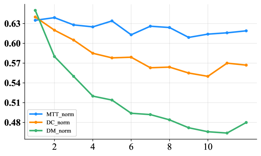
Figure 9: Quantitative results of loss function value using different distillation methods. Note that we normalize all the values for clear comparison.

To better utilize the informative guidance provided by multiple feature domains, we propose class-relevant feature distance as an evaluation metric for implicitly selecting the optimal synthetic dataset. We demonstrate the ablation study using different implicit evaluation metrics, as shown in Table 14, the metric we proposed outperforms the use of loss function value corresponding to the distillation methods as the metric under all settings. It is worth noting that, although the accuracy of the model trained on the synthetic dataset can be used as an explicit evaluation metric for the data distillation task, the evaluation process incurred much greater time overhead than the distillation task itself, rendering it impractical for actual training processes.

To explore the principle of the superiority of class-relevant feature distance, we first discussed the respective limitations of directly using existing distillation loss function value as the evaluation metric. The tendency of different distillation loss functions is shown in Figure 9. For MTT, the loss function is obtained by calculating the distance between the student network parameters and the teacher network parameters. However, in order to consider diversity, MTT selects a random initialization method when initializing the student network parameters, and the expert trajectory also comes from the training process of models with different initialization, leading to a significant fluctuation caused by utilizing different initialization parameters. For DC, the loss function utilizes neural network gradients as guidance. However, when IPC=1, the proxy neural network used in each optimization process is randomly initialized, causing DC to face the same issue as MTT, where the loss function is affected by network parameter initialization. As for DM, the loss function is obtained from the feature distance between the dataset features extracted by randomly initialized networks, resulting in the same impact of network initialization parameters on this loss function. Additionally, DM suffers from severe overfitting in the later stages of optimization due to fitting to the useless features. In summary, the loss functions corresponding to the three distillation methods could not serve as effective evaluation metrics due to the excessive diversity.

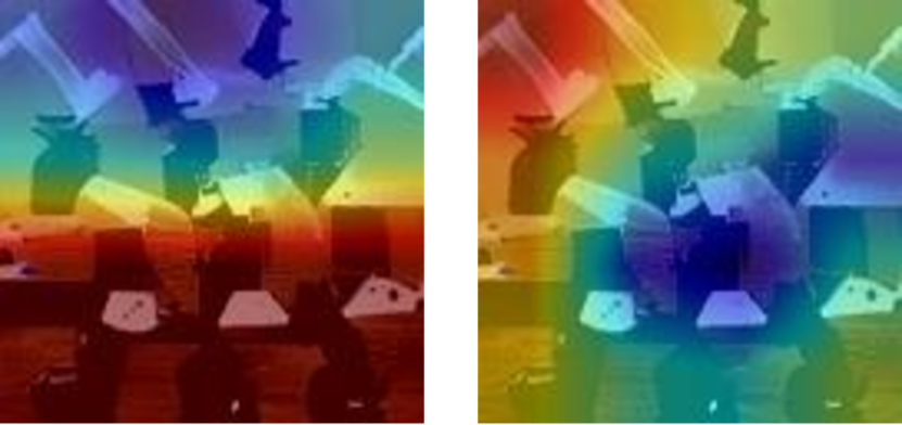
Figure 10: The visualization comparison of CAM between pre-trained model and random model using DM.

Distinguished from existing distillation methods, where the loss function is influenced by the need to fit diversity, our proposed class-relevant feature distance effectively addresses this issue by using CAM, which is calculated by utilizing a pre-trained neural network, and we utilize a ResNet-18 trained on ImageNet-1k as a proxy model for computing CAM. As shown in Figure 10, we demonstrate the difference between the visualization obtained using the pre-trained model and those obtained using a randomly initialized model. The observation indicates that there is a significant difference in the regions of interest for the two, by utilizing a pre-trained model with fixed parameters, we can better identify the feature regions that are beneficial for the classification task (i.e., larger gradients). Therefore, our proposed metric successfully leverages this strong supervisory signal to achieve data selection while eliminating the strong correlation between the loss function and the proxy model parameters.

Table 15: Ablation study of average noise initialization on GLaD.

Method ImNet-A ImNet-B ImNet-C ImNet-D ImNet-E GLaD-MTT 50.7$\pm 0.4$ 51.9$\pm 1.3$ 44.9$\pm 0.4$ 39.9$\pm 1.7$ 37.6$\pm 0.7$ + Average Initialization 51.9$\pm 1.0$ 53.5$\pm 0.7$ 46.1$\pm 0.9$ 41.0$\pm 0.7$ 39.1$\pm 1.0$ GLaD-DC 44.1$\pm 2.4$ 49.2$\pm 1.1$ 42.0$\pm 0.6$ 35.6$\pm 0.9$ 35.8$\pm 0.9$ + Average Initialization 45.4$\pm 0.6$ 48.9$\pm 0.8$ 40.6$\pm 0.7$ 36.4$\pm 0.5$ 34.8$\pm 0.3$ GLaD-DM 41.0$\pm 1.5$ 42.9$\pm 1.9$ 39.4$\pm 1.7$ 33.2$\pm 1.4$ 30.3$\pm 1.3$ + Average Initialization 41.5$\pm 1.2$ 43.2$\pm 1.6$ 39.9$\pm 1.7$ 32.2$\pm 0.9$ 30.8$\pm 1.3$

Table 16: Ablation study of average noise initialization on H-GLaD.

Method ImNet-A ImNet-B ImNet-C ImNet-D ImNet-E H-GLaD-MTT 54.1$\pm 0.5$ 56.8$\pm 0.4$ 48.9$\pm 1.3$ 45.0$\pm 0.7$ 42.1$\pm 0.6$ + Average Initialization 55.1$\pm 0.6$ 57.4$\pm 0.3$ 49.5$\pm 0.6$ 46.3$\pm 0.9$ 43.0$\pm 0.6$ H-GLaD-DC 46.5$\pm 1.0$ 50.4$\pm 0.4$ 44.5$\pm 0.6$ 37.7$\pm 1.1$ 36.9$\pm 0.7$ + Average Initialization 46.9$\pm 0.8$ 50.7$\pm 0.9$ 43.9$\pm 0.7$ 37.4$\pm 0.4$ 37.2$\pm 0.3$ H-GLaD-DM 42.6$\pm 1.6$ 44.5$\pm 0.9$ 42.3$\pm 1.4$ 34.5$\pm 1.1$ 32.3$\pm 1.3$ + Average Initialization 42.8$\pm 1.2$ 44.7$\pm 1.3$ 41.1$\pm 1.3$ 34.8$\pm 1.5$ 31.9$\pm 0.9$

B.8 Ablation Study on Average Noise Initialization

To investigate the effect of using averaged noise as initialization, we conduct ablation experiments on both GLaD and H-GLaD respectively. As shown in Table 16, averaged noise often provides a significant gain for GLaD. Indicating that using averaged noise as input tends to produce images with reduced bias that conform to the statistical characteristics of the real dataset, implying that images generated from averaged noise are usually centered within the real dataset. As aforementioned, since GLaD neglects the informative guidance from the earlier layers, leading to a lack of optimization for the main subject of the synthetic image, averaged noise can to some extent replace this operation.

As shown in Table 16, average noise initialization provides only a limited improvement for H-GLaD on MTT, while using DC and DM, averaged noise is closer to random initialization. The observation aligns with our perspective that H-GLaD requires optimization through all layers of the GAN, which has already led to optimization for the main subject information that conforms to the constraints of the loss function during the early stages of training. The role of averaged noise is then reduced to merely providing samples that better conform to statistical characteristics, which is also why we still employ averaged noise for H-GLaD to obtain a training-free optimization starting point.

Additionally, since DC tends to optimize towards classification boundary samples or noisy samples, and DM tends to substantially modify synthetic datasets to achieve feature maximum mean discrepancy optimization, neither GLaD nor H-GLaD with average noise initialization can effectively improve the performance on DC and DM. Nevertheless, MTT is most effective in preserving the primary subject information in the synthetic images, which allows for the averaging of noise and the achievement of a relatively stable improvement.

Appendix C Experimental Details

Table 17: Corresponding class names in each ImageNet-Subsets. The visualizations follow the same order.

Dataset 0 1 2 3 4 5 6 7 8 9 ImNet-A Leonberg Probiscis Monkey Rapeseed Three-Toed Sloth Cliff Dwelling Yellow Lady’s Slipper Hamster Gondola Orca Limpkin ImNet-B Spoonbill Website Lorikeet Hyena Earthstar Trollybus Echidna Pomeranian Odometer Ruddy Turnstone ImNet-C Freight Car Hummingbird Fireboat Disk Brak Bee Eater Rock Beauty Lion European Gallinule Cabbage Butterfly Goldfinch ImNet-D Ostrich Samoyed Snowbird Brabancon Griffon Chickadee Sorrel Admiral Great Gray Owl Hornbill Ringlet ImNet-E Spindle Toucan Black Swan King Penguin Potter’s Wheel Photocopier Screw Tarantula Oscilloscope Lycaenid ImNette Tench English Springer Cassette Player Chainsaw Church French Horn Garbage Truck Gas Pump Golf Ball Parachute ImWoof Australian Terrier Border Terrier Samoyed Beagle Shih-Tzu English Foxhound Rhodesian Ridgeback Dingo Golden Retriever English Sheepdog ImNet-Birds Peacock Flamingo Macaw Pelican King Penguin Bald Eagle Toucan Ostrich Black Swan Cockatoo ImNet-Fruits Pineapple Banana Strawberry Orange Lemon Pomegranate Fig Bell Pepper Cucumber Granny Smith Apple ImNet-Cats Tabby Cat Bengal Cat Persian Cat Siamese Cat Egyptian Cat Lion Tiger Jaguar Snow Leopard Lynx

C.1 Dataset

We evaluate H-GLaD on various datasets, including a low-resolution dataset CIFAR10[14] and a large number of high-resolution datasets ImageNet-Subset.

• CIFAR-10 consists of $32\times 32$ RGB images with 50,000 images for training and 10,000 images for testing. It has 10 classes in total and each class contains 5,000 images for training and 1,000 images for testing.

• ImageNet-Subset is a small dataset that is divided out from the ImageNet[40] based on certain characteristics. By aligning with the previous work, we use the same types of subsets: ImageNette (various objects)[41], ImageWoof (dogs)[41], ImageFruit (fruits) [8], ImageMeow (cats) [8], ImageSquawk (birds) [8], and ImageNet-[A, B, C, D, E] (based on ResNet50 performance) [12]. Each subset has 10 classes. The specific class name in each Imagenet-Subset is shown in Table 17.

C.2 Network Architecture

For the comparison of same-architecture performance, we employ a convolutional neural network ConvNet-3 as the backbone network as well as the test network. For low-resolution datasets, we employ a 3-depth convolutional neural network ConvNet-3 as the backbone network, consisting of three basic blocks and one fully connected layer. Each block includes a $3\times 3$ convolutional layer, instance normalization [43], ReLU non-linear activation, and a $2\times 2$ average pooling layer with a stride of 2. After the convolution blocks, a linear classifier outputs the logits. For high-resolution datasets, we employ a 5-depth convolutional neural network ConvNet-5 as the backbone network for $128\times 128$ resolution, ConvNet-5 has five duplicate blocks, which is as the same as that in ConvNet-3. For $256\times 256$ resolution, we employ ConvNet-6 as the backbone network.

For the comparison of cross-architecture performance, we also follow the previous work: ResNet-18 [1], VGG-11 [45], AlexNet [44], and ViT [2] from the DC-BENCH [46] resource.

Table 18: Detailed hyper-parameters.

(a) DM hyper-parameters

Dataset IPC Learning rate (Latent w) Learning rate (Latent f) Steps per space CIFAR-10 $1$ $10^{-2}$ $10^{1}$ $20$ $10$ $10^{-2}$ $10^{1}$ $20$ ImageNet-Subset $1$ $10^{-2}$ $10^{1}$ $20$ $10$ $10^{-2}$ $10^{1}$ $20$

(b) DC hyper-parameters

Dataset IPC inner loop outer loop Learning rate (Latent w) Learning rate (Latent f) Steps per space CIFAR-10 $1$ $1$ $1$ $10^{-3}$ $10^{0}$ $100$ $10$ $50$ $10$ $10^{-3}$ $10^{0}$ $100$ ImageNet-Subset $1$ $1$ $1$ $10^{-3}$ $10^{0}$ $100$ $10$ $50$ $10$ $10^{-3}$ $10^{0}$ $100$

(c) MTT hyper-parameters

Dataset IPC Synthetic steps Expert epochs Max expert epoch Trajectory number Learning rate (Learning rate) Learning rate (Teacher) Learning rate (Latent w) Learning rate (Latent f) Steps per space CIFAR-10 $1$ $20$ $3$ $50$ $100$ $10^{-6}$ $10^{-2}$ $10^{1}$ $10^{4}$ $100$ $10$ $20$ $3$ $50$ $100$ $10^{-6}$ $10^{-2}$ $10^{1}$ $10^{4}$ $100$ ImageNet-Subset $1$ $20$ $3$ $15$ $200$ $10^{-6}$ $10^{-2}$ $10^{1}$ $10^{4}$ $100$

C.3 Implementation details

The implementation of our proposed H-GLaD is based on the open-source code for GLaD [12], which is conducted on NVIDIA GeForce RTX 3090.

To ensure fairness, we utilize identical hyperparameters and optimization settings as GLaD. In our experiments, we also adopt the same suite of differentiable augmentations (originally from the DSA codebase [20]), including color, crop, cutout, flip, scale, and rotate. We use an SGD optimizer with momentum, $\ell_{2}$ decay. The entire distillation process continues for 1200 epochs. We evaluate the performance of the synthetic dataset by training 5 randomly initialized networks on it.

To obtain the expert trajectories used in MTT, we train a backbone model from scratch on the real dataset for 15 epochs of SGD with a learning rate of $10^{-2}$, a batch size of 256, and no momentum or regularization. To maintain the integration of different distillation methods, we do not use the ZCA whitening on both high-resolution datasets and low-resolution datasets different from previous work[8], which leads to a same-architecture performance drop, please note that our proposed H-GLaD still outperforms under the same setting. Different from GLaD which records 1000 expert trajectories for the MTT method, we only record 200 expert trajectories and thus largely reduce the computational costs. Additionally, while GLaD performs 5k optimization epochs on the synthetic dataset using MTT as the distillation method, we only perform 1k optimization epochs and achieve better performance both on same-architecture and cross-architecture settings, further proving the superiority of our H-GLaD. The detailed hyperparameters are shown in Table 18.

Appendix D More Visualizations

We provide additional visualizations of synthetic datasets generated by H-GLaD using diverse distillation methods, as shown in Figure 11, Figure 12, and Figure 13.

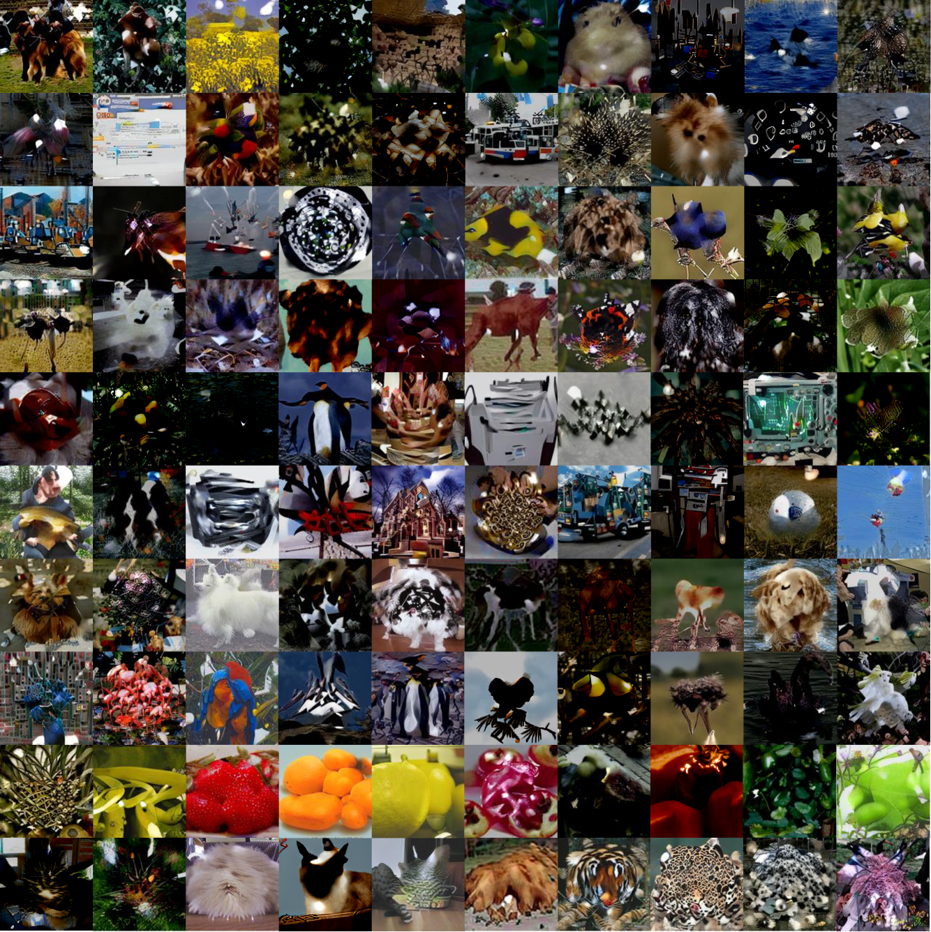
Figure 11: More visualization of the synthetic datasets using MTT.

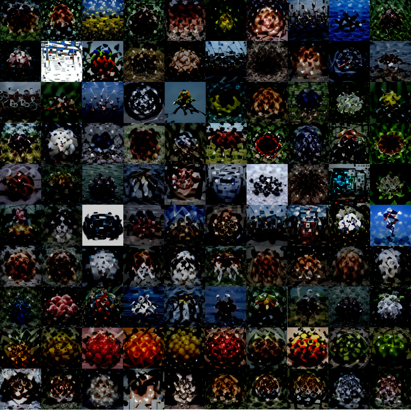
Figure 12: More visualization of the synthetic datasets using DC.

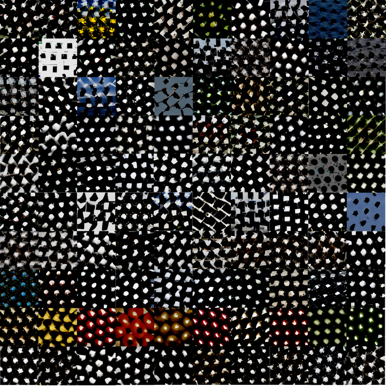
Figure 13: More visualization of the synthetic datasets using DM.

References

- [1] Kaiming He, Xiangyu Zhang, Shaoqing Ren and Jian Sun. Deep residual learning for image recognition. Proceedings of the IEEE conference on computer vision and pattern recognition, pages 770–778, 2016.
- [2] Alexey Dosovitskiy, Lucas Beyer, Alexander Kolesnikov, Dirk Weissenborn, Xiaohua Zhai, Thomas Unterthiner, Mostafa Dehghani, Matthias Minderer, Georg Heigold, Sylvain Gelly, et al. An image is worth 16x16 words: Transformers for image recognition at scale. arXiv preprint arXiv:2010.11929, 2020.
- [3] Jacob Devlin, Ming-Wei Chang, Kenton Lee and Kristina Toutanova. Bert: Pre-training of deep bidirectional transformers for language understanding. arXiv preprint arXiv:1810.04805, 2018.
- [4] Tom Brown, Benjamin Mann, Nick Ryder, Melanie Subbiah, Jared D Kaplan, Prafulla Dhariwal, Arvind Neelakantan, Pranav Shyam, Girish Sastry, Amanda Askell, et al. Language models are few-shot learners. Advances in neural information processing systems, 33:1877–1901, 2020.
- [5] Shiye Lei and Dacheng Tao. A comprehensive survey to dataset distillation arXiv preprint arXiv:2301.05603, 2023.
- [6] Tongzhou Wang, Jun-Yan Zhu, Antonio Torralba and Alexei A Efros. Dataset distillation arXiv preprint arXiv:1811.10959, 2018.
- [7] Bo Zhao, Konda Reddy Mopuri and Hakan Bilen. Dataset condensation with gradient matching. arXiv preprint arXiv:2006.05929, 2020.
- [8] George Cazenavette, Tongzhou Wang, Antonio Torralba,Alexei A Efros and Jun-Yan Zhu. Dataset distillation by matching training trajectories. Proceedings of the IEEE/CVF Conference on Computer Vision and Pattern Recognition, pages 4750–4759, 2022.
- [9] Bo Zhao and Hakan Bilen. Dataset condensation with distribution matching. Proceedings of the IEEE/CVF Winter Conference on Applications of Computer Vision, pages 6514–6523, 2023.
- [10] Bo Zhao and Hakan Bilen. Synthesizing informative training samples with gan. arXiv preprint arXiv:2204.07513, 2022.
- [11] Songhua Liu, Kai Wang, Xingyi Yang, Jingwen Ye and Xinchao Wang. Dataset distillation via factorization. Advances in Neural Information Processing Systems, 35:1100–1113, 2022.
- [12] George Cazenavette, Tongzhou Wang, Antonio Torralba, Alexei A Efros and Jun-Yan Zhu. Generalizing Dataset Distillation via Deep Generative Prior. Proceedings of the IEEE/CVF Conference on Computer Vision and Pattern Recognition, pages 3739–3748, 2023.
- [13] DongHyeok Shin, Seungjae Shin and Il-chul Moon. Frequency Domain-Based Dataset Distillation. Thirty-seventh Conference on Neural Information Processing Systems, 2023.
- [14] Alex Krizhevsky, Geoffrey Hinton, et al. Learning multiple layers of features from tiny images. Toronto, ON, Canada, 2009.
- [15] Weihao Xia, Yulun Zhang, Yujiu Yang, Jing-Hao Xue, Bolei Zhou and Ming-Hsuan Yang. Gan inversion: A survey. IEEE Transactions on Pattern Analysis and Machine Intelligence, 45(3):3121–3138, 2022.
- [16] Ondrej Bohdal, Yongxin Yang and Timothy Hospedales. Flexible dataset distillation: Learn labels instead of images. arXiv preprint arXiv:2006.08572, 2020.
- [17] Timothy Nguyen, Zhourong Chen and Jaehoon Lee. Dataset meta-learning from kernel ridge-regression. arXiv preprint arXiv:2011.00050, 2020.
- [18] Timothy Nguyen, Roman Novak, Lechao Xiao and Jaehoon Lee. Dataset distillation with infinitely wide convolutional networks. Advances in Neural Information Processing Systems, 34:5186–5198, 2021.
- [19] Yongchao Zhou, Ehsan Nezhadarya and Jimmy Ba. Dataset distillation using neural feature regression. Advances in Neural Information Processing Systems, 35:9813–9827, 2022.
- [20] Bo Zhao and Hakan Bilen. Dataset condensation with differentiable siamese augmentation. International Conference on Machine Learning, pages 12674–12685. PMLR, 2021.
- [21] Saehyung Lee, Sanghyuk Chun, Sangwon Jung, Sangdoo Yun and Sungroh Yoon. Dataset condensation with contrastive signals. International Conference on Machine Learning, pages 12352–12364. PMLR, 2022.
- [22] Kai Wang, Bo Zhao, Xiangyu Peng, Zheng Zhu, Shuo Yang, Shuo Wang, Guan Huang, Hakan Bilen, Xinchao Wang and Yang You. Cafe: Learning to condense dataset by aligning features. Proceedings of the IEEE/CVF Conference on Computer Vision and Pattern Recognition, pages 12196–12205, 2022.
- [23] Justin Cui, Ruochen Wang, Si Si and Cho-Jui Hsieh. Scaling up dataset distillation to imagenet-1k with constant memory. International Conference on Machine Learning, pages 6565–6590. PMLR, 2023.
- [24] Ahmad Sajedi, Samir Khaki, Ehsan Amjadian, Lucy Z Liu, Yuri A Lawryshyn and Konstantinos N PlataniLawryshyn otis. Datadam: Efficient dataset distillation with attention matching. Proceedings of the IEEE/CVF International Conference on Computer Vision., pages 17097–17107, 2023.
- [25] Ganlong Zhao, Guanbin Li, Yipeng Qin and Yizhou YU. Improved distribution matching for dataset condensation. Proceedings of the IEEE/CVF Conference on Computer Vision and Pattern Recognition., pages 7856–7865, 2023.
- [26] Jang-Hyun Kim, Jinuk Kim, Seong Joon Oh, Sangdoo Yun, Hwanjun Song, Joonhyun Jeong, Jung-Woo Ha and Hyun Oh Song. Dataset condensation via efficient synthetic-data parameterization. International Conference on Machine Learning, pages 11102–11118. PMLR, 2022.
- [27] Antonia Creswell, Tom White, Vincent Dumoulin, Kai Arulkumaran, Biswa Sengupta and Anil A Bharath. Generative adversarial networks: An overview. IEEE signal processing magazine, 35(1), 53–65, 2018.
- [28] Lucy Chai, Jonas Wulff and Phillip Isola. Using latent space regression to analyze and leverage compositionality in GANs. arXiv preprint arXiv:2103.10426, 2021.
- [29] Lucy Chai, Jun-Yan Zhu, Eli Shechtman, Phillip Isola and Richard Zhang. Ensembling with deep generative views. Proceedings of the IEEE/CVF Conference on Computer Vision and Pattern Recognition, pages 14997–15007, 2021.
- [30] Minyoung Huh, Richard Zhang, Jun-Yan Zhu, Sylvain Paris and Aaron Hertzmann. Transforming and projecting images into class-conditional generative networks. Computer Vision–ECCV 2020: 16th European Conference, Glasgow, UK, August 23–28, 2020, Proceedings, Part II 16, pages 17–34, 2020.
- [31] Ayush Tewari, Mohamed Elgharib, Florian Bernard, Hans-Peter Seidel, Patrick Pérez, Michael Zollhöfer and Christian Theobalt. Pie: Portrait image embedding for semantic control. ACM Transactions on Graphics (TOG), 39(6):1–14, 2020.
- [32] Andrew Brock, Theodore Lim, James M Ritchie and Nick Weston. Neural photo editing with introspective adversarial networks. arXiv preprint arXiv:1609.07093, 2016.
- [33] Andrew Brock, Jeff Donahue and Karen Simonyan. Large scale GAN training for high fidelity natural image synthesis. arXiv preprint arXiv:1809.11096, 2018.
- [34] Axel Sauer, Katja Schwarz and Andreas Geiger. Stylegan-xl: Scaling stylegan to large diverse datasets. ACM SIGGRAPH 2022 conference proceedings, pages 1–10, 2022.
- [35] Giannis Daras, Joseph Dean, Ajil Jalal and Alexandros G Dimakis. Intermediate layer optimization for inverse problems using deep generative models. arXiv preprint arXiv:2102.07364, 2021.
- [36] Hao Fang, Bin Chen, Xuan Wang, Zhi Wang and Shu-Tao Xia. GIFD: A Generative Gradient Inversion Method with Feature Domain Optimization. Proceedings of the IEEE/CVF International Conference on Computer Vision, pages 4967–4976, 2023.
- [37] Hao Fang, Yixiang Qiu, Hongyao Yu, Wenbo Yu, Jiawei Kong, Baoli Chong, Bin Chen and Xuan Wang and Shu-Tao Xia. Privacy Leakage on DNNs: A Survey of Model Inversion Attacks and Defenses. arXiv preprint arXiv:2402.04013
- [38] Yanqing Liu, Jianyang Gu, Kai Wang, Zheng Zhu, Wei Jiang and Yang You. DREAM: Efficient Dataset Distillation by Representative Matching. arXiv preprint arXiv:2302.14416, 2023.
- [39] R. R. Selvaraju, M. Cogswell, A. Das, R. Vedantam, D. Parikh, and D. Batra. Grad-cam: Visual explanations from deep networks via gradient-based localization. Proceedings of the IEEE/CVF International Conference on Computer Vision, pages 618–626, 2017.
- [40] Jia Deng, Wei Dong, Richard Socher, Li-Jia Li, Kai Li and Li Fei-Fei. Imagenet: A large-scale hierarchical image database. IEEE conference on computer vision and pattern recognition, pages 248–255, 2009
- [41] Jeremy Howard. A smaller subset of 10 easily classified classes from Imagenet, and a little more french. URL https://github. com/fastai/imagenette, 2019.
- [42] Spyros Gidaris and Niko Komodakis. Dynamic few-shot visual learning without forgetting Proceedings of the IEEE conference on computer vision and pattern recognition, pages 4367–4375, 2018.
- [43] Dmitry Ulyanov, Andrea Vedaldi and Victor Lempitsky. Instance normalization: The missing ingredient for fast stylization. arXiv preprint arXiv:1607.08022, 2016.
- [44] Alex Krizhevsky, Ilya Sutskever and Geoffrey E Hinton. Imagenet classification with deep convolutional neural networks. Advances in neural information processing systems, 25, 2012.
- [45] Karen Simonyan and Andrew Zisserman. Very deep convolutional networks for large-scale image recognition. arXiv preprint arXiv:1409.1556, 2014.
- [46] Justin Cui, Ruochen Wang, Si Si and Cho-Jui Hsieh. DC-BENCH: Dataset condensation benchmark. Advances in Neural Information Processing Systems, 35:810–822, 2022.