General Distribution Learning: A theoretical framework for Deep Learning

Abstract

There remain numerous unanswered research questions on deep learning (DL) within the classical learning theory framework. These include the remarkable generalization capabilities of overparameterized neural networks (NNs), the efficient optimization performance despite non-convexity of objectives, the mechanism of flat minima for generalization, and the exceptional performance of deep architectures in solving physical problems. This paper introduces General Distribution Learning (GD Learning), a novel theoretical learning framework designed to address a comprehensive range of machine learning and statistical tasks, including classification, regression and parameter estimation. Departing from traditional statistical machine learning, GD Learning focuses on the true underlying distribution. In GD Learning, learning error, corresponding to the expected error in the classical statistical learning framework, is divided into fitting errors due to models and algorithms, as well as sampling errors introduced by limited sampling data. The framework significantly incorporates prior knowledge, especially in scenarios characterized by data scarcity, thereby enhancing performance. Within the GD Learning framework, we demonstrate that the global optimal solutions in non-convex optimization can be approached by minimizing the gradient norm and the non-uniformity of the eigenvalues of the model’s Jacobian matrix. This insight leads to the development of the gradient structure control algorithm. GD Learning also offers fresh insights into the questions on deep learning, including overparameterization and non-convex optimization, bias-variance trade-off, and the mechanism of flat minima. The article structure is as follows: An initial overview of GD Learning is presented, outlining its fundamental components and a schematic diagram. We then delve into the components of the proposed framework, analyzing the standard loss function, fitting model, gradient structure control algorithm, and establishing an upper bound on learning error. Finally, we illustrate how GD Learning unifies classification and regression problems and addresses the unanswered questions on DL within the classical learning theory framework.

Keywords: distribution learning, deep learning, non-convex optimization

1 Introduction

Along with the remarkable practical achievements of deep learning, several fundamental questions on DL remain unanswered within the classical learning theory framework. These include:

• why can deep neural networks (DNNs) avoid overfitting despite their immense capacity, and how do they surpass shallow architectures?

• how do DNNs overcome the curse of dimensionality, and why do optimization algorithms often succeed in finding satisfactory solutions despite non-convex non-linear, and often non-smooth DL objectives?

• which aspects of an architecture affect the performance of the associated models and the mechanisms behind these influences?

Delving into the reasons and factors that govern the performance of DNNs not only enhances the interpretability for DNNs but also facilitates the development of more principled and reliable architecture designs.

Extensive empirical evidence indicates that, in addition to expressivity (Leshno et al., 1993; Barron, 1993) and trainability (Choromańska et al., 2014; Kawaguchi, 2016), the generalization of DNNs significantly influences prediction performance (Kawaguchi et al., 2017). Generalization error, a measure of a model’s predictive ability on unseen data, is a critical aspect of learning models. Some classical theory work attributes generalization ability to the utilization of a low-complexity class of hypotheses and proposes various complexity measures to control generalization error. These include the Vapnik-Chervonenkis (VC) dimension (Wu, 2021), Rademacher complexity (Bartlett and Mendelson, 2003), and uniform stability (Mukherjee et al., 2006; Bousquet and Elisseeff, 2002). However, recent studies by (Zhang et al., 2016, 2021; He et al., 2015a; Belkin et al., 2018a) demonstrate that high-capacity DNNs can still generalize well with genuine labels, yet generalize poorly when trained with random labels. This apparent contradiction with the traditional understanding of overfitting in complex models highlights the need for further investigation (Vapnik and Alexey, 1971; Wu, 2021; Bartlett and Mendelson, 2003).

Distribution learning (estimation), a cornerstone in various fields such as machine learning, theoretical and applied statistics, information theory and communication applications, has a rich history. The distribution, described by a probability density/mass function (PDF/PMF), completely characterizes the ”behavior” of a random variable, making distribution learning fundamental for investigating the properties of a given dataset and for efficient data mining. The goal of distribution learning is to estimate the true underlying distribution from a given sample set. The majority of machine learning tasks can be framed within the distribution learning context, with both classification and regression problems mathematically represented by learning the conditional probability distributions between features and labels. In particular, generative learning corresponds to learning the underlying joint distribution. Consequently, approaching machine learning and deep learning from the perspective of distribution learning is a logical and coherent choice, given its inherent suitability for these tasks.

In this paper, we introduce a novel framework, General Distribution Learning (GD Learning). Departing from the traditional statistical learning framework, GD Learning focuses on the true underlying distribution and utilizes norms to measure learning error. In this framework, learning error is categorized into fitting errors caused by models and algorithms, as well as sampling errors resulting from limited sampling data. The GD Learning framework consists of a standard loss function, a fitting model, prior knowledge, and a gradient structure control algorithm. The standard loss function, a constrained function, encompasses common loss functions and can be expressed as a Young–Fenchel loss function or a Bregman divergence. The fitting model in GD Learning is used to estimate the parameters of a distribution. It is important to note that when the distribution to be learned has finite supports, the support probabilities are the parameters to be estimated. The gradient structure control algorithm is designed to minimize the gradient norm and the structural error which is bounded by the non-uniformity of the model’s Jacobian eigenvalues. A key departure from traditional optimization algorithms is that the gradient structure control algorithm optimizes for stationary points rather than global optima. Within the GD Learning framework, we demonstrate that the global optimal solution to non-convex optimization problems, such as fitting error minimization, can be approached by the gradient structure control algorithm. GD Learning also offers a fresh perspective on deep learning issues, including overparameterization, non-convex optimization, the bias-variance trade-off, and the mechanisms behind flat minima.

The article is organized as follows: In Section 2, we delve into related work, reviewing learning theory, modern deep learning analysis, and distribution learning methods. In Section 3 we define the fundamental concepts and objects utilized in this paper. In Section 4 we provide an overview of GD Learning, detailing its basic components and schematic diagram. In Section 5, we define the standard loss and demonstrate its equivalence to both the Young-Fenchel loss and Bregman divergence. In Section 6, we introduce the concept of a standard structural model and examine the factors that influence it. In Section 7, we propose the gradient structure control algorithm and establish that the global optimal solution for non-convex optimization problems, such as fitting error minimization, can be achieved by minimizing the gradient norm and the structural error, which is bounded by the non-uniformity of the eigenvalues of the model’s Jacobian matrix. In Section 8, we derive the theoretical bounds for learning error, providing insights into the performance of GD Learning. In Section 9, we illustrate how GD Learning unifies classification and regression problems, and address the questions that remain unanswered within the classical learning theory framework. In Section 10, we summarize our findings and discuss their broader implications for the field.

2 Related work

In this section, we provide an overview of learning theory, modern approaches for analyzing deep learning, and distribution learning methods.

2.1 Learning theory

We begin by presenting a succinct summary of the classical mathematical and statistical theory underlying machine learning tasks and algorithms which, in their most general form, can be formulated as follows.

Definition 1 (Learning task)

In a learning task, one is given a loss function $\ell:\mathcal{M}(\mathcal{X},\mathcal{Y})\times\mathcal{Z}\to\mathbb{R}$ and training data $s^{n}=\{z^{(i)}\}_{i=1}^{n}$ which is generated by independent and identically distributed (i.i.d.) sampling according to the unknown true distribution $Z\sim\bar{q}$, where $Z$ are random variables that take the values in $\mathcal{Z}$. The objective is to construct a learning algorithm $\mathcal{A}$ that uses training data $s$ to find a model $f_{s}$ that performs well on the whole data, where $f_{s}=\mathcal{A}(s)\in\mathcal{F}$, the hypothesis set $\mathcal{F}\subset\mathcal{M}(\mathcal{X},\mathcal{Y})$, and the mapping $\mathcal{A}:s^{n}\to\mathcal{F}$. Here, performance is measured via $\mathbb{E}_{Z}\ell(f_{s},z)$.

The above definition can describe a supervised learning task. It is noteworthy that unsupervised and semi-supervised learning tasks are also treated as supervised learning tasks when the training data comprises solely features $x$. Specifically, one can construct a label $y=T(x)$ where $x\in\mathcal{X}$, $T(x)\in\mathcal{Y}$, with $T:\mathcal{X}\to\mathcal{Y}$ representing a transformation. Consequently, the learning task is to find a model $f_{s}$ that approximates the transformation $T$, which is often pursued to learn feature representations or invariances.

Given a hypothesis set, a widely utilized learning algorithm is empirical risk minimization (ERM), which minimizes the average loss on the given training data, as described in the subsequent definitions.

Definition 2 (Empirical risk)

For a given training dataset $s$ and a function $f\in\mathcal{M}(\mathcal{X},\mathcal{Y})$, the empirical risk is defined as:

$$\widehat{\mathcal{R}}_{s}(f):=\frac{1}{n}\sum_{i=1}^{n}\ell(f,z^{(i)}).$$ (1)

Definition 3 (Expected risk)

For a function $f\in\mathcal{M}(\mathcal{X},\mathcal{Y})$, the expected risk is defined by:

$$\mathcal{R}(f):=\mathbb{E}_{Z\sim\bar{q}}[\ell(f,z^{(i)})].$$ (2)

Let $f_{s}=\mathcal{A}(s)$, then the expected risk of the model $f_{s}$ is given by

$$\mathcal{R}(f_{s})=\mathbb{E}_{Z\sim\bar{q}}[\ell(f_{s},z^{(i)})].$$ (3)

Definition 4 (ERM learning algorithm)

Given a hypothesis set $\mathcal{F}$, an Empirical Risk Minimization (ERM) algorithm $\mathcal{A}^{erm}$ chooses a function $\widehat{f}_{s}\in\mathcal{F}$ that minimizes the empirical risk for the training data $s$, i.e.,

$$\mathcal{A}^{erm}(s)\in\arg\min_{f\in\mathcal{F}}\widehat{\mathcal{R}}_{s}(f).$$ (4)

Definition 5 (Bayes-optimal function)

A function $f^{\star}\in\mathcal{M}(\mathcal{X},\mathcal{Y})$ achieving the minimum risk, its Bayes risk is

$$\mathcal{R}^{\star}:=\inf_{f\in\mathcal{M}(\mathcal{X},\mathcal{Y})}\mathcal{R}(f),$$ (5)

Definition 6 (Errors of learning)

Let $f^{\star}_{\mathcal{F}}\in\arg\min_{f\in\mathcal{F}}(f)$ represent the best approximation in $\mathcal{F}$, the optimization error denoted by $e_{\rm opt}$, generalization error denoted by $e_{\rm gen}$ and approximation error denoted by $e_{\rm approx}$ are defined as follows

$$e_{\rm opt}(\mathcal{A},\mathcal{F}):=\widehat{\mathcal{R}}_{s}(f_{s})-\widehat{\mathcal{R}}_{s}(\widehat{f}_{s})\geq\widehat{\mathcal{R}}_{s}(f_{s})-\widehat{\mathcal{R}}_{s}(f^{\star}_{\mathcal{F}})$$ (6)

$$e_{\rm gen}(\mathcal{F}):=\sup_{f\in\mathcal{F}}|\mathcal{R}(f)-\widehat{\mathcal{R}}_{s}(f)|\geq\max\{|\mathcal{R}(f_{s})-\widehat{\mathcal{R}}_{s}(f_{s})|,|\mathcal{R}(f_{\mathcal{F}}^{\star})-\widehat{\mathcal{R}}_{s}(f^{\star}_{\mathcal{F}})|\}$$

$$e_{\rm approx}(\mathcal{F}):=\mathcal{R}(f^{\star}_{\mathcal{F}})-\mathcal{R}^{\star}.$$

The error $\mathcal{R}(f_{s})-\mathcal{R}^{\star}$ can then be bounded by:

$$\mathcal{R}(f_{s})-\mathcal{R}^{\star} =\mathcal{R}(f_{s})-\widehat{\mathcal{R}}_{s}(f_{s})+\widehat{\mathcal{R}}_{s}(f_{s})-\widehat{\mathcal{R}}_{s}(f^{\star}_{\mathcal{F}})$$ (7)

$$+\widehat{\mathcal{R}}_{s}(f^{\star}_{\mathcal{F}})-\mathcal{R}_{s}(f^{\star}_{\mathcal{F}})+\mathcal{R}_{s}(f^{\star}_{\mathcal{F}})-\mathcal{R}^{\star}$$

$$\leq e_{\rm opt}(\mathcal{A},\mathcal{F})+2e_{\rm gen}(\mathcal{F})+e_{\rm approx}(\mathcal{F}).$$

The optimization error $e_{\rm opt}$ is primarily influenced by the algorithm $\mathcal{A}$ that is used to find the model $f_{s}$ in the hypothesis set $\mathcal{F}$ for given training data $s$. By far, the gradient-based methods are the most prevalent approach to address this issue, leveraging their ability to accurately and efficiently compute the derivatives by automatic differentiation in a lot of widely used models. Owing to the hierarchical structure of neural networks, the back-propagation algorithm has been proposed to efficiently calculate the gradient with respect to the loss function (Kelley, 1960; Dreyfus, 1962; Rumelhart et al., 1986; Griewank and Walther, 2000). Stochastic gradient descent (SGD), introduced by Robbins (1951) is a typical gradient-based method used to identify the unique minimum of a convex function (Kiefer and Wolfowitz, 1952). In scenarios where the objective function is non-convex, SGD generally converges to a stationary point, which may be either a local minimum, a local maximum, or a saddle point. Nonetheless, there are indeed conditions under which convergence to local minima is guaranteed (Nemirovski et al., 2008; Ge et al., 2015; Lee et al., 2016; Jentzen et al., 2018).

The universal approximation theorem (Lewicki and Marino, 2003; ichi Funahashi, 1989; Hornik et al., 1989; Leshno et al., 1993) states that neural networks with only 2 layers can approximate any continuous function defined on a compact set up to arbitrary precision. This implies that the approximation error, $e_{\rm approx}$, decreases as the model’s complexity increases. The generalization error, $e_{\rm gen}(\mathcal{F})$, is defined as the difference between the true risk and the empirical risk. To bound the generalization error, Hoeffding’s inequality (Hoeffding, 1994) alongside the union bound directly provides the PAC (Probably Approximately Correct) bound (Valiant, 1984). The PAC bound is described as follows:

$$\Pr[e_{\rm gen}(\mathcal{F})\leq\varepsilon(\frac{1}{\delta},\frac{1}{n})]\geq 1-\delta$$ (8)

In simpler terms, when the sample $s^{n}$ is chosen randomly, good generalization is ensured with a high probability, at least $1-\delta$, by minimizing $\varepsilon(\frac{1}{\delta},\frac{1}{n})$. The function $\varepsilon$ depends mainly on the number of samples $n$ and the confidence parameter $\delta$. The uniform convergence bound is a classical type of generalization bounds based on measures of complexity of the set $\mathcal{F}$, such as the VC-dimension (Wu, 2021) and the Rademacher complexity (Bartlett and Mendelson, 2003)). These bounds are applicable to all the hypotheses within $\mathcal{F}$ and are expressed mathematically as follows:

$$\Pr[e_{\rm gen}(\mathcal{F})\leq\varepsilon(\frac{1}{\delta},\frac{1}{n},\mathcal{F})]\geq 1-\delta$$ (9)

These bounds, characterized by the supremum operator $\sup_{f\in\mathcal{F}}$, can be seen as a worst-case analysis.

A potential drawback of the uniform convergence bounds is that they are independent of the learning algorithm, i.e., they do not take into account the way the hypothesis space is explored. To tackle this issue, algorithm-dependent bounds have been proposed to take advantage of some particularities of the learning algorithm, such as its uniform stability (Bousquet and Elisseeff, 2002) or robustness (Xu and Mannor, 2010). In such instances, the bounds obtained hold for the hypothesis set $\mathcal{A}(s)\in\mathcal{F}$ which is learned with the algorithm $\mathcal{A}$ using the sample $s$. The form of such bounds is represented as:

$$\Pr[e_{\rm gen}(\mathcal{A},\mathcal{F})\leq\varepsilon(\frac{1}{\delta},\frac{1}{n},\mathcal{A})]\geq 1-\delta$$ (10)

For instance, the work presented by Hardt et al. (2015) utilizes this approach to derive generalization bounds for hypotheses learned by stochastic gradient descent.

The classical trade-off highlights the need to balance model complexity and generalization. While simpler models may suffer from high bias, overly complex ones can overfit noise (high variance). However, reconciling the classical bias-variance trade-off with the empirical observation of good generalization, despite achieving zero empirical risk on noisy data using DNNs with a regression loss, presents a significant challenge (Belkin et al., 2018b). Generally speaking, in deep learning, overparameterization and perfectly fitting noisy data do not exclude good generalization performance. Moreover, empirical evidence across various modeling techniques, including DNNs, decision trees, random features, linear models, indicates that test error can decrease even below the sweet-spot in the U-shaped bias-variance curve when further increasing the number of parameters (Belkin et al., 2018a; Geiger et al., 2019; Nakkiran et al., 2019). This phenomenon is often referred to as the double descent curve or benign overfitting, as illustrated in Figure 1.

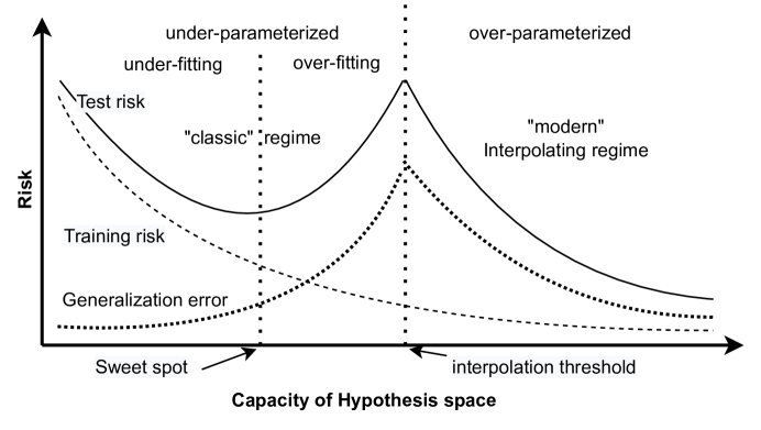
Figure 1: The double descent risk curve, which incorporates the U-shaped risk curve (i.e., the ”classical” regime) together with the observed behavior from using high capacity function classes (i.e., the ”modern” interpolating regime), separated by the interpolation threshold. The predictors to the right of the interpolation threshold have zero training risk (Belkin et al., 2018a).

The available body of evidence suggests that classical tools from statistical learning theory alone, such as uniform convergence, algorithmic stability, or bias-variance trade-off may be unable to fully capture the behavior of DNNs (Zhang et al., 2016; Nagarajan and Kolter, 2019).

2.2 Deep learning theory

Deep learning poses several mysteries within the conventional learning theory framework, including the outstanding generalization ability of overparameterized neural networks, the impact of depth in deep architectures, the apparent absence of the curse of dimensionality, the surprisingly successful optimization performance despite the non-convexity of the problem, understanding what features are learned, why deep architectures perform exceptionally well in solving physical problems, and which fine aspects of an architecture affect the behavior of a learning task in which way. Theoretical insights into these problems from prior research have predominantly followed two main avenues: architecture of model and optimization algorithm.

Regarding model architecture, Hanin and Sellke (2017); Kidger and Lyons (2019) show that very narrow neural networks can remain universally approximative with an appropriate selection of depth. More specifically, an increase in the depth of a neural network architecture has the effect of increasing its expressiveness exponentially (Poole et al., 2016; Zhang et al., 2023). Increasing the depth of a neural network architecture naturally yields a highly overparameterized model, whose loss landscape is known for a proliferation of local minima and saddle points (Dauphin et al., 2014). Overparameterization is widely believed to be crucial for the generalization ability of DNNs, as supported by studies like (Du et al., 2018; Yun et al., 2018; Chizat et al., 2018; Arjevani and Field, 2022).

It is also widely believed that the generalization of highly overparameterized models cannot be adequately explained without accounting for stochastic optimization algorithms whose inherent stochasticity performs implicit regularization, guiding parameters towards flat plateaus with lower generalization errors (Keskar et al., 2016; Chaudhari and Soatto, 2017). First-order optimization methods, such as SGD, have been demonstrated to be more efficient in escaping from saddle points and converge to flat minima (Dauphin et al., 2014; Lee et al., 2019). To identify the flat minima, numerous mathematical definitions of flatness exist, with a prevalent one being the largest eigenvalue of the Hessian matrix of the loss function with respect to the model parameters on the training set, denoted as $\lambda_{\max}$ (Jastrzebski et al., 2017; Lewkowycz et al., 2020; Dinh et al., 2017). The work of Jacot et al. (2018) elucidates that the evolution of the trainable parameters in continuous-width DNNs during training can be captured by the neural tangent kernel (NTK). Recent studies demonstrate that with specialized scaling and random initialization, the dynamics of gradient descent (GD) in continuous-width multi-layer neural networks can be tracked via NTK and the convergence to the global optimum with a linear rate can be proved (Du et al., 2018; Zou et al., 2018; Allen-Zhu et al., 2018) . An alternative research direction attempts to examine the infinite-width neural network from a mean-field perspective (Sirignano and Spiliopoulos, 2018; Mei et al., 2018; Chizat and Bach, 2018). The key idea is to characterize the learning dynamics of noisy SGD as the gradient flows over the space of the probability distribution of the neural network parameters. NTK and mean-field methods provide a fundamental understanding on training dynamics and convergence property.

Nonetheless, from the perspective of objective function optimization, training DNNs is a non-convex optimization problem. Yet empirical observations indicate that even simple algorithms, such as SGD, tend to converge to the global minimum. The mechanism behind this cannot be explained by classical convex optimization theory. A popular claim in the literature is that overparameterization also plays an important role in non-convex optimization (Du et al., 2018; Zou et al., 2018; Allen-Zhu et al., 2018; Sirignano and Spiliopoulos, 2018; Mei et al., 2018; Chizat and Bach, 2018).

Accumulating evidence indicates that the exceptional performance of DNNs is attributed to a confluence of factors, including their architectural design, optimization algorithms, and even training data.

2.3 Distribution learning

In statistical data analysis, determining the probability density function (PDF) or probability mass function (PMF) from a limited number of random samples is a common task, especially when dealing with complex systems where accurate modeling is challenging. Generally, there are three main approaches to this problem: parametric, semi-parametric, and non-parametric models.

Parametric models assume that the data follows a specific distribution with unknown parameters. Examples include the Gaussian model, Gaussian Mixture models (GMMs), and distributions from the generalized exponential family. A major limitation of these methods is that they apply quite simple parametric assumptions, which may not be sufficient or verifiable in practice. For instance, GMMs are based on the first few moments, and thus provide a poor fit for some distributions, including heavy-tailed processes (Rahman et al., 2008).

Non-parametric models estimate the PDF/PMF based on data points without making assumptions about the underlying distribution (Härdle et al., 2004). Examples include the histogram (Sturges, 1926; Scott, 1979; Freedman and Diaconis, 1981) and kernel density estimation (KDE) (Parzen, 1962; Silverman, 2018; Hall et al., 2004). While these methods are more flexible, they may suffer from overfitting or poor performance in high-dimensional spaces due to the curse of dimensionality.

Semi-parametric models (McLachlan et al., 2019) strike a balance between parametric and non-parametric approaches. They do not assume the a prior-shape of the PDF/PMF to estimate as non-parametric techniques. However, unlike the non-parametric methods, the complexity of the model is fixed in advance, in order to avoid a prohibitive increase of the number of parameters with the size of the dataset, and to limit the risk of overfitting. Finite mixture models are commonly used to serve this purpose.

Statistical methods for determining the parameters of a model conditional on the data, including the standard likelihood method (Aldrich, 1997; Hald, 1999; Meeker et al., 2022), M-estimators (Huber, 1964, 1973), and Bayesian methods (MacKay, 2003; Sivia and Skilling, 2006; Murphy, 2022), have been widely employed. The Maximum Likelihood (MLE), introduced by Fisher (Aldrich, 1997), is commonly used in data regression, with earlier ideas discussed by Daniel Bernoulli and and Gauss (Hald, 1999). In 1964, Huber (1964) proposed a generalization of the maximum likelihood objective function. In 1973 Huber (1973) extended the idea of using M-estimators for solution of regression problems. However, traditional estimators struggle in high-dimensional space: because the required sample size or computational complexity often explodes geometrically with increasing dimensionality, they have almost no practical value for high-dimensional data.

Recently, neural network-based approaches have been proposed for PDF/PMF estimation and have shown promising results in problems with high-dimensional data points such as images. There are mainly two families of such neural density estimators: auto-regressive models (Larochelle and Murray, 2011; Papamakarios et al., 2017) and normalizing flows (Rezende and Mohamed, 2015; Dinh et al., 2016). Autoregression-based neural density estimators decompose the density into the product of conditional densities based on probability chain rule $p(x)=\prod_{i}p(x_{i}|x_{1:i-1})$. Each conditional probability $p(x_{i}|x_{1:i-1})$ is modeled by a parametric density (e.g., Gaussian or mixture of Gaussian), and the parameters are learned by neural networks. Density estimators based on normalizing flows represent $x$ as an invertible transformation of a latent variable $z$ with known density, where the invertible transformation is a composition of a series of simple functions whose Jacobian is easy to compute. The parameters of these component functions are then learned by neural networks. As suggested by Kingma et al. (2016), both of these are special cases of the following general framework. Given a differentiable and invertible mapping $G:\mathbb{R}^{n}\to\mathbb{R}^{n}$ and a base density $p_{Z}(z)$, the density of $X=G(Z)$ can be represented using the change of variable rule as follows:

$$p_{X}(x)=p_{Z}(z)|\mathrm{det}(\mathbf{J}_{z})|^{-1}$$ (11)

where $\mathbf{J}_{z}=(\partial G(z))/\partial z^{\top}$ is the Jacobian matrix of function $G(\cdot)$ at point $\mathbf{z}$. Density estimation at $\mathbf{x}$ can be solved if the base density $p_{Z}(z)$ is known and the determinant of the Jacobian matrix is feasible to calculate. To achieve this, previous neural density estimators have to impose heavy constraints on the model architecture. For example Papamakarios et al. (2017); Dinh et al. (2016); Kingma et al. (2016) require the Jacobian to be triangular.

3 Preliminaries

3.1 Notation

• The set of real numbers is denoted by $\mathbb{R}$, and the cardinality of set $\mathcal{Z}$ is denoted by $|\mathcal{Z}|$.

• The $|\mathcal{Z}|$-dimensional probability simplex is denoted by $\Delta^{|\mathcal{Z}|}:=\{p\in\mathbb{R}_{+}^{|\mathcal{Z}|}\colon\|p\|_{1}=1\}$.

• Random variables are denoted using upper case letters such as $X,Y$ which take the values in set $\mathcal{X}$, and $\mathcal{Y}$, respectively.

• The expectation of a random variable $X$ is denoted by $\mathbb{E}{[X]}$ or $\mathbb{E}_{X}[X]$, with $\mathbb{E}_{X\sim p}[X]$ when the distribution of $X$ is specified.

• The space of fitting models, which is a set of functions endowed with some structure, is represented by $\mathcal{F}({\Theta})=\{f(\theta):\theta\in\Theta\}$, where $\Theta$ denotes the parameter space.

• The Fréchet sub-differential is defined as $\partial f(x)=\{s\in\mathbb{R}^{n}|\lim_{y\to x}\frac{f(y)-f(x)-\langle s,y-s\rangle}{\|y-x\|}\geq 0\}$ (see e.g., (Li et al., 2020),Page 27). If $f(x)$ is smooth and convex, the Fréchet sub-differential $\hat{\partial}f(x)$ reduces to the usual gradient, i.e., $\partial f(x)=\{\nabla f(x)\}$.

• The Fenchel conjugate of a function $\Omega$ is denoted by $\Omega^{*}(f):=\sup_{p\in\mathrm{dom}(\Omega)}\langle p,f\rangle-\Omega(p)$. By default, $\Omega$ is a continuous strictly convex function, and its gradient with respect to $p$ is denoted by $p_{\Omega}^{*}$.

• The Bregman divergence associated with a convex function $\Omega$ and its subgradient $f$ is defined as $B_{\Omega}(q,p)=\Omega(q)-\Omega(p)-f^{\top}(q-p)$, where $f\in\partial\Omega(p)$.

• The Kullback-Leibler (KL) divergence is denoted by

  $$D_{KL}(p\|f):=\sum_{i}p_{i}\log\frac{p_{i}}{f_{i}}-\sum_{i}p_{i}+\sum_{i}f_{i}.$$ (12)

• The largest and smallest eigenvalues of matrix $A$ are denoted by $\lambda_{\max}(A)$ and $\lambda_{\min}(A)$, respectively.

3.2 Setting and basics

The random pair $Z=(X,Y)$ follows the distribution $\bar{q}$ and takes the values in the product space $\mathcal{Z}=\mathcal{X}\times\mathcal{Y}$, where $\mathcal{X}$ represents the input feature space and $\mathcal{Y}$ represents the label set. The training data, denoted by an $n$-tuple $s^{n}=\{z{(i)}\}_{i=1}^{n}=\{(x^{(i)},y^{(i)})\}_{i=1}^{n}$, is composed of i.i.d. samples drawn from the unknown true distribution $\bar{q}$. The empirical estimator $q^{n}$ (or simply $q$) is derived from the observed dataset $s^{n}$ and prior knowledge, functioning as an unbiased estimate of $\bar{q}$. $q^{n}$ obeys the (weak) law of large numbers, ensuring convergence to $\bar{q}$ in probability. In the absence of prior knowledge about $\bar{q}$, the Monte Carlo method (MC), which estimates the distribution based on the event frequencies, denoted by $\hat{q}(z):=\frac{1}{n}\sum_{i=1}^{n}\mathbf{1}_{\{z\}}z^{(i)}$, is commonly employed. In this article, we refer to $\hat{q}$ as the frequency distribution to distinguish it from $q$. Given that $\bar{q}$ is the probability density distribution function, we denote the empirical probability density distribution as $\hat{q}(z):=\frac{1}{n}\sum_{i=1}^{n}\delta_{z}$, where $\delta_{z}$ represents the Dirac delta function. Real-world distributions are often smooth, motivating the common practice of smoothing $\hat{q}$ to approximate the true distribution $\bar{q}$. These smoothing techniques effectively integrate prior knowledge and are often advantageous, as exemplified by classical Laplacian and kernel density estimation (KDE) methods. These methods have demonstrated superior performance in numerous instances.

We employ $q_{X}(x)$ and $q_{Y|X}(y|x)$ to represent the marginal and conditional PMFs, respectively. For notational simplicity, we define

$$q_{Y|x}(y):=q_{Y|X}(y|x),$$ (13)

$$q_{Y|x}:=(q_{Y|x}(y^{(1)}),\cdots,q_{Y|x}(y^{(|\mathcal{Y}|)}))^{\top},$$

where $y^{(i)}\in\mathcal{Y}$ for each $i$.

Based on the Fenchel-Young inequality, it is natural to obtain the Fenchel-Young loss which unifies many existing losses, including the hinge, logistic, and sparse-max losses, as demonstrated by Blondel et al. (2019).

Definition 7 (Fenchel-Young loss generated by $\Omega$)

The Fenchel-Young loss $d_{\Omega}\colon\mathrm{dom}(\Omega)\times\mathrm{dom}(\Omega^{*})\to\mathbb{R}_{+}$ generated by $\Omega$ is defined as:

$$d_{\Omega}(p;f):=\Omega(p)+\Omega^{*}(f)-\langle p,f\rangle,$$ (14)

where $\Omega^{*}$ denotes the conjugate of $\Omega$.

Lemma 8 (Properties of Fenchel-Young losses)

The following are the properties of Fenchel-Young losses.

1. $d_{\Omega}(p,f)\geq 0$ for any $p\in\mathrm{dom}(\Omega)$ and $f\in\mathrm{dom}(\Omega^{*})$. If $\Omega$ is a lower semi-continuous proper convex function, then the loss is zero iff $f\in\partial\Omega(p)$. Furthermore, when $\Omega$ is strictly convex, the loss is zero iff $f=p_{\Omega}^{*}$.

2. $d_{\Omega}(p,f)$ is convex with respect to $p$ and its subgradients include the residual vectors: $p_{\Omega}^{*}-f\in\partial_{p}d_{\Omega}(p;f)$. If $\Omega$ is strictly convex, then $\nabla_{p}d_{\Omega}(p;f)=p_{\Omega}^{*}-f$.

3. The relation between Fenchel-Young losses and Bregman divergences can be further clarified using duality. Letting $f=\nabla\Omega(p)$ (i.e., $(p,f)$ is a dual pair), it follows that $B_{\Omega}(q\|p)=d_{\Omega}(q,f)$. In other words, Fenchel-Young losses can be viewed as a ”mixed-form Bregman divergence” (Amari, 2016, Theorem 1.1 ), where the argument $p$ in Bregman divergence is replaced by its dual $f$ in Fenchel-Young loss.

Throughout this paper, being consistent with practical applications and without affecting the conclusions, we assume that $\Omega$ is a proper, lower semi-continuous (l.s.c.), and strictly convex function or functional. Consequently, the Fenchel-Young loss attains zero if and only if $f=p_{\Omega}^{*}$.

The theorems in the subsequent sections rely on the following lemmas.

Lemma 9 (Sanov’s theorem(Cover, 1999))

$$\lim_{n\to\infty}-\frac{1}{n}\log\Pr(q|\bar{q})=D_{KL}(q\|\bar{q})$$ (15)

Lemma 10 (Theorem 2(Bai and Yin, 1993))

Given a double array of i.i.d. random variables $\left[X_{uv};u,v=1,2,\ldots\right]$ with zero mean and unit variance, let matrix $X$ and $S$ be defined as:

$$X=\left[X_{uv}:u=1,\ldots,d;v=1,\ldots,m\right],\quad S=(1/m)XX^{\top}.$$

Then, if $\mathbb{E}\left|X_{11}\right|^{4}<\infty$, as $m\rightarrow\infty,d\rightarrow\infty,d/m\rightarrow y\in(0,1)$, almost surely,

$$\lim\lambda_{\min}(S)=(1-\sqrt{y})^{2},$$ (16)

$$\lim\lambda_{\max}(S)=(1+\sqrt{y})^{2}.$$

Lemma 11 (Markov inequality)

Suppose a random variable $Z\geq 0$, then for all $t\geq 0$, $\operatorname{Pr}(Z\geq t)\leq\mathbb{E}[Z]/t$.

4 Overview of GD Learning

In this section, we provide an in-depth overview of GD Learning and compare it with the statistical learning framework to highlight its distinct characteristics.

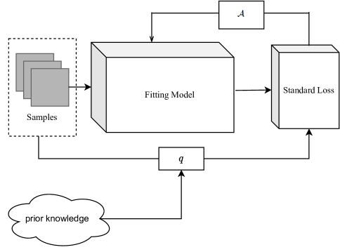
Figure 2: Basic components of GD Learning.

GD Learning aims to estimate the underlying distribution $\bar{q}$, either $\bar{q}_{Y|X}$ or $\bar{q}_{X}$, using an i.i.d. sample set $s$. Therefore we formulate GD Learning into two situations:

• native distribution learning

  $$\min_{f\in\mathcal{F}}\mathbb{E}_{Z\sim\bar{q}}\|\bar{q}-p\|\,\ \mathrm{s.t.}\,\ s=\{z_{i}\}_{i=1}^{n},$$ (17)

  where $p=M(f)$ with $M:\mathcal{F}\to\Delta$, denotes a mapping informed by prior knowledge about distribution $\bar{q}$ to convert parameter $f$ into a probability distribution. When $\bar{q}$ is a PMF over finite support, we set $M(f)=(f)_{\Omega^{*}}^{*}$.

• conditional distribution learning

  $$\min_{f_{x}\in\mathcal{F}}\mathbb{E}_{X\sim\bar{q}_{X}}\|\bar{q}_{Y|x}-p_{Y|x}\|\,\ \mathrm{s.t.}\,\ s=\{z_{i}\}_{i=1}^{n},$$ (18)

  where $p_{Y|x}=M(f_{x})$, and $M$ similarly transforms $f_{x}$ to the corresponding probability distribution. Analogously, when $\bar{q}_{Y|x}$ is a PMF with finite support, $M(f_{x})=(f_{x})_{\Omega^{*}}^{*}$ is adopted.

Our work primarily employs $L_{2}$-norm minimization as the default optimization objective. It is justified to use any norm in finite-dimensional spaces, as the equivalence of different norms ensures that the conclusions derived are invariant to the choice of norm.

Conditional distribution learning is inherently linked to supervised learning. Native distribution learning, on the other hand, aligns with unsupervised learning, as it can be considered a specific case of conditional distribution learning when the input variable $X$ is constant, i.e., $X\sim\delta_{x}$. Thus, our primary focus is conditional distribution learning, and the insights derived can be extended to native distribution learning as well.

We introduce the discrepancy function

$$R_{q_{X}}(p_{Y|x},p^{\prime}_{Y|x})=\mathbb{E}_{X\sim q_{X}}\|p_{Y|x}-p^{\prime}_{Y|x}\|_{2},$$ (19)

which measures the average discrepancy between the conditional distribution $p_{Y|x}$ and $p^{\prime}_{Y|x}$ when the random parameter $X$ is sampled from the distribution $q_{X}$. Then the errors in GD Learning are defined as follows:

1. Learning Error: This error serves as the optimization objective, measuring how well the model approximates the underlying true distribution, denoted by $\|\bar{q}-p\|_{2}$. In conditional distribution learning, we extend this concept to the expected learning error, which is typically denoted as

   $$R_{\bar{q}_{X}}(p_{Y|x},q_{Y|x})=\mathbb{E}_{X\sim\bar{q}_{X}}\|\bar{q}_{Y|x}-p_{Y|x}\|_{2},$$ (20)

   where $\theta$ are the model’s parameters. From the definition, it is evident that the learning error corresponds to the expected risk in the statistical learning framework.

2. Fitting Error: This error measures the model’s performance in fitting the estimator $q$, denoted by $\|q-p\|_{2}$. Similarly, in conditional distribution learning, we define the equivalent concept, the average fitting error, as follows:

   $$R_{\hat{q}_{X}}(q_{Y|x},p_{Y|x})=\mathbb{E}_{X\sim\hat{q}_{X}}\|q_{Y|x}-p_{Y|x}\|_{2}.$$ (21)

   .

3. Sampling Error: This error, denoted by $\|q-\bar{q}\|_{2}$, arises from the finite sample size and serves as a model-independent metric that characterizes the sampled data. For conditional distribution learning, the expected sampling error is defined as follows:

   $$R_{\bar{q}_{X}}(q_{Y|x},\bar{q}_{Y|x})=\mathbb{E}_{X\sim\bar{q}_{X}}\|\bar{q}_{Y|x}-q_{Y|x}\|_{2}.$$ (22)

As shown in Figure 2, GD Learning’s architecture involves four main components: fitting model, standard loss, prior knowledge, and a gradient structure control algorithm (represented by $\mathcal{A}$). The fitting model, a parametric function, is utilized to approximate the target distribution, yielding an estimate of its parameters. In this article, we posit that the models under consideration are differentiable. The estimator $q$ of $\bar{q}$ is generated by combining prior knowledge and sampling instances. To address the appropriate utilization of prior knowledge with a given sample set, we introduce the concept of uncertainty. A comprehensive examination of this concept is presented in Section8. As for the standard loss function and gradient structure control algorithms, which differ from those in the statistical learning framework, we analyze them in a separate usage section later in this paper. For a clearer explanation of the algorithm principle, we use native distribution learning as an illustrative example. As shown in Figure 3, in GD Learning, $q$ serves as a bridge between the unknown true distribution $\bar{q}$ and the model output $p$. The optimization objective $\|p-\bar{q}\|$ can be bounded using the triangular inequality, decomposing it into the fitting error and the sampling error. Consequently, minimizing the sampling and fitting errors can effectively control the learning error. A central aspect of sampling error is the selection of an unbiased estimator $q$ for $\bar{q}$. Although $\hat{q}(z)$ is theoretically sound, in practical scenarios, especially in the case of insufficient samples, techniques like Laplacian smoothing and kernel density estimation (KDE) often yield superior performance. To address this, we propose the principle of minimum uncertainty and utilize it to select $q$. Fitting error optimization is often a non-convex problem, and gradient descent algorithms do not guarantee a global optimal solution. To address this, we propose the gradient structure control algorithm, and demonstrate that by reducing the gradient norm and the distance between the maximum and minimum eigenvalues of the Jacobian matrix of parameters, the parameters can approximate the global optimum.

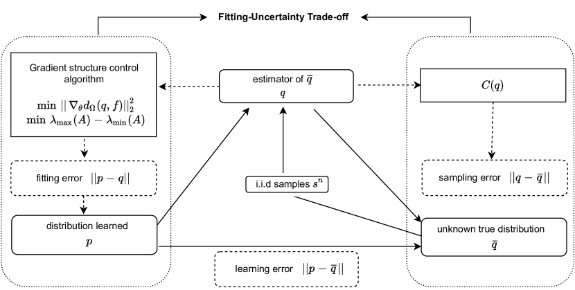
Figure 3: Schematic diagram of GD Learning.

5 Standard loss function

In this section, we formally introduce the concept of a standard loss function and demonstrate its equivalence to both the Fenchel Young loss and Bregman divergence. We then delve into a detailed examination of its fundamental properties. Based on the standard loss function, we introduce the concept of structural error and derive the standard error equality, which serves as a foundation for non-convex optimization in DL learning.

Definition 12 (Standard loss)

A loss function $\ell(q,p):\Delta\times\Delta\to\mathbb{R}^{+}$ is considered a standard loss if it satisfies the following conditions:

• Non-negativity and strict convexity: The loss is non-negative and strictly positive when $q\neq p$, ensuring that it is uniquely minimized when predicting the correct probability $q$.

• Minimization with respect to the true distribution: The expected loss, $\mathbb{E}_{q}\ell(q,p)$, achieves its minimum value when $q=\bar{q}$, expressed as $\bar{q}=\arg\min_{p}\mathbb{E}_{q}\ell(q,p)$.

The uniqueness of the optimal solution allows for a clear connection between the standard loss and the optimization, as it guides the model towards the correct distribution. We establish the equivalence of the standard losses to the Fenchel-Young loss and Bregman divergence in the following theorem.

Theorem 13 (Uniqueness of standard loss)

Given any standard loss $\ell(q,p)$, there exists a strictly convex function $\Omega$ such that $\ell(q,p)=d_{\Omega}(q,p_{\Omega}^{*})=B_{\Omega}(q,p)$, where $d_{\Omega}(q,p_{\Omega}^{*})$ denotes the Fenchel-Young loss, and $B_{\Omega}(q,p)$ represents the Bregman divergence.

The proof of this result is provided in AppendixA.1.

In our study, we represent the standard loss as $d_{\Omega}(q,f_{\theta})$, where $f_{\theta}$ denotes the model parameterized by $\theta$. To maintain generality without compromising clarity, we assume that $d_{\Omega}(q,f_{\theta})$ is continuous and Fréchet differentiable with respect to $\theta$. The standard loss function is a broad concept that encompasses a wide range of commonly used loss functions in statistics and machine learning, as illustrated in Table1.

Table 1: Examples of common loss functions and their corresponding standard forms(Blondel et al., 2019)

Loss	$\mathrm{dom}(\Omega)$	$\Omega(\mu)$	$\hat{y}_{\Omega}(\theta)$	$d_{\Omega}(\theta;y)$
Squared	$\mathbb{R}^{d}$	$\frac{1}{2}\|\mu\|^{2}$	$\theta$	$\frac{1}{2}\|y-\theta\|^{2}$
Perceptron	$\Delta^{|\mathcal{Y}|}$	$0$	$\arg\max(\theta)$	$\max_{i}\theta_{i}-\theta_{k}$
Logistic	$\Delta^{|\mathcal{Y}|}$	$-H(\mu)$	$\mathrm{softmax}(\theta)$	$\log\sum_{i}\exp\theta_{i}-\theta_{k}$
Hinge	$\Delta^{|\mathcal{Y}|}$	$\langle{\mu},{\mathbf{e}_{k}-\mathbf{1}}\rangle$	$\arg\max(\mathbf{1}-\mathbf{e}_{k}+\theta)$	$\max_{i}\leavevmode\nobreak\ [[i\neq k]]+\theta_{i}-\theta_{k}$
Sparsemax	$\Delta^{|\mathcal{Y}|}$	$\frac{1}{2}\|\mu\|^{2}$	$\mathrm{sparsemax}(\theta)$	$\frac{1}{2}\|y-\theta\|^{2}-\frac{1}{2}\|\hat{y}_{\Omega}(\theta)-\theta\|^{2}$
Logistic (one-vs-all)	$[0,1]^{|\mathcal{Y}|}$	$-\sum_{i}H([\mu_{i},1-\mu_{i}])$	$\mathrm{sigmoid}(\theta)$	$\sum_{i}\log(1+\exp(-(2y_{i}-1)\theta_{i}))$

• For multi-class classification, we assume $\mathcal{Y}=\{\mathbf{e}_{i}\}_{i=1}^{d}$ and the ground-truth is $y=\mathbf{e}_{k}$, where $\mathbf{e}_{i}$ denotes a standard basis (”one-hot”) vector.

• For structured classification, we assume that elements of $\mathcal{Y}$ are $d$-dimensional binary vectors with $d\ll|\mathcal{Y}|$, and we denote by $\mathrm{conv}(\mathcal{Y})=\{\mathbb{E}_{p}[Y]\colon p\in\Delta^{\mathcal{Y}}\}$ the corresponding marginal polytope(Wainwright and Jordan, 2008).

• We denote by $H(p):=-\sum_{i}p_{i}\log p_{i}$ the Shannon entropy of a distribution $p\in\Delta^{\mathcal{Y}}$ and $\hat{y}_{\Omega}\in\arg\min_{\mu\in\mathrm{\Omega}}d_{\Omega}(\theta,\mu)$.

Based on the standard loss function, we introduce a novel metric, the structural error, to quantify the directional discrepancy between vectors $e$ and $g$ using the following formulation:

$${T(e,g)}=\frac{1}{2}\min_{a\in\mathbb{R}^{+}}\{\|ae-\frac{g}{a}\|_{2}^{2},\|ae+\frac{g}{a}\|_{2}^{2}\},$$ (23)

where $T(e,g)=0$ iif $\forall i,j,e(i)g(j)=e(j)g(i)$ holds. Notably, $T(e,g)$ is an even function with respect to $g$ by definition, that is, $T(e,g)=T(e,-g)$. When $e$ and $g$ are parameterized by the random variable $X\sim q_{X}$, we define the expected structural error as:

$$\mathbb{E}_{X}T(e_{x},g_{x})=\frac{1}{2}\mathbb{E}_{X}\min_{a\in\mathbb{R}^{+}} \{\|ae_{x}-f_{x}/a\|_{2}^{2}$$ (24)

$$,\|ae_{x}+f_{x}/a\|_{2}^{2}\},$$

and $\mathbb{E}_{X}T(e_{x},g_{x})=0$ iif $\forall i,j,x,g_{x}(i)e_{x}(j)=g_{x}(j)e_{x}(i)$ holds.

We present a theorem that offers a more readily optimized representation of the structural error, as detailed below.

Theorem 14 (structural error equality)

Given functions $e_{x},g_{x}$ parameterized by a random variable $X\sim q_{X}$, the following holds:

$$T(x,f) =\|f\|_{2}\|x\|_{2}-|\langle x,f\rangle|\geq 0,$$ (25)

$$\mathbb{E}_{X}T(e_{x},g_{x}) =\mathbb{E}_{X}\|e_{x}\|_{2}\|g_{x}\|_{2}-\mathbb{E}_{X}|\langle e_{x},g_{x}\rangle|$$

$$\geq 0.$$

The proof of this result is provided in Appendix A.2.

6 Fitting model

In GD Learning, the fitting model serves to estimate the parameters of the target distribution. When the target distribution is discrete, the associated probabilities of support points constitute the parameters. For a continuous target distribution, identifying the specific family of distributions to which it belongs is essential. Consequently, the problem of distribution learning is reformulated as one of estimating the unknown parameters within the identified family of known distributions. It is generally assumed that the fitting model is a universal fitter including NN, Gradient Boosting Decision Tree (GBDT), Support Vector Machine (SVM), XGBoost, etc. NN, especially DNN, is widely used due to their strong fitting ability and good generalization performance. Regarding the fitting ability of NN,the universal approximation theorem (Hornik et al. (1989); Cybenko (1989)) states that a feedforward network with any ”squashing” activation function $\sigma(\cdot)$, such as the logistic sigmoid function, can approximate any Borel measurable function $f(x)$ with any desired non-zero amount of error, provided that the network is given enough hidden layer size $n$. Universal approximation theorems have also been proved for a wider class of activation functions, which includes the now commonly used ReLU (Leshno et al. (1993)). Generally speaking, the more parameters a model has, the stronger its fitting ability. To delve deeper into the influence of fitting models on learning performance beyond their fitting capabilities, we introduce and define the concepts of weak correlation and standard structural models as follows.

Definition 15 (Weak Dependence)

The dependence between random variables is sufficiently weak such that, for the purposes of processing, they can be approximated as independent.

This qualitative definition is crafted to broaden the applicability of conclusions that fulfill independent criteria, thereby making them suitable for a wider array of real-life scenarios. In the fitting model, the dependency of a parameter on others can be assessed by experimentally removing a specific parameter from the model. Specifically, if the model’s output remains essentially unchanged, it indicates that the parameter has weak dependency on other parameters. This weak dependence also contributes to the model’s robustness against noise.

Definition 16 (Standard structural model)

We define a model as a standard structural model when it satisfies the condition $\lambda_{\max}(\nabla_{\theta}f\top\nabla_{\theta}f)=\lambda_{\min}(\nabla_{\theta}f\top\nabla_{\theta}f)$.

A standard structural model has a zero structural error, mathematically expressed as

$$T(e,\nabla_{\theta}f\top\nabla_{\theta}fe)=0.$$ (26)

When the number of parameters is sufficiently large, according to the Universal Approximation Theory, the model possesses the capacity for universal fitting. Upon achieving a perfect fit to the data, the partial derivatives with respect to each parameter are zero. Simultaneously, through the regulation of parameter norms, including techniques such as $L1$ and $L2$ normalization, the parameters exhibit a tendency to converge towards zero. Accordingly, eliminating a particular parameter is equivalent to assigning it a value of zero, and its effect on the final model output is considered negligible. At this point, the inter-parameter dependence is sufficiently weak to allow an approximation of independence. If we additionally posit that the partial derivatives of the output with respect to each parameter are zero-mean random variables that are identically distributed, then the subsequent corollary can be derived from Lemma10.

Corollary 17

When the number of model parameters is sufficiently large, perfectly fits the data, and the partial derivatives of each parameter are distributed according to the same zero-mean distribution, then the model is considered to exhibit a standard structure.

As previously discussed, the impact of the number of parameters on structural error has been examined. We will now elucidate how the model’s architecture also significantly influences the model’s structural error. Firstly, we categorize the model’s parameters into two groups: $\theta=[\theta^{s},\theta^{c}]$, where $\theta^{c}$ represents the set of common parameters shared across each output dimension, and $\theta^{s}$represents the set of unique parameters for each output dimension. Furthermore, we denote the set of self-owned parameters of $f_{i}$ as $\theta^{i}$. Then we have

$$\nabla_{\theta}f_{i} =(\nabla_{\theta^{s}}f_{i},\nabla_{\theta^{c}}f_{i})$$ (27)

$$=(0,\cdots,\nabla_{\theta^{i}}f_{i},0,\cdots,0,\nabla_{\theta^{c}}f_{i}),$$

$$\nabla_{\theta}f_{i}^{\top}\nabla_{\theta}f_{j}=\nabla_{\theta^{c}}f_{i}^{\top}\nabla_{\theta^{c}}f_{j},$$ (28)

$$\nabla_{\theta}f_{i}^{\top}\nabla_{\theta}f_{i}=\nabla_{\theta^{c}}f_{i}^{\top}\nabla_{\theta^{c}}f_{i}+\nabla_{\theta^{i}}f_{i}^{\top}\nabla_{\theta^{i}}f_{i}$$

We assume that $\nabla_{\theta^{i}}f_{i}^{\top}\nabla_{\theta^{i}}f_{i}=a,\forall i$, indicating that the squared norm of the gradient for each $f_{i}$ with respect to its unique parameters $\theta^{i}$ is constant. Consequently, we have $\nabla_{\theta}f^{\top}\nabla_{\theta}f=aI+\epsilon B$, where $\epsilon B_{ij}=\nabla_{\theta^{c}}f_{i}^{\top}\nabla_{\theta^{c}}f_{j}$, and $\lambda_{\max}B=1$. The larger the proportion of self-owned parameters, the greater the value of $a/\epsilon$. Specifically, when $a/\epsilon\gg 1$, the matrix $\nabla_{\theta}f^{\top}\nabla_{\theta}f$ tends to be close to a diagonal matrix. According to Corollary17, if $|\theta^{c}|\gg|f|$ and the model is well-trained, it follows that $\lambda_{\max}(B)\approx\lambda_{\min}(B)$. Therefore, we have $\lambda_{\max}(\nabla_{\theta}f^{\top}\nabla_{\theta}f)=\lambda_{\min}(\nabla_{\theta}f^{\top}\nabla_{\theta}f)$.

The quantity of parameters and the structural design of the model are pivotal in determining the dependencies among parameters. Parameter normalization is a beneficial strategy that ensures the partial derivatives of parameters adhere to a distribution with a zero mean. The application of such techniques can confer standard structural characteristics upon the model. Furthermore, our investigation has revealed that numerous deep learning techniques can be effectively interpreted through the lens of constructing models with standard structural properties.

1. The random initialization of parameters in DNNs(Glorot and Bengio, 2010; He et al., 2015b) ensures that the values of gradient $\nabla_{\theta}f_{i}$ for an untrained model are randomly assigned, and helps to reduce the dependence between parameter gradients, $\nabla_{\theta}f_{i}$ and $\nabla_{\theta}f_{j}$.

2. Gradient-based iterative algorithms typically focus on reducing the magnitude of the gradient, $\|\nabla_{\theta}f_{j}\|$, without altering its direction. This leads to weak dependence between the direction vectors of $\nabla_{\theta}f_{j}$ and $\nabla_{\theta}f_{i}$ for $i\neq j$. Randomly selecting samples in each iteration of stochastic gradient descent (SGD) or batch gradient descent (Batch-GD) leads to a random gradient direction update, thereby enhancing the independence of direction vectors.

3. Dropout(Krizhevsky et al., 2012) ensures that the loss remains relatively constant even when specific nodes in DNNs are temporarily discarded. This effectively reduces the influence of these nodes on other parameters, thereby decreasing parameter dependency.

4. As the number of layers between parameter $\theta_{i}$ and $\theta_{j}$ increases, the dependence between $\nabla_{\theta_{i}}f$ and $\nabla_{\theta_{j}}f$ weakens. With a sufficiently deep DNN, it is justifiable to assume that the majority of the gradients exhibit a high degree of approximate independence.

Collectively, when the parameter count is sufficiently large, these arguments justify the rationale behind modeling the gradients as i.i.d. samples.

7 Gradient structure control algorithm

In this section, we propose a novel gradient structure control algorithm to address the challenges faced by gradient-based optimization methods with non-convex objectives. Specifically, we demonstrate that within the GD Learning framework, reducing the gradient norm and the discrepancy between the maximum and minimum eigenvalues of the Jacobian matrix of parameters ensures convergence to the global optimum. We begin by defining an optimization problem of interest:

$$\min_{\theta}d_{\Omega}(h,f_{\theta}),$$ (29)

where $f_{\theta}$ is continuously Fréchet differentiable with respect to $\theta$, $h$ is the constant vector we aim to fit, and $|h|$ represents its dimensionality.

Introducing $A:=\nabla_{\theta}f^{\top}\nabla_{\theta}f$ as the matrix constructed from the product of the gradient of the function $f$ with respect to the parameters $\theta$ with itself, and $e:=\nabla_{f}d_{\Omega}(h,f)$ representing the gradient of $d_{\Omega}(h,f)$ with respect to $f$, we proceed to present a pivotal theoretical assertion:

Theorem 18 (bound of gradient structure control)

Assuming $\|Ae\|\neq 0$, the following inequality holds:

$$\frac{\|\nabla_{\theta}d_{\Omega}(h,f)\|_{2}^{2}}{\|Ae\|_{2}} \leq\|e\|_{2}\leq\frac{\beta\|e\|_{2}^{2}+\|\nabla_{\theta}d_{\Omega}(h,f)\|_{2}^{2}}{\|Ae\|_{2}},$$ (30)

where $\beta=\frac{(\lambda_{\max}(A)-\lambda_{\min}(A))^{2}}{4(\lambda_{\max}(A)+\lambda_{\min}(A))}$, and $\beta$ is the upper bound of the $T(e,Ax)$.

The proof of this theorem is provided in Appendix A.3.

Based on the established Theorem18, we deduce the following corollaries with additional insights.

Corollary 19 (number of parameters)

1. When $|\theta|<|h|$, we have

   $$\frac{\lambda_{\max}(A)\|x\|_{2}^{2}}{4} \geq\|e\|_{2}\|Ae\|_{2}-\|\nabla_{\theta}d(h,f)\|_{2}^{2}$$ (31)

   $$\geq 0.$$

2. When $A=aI$, it follows that:

   $$\|e\|_{2}\|Ae\|_{2}-\|\nabla_{\theta}d(h,f)\|_{2}^{2}=0.$$ (32)

3. If $|\theta|\gg|h|$, we have

   $$\lim_{|\theta|\to\infty} A=aI,$$ (33)

   $$\lim_{|\theta|\to\infty} \|e\|_{2}\|Ae\|_{2}-\|\nabla_{\theta}d(h,f)\|_{2}^{2}=0,$$

   where $a\in\mathbb{R}^{+}$.

The derivations for these corollaries are presented in Appendix A.4.

These corollaries emphasize the significance of i.i.d. gradients when the number of parameters is large, as it relates to minimizing structural errors in learning. We propose that this also elucidates why first-order optimization methods, such as SGD, can perform effectively in non-convex optimization problems. However, there is a distinction in the theoretical framework: while classical theory posits that the inherent stochasticity serves as an implicit regularization, guiding parameters towards flat plateaus with lower generalization errors, in GD Learning, the inherent stochasticity is used to mitigate structural error in overparameterized models. We define a model $f$ as having good symmetry if the elements of its gradient $\nabla_{\theta}f$ are i.i.d. samples from a distribution with a zero mean. It is evident that an overparameterized model exhibiting such symmetry tends to have zero structural error. Various techniques in deep learning, including SGD, Dropout, random initialization of parameters, deeper networks, and normalizing gradient amplitudes, contribute to this symmetry, ultimately enhancing the learning performance. Therefore, we believe that the ability to reduce structural errors is the main reason why these techniques can improve deep learning performance.

Theorem 18 asserts that minimizing $\|\nabla_{\theta}d_{\Omega}(h,f)\|_{2}^{2}$ and $T(e,Ae)$ results in a decrease in the value of $\|e\|_{2}$, a natural progression that subsequently guides the development of the gradient structure control algorithm. The gradient structure control algorithm is mathematically formulated as:

$$\min_{\theta}\|\nabla_{\theta}d_{\Omega}(h,f)\|_{2}^{2}+\lambda\beta,$$ (34)

where $\lambda$ is a non-negative hyperparameter that weights the bound of the structural error $\beta$. Optimizing this objective above derives the model’s output closer to the desired $q$, guiding the convergence of parameters to the global optimum.

Gradient-based optimization methods, including SGD, Batch-GD, and Newton’s method, primarily focus on minimizing the square $L_{2}$ norm of the gradient, $\|\nabla_{\theta}d(q,f)\|_{2}^{2}$. Alternative methods such as simulated annealing and genetic algorithms can also be employed as complementary strategies to achieve this objective. As for the optimization of $\beta$, we will establish that overparameterization, flat minima, and dynamic isometry are conducive to reducing $\beta$ in the subsequent Section 9.2.

Additionally, considering the model’s expressive capacity, complex models with greater expressive power may have multiple optima where both $|\nabla_{\theta}d_{\Omega}(q,f)|_{2}^{2}=0$ and $\beta=0$ are simultaneously met. This implies that as models grow in complexity, they possess a larger number of potential global optima, which could potentially offer advantages in terms of better fit and adaptability.

8 Bounds of learning error

This section introduces the concept of uncertainty for quantifying the risk introduced by sampling and establishing bounds on the fitting error. Leveraging the triangle inequality, we derive an upper bound for the learning error in GD Learning. Given that the traditional bias-variance trade-off may fall short in fully capturing the behavior of DNNs, we propose a new principle in GD Learning, the fitting-uncertainty trade-off. This principle, derived from the bounds on learning error, offers a new perspective on the relationship between the model’s generalization ability and its fitting power.

We commence by defining generalization error as the absolute discrepancy between the expected loss under the true distribution $\bar{q}$ and its estimator $q$, formalized by:

$$\mathrm{gen}(\bar{q},q,\ell):=|\mathbb{E}_{Z\sim q}\ell(z)-\mathbb{E}_{Z\sim\bar{q}}\ell(z)|,$$ (35)

where $\ell:\mathcal{Z}\to[0,L]$ is a loss function with a known upper bound $L$. To establish a connection between generalization error and KL divergence, we present the following lemma:

Lemma 20

$D_{KL}(q\|\bar{q})\geq\frac{2}{L^{2}}(\mathbb{E}_{q}\ell(z)-\mathbb{E}_{\bar{q}}\ell(z))^{2}$.

The proof of this result is provided in AppendixA.5.

Since $\bar{q}$ is unknown, we model it as a random variable subject to constraints on the i.i.d. sample set $s^{n}$. To formally quantify the uncertainty associated with the sampled data under the estimation $q$, we introduce the quantity $C(q)=\mathbb{E}_{\bar{q}|q}D_{KL}(q\parallel\bar{q})$, where $nq\sim\mathrm{multinomial}(\bar{q})$, and $q$ is absolutely continuous with respect to $\bar{q}$, denoted by $q\ll\bar{q}$.

Subsequently, we delve into the fundamental properties of the uncertainty measure.

Proposition 21 (properties of uncertainty)

The uncertainty possesses the following properties:

• As the sample size escalates, the uncertainty tends asymptotically towards zero:

  $$\lim_{n\to\infty}C(q)=0$$ (36)

• If the sample data is indifferent and all existing constraints are satisfied, a more uniform $q$ implies less uncertainty.

The proof of this result is provided in AppendixA.8.

The principle of maximum entropy posits that the most probable distribution under specified constraints is that with the maximum entropy. Since the Shannon entropy, $H(q)$, is also an indicator of $q$’s uniformity, there exists a certain equivalence between the negative Shannon entropy $-H(q)$ and the uncertainty $C(q)$.

By utilizing uncertainty, we derive upper bounds for both generalization and sampling errors, as established by the subsequent theorems, reflecting the quantitative relationship between these errors and uncertainty.

Theorem 22 (Bound on generalization error)

$$\Pr(\mathrm{gen}(\bar{q},q,\ell)\geq\epsilon)\leq\frac{L^{2}C(q)}{2\epsilon^{2}}.$$ (37)

The proof of this result is provided in AppendixA.6.

Theorem 23

If $\bar{q}$ has finite support points, then we have

$$\|q-\bar{q}\|_{2}^{2} \leq 2D_{KL}(q\|\bar{q})$$ (38)

$$\Pr(\|q-\bar{q}\|_{2} \geq\epsilon)\leq\frac{2C(q)}{\epsilon^{2}}.$$

The proof of this result is provided in AppendixA.7.
Let us define:

$$A_{x}=\nabla_{\theta}f_{x}^{\top}\nabla_{\theta}f_{x},$$ (39)

$$e_{x}=q_{Y|x}-p_{Y|x},$$

$$\mathrm{gen}(\bar{q}_{X},q_{X},\|p_{Y|x}-\bar{q}_{Y|x}\|_{2})=|R_{q_{X}}(p_{Y|x},\bar{q}_{Y|x})-R_{\bar{q}_{X}}(p_{Y|x},\bar{q}_{Y|x})|,$$

then we have the following theorem which provides a bound on the learning error.

Theorem 24 (bound on learning error)

$$R_{\bar{q}_{X}}(p_{Y|x},\bar{q}_{Y|x}) \leq R_{q_{X}}(p_{Y|x},q_{Y|x})+R_{q_{X}}(q_{Y|x},\bar{q}_{Y|x})$$ (40)

$$+\mathrm{gen}(\bar{q}_{X},q_{X},\|p_{Y|x}-\bar{q}_{Y|x}\|_{2}),$$

where

$$R_{q_{X}}(p_{Y|x},q_{Y|x})\leq\mathbb{E}_{X}\frac{2\beta_{x}+\|\nabla_{\theta}d_{\Omega}(q_{x},f_{x})\|_{2}^{2}}{\|A_{x}e_{x}\|_{2}},$$ (41)

$$\Pr(\|q_{Y|x}-\bar{q}_{Y|x}\|_{2}\geq\epsilon)\leq\frac{2C(q_{Y|x})}{\epsilon^{2}},$$

$$\Pr(\mathrm{gen}(\bar{q}_{X},q_{X},\|p_{Y|x}-\bar{q}_{Y|x}\|)\geq\epsilon)\leq\frac{C(q_{X})}{\epsilon^{2}}.$$

The proof of this theorem is provided in Appendix A.9.

In typical deterministic classification scenarios with negligible noise, the label probability distribution conditioned on the feature $x$ is given by $\bar{q}_{Y|x}=\delta_{y}$, where $y$ is the label associated with $x$. Under these conditions, the frequency distribution aligns with the true distribution, resulting in $R_{q_{X}}(\hat{q}_{Y|x},\bar{q}_{Y|x})=0$. The bound of the learning error can then be simplified to

$$R_{\bar{q}_{X}}(p_{Y|x},\bar{q}_{Y|x}) \leq R_{q_{X}}(p_{Y|x},\hat{q}_{Y|x})+\mathrm{gen}(\bar{q}_{X},q_{X},\|p_{Y|x}-\bar{q}_{Y|x}\|)$$ (42)

where the learning error is determined by the fitting error and the uncertainty $C(q_{X})$.

Within the upper bound of the learning error, the terms $\beta_{x}$, $\|\nabla_{\theta}d_{\Omega}(q_{x},f_{x})\|_{2}^{2}$, $C(q_{Y|x})$ and $C(q_{X})$ are relatively manageable. The success of GD Learning heavily relies on the four controllable terms, which are intricately linked to the choice of $q_{X}$ and $q_{Y|x}$. Therefore, the selection of appropriate $q_{X}$ and $q_{Y|x}$ is of paramount significance in GD Learning.

Theorem 21 suggests that when the sample size is significantly large relative to the entropy, fitting error is the dominant factor in learning error. Conversely, uncertainty acts as the dominant factor. Thus, we deduce the following principle for choosing the proper $q$:

Proposition 25 (fitting-uncertainty trade-off)

In scenarios where the sample size is relatively insufficient, uncertainty plays a substantial role in learning errors, favoring the use of $q$ with higher entropy over the frequency distribution $\hat{q}$. As the sample size grows to be sufficiently large, uncertainty becomes negligible, allowing us to approximate $\bar{q}$ by $\hat{q}$.

In other words, higher uncertainty corresponds to lower confidence in the data, and therefore, a greater reliance on prior knowledge. As a result, the emphasis on data fitting should be reduced. Conversely, when uncertainty is low, the data contains almost all the information on the true underlying distribution $\bar{q}$, and the model should strive for a perfect fit on the data. The bias-variance trade-off indicates that as the complexity of the model increases, bias decreases while variance increases. They cannot both disappear and rise simultaneously. However, the results of a series of experiments on DNNs appear to contradict the traditional intuition of a strict trade-off (Neal et al., 2018). Unlike the classic bias-variance trade-off used to describe the characteristics of the model itself, our proposed fitting-uncertainty trade-off describes the relationship between the model and data, as well as how they collectively determine learning errors. Our conclusion is consistent with the formal form of maximum entropy estimation, which suggests that, within the given constraints, objects characterized by higher entropy or those that exhibit a smoother nature are generally more favorable. This principle is exemplified by techniques like label smoothing (Szegedy et al., 2015), and Synthetic Minority Oversampling Technique (SMOTE) (Chawla et al., 2002), which introduce a degree of smoothness into the existing data and yield positive outcomes.

9 Understanding DL from the perspective of GD Learning

9.1 Classification and regression

In this section, we delve into the classification using softmax with cross-entropy loss and regression with mean squared error (MSE) loss. By examining these two fundamental instances, we illustrate the unification of classification and regression tasks within the GD learning framework.

The combination of softmax with cross-entropy is a standard choice to train neural network classifiers. It measures the cross-entropy between the ground truth label and the output of the neural network. The expected cross-entropy loss, denoted by $R(\theta)$, is given by:

$$R(\theta) =-\mathbb{E}_{X\sim q_{X}}\sum_{y\in\mathcal{Y}}q_{Y|x}(y)\log\frac{e^{f_{x}(y)}}{\sum_{y^{\prime}\in\mathcal{Y}}e^{f_{x}(y^{\prime})}}$$ (43)

$$=-\mathbb{E}_{X\sim q_{X}}\langle q_{Y|x},f_{x}\rangle+\mathbb{E}_{X}\log{\sum_{y\in\mathcal{Y}}e^{f_{x}(y)}}$$

where $f_{x}$ is the input to the softmax function. By adding a model-independent item $-H(q_{Y|X})$, we can reformulate $R(\theta)$ into a standard loss function as follows:

$$\mathbb{E}_{X\sim q_{X}}d_{\Omega}(q_{Y|x},f_{x}) =R(\theta)-H(q_{Y|X}),$$ (44)

where $H(q_{Y|X})$ represents the Shannon conditional entropy, $\Omega(q_{Y|x})=D_{KL}(q_{Y|x}\|U)$, and $U$ represents the uniform distribution over $\mathcal{Y}$. Consequently, classification with softmax cross-entropy is a specific instance of GD Learning.

Regression with MSE loss is a superior and fundamental statistical analysis method, due to its high computational efficiency and mathematical interpretability. Assuming that the label $Y$ conditioned on the given feature $x$ follows a multivariate normal distribution, we can express it as:

$$p(y|x)=\frac{1}{(2\pi)^{k/2}|\Sigma|^{1/2}}\exp\left(-\frac{1}{2}(y-{\mu_{x}})^{\top}\Sigma^{-1}(y-{\mu_{x}})\right),$$ (45)

where $k$ is the dimension of $y$, $\Sigma=cI$, and $c\in\mathbb{R}^{+}$. We approximate the Dirac Delta function $\delta_{y}$ by $\lim_{a\to 0^{+}}N(y,aI)$, where $N(y,aI)$ represents the Gaussian distribution. The standard loss is then defined as $d_{\Omega}(q_{Y|x},f_{x})=D_{KL}(q_{Y|x}\|p_{Y|x})$, where $\Omega(q_{Y|x})=D_{KL}(q_{Y|x},U)$, and $U$ is the uniform distribution over $\mathcal{Y}$. This leads to:

$$D_{KL}(\delta_{y}||p_{Y|x}) =\frac{1}{2}[\log\frac{|cI|}{|aI|}-k+(y-{\mu_{x}})^{\top}(y-{\mu_{x}})$$ (46)

$$+\mathrm{trace}\left\{aI\right\}],$$

$$\propto(y-{\mu_{x}})^{\top}(y-{\mu_{x}}).$$

Consequently, the average fitting error can be expressed as:

$$\mathbb{E}_{X} d_{\Omega}(q_{Y|x},f_{x})=\mathbb{E}_{X}[\mathbb{E}_{Y|x}d_{\Omega}(\delta_{y},f_{x})$$ (47)

$$-\mathbb{E}_{Y|x}\Omega(\delta_{y})+\Omega(q_{Y|x})]$$

$$=\mathbb{E}_{X}[\mathbb{E}_{Y|x}D_{KL}(\delta_{y},p_{Y|x})-\mathbb{E}_{Y|x}\Omega(\delta_{y})+\Omega(q_{Y|x})]$$

$$\propto\mathbb{E}_{X}\mathbb{E}_{Y|x}(y-\mu_{x})^{\top}(y-\mu_{x}).$$

Thus, regression with MSE loss is equivalent to GD learning under a Gaussian prior distribution.

9.2 Deep learning from the perspective of GD Learning

In this section, we theoretically analyze the impact of overparameterization, flat minima, and dynamic isometry(Saxe et al., 2013) on learning performance within the GD Learning framework. We demonstrate that flat minima, overparameterization, and dynamic isometry serve as implementation methods of the gradient structure control algorithm, providing a deeper understanding of their roles in deep learning.

First, we establish the following theorem to illustrate that in classification tasks with softmax cross-entropy loss, the largest eigenvalue of the Hessian matrix associated with the loss function is bounded by that of the Gram matrix $A_{x}=\nabla_{\theta}f_{x}^{\top}\nabla_{\theta}f_{x}$, highlighting the relationship between flat minima and structural error minimization.

Lemma 26

Let $A=(a_{ij})_{m\times m}$ be a symmetric matrix. Then we have

$$a_{ii}\leq\lambda_{\max}(A)\leq\mathrm{trace}(A)\leq m\lambda_{\max}(A),\forall i\leq m.$$ (48)

The proof of this result is provided in Appendix A.11.

Lemma 27

Let $A,B$ be non-negative definite matrices. Then we have

$$\lambda_{\min}(A+B) \geq\lambda_{\min}(A)+\lambda_{\min}(B)$$ (49)

$$\lambda_{\max}(A+B) \leq\lambda_{\max}(A)+\lambda_{\max}(B).$$

The proof of this result is provided in Appendix A.10.

Theorem 28

Let us define

$$\mathbb{E}_{X\sim q_{X}}d_{\Omega}(q_{Y|x})=\mathbb{E}_{X\sim q_{X}}D_{KL}(q_{Y|x},p_{Y|x}),$$ (50)

and assume the following equations hold after training:

$$\mathbb{E}_{Y\sim p_{Y|x}}\nabla_{\theta}f_{x}(y)=0,$$ (51)

$$\mathbb{E}_{X\sim q_{X}}\mathbb{E}_{Y\sim q_{Y|x}(y)}\frac{\nabla_{\theta}^{2}p_{Y|x}(y)}{p_{Y|x}(y)}=0.$$

Then we have:

$$\lambda_{\max}(H)\leq\max_{x}\lambda_{\max}(A_{x}),$$ (52)

where $H$ is the Hessian for $\mathbb{E}_{X\sim q_{X}}D_{KL}(q_{Y|x},p_{Y|x})$.

The proof of this result is provided in Appendix A.12.

In other words, when employing softmax cross-entropy loss, which is given by $R(\theta)$, minimizing $\lambda_{\max}(A_{x}),\forall x\in\mathcal{X}$, is equivalent to minimizing $\lambda_{\max}(\nabla^{2}_{\theta}R(\theta))$. When the parameter count $|\theta|$ is less than the cardinality of the label set $\mathcal{Y}$, $A_{x}$ is underdetermined, resulting in a zero minimum eigenvalue, $\lambda_{\min}(A_{x})=0$. In this scenario, referring to Corollary 19 and Theorem 24, the fitting error bound is governed by the parameter $\beta_{x}=\frac{\lambda_{\max}(A_{x})}{4}$, suggesting that minimizing $\lambda_{\max}(A_{x})$ is advantageous in reducing fitting and learning error, aligning with the flat minima theory. Therefore, when applying softmax cross-entropy loss, flat minima can be regarded as an empirical conclusion of the specific case of Theorem 24, which offers a broader perspective on the relationship between learning performance and eigenvalues.

Next, we proceed to investigate the impact of parameter count on learning performance. Theorem 19 indicates that the convergence of structural error to zero is guaranteed as the parameter count increases. In this case, the fitting error can be controlled solely by the norm of gradients. This underlies the abilities of overparameterized models to approximate global optimal solutions for non-convex optimization through gradient-based iterative algorithms, as well as the excellent performance of DNNs.

The dynamic isometry condition posits that a model exhibits favorable properties when the singular value distribution of its input-output Jacobian matrix is nearly uniform around 1. Models that satisfy this condition at initialization are often considered to possess strong characteristics, warranting high expectations for their training outcomes, as demonstrated by empirical evidence across diverse network architectures(Xiao et al., 2018; Chen et al., 2020).

It is evident that, under the dynamic isometry condition, the value of the structural error is suppressed. This is advantageous for reducing fitting errors, as demonstrated by the bound of learning error in Corollary 19. Therefore, GD Learning also provides a theoretical rationale for dynamic isometric initialization.

The preceding analysis reveals that flat minima can be viewed as an optimization technique to mitigate structural errors, while overparameterization can be interpreted as a strategy that reduces structural errors through model architecture. Dynamic isometric initialization, on the other hand, contributes to minimizing structural errors through its initialization approach. Collectively, these well-established phenomena and theories effectively address the core issue of structural error reduction. Hence, we introduce the principle of minimum structural error. The preceding analysis provides a rationale to consider this principle as fundamental to the comprehension of deep learning mechanisms. Furthermore, the definition of structural error suggests that enhancing the orthogonality among gradient vectors and ensuring the modulus values of the constraints are roughly equivalent can effectively reduce structural error. Notably, augmenting the symmetry within the neural network architecture facilitates the attainment of orthogonality among gradients and uniformity in gradient modulus values. Consequently, we speculate that enhancing the symmetry within network architectures, which encompasses strategies such as weight regulation and the normalization of input and intermediate layer features, are practical methods to enforce the minimum structural error principle. The consistency with existing theories and experimental phenomena, as well as the explanatory power of existing theories and phenomena, demonstrate the correctness and effectiveness of our proposed framework.

10 Conclusion

This study introduces a novel theoretical learning framework, GD Learning, which offers a comprehensive perspective on various machine learning and statistical tasks. GD Learning is distinguished by its emphasis on the true underlying distribution, decomposing learning errors into sampling error and fitting errors, revealing the profound influence of the sample set on learning performance. Moreover, the framework significantly incorporates prior knowledge, especially in scenarios characterized by data scarcity measured by uncertainty. We also introduce the gradient structure control algorithm for non-convex optimization objectives, which extends gradient-based methods and establishes an effective bound on learning error under its application. We demonstrate that GD Learning unifies diverse tasks, such as classification, regression, and parameter estimation within a unified theoretical framework. By introducing the principle of minimum structural error, our framework offers clearer insights into the unanswered problems on deep learning, including the roles of flat minima, overparameterization, and dynamical isometry in learning performance, and provides a theoretical explanation for their impact. To address the limitations of the bias-variance trade-off in deep learning, we propose and prove the fitting-uncertainty trade-off theory. It highlights the importance of balancing the fitting error of existing data with the learned distribution’s uncertainty, thus offering a tailored solution for deep learning scenarios. GD Learning is theoretically capable of elucidating the theoretical rationale behind phenomena and offering a more general form. The consistency of our framework with existing theories and experimental phenomena, as well as the explanatory power of existing theories and phenomena, demonstrate the correctness and effectiveness of our proposed framework.

Acknowledgments and Disclosure of Funding

All acknowledgements go at the end of the paper before appendices and references. Moreover, you are required to declare funding (financial activities supporting the submitted work) and competing interests (related financial activities outside the submitted work). More information about this disclosure can be found on the JMLR website.

Appendix A Proofs

A.1 Proof of Theorem 13

Since $\ell(q,p)$ is continuous, Fréchet differentiable, and has a unique minimum value of zero at $p=q$, where its gradient with respect to $p$ vanishes, i.e., $\nabla_{p}\ell(q,q)=0$, we can express this gradient as

$$\nabla_{p}\ell(q,p)=(p-q)^{\top}g(q,p).$$ (53)

Due to the unbiasedness of the minimum value, the expected loss, $\mathbb{E}_{q\sim Q}\ell(q,p)$, is strictly convex, and at its minimum $\bar{q}$, the gradient with respect to $p$ vanishes, i.e., $\nabla_{p}\mathbb{E}_{q\sim Q}\ell(q,\bar{q})=0$, which implies that $\sum_{q\in\mathcal{Q}}Q(q)(\bar{q}-q)^{\top}g(q,\bar{q})=0$, where $q\sim Q$.

Given that $Q(q)$ is an arbitrary distribution function, $g(q,p)$ must be independent of $q$, allowing us to replace $g(q,p)$ by $g(p)$.

Since $\mathbb{E}_{q\sim Q}\ell(q,p)$ is a strictly convex function, its Hessian with respect to $p$ can be derived as:

$$\nabla^{2}_{p}\mathbb{E}_{q\sim Q}\ell(q,p)=\sum_{q\in\mathcal{Q}}Q(q)[g(p)+(p-q)^{\top}\nabla_{p}g(p)].$$ (54)

Simplifying we get:

$$\nabla^{2}_{p}\mathbb{E}_{q\sim Q}\ell(q,p)=g(p)+(p-\bar{q})\nabla_{p}g(p)>0.$$ (55)

The inequality above is derived from the fact that $\nabla^{2}_{p}\mathbb{E}_{q\sim Q}\ell(q,p)$ is strictly convex.

When $p$ is set to $\bar{q}$, we have $\nabla^{2}_{p}\mathbb{E}_{q\sim Q}\ell(q,p)=g(\bar{q})>0$. Since $\bar{q}$ can take any value, it follows that for any arbitrary $p$, we get $g(p)>0$.

Let us define a strictly convex function $\Omega(p)$ with its Hessian matrix given by $\nabla^{2}_{p}\Omega(p)=g(p)$. The gradient of the loss function $\ell(q,p)$ with respect to $p$ can be expressed as follows:

$$\nabla_{p}\ell(q,p) =\nabla^{2}_{p}\Omega(p)(p-q)$$ (56)

$$=\nabla_{p}p_{\Omega}^{*}p-\nabla_{p}p_{\Omega}^{*}q$$

$$=\nabla_{p}(\langle p,p_{\Omega}^{*}\rangle-\Omega(p))-q^{\top}\nabla_{p}p_{\Omega}^{*}$$

$$=\nabla_{p}(\Omega^{*}(p_{\Omega}^{*})-\langle q,p_{\Omega}^{*}\rangle+h(q)).$$

Since $\nabla_{p}\ell(q,q)=0$, we find that $h(q)=\Omega^{*}(q_{\Omega}^{*})-\langle q,q_{\Omega}^{*}\rangle=\Omega(q)$. This leads to the following expression for the loss function: $\ell(q,p)=\Omega^{*}(p_{\Omega}^{*})-\langle q,p_{\Omega}^{*}\rangle+\Omega(q)$. According to the equivalence between Bregman divergence and Fenchel-Young loss 8, the loss function can also be represented as the Bregman divergence with respect to $\Omega$, denoted by $\ell(q,p)=B_{\Omega}(q,p)$.

A.2 Proof of Theorem 14

We introduce a function $F(a)=a^{2}\|x\|_{2}^{2}+\|f\|_{2}^{2}/a^{2}$, where $a\in\mathbb{R}^{+}$. Taking the first and second derivatives of $F(a)$, we get

$$\nabla_{a}F(a) =\frac{d}{da}\left(a^{2}\|x\|_{2}^{2}+\frac{\|f\|_{2}^{2}}{a^{2}}\right)$$ (57)

$$=2a\|x\|_{2}^{2}-\frac{2\|f\|_{2}^{2}}{a^{3}},$$

$$\nabla^{2}_{a}F(a) =\frac{d^{2}}{da^{2}}\left(a^{2}\|x\|_{2}^{2}+\frac{\|f\|_{2}^{2}}{a^{2}}\right)$$

$$=\frac{d}{da}\left(2a\|x\|_{2}^{2}-\frac{2\|f\|_{2}^{2}}{a^{3}}\right)$$

$$=2\|x\|_{2}^{2}+\frac{6\|f\|_{2}^{2}}{a^{4}}.$$

The second derivative is non-negative for all $a>0$. Consequently, $F(a)$ possesses a unique globally minimum, specifically, a value of $\|x\|_{2}\|f\|_{2}$, which is attained at the critical point $a=(\|f\|_{2}^{2}/\|x\|_{2}^{2})^{1/4}$. From the relationships:

$$\|ax-f/a\|_{2}^{2} =\|ax\|_{2}^{2}+\|f/a\|_{2}^{2}-\langle x,f\rangle,$$ (58)

$$\geq\|x\|_{2}\|f\|_{2}-\langle x,f\rangle,$$

$$\|ax+f/a\|_{2}^{2} =\|ax\|_{2}^{2}+\|f/a\|_{2}^{2}+\langle x,f\rangle,$$

$$\geq\|x\|_{2}\|f\|_{2}+\langle x,f\rangle,$$

where the equations hold when $a=(\|f\|_{2}^{2}/\|x\|_{2}^{2})^{1/4}$, we can derive the expression for $T(x,f)$:

$$T(x,f)=\|f\|_{2}\|x\|_{2}-|\langle x,f\rangle|\geq 0,$$ (59)

with equality holding iif $\forall i,j,x_{i}f_{j}=x_{j}f_{i}$. Similarly, for the expected value with respect to $X$, we have

$$\mathbb{E}_{X}T(e_{x},g_{x})=\mathbb{E}_{X}\|e_{x}\|_{2}\|g_{x}\|_{2}-\mathbb{E}_{X}|\langle e_{x},g_{x}\rangle|\geq 0,$$ (60)

equality holds iif $\forall i,j,g_{x}(i)e_{x}(j)=g_{x}(j)e_{x}(i)$.

A.3 Proof of Theorem 18

Let us define:

$$B(a) :=(aI-A/a)$$ (61)

$$\epsilon :=(\lambda_{\max}(A)-\lambda_{\min}(A))/2\lambda_{\max}(A),$$

where $0\leq\epsilon\leq\frac{1}{2}$. The following relationships hold:

$$\lambda_{\min}(B(a)) =\lambda_{\min}(A)/a-a$$ (62)

$$\lambda_{\max}(B(a)) =\lambda_{\max}(A)/a-a$$

$$\lambda_{\max}(B(a)^{\top}B(a)) =\max\{(\lambda_{\max}(A)/a-a)^{2}$$

$$,(a-\lambda_{\min}(A)/a)^{2}\}.$$

If the condition $\lambda_{\max}(A)/a-a\geq a-\lambda_{\min}(A)/a$ holds, the maximum eigenvalue of $B(a)^{\top}B(a)$ is given by:

$$\lambda_{\max}(B(a)^{\top}B(a))=(\lambda_{\max}(A)/a-a)^{2}.$$ (63)

Furthermore, when

$$a=\sqrt{\lambda_{\max}(A)(1-\epsilon)},$$ (64)

$\lambda_{\max}(B(a)^{\top}B(a))$ attains its minimum value, which is

$$\frac{\lambda_{\max}(A)\epsilon^{2}}{1-\epsilon}.$$ (65)

When the inequality $\lambda_{\max}(A)/a-a<a-\lambda_{\min}(A)/a$ holds, then the maximum eigenvalue of $B(a)^{\top}B(a)$ is given by:

$$\lambda_{\max}(B(a)^{\top}B(a))=(a-\lambda_{\min}(A)/a)^{2}.$$ (66)

In the case $a=\sqrt{\lambda_{\max}(A)(1-\epsilon)}$, $\lambda_{\max}(B(a)^{\top}B(a))$ reaches its minimum value, which is also

$$\frac{\lambda_{\max}(A)\epsilon^{2}}{1-\epsilon}.$$ (67)

Since $A$ is a symmetric matrix, we have

$$\lambda_{\max}(A) \geq\lambda_{\min}(A)\geq 0,$$ (68)

$$\min_{a\in\mathbb{R}^{+}}\|ae-Ae/a\|_{2}^{2} \leq\min_{a\in\mathbb{R}^{+}}\|ae+Ae/a\|_{2}^{2}.$$

Consequently, we obtain that:

$$T(e,Ae) =\frac{1}{2}\min_{a\in\mathbb{R}^{+}}\|ae-Ae/a\|_{2}^{2}$$ (69)

$$=\frac{1}{2}\min_{a\in\mathbb{R}^{+}}e^{\top}B(a)^{\top}B(a)e$$

$$\leq\frac{1}{2}\|e\|_{2}^{2}\min_{a\in\mathbb{R}^{+}}\lambda_{\max}(B(a)^{\top}B(a))$$

$$=\frac{1}{2}\|e\|_{2}^{2}\frac{\lambda_{\max}(A)\epsilon^{2}}{1-\epsilon}$$

$$=\frac{(\lambda_{\max}(A)-\lambda_{\min}(A))^{2}\|e\|_{2}^{2}}{4(\lambda_{\max}(A)+\lambda_{\min}(A))}.$$

The last equation is derived by substituting $\epsilon$ with $\frac{1}{2}(1-\frac{\lambda_{\min}(A)}{\lambda_{\max}(A)})$.

Let $\beta=\frac{(\lambda_{\max}(A)-\lambda_{\min}(A))^{2}}{4(\lambda_{\max}(A)+\lambda_{\min}(A))}$, where $\lambda_{\min}(A)\geq 0$, we have $0\leq\beta\leq\frac{\lambda_{\max}}{4}$.

Applying theorem 14, we obtain the following inequality:

$$0 \leq T(e,Ae)$$ (70)

$$=\|e\|_{2}\|Ae\|_{2}-\|\nabla_{\theta}d_{\Omega}(q,f)\|_{2}^{2}$$

$$\leq\beta\|e\|_{2}^{2}.$$

Consequently, we have

$$\frac{\|\nabla_{\theta}d_{\Omega}(q,f)\|_{2}^{2}}{\|Ae\|_{2}}\leq\|e\|_{2}\leq\frac{\beta\|e\|_{2}^{2}+\|\nabla_{\theta}d_{\Omega}(q,f)\|_{2}^{2}}{\|Ae\|_{2}}$$ (71)

A.4 Proof of Corollary 19

When $|\theta|<|h|$, the matrix $A$ is underdetermined, resulting in $\lambda_{\min}(A)=0$. Leveraging Theorem 14, we obtain:

$$\lambda_{\max}(A)\|x\|_{2}^{2}/4\geq T(e,Ae)=\|e\|_{2}\|Ae\|_{2}-\|\nabla_{\theta}F(f)\|_{2}^{2}\geq 0.$$ (72)

In the special case where $A=aI$, the inequality above simplifies to $T(e,Ae)=0$, thus $\|e\|_{2}\|Ae\|_{2}-\|\nabla_{\theta}F(f)\|_{2}^{2}=0$.

When $|\theta|\gg|h|$, based on Corollary 17, we assume that for scenarios where the model is well trained, the elements of $\nabla_{\theta}f$ are drawn as i.i.d. samples from a distribution with zero mean, thus the model is standard structural. Consequently, when $|\theta|$ approaches infinity, we have $\lim_{|\theta|\to\infty}T(e,Ae)=0$. Utilizing equation (72), we obtain

$$\lim_{|\theta|\to\infty}\|e\|_{2}={\|\nabla_{\theta}F(f)\|_{2}^{2}}/\|Ae\|_{2}.$$ (73)

A.5 Proof of Lemma 20

Firstly, let’s derive the upper bound of a as follows:

$$|\mathbb{E}_{q} \ell-\mathbb{E}_{\bar{q}}\ell|=|\sum_{z\in\mathcal{Z}}(q(z)-\bar{q}(z))\ell(z)|$$ (74)

$$=|\sum_{z\in\mathcal{Z}}(\bar{q}(x)-q(x))(\ell(z)-\frac{L}{2})+\frac{L}{2}(\bar{q}(z)-q(z))|$$

$$\leq\sum_{z\in\mathcal{Z}}|\bar{q}(z)-q(z)||\ell(z)-\frac{L}{2}|$$

$$\leq\frac{L}{2}\|q-\bar{q}\|_{1}$$

Employing Pinsker’s inequality (Csiszar, 1967; Kullback, 1967), we have:

$$D_{KL}(q\|\bar{q})\geq\frac{1}{2}\|q-\bar{q}\|_{1}^{2}.$$ (75)

Combining equation (74) and equation (75) gives us:

$$D_{KL}(q\|\bar{q})\geq\frac{2}{L^{2}}|\mathbb{E}_{q}\ell(z)-\mathbb{E}_{\bar{q}}\ell(z)|^{2}$$ (76)

A.6 Proof of Theorem 22

According to Lemma 20, we have

$$D_{KL}(q\|\bar{q})\geq\frac{2}{L^{2}}\mathrm{gen}(\bar{q},q,\ell)^{2},$$ (77)

where $L=\max_{x}\ell(x)$. Consequently, we obtain:

$$\Pr(D_{KL}(q\|\bar{q})\geq t) \geq\Pr(\frac{2}{L^{2}}\mathrm{gen}(\bar{q},q,\ell)^{2}\geq t)$$ (78)

$$=\Pr(\mathrm{gen}(\bar{q},q,\ell)^{2}\geq L^{2}t/2)$$

$$=\Pr(\mathrm{gen}(\bar{q},q,\ell)\geq L\sqrt{t/2}).$$

Let $\epsilon$ be defined as $\epsilon=L\sqrt{t/2}$. By applying lemma 11, we obtain the subsequent inequality:

$$\Pr(\mathrm{gen}(\bar{q},f)\geq\epsilon) \leq\Pr(D_{KL}(q\|\bar{q})\geq\frac{2\epsilon^{2}}{L^{2}})$$ (79)

$$\leq\frac{L^{2}\mathbb{E}_{\bar{q}|q}D_{KL}(q\|\bar{q})}{2\epsilon^{2}}.$$

A.7 Proof of Theorem 23

Let $e$ be a vector of dimension $k$, then we have

$$\|e\|_{1}^{2} =\sum_{i=1}^{k}\sum_{j=1}^{k}\|e(i)\|e(j)\|$$ (80)

$$\geq\sum_{i=1}^{k}\|e(i)\|^{2}$$

$$=\|e\|_{2}^{2}.$$

Employing Pinsker’s inequality (75), we have:

$$D_{KL}(q\|\bar{q})\geq\frac{1}{2}\|\bar{q}-q\|_{1}^{2}.$$ (81)

Since $\bar{q}$ has finite supports, combining the inequality (80) and inequality (81), we have

$$D_{KL}(q\|\bar{q})\geq\frac{1}{2}\|q-\bar{q}\|_{2}^{2}.$$ (82)

Applying lemma 11, we obtain the following result:

$$\Pr(\|q-\bar{q}\|_{2}\geq\epsilon) \leq\Pr(2D_{KL}(q\|\bar{q})\geq\epsilon^{2})$$ (83)

$$\leq\frac{2\mathbb{E}_{\bar{q}|q}D_{KL}(q\|\bar{q})}{\epsilon^{2}}.$$

A.8 Proof of Proposition 21

According to the Bayesian theorem and Sanov’s theorem (Cover, 1999), we have

$$\begin{aligned} &\Pr(\bar{q}|q)={\Pr(q|\bar{q})\Pr(\bar{q})}/{\Pr(q)}\\ &\lim_{n\to\infty}-\frac{1}{n}\log\Pr(q|\bar{q})=D_{KL}(q\|\bar{q}).\end{aligned}$$ (84)

Combining the above equations, as $n$ approaches infinity, we obtain:

$$\lim_{n\to\infty}\Pr(\bar{q}=q|q) =1$$ (85)

$$\lim_{n\to\infty}\mathbb{E}_{\bar{q}|q}D_{KL}(q\|\bar{q}) =0.$$

Now, let’s find the lower bound of $C(q)$:

$$C(q) =-H(q)-\mathbb{E}_{\bar{q}|q}\mathbb{E}_{Z\sim q}\log\bar{q}(z)$$ (86)

$$=-H(q)-\mathbb{E}_{Z\sim q}\mathbb{E}_{\bar{q}|q}\log\bar{q}(z)$$

$$\geq-H(q)-\mathbb{E}_{Z\sim q}\log\mathbb{E}_{\bar{q}|q}\bar{q}(z),$$

where the final inequality is derived from the Jensen’s inequality, as $-\log(\cdot)$ is a convex function. Given that $\sum_{Z}\mathbb{E}_{\bar{q}|q}\bar{q}(z)=1$, we have

$$C(q)\geq D_{KL}(q\|\mathbb{E}_{\bar{q}|q}\bar{q}).$$ (87)

Then the upper bound of $C(q)$ is derived as follows:

$$C(q) =-H(q)-\mathbb{E}_{\bar{q}|q}\mathbb{E}_{Z\sim q}\log\bar{q}(z)$$ (88)

$$=-H(q)+\mathbb{E}_{\bar{q}|q}\mathbb{E}_{Z\sim q}[1+\frac{1-\bar{q}(z)}{\bar{q}(z)}]$$

$$\leq-H(q)+\mathbb{E}_{\bar{q}|q}\mathbb{E}_{Z\sim q}\frac{1-\bar{q}(z)}{\bar{q}(z)},$$

where the final inequality is based on $\log(1+x)\leq x$. Combine the formula (87) and (88), we have

$$D_{KL}(q\|\mathbb{E}_{\bar{q}|q}\bar{q}) \leq C(q)$$ (89)

$$\leq-H(q)+\mathbb{E}_{\bar{q}|q}\mathbb{E}_{Z\sim q}\frac{1-\bar{q}(z)}{\bar{q}(z)}$$

$$\leq H(q)+\mathbb{E}_{\bar{q}|q}\sum_{Z}\frac{q_{\max}}{\bar{q}(z)}-1.$$

Because $\bar{q}$ is an arbitrary distribution on $\mathcal{Z}$, when $n$ is insufficiently large, the conditional probability $\Pr(\bar{q}=q|q)$ fails to approximate 1, causing $\mathbb{E}_{\bar{q}|q}\bar{q}$ to be relatively uniform. Consequently, a more uniform $q$ often implies a smaller lower $D_{KL}(q\|\mathbb{E}_{\bar{q}|q}\bar{q})$, i.e., a smaller bound of $C(q)$. The fact that $q_{\max}$ influences the upper bound also highlights the advantage of a uniform $q$ in minimizing $C(q)$. Thus, under the condition of satisfying existing constraints, a more uniform $q$ implies lower uncertainty.

A.9 Proof of Theorem 24

By employing the triangle inequality of norms, we obtain the following relationship:

$$R_{q_{X}}(p_{Y|x},\bar{q}_{Y|x}) \leq R_{q_{X}}(p_{Y|x},q_{Y|x})+R_{q_{X}}(q_{Y|x},\bar{q}_{Y|x}).$$ (90)

Based on the definition of $\mathrm{gen}(\bar{q}_{X},q_{X},\|p_{Y|x}-\bar{q}_{Y|x}\|_{2})$, we have

$$R_{\bar{q}_{X}}(p_{Y|x},\bar{q}_{Y|x}) \leq R_{q_{X}}(p_{Y|x},\bar{q}_{Y|x})$$ (91)

$$+\mathrm{gen}(\bar{q}_{X},q_{X},\|p_{Y|x}-\bar{q}_{Y|x}\|_{2}).$$

Combining the above inequality and inequality (90), we obtain

$$R_{\bar{q}_{X}}(p_{Y|x},\bar{q}_{Y|x}) \leq R_{q_{X}}(p_{Y|x},q_{Y|x})+R_{q_{X}}(q_{Y|x},\bar{q}_{Y|x})$$ (92)

$$+\mathrm{gen}(\bar{q}_{X},q_{X},\|p_{Y|x}-\bar{q}_{Y|x}\|_{2}).$$

Given that $\|p_{Y|x}-\bar{q}_{Y|x}\|_{2}\leq\sqrt{2}$, by Theorem22, we have

$$\Pr(\mathrm{gen}(\bar{q}_{X},q_{X},\|p_{Y|x}-\bar{q}_{Y|x}\|_{2}\geq\epsilon)\leq\frac{C(q_{X})}{\epsilon^{2}}.$$ (93)

According to Theorem 23, we have:

$$\Pr(\|q_{Y|x}-\bar{q}_{Y|x}\|_{2}\geq\epsilon)\leq\frac{2C(q_{Y|x})}{\epsilon^{2}}.$$ (94)

Invoking Theorem 18, we have:

$$\frac{\|\nabla_{\theta}d_{\Omega}(q_{Y|x},f_{x})\|_{2}^{2}}{\|A_{x}e_{x}\|_{2}}\leq\|e_{x}\|_{2}\leq\frac{2\beta_{x}+\|\nabla_{\theta}d_{\Omega}(q_{Y|x},f_{x})\|_{2}^{2}}{\|A_{x}e_{x}\|_{2}},$$ (95)

where $\beta_{x}=\frac{(\lambda_{\max}(A_{x})-\lambda_{\min}(A_{x}))^{2}}{4(\lambda_{\max}(A_{x})+\lambda_{\min}(A_{x}))}$.

Taking the expectation of the above inequality with respect to $X$, we derive:

$$\mathbb{E}_{X}\frac{\|\nabla_{\theta}d_{\Omega}(q_{x},f_{x})\|_{2}^{2}}{\|A_{x}e_{x}\|_{2}} \leq R_{q_{X}}(p_{Y|x},q_{Y|x})$$ (96)

$$\leq\mathbb{E}_{X}\frac{2\beta_{x}+\|\nabla_{\theta}d_{\Omega}(q_{x},f_{x})\|_{2}^{2}}{\|A_{x}e_{x}\|_{2}}.$$

Combining the inequalities (96),(93),(83), we obtain

$$R_{\bar{q}_{X}}(p_{Y|x},\bar{q}_{Y|x})\leq R_{q_{X}}(p_{Y|x},q_{Y|x})+R_{q_{X}}(q_{Y|x},\bar{q}_{Y|x})$$ (97)

$$+\mathrm{gen}(\bar{q}_{X},q_{X},\|p_{Y|x}-\bar{q}_{Y|x}\|_{2}),$$

$$\mathbb{E}_{X}\frac{\|\nabla_{\theta}d_{\Omega}(q_{x},f_{x})\|_{2}^{2}}{\|A_{x}e_{x}\|_{2}}\leq R_{q_{X}}(p_{Y|x},q_{Y|x})$$

$$\leq\mathbb{E}_{X}\frac{2\beta_{x}+\|\nabla_{\theta}d_{\Omega}(q_{x},f_{x})\|_{2}^{2}}{\|A_{x}e_{x}\|_{2}},$$

$$\Pr(\mathrm{gen}(\bar{q}_{X},q_{X},\|p_{Y|x}-\bar{q}_{Y|x}\|_{2}\geq\epsilon)\leq\frac{C(q_{X})}{\epsilon^{2}},$$

$$\Pr(\|q_{Y|x}-\bar{q}_{Y|x}\|_{2}\geq\epsilon)\leq\frac{2C(q_{Y|x})}{\epsilon^{2}}.$$

A.10 Proof of Lemma 27

Since $x^{\top}Ax\geq\lambda_{\min}(A)x^{\top}x$, it follows that

$$x^{\top}(A-\lambda_{\min}(A)I)x\geq 0,$$ (98)

and $A-\lambda_{\min}(A)I$ is a non-negative definite matrix. Therefore, we have

$$A-\lambda_{\min}(A)I\succeq 0$$ (99)

$$B-\lambda_{\min}(B)I\succeq 0$$

$$A-\lambda_{\min}(A)I+B-\lambda_{\min}(B)I\succeq 0.$$

Let $x^{\prime}$ satisfy the equality $(A+B)x^{\prime}=\lambda_{\min}(A+B)x^{\prime}$, then we have

$$(A- \lambda_{\min}(A)I+B-\lambda_{\min}(B)I)x^{\prime}$$ (100)

$$=(\lambda_{\min}(A+B)-\lambda_{\min}(A)-\lambda_{\min}(B))x^{\prime}.$$

Therefore $\lambda_{\min}(A+B)-\lambda_{\min}(A)-\lambda_{\min}(B)$ is the eigenvalue of $A-\lambda_{\min}(A)I+B-\lambda_{\min}(B)I$. Since $A-\lambda_{\min}(A)I+B-\lambda_{\min}(B)I$ is a non-negative definite matrix, thus we have $\lambda_{\min}(A+B)-\lambda_{\min}(A)-\lambda_{\min}(B)\geq 0$.

Because $x^{\top}A\leq\lambda_{\max}(A)x^{\top}x$, then $x^{\top}(A-\lambda_{\max}(A)I)x\leq 0$, thus $\lambda_{\max}(A)I-A$ is a non-negative definite matrix. Analogously, we can obtain $\lambda_{\max}(A+B)-\lambda_{\max}(A)-\lambda_{\max}(B)\leq 0$.

A.11 Proof of Lemma 26

Given a symmetric matrix $A=(a_{ij})_{m\times m}$, we know that $\lambda_{\min}(A)\geq 0$. Since the sum of eigenvalues is equal to $\mathrm{trace}(A)$, we have

$$\lambda_{\max}(A)\leq\mathrm{trace}(A)\leq m\lambda_{\max}(A).$$ (101)

According to the Courant-Fisher min-max theorem, the maximum eigenvalue is given by:

$$\lambda_{\max}(A)=\max_{x\in\mathbb{R}^{m},\|x\|=1}x^{\top}Ax.$$ (102)

Let $e_{i}$ be a standard basis (”one-hot”) vector. Then we have

$$a_{ii}=e_{i}^{\top}Ae_{i}\leq\lambda_{\max}(A)$$ (103)

A.12 Proof of Theorem 28

Given the relationship: $\mathbb{E}_{X\sim q_{X}}d_{\Omega}(q_{Y|x},f_{x})=\mathbb{E}_{X\sim q_{X}}D_{KL}(q_{Y|x}\|p_{Y|x})$, we can deduce $p_{Y|x}(y)=\frac{e^{f_{x}(y)}}{Z_{x}}$, $Z_{x}$ is the partition function, defined as $Z_{x}=\sum_{y\in\mathcal{Y}}e^{f_{x}(y)}$. Consequently, the gradient of the log-probability with respect to the model parameter $\theta$ decomposes as follows:

$$\nabla_{\theta}\log p_{Y|x}(y)=\nabla_{\theta}f_{x}(y)-\nabla_{\theta}\log Z_{x},$$ (104)

The second gradient term, $\nabla_{\theta}\log Z_{x}$ can be rewritten as an expected value, as follows:

$$\nabla_{\theta}\log Z_{x} =Z_{x}^{-1}\nabla_{\theta}\sum_{y\in\mathcal{Y}}e^{f_{x}(y)}$$ (105)

$$=Z_{x}^{-1}\sum_{y\in\mathcal{Y}}e^{f_{x}(y)}\nabla_{\theta}f_{x}(y)$$

$$=\mathbb{E}_{Y\sim p_{Y|x}}\nabla_{\theta}f_{x}(y).$$

According to the above equality, we have

$$\mathbb{E}_{Y\sim q_{Y|x}}\left\{\nabla_{\theta}\log p_{Y|x}(y)\right\}\left\{\nabla_{\theta}\log p_{Y|x}(y)\right\}^{\top}$$ (106)

$$=\mathbb{E}_{Y\sim q_{Y|x}}\{\nabla_{\theta}f_{x}(y)-\nabla_{\theta}\log Z_{x}\}\{\nabla_{\theta}f_{x}(y)-\nabla_{\theta}\log Z_{x}\}^{\top}$$

$$=\mathbb{E}_{Y\sim q_{Y|x}}\{\nabla_{\theta}f_{x}(y)\nabla_{\theta}f_{x}(y)^{\top}\}$$

$$-2\nabla_{\theta}\log Z_{x}\mathbb{E}_{Y\sim q_{Y|x}}\nabla_{\theta}f_{x}(y)+\nabla_{\theta}\log Z_{x}\nabla_{\theta}\log Z_{x}^{\top}$$

$$=\mathbb{E}_{Y\sim q_{Y|x}}\{\nabla_{\theta}f_{x}(y)\nabla_{\theta}f_{x}(y)^{\top}\}+F_{x}$$

where

$$F_{x}=-2\nabla_{\theta}\log Z_{x}\mathbb{E}_{Y\sim q_{Y|x}}\nabla_{\theta}f_{x}(y)+\nabla_{\theta}\log Z_{x}\nabla_{\theta}\log Z_{x}^{\top}.$$ (107)

The Hessian for $D_{KL}(q_{Y|x},p_{Y|x})$ is equal to compute with the second derivative of negative log-likelihood $-\log p_{Y|x}(y)$, which can be expressed as:

$$\nabla^{2}_{\theta}D_{KL}(q_{Y|x},p_{Y|x})=\mathbb{E}_{Y\sim q_{Y|x}}[-\nabla^{2}_{\theta}\log p_{Y|x}(y)].$$ (108)

Next, we expand the second derivative of it as follows:

$$- \nabla_{\theta}^{2}\log p_{Y|x}(y)=-\nabla_{\theta}\left[\frac{\nabla_{\theta}p_{Y|x}(y)}{p_{Y|x}(y)}\right]$$ (109)

$$=-\frac{p_{Y|x}(y)\nabla_{\theta}^{2}p_{Y|x}(y)-\left\{\nabla_{\theta}p_{Y|x}(y)\right\}\left\{\nabla_{\theta}p_{Y|x}(y)\right\}^{\top}}{p_{Y|x}(y)^{2}}$$

$$=-\frac{\nabla_{\theta}^{2}p_{Y|x}(y)}{p_{Y|x}(y)}+\left\{\frac{\nabla_{\theta}p_{Y|x}(y)}{p_{Y|x}(y)}\right\}\left\{\frac{\nabla_{\theta}p_{Y|x}(y)}{p_{Y|x}(y)}\right\}^{\top}$$

$$=-\frac{\nabla_{\theta}^{2}p_{Y|x}(y)}{p_{Y|x}(y)}+\left\{\nabla_{\theta}\log p_{Y|x}(y)\right\}\left\{\nabla_{\theta}\log p_{Y|x}(y)\right\}^{\top}.$$

Then, we apply this expanded second derivative to (108) which can be restated as follows:

$$\nabla^{2}_{\theta}D_{KL}(q_{Y|x},p_{Y|x})=\mathbb{E}_{Y\sim q_{Y|x}(y)}\left[-\frac{\nabla_{\theta}^{2}p_{Y|x}(y)}{p_{Y|x}(y)}\right]$$ (110)

$$+\mathbb{E}_{Y\sim q_{Y|x}(y)}\left[\left\{\nabla_{\theta}\log p_{Y|x}(y)\right\}\left\{\nabla_{\theta}\log p_{Y|x}(y)\right\}^{\top}\right]$$

$$=C_{x}+B_{x}+F_{x}.$$

where

$$B_{x} =\mathbb{E}_{Y\sim p_{Y|x}}\nabla_{\theta}f_{x}(y)\nabla_{\theta}f_{x}(y)^{\top},$$ (111)

$$C_{x} =\mathbb{E}_{Y\sim q_{Y|x}(y)}\left[-\frac{\nabla_{\theta}^{2}p_{Y|x}(y)}{p_{Y|x}(y)}\right].$$

Since $\nabla_{\theta}f_{x}(y)\nabla_{\theta}f_{x}(y)^{\top}$ is a matrix of rank 1, its eigenvalues are

$$\lambda_{\max}(\nabla_{\theta}f_{x}(y)\nabla_{\theta}f_{x}(y)^{\top}) =\nabla_{\theta}f_{x}(y)^{\top}\nabla_{\theta}f_{x}(y)$$ (112)

$$\lambda_{\min}(\nabla_{\theta}f_{x}(y)\nabla_{\theta}f_{x}(y)^{\top}) =0$$

According to Lemma 27, we can bound the extreme eigenvalues of $B_{x}$ as follows:

$$\lambda_{\max}(B_{x}) \leq\mathbb{E}_{Y\sim p_{Y|x}}\lambda_{\max}(\nabla_{\theta}f_{x}(y)\nabla_{\theta}f_{x}(y)^{\top})$$ (113)

$$\leq\max_{y}\lambda_{\max}(\nabla_{\theta}f_{x}(y)\nabla_{\theta}f_{x}(y)^{\top})$$

$$=\max_{y}\nabla_{\theta}f_{x}(y)^{\top}\nabla_{\theta}f_{x}(y)$$

$$\lambda_{\min}(B_{x}) \geq\mathbb{E}_{Y\sim p_{Y|x}}\lambda_{\min}(\nabla_{\theta}f_{x}(y)\nabla_{\theta}f_{x}(y)^{\top})$$

$$\geq\min_{y}\lambda_{\min}(\nabla_{\theta}f_{x}(y)\nabla_{\theta}f_{x}(y)^{\top})$$

$$=0.$$

Because $A_{x}=\nabla_{\theta}f_{x}^{\top}\nabla_{\theta}f_{x}$ is a symmetric matrix, according to the inequality (113) and lemma26, we have:

$$\lambda_{\max}(B_{x})\leq\max_{y}\nabla_{\theta}f_{x}(y)^{\top}\nabla_{\theta}f_{x}(y) \leq\lambda_{\max}(A_{x}).$$ (114)

The Hessian for $\mathbb{E}_{X\sim q_{X}}D_{KL}(q_{Y|x},p_{Y|x})$ can be expressed as:

$$H=\mathbb{E}_{X\sim q_{X}}B_{x}+\mathbb{E}_{X\sim q_{X}}C_{x}+\mathbb{E}_{X\sim q_{X}}F_{x}.$$ (115)

Since

$$\mathbb{E}_{Y\sim p_{Y|x}}\nabla_{\theta}f_{x}(y)=0,$$ (116)

$$\mathbb{E}_{X\sim q_{X}}\mathbb{E}_{Y\sim q_{Y|x}(y)}\frac{\nabla_{\theta}^{2}p_{Y|x}(y)}{p_{Y|x}(y)}=0,$$

, we obtain

$$H =\mathbb{E}_{X\sim q_{X}}B_{x},$$ (117)

$$\lambda_{\max}(H) \leq\max_{x}\lambda_{\max}(B_{x})\leq\max_{x}\lambda_{\max}(A_{x})$$

Remainder omitted in this sample. See http://www.jmlr.org/papers/ for full paper.

References

- Aldrich (1997) John Aldrich. R.a. fisher and the making of maximum likelihood 1912-1922. Statistical Science, 12:162–176, 1997. URL https://api.semanticscholar.org/CorpusID:53120959.
- Allen-Zhu et al. (2018) Zeyuan Allen-Zhu, Yuanzhi Li, and Zhao Song. A convergence theory for deep learning via over-parameterization. ArXiv, abs/1811.03962, 2018. URL https://api.semanticscholar.org/CorpusID:53250107.
- Amari (2016) Shun-ichi Amari. Information geometry and its applications, volume 194. Springer, 2016.
- Arjevani and Field (2022) Yossi Arjevani and Michael Field. Annihilation of spurious minima in two-layer relu networks. ArXiv, abs/2210.06088, 2022. URL https://api.semanticscholar.org/CorpusID:252846371.
- Bai and Yin (1993) Z. D. Bai and Y. Q. Yin. Limit of the smallest eigenvalue of a large dimensional sample covariance matrix. Annals of Probability, 21:1275–1294, 1993. URL https://api.semanticscholar.org/CorpusID:120161816.
- Barron (1993) Andrew R. Barron. Universal approximation bounds for superpositions of a sigmoidal function. IEEE Trans. Inf. Theory, 39:930–945, 1993. URL https://api.semanticscholar.org/CorpusID:15383918.
- Bartlett and Mendelson (2003) Peter L. Bartlett and Shahar Mendelson. Rademacher and gaussian complexities: Risk bounds and structural results. J. Mach. Learn. Res., 3:463–482, 2003. URL https://api.semanticscholar.org/CorpusID:463216.
- Belkin et al. (2018a) Mikhail Belkin, Daniel J. Hsu, Siyuan Ma, and Soumik Mandal. Reconciling modern machine-learning practice and the classical bias–variance trade-off. Proceedings of the National Academy of Sciences, 116:15849 – 15854, 2018a. URL https://api.semanticscholar.org/CorpusID:198496504.
- Belkin et al. (2018b) Mikhail Belkin, Alexander Rakhlin, and A. Tsybakov. Does data interpolation contradict statistical optimality? ArXiv, abs/1806.09471, 2018b. URL https://api.semanticscholar.org/CorpusID:49412723.
- Blondel et al. (2019) Mathieu Blondel, André F. T. Martins, and Vlad Niculae. Learning with fenchel-young losses. ArXiv, abs/1901.02324, 2019. URL https://api.semanticscholar.org/CorpusID:57721258.
- Bousquet and Elisseeff (2002) Olivier Bousquet and André Elisseeff. Stability and generalization. Journal of Machine Learning Research, 2:499–526, 2002. URL https://api.semanticscholar.org/CorpusID:1157797.
- Chaudhari and Soatto (2017) Pratik Chaudhari and Stefano Soatto. Stochastic gradient descent performs variational inference, converges to limit cycles for deep networks. 2018 Information Theory and Applications Workshop (ITA), pages 1–10, 2017. URL https://api.semanticscholar.org/CorpusID:3515208.
- Chawla et al. (2002) N. Chawla, K. Bowyer, Lawrence O. Hall, and W. Philip Kegelmeyer. Smote: Synthetic minority over-sampling technique. ArXiv, abs/1106.1813, 2002. URL https://api.semanticscholar.org/CorpusID:1554582.
- Chen et al. (2020) Zhaodong Chen, Lei Deng, Bangyan Wang, Guoqi Li, and Yuan Xie. A comprehensive and modularized statistical framework for gradient norm equality in deep neural networks. IEEE Transactions on Pattern Analysis and Machine Intelligence, 44:13–31, 2020. URL https://api.semanticscholar.org/CorpusID:209531864.
- Chizat and Bach (2018) Lénaïc Chizat and Francis R. Bach. On the global convergence of gradient descent for over-parameterized models using optimal transport. ArXiv, abs/1805.09545, 2018. URL https://api.semanticscholar.org/CorpusID:43945764.
- Chizat et al. (2018) Lénaïc Chizat, Edouard Oyallon, and Francis R. Bach. On lazy training in differentiable programming. In Neural Information Processing Systems, 2018. URL https://api.semanticscholar.org/CorpusID:189928159.
- Choromańska et al. (2014) Anna Choromańska, Mikael Henaff, Michaël Mathieu, Gérard Ben Arous, and Yann LeCun. The loss surfaces of multilayer networks. In International Conference on Artificial Intelligence and Statistics, 2014. URL https://api.semanticscholar.org/CorpusID:2266226.
- Cover (1999) Thomas M Cover. Elements of information theory. John Wiley & Sons, 1999.
- Csiszar (1967) I. Csiszar. Information-type measures of difference of probability distributions and indirect observations. Studia . Math. Hungar, 2, 1967.
- Cybenko (1989) George V. Cybenko. Approximation by superpositions of a sigmoidal function. Mathematics of Control, Signals and Systems, 2:303–314, 1989. URL https://api.semanticscholar.org/CorpusID:3958369.
- Dauphin et al. (2014) Yann Dauphin, Razvan Pascanu, Çaglar Gülçehre, Kyunghyun Cho, Surya Ganguli, and Yoshua Bengio. Identifying and attacking the saddle point problem in high-dimensional non-convex optimization. ArXiv, abs/1406.2572, 2014. URL https://api.semanticscholar.org/CorpusID:11657534.
- Dinh et al. (2016) Laurent Dinh, Jascha Sohl-Dickstein, and Samy Bengio. Density estimation using real nvp. arXiv preprint arXiv:1605.08803, 2016.
- Dinh et al. (2017) Laurent Dinh, Razvan Pascanu, Samy Bengio, and Yoshua Bengio. Sharp minima can generalize for deep nets. In International Conference on Machine Learning, 2017. URL https://api.semanticscholar.org/CorpusID:7636159.
- Dreyfus (1962) Stuart E. Dreyfus. The numerical solution of variational problems. Journal of Mathematical Analysis and Applications, 5:30–45, 1962. URL https://api.semanticscholar.org/CorpusID:120388484.
- Du et al. (2018) Simon Shaolei Du, Xiyu Zhai, Barnabás Póczos, and Aarti Singh. Gradient descent provably optimizes over-parameterized neural networks. ArXiv, abs/1810.02054, 2018. URL https://api.semanticscholar.org/CorpusID:52920808.
- Freedman and Diaconis (1981) David Freedman and Persi Diaconis. On the histogram as a density estimator: L 2 theory. Zeitschrift für Wahrscheinlichkeitstheorie und verwandte Gebiete, 57(4):453–476, 1981.
- Ge et al. (2015) Rong Ge, Furong Huang, Chi Jin, and Yang Yuan. Escaping from saddle points - online stochastic gradient for tensor decomposition. ArXiv, abs/1503.02101, 2015. URL https://api.semanticscholar.org/CorpusID:11513606.
- Geiger et al. (2019) Mario Geiger, Arthur Jacot, Stefano Spigler, Franck Gabriel, Levent Sagun, Stéphane d’Ascoli, Giulio Biroli, Clément Hongler, and Matthieu Wyart. Scaling description of generalization with number of parameters in deep learning. Journal of Statistical Mechanics: Theory and Experiment, 2020, 2019. URL https://api.semanticscholar.org/CorpusID:57573772.
- Glorot and Bengio (2010) Xavier Glorot and Yoshua Bengio. Understanding the difficulty of training deep feedforward neural networks. In International Conference on Artificial Intelligence and Statistics, 2010. URL https://api.semanticscholar.org/CorpusID:5575601.
- Griewank and Walther (2000) Andreas Griewank and Andrea Walther. Evaluating derivatives - principles and techniques of algorithmic differentiation, second edition. In Frontiers in applied mathematics, 2000. URL https://api.semanticscholar.org/CorpusID:35253217.
- Hald (1999) Anders Hald. On the history of maximum likelihood in relation to inverse probability and least squares. Statistical Science, 14:214–222, 1999. URL https://api.semanticscholar.org/CorpusID:123501415.
- Hall et al. (2004) Peter Hall, Jeff Racine, and Qi Li. Cross-validation and the estimation of conditional probability densities. Journal of the American Statistical Association, 99(468):1015–1026, 2004.
- Hanin and Sellke (2017) Boris Hanin and Mark Sellke. Approximating continuous functions by relu nets of minimal width. ArXiv, abs/1710.11278, 2017. URL https://api.semanticscholar.org/CorpusID:1681235.
- Härdle et al. (2004) Wolfgang Härdle, Marlene Müller, Stefan Sperlich, Axel Werwatz, et al. Nonparametric and semiparametric models, volume 1. Springer, 2004.
- Hardt et al. (2015) Moritz Hardt, Benjamin Recht, and Yoram Singer. Train faster, generalize better: Stability of stochastic gradient descent. ArXiv, abs/1509.01240, 2015. URL https://api.semanticscholar.org/CorpusID:49015.
- He et al. (2015a) Kaiming He, X. Zhang, Shaoqing Ren, and Jian Sun. Deep residual learning for image recognition. 2016 IEEE Conference on Computer Vision and Pattern Recognition (CVPR), pages 770–778, 2015a. URL https://api.semanticscholar.org/CorpusID:206594692.
- He et al. (2015b) Kaiming He, X. Zhang, Shaoqing Ren, and Jian Sun. Delving deep into rectifiers: Surpassing human-level performance on imagenet classification. 2015 IEEE International Conference on Computer Vision (ICCV), pages 1026–1034, 2015b. URL https://api.semanticscholar.org/CorpusID:13740328.
- Hoeffding (1994) Wassily Hoeffding. Probability inequalities for sums of bounded random variables. The collected works of Wassily Hoeffding, pages 409–426, 1994.
- Hornik et al. (1989) Kurt Hornik, Maxwell B. Stinchcombe, and Halbert L. White. Multilayer feedforward networks are universal approximators. Neural Networks, 2:359–366, 1989. URL https://api.semanticscholar.org/CorpusID:2757547.
- Huber (1964) Peter J. Huber. Robust estimation of a location parameter. Annals of Mathematical Statistics, 35:492–518, 1964. URL https://api.semanticscholar.org/CorpusID:121252793.
- Huber (1973) Peter J. Huber. Robust regression: Asymptotics, conjectures and monte carlo. Annals of Statistics, 1:799–821, 1973. URL https://api.semanticscholar.org/CorpusID:123395408.
- ichi Funahashi (1989) Ken ichi Funahashi. On the approximate realization of continuous mappings by neural networks. Neural Networks, 2:183–192, 1989. URL https://api.semanticscholar.org/CorpusID:10203109.
- Jacot et al. (2018) Arthur Jacot, Franck Gabriel, and Clément Hongler. Neural tangent kernel: Convergence and generalization in neural networks. ArXiv, abs/1806.07572, 2018. URL https://api.semanticscholar.org/CorpusID:49321232.
- Jastrzebski et al. (2017) Stanislaw Jastrzebski, Zachary Kenton, Devansh Arpit, Nicolas Ballas, Asja Fischer, Yoshua Bengio, and Amos J. Storkey. Three factors influencing minima in sgd. ArXiv, abs/1711.04623, 2017. URL https://api.semanticscholar.org/CorpusID:7311295.
- Jentzen et al. (2018) Arnulf Jentzen, Benno Kuckuck, Ariel Neufeld, and Philippe von Wurstemberger. Strong error analysis for stochastic gradient descent optimization algorithms. Ima Journal of Numerical Analysis, 2018. URL https://api.semanticscholar.org/CorpusID:53603316.
- Kawaguchi (2016) Kenji Kawaguchi. Deep learning without poor local minima. ArXiv, abs/1605.07110, 2016. URL https://api.semanticscholar.org/CorpusID:1605269.
- Kawaguchi et al. (2017) Kenji Kawaguchi, Leslie Pack Kaelbling, and Yoshua Bengio. Generalization in deep learning. ArXiv, abs/1710.05468, 2017. URL https://api.semanticscholar.org/CorpusID:3520119.
- Kelley (1960) Henry J. Kelley. Gradient theory of optimal flight paths. ARS Journal, 30:947–954, 1960. URL https://api.semanticscholar.org/CorpusID:121072881.
- Keskar et al. (2016) Nitish Shirish Keskar, Dheevatsa Mudigere, Jorge Nocedal, Mikhail Smelyanskiy, and Ping Tak Peter Tang. On large-batch training for deep learning: Generalization gap and sharp minima. ArXiv, abs/1609.04836, 2016. URL https://api.semanticscholar.org/CorpusID:5834589.
- Kidger and Lyons (2019) Patrick Kidger and Terry Lyons. Universal approximation with deep narrow networks. ArXiv, abs/1905.08539, 2019. URL https://api.semanticscholar.org/CorpusID:160009610.
- Kiefer and Wolfowitz (1952) J. Kiefer and Jacob Wolfowitz. Stochastic estimation of the maximum of a regression function. Annals of Mathematical Statistics, 23:462–466, 1952. URL https://api.semanticscholar.org/CorpusID:122078986.
- Kingma et al. (2016) Durk P Kingma, Tim Salimans, Rafal Jozefowicz, Xi Chen, Ilya Sutskever, and Max Welling. Improved variational inference with inverse autoregressive flow. Advances in neural information processing systems, 29, 2016.
- Krizhevsky et al. (2012) Alex Krizhevsky, Ilya Sutskever, and Geoffrey E. Hinton. Imagenet classification with deep convolutional neural networks. Communications of the ACM, 60:84 – 90, 2012. URL https://api.semanticscholar.org/CorpusID:195908774.
- Kullback (1967) Solomon Kullback. A lower bound for discrimination information in terms of variation (corresp.). IEEE Trans. Inf. Theory, 13:126–127, 1967. URL https://api.semanticscholar.org/CorpusID:206729100.
- Larochelle and Murray (2011) Hugo Larochelle and Iain Murray. The neural autoregressive distribution estimator. In Proceedings of the fourteenth international conference on artificial intelligence and statistics, pages 29–37. JMLR Workshop and Conference Proceedings, 2011.
- Lee et al. (2016) J. Lee, Max Simchowitz, Michael I. Jordan, and Benjamin Recht. Gradient descent only converges to minimizers. In Annual Conference Computational Learning Theory, 2016. URL https://api.semanticscholar.org/CorpusID:5378616.
- Lee et al. (2019) J. Lee, Ioannis Panageas, Georgios Piliouras, Max Simchowitz, Michael I. Jordan, and Benjamin Recht. First-order methods almost always avoid strict saddle points. Mathematical Programming, 176:311 – 337, 2019. URL https://api.semanticscholar.org/CorpusID:126527837.
- Leshno et al. (1993) Moshe Leshno, V. Ya. Lin, Allan Pinkus, and Shimon Schocken. Original contribution: Multilayer feedforward networks with a nonpolynomial activation function can approximate any function. Neural Networks, 6:861–867, 1993. URL https://api.semanticscholar.org/CorpusID:206089312.
- Lewicki and Marino (2003) Grzegorz Lewicki and Giuseppe Marino. Approximation by superpositions of a sigmoidal function. Zeitschrift Fur Analysis Und Ihre Anwendungen, 22:463–470, 2003. URL https://api.semanticscholar.org/CorpusID:16135755.
- Lewkowycz et al. (2020) Aitor Lewkowycz, Yasaman Bahri, Ethan Dyer, Jascha Narain Sohl-Dickstein, and Guy Gur-Ari. The large learning rate phase of deep learning: the catapult mechanism. ArXiv, abs/2003.02218, 2020. URL https://api.semanticscholar.org/CorpusID:211989826.
- Li et al. (2020) Jiajin Li, Anthony Man-Cho So, and Wing-Kin Ma. Understanding notions of stationarity in nonsmooth optimization: A guided tour of various constructions of subdifferential for nonsmooth functions. IEEE Signal Processing Magazine, 37:18–31, 2020. URL https://api.semanticscholar.org/CorpusID:221568212.
- MacKay (2003) David JC MacKay. Information theory, inference and learning algorithms. Cambridge university press, 2003.
- McLachlan et al. (2019) Geoffrey J McLachlan, Sharon X Lee, and Suren I Rathnayake. Finite mixture models. Annual review of statistics and its application, 6:355–378, 2019.
- Meeker et al. (2022) William Q Meeker, Luis A Escobar, and Francis G Pascual. Statistical methods for reliability data. John Wiley & Sons, 2022.
- Mei et al. (2018) Song Mei, Andrea Montanari, and Phan-Minh Nguyen. A mean field view of the landscape of two-layer neural networks. Proceedings of the National Academy of Sciences of the United States of America, 115:E7665 – E7671, 2018. URL https://api.semanticscholar.org/CorpusID:4932688.
- Mukherjee et al. (2006) Sayan Mukherjee, Partha Niyogi, Tomaso Poggio, and Ryan Rifkin. Learning theory: stability is sufficient for generalization and necessary and sufficient for consistency of empirical risk minimization. Advances in Computational Mathematics, 25:161–193, 2006.
- Murphy (2022) Kevin P Murphy. Probabilistic machine learning: an introduction. MIT press, 2022.
- Nagarajan and Kolter (2019) Vaishnavh Nagarajan and J. Zico Kolter. Uniform convergence may be unable to explain generalization in deep learning. In Neural Information Processing Systems, 2019. URL https://api.semanticscholar.org/CorpusID:61153527.
- Nakkiran et al. (2019) Preetum Nakkiran, Gal Kaplun, Yamini Bansal, Tristan Yang, Boaz Barak, and Ilya Sutskever. Deep double descent: where bigger models and more data hurt. Journal of Statistical Mechanics: Theory and Experiment, 2021, 2019. URL https://api.semanticscholar.org/CorpusID:207808916.
- Neal et al. (2018) Brady Neal, Sarthak Mittal, Aristide Baratin, Vinayak Tantia, Matthew Scicluna, Simon Lacoste-Julien, and Ioannis Mitliagkas. A modern take on the bias-variance tradeoff in neural networks. arXiv preprint arXiv:1810.08591, 2018.
- Nemirovski et al. (2008) Arkadi Nemirovski, Anatoli B. Juditsky, Guanghui Lan, and Alexander Shapiro. Robust stochastic approximation approach to stochastic programming. SIAM J. Optim., 19:1574–1609, 2008. URL https://api.semanticscholar.org/CorpusID:268069803.
- Papamakarios et al. (2017) George Papamakarios, Theo Pavlakou, and Iain Murray. Masked autoregressive flow for density estimation. Advances in neural information processing systems, 30, 2017.
- Parzen (1962) Emanuel Parzen. On estimation of a probability density function and mode. The annals of mathematical statistics, 33(3):1065–1076, 1962.
- Poole et al. (2016) Ben Poole, Subhaneil Lahiri, Maithra Raghu, Jascha Narain Sohl-Dickstein, and Surya Ganguli. Exponential expressivity in deep neural networks through transient chaos. In Neural Information Processing Systems, 2016. URL https://api.semanticscholar.org/CorpusID:9408079.
- Rahman et al. (2008) SM Mahbubur Rahman, M Omair Ahmad, and MNS Swamy. Bayesian wavelet-based image denoising using the gauss–hermite expansion. IEEE Transactions on Image Processing, 17(10):1755–1771, 2008.
- Rezende and Mohamed (2015) Danilo Rezende and Shakir Mohamed. Variational inference with normalizing flows. In International conference on machine learning, pages 1530–1538. PMLR, 2015.
- Robbins (1951) Herbert E. Robbins. A stochastic approximation method. Annals of Mathematical Statistics, 22:400–407, 1951. URL https://api.semanticscholar.org/CorpusID:16945044.
- Rumelhart et al. (1986) David E. Rumelhart, Geoffrey E. Hinton, and Ronald J. Williams. Learning representations by back-propagating errors. Nature, 323:533–536, 1986. URL https://api.semanticscholar.org/CorpusID:205001834.
- Saxe et al. (2013) Andrew M. Saxe, James L. McClelland, and Surya Ganguli. Exact solutions to the nonlinear dynamics of learning in deep linear neural networks. CoRR, abs/1312.6120, 2013. URL https://api.semanticscholar.org/CorpusID:17272965.
- Scott (1979) David W Scott. On optimal and data-based histograms. Biometrika, 66(3):605–610, 1979.
- Silverman (2018) Bernard W Silverman. Density estimation for statistics and data analysis. Routledge, 2018.
- Sirignano and Spiliopoulos (2018) Justin A. Sirignano and Konstantinos V. Spiliopoulos. Mean field analysis of neural networks: A central limit theorem. Stochastic Processes and their Applications, 2018. URL https://api.semanticscholar.org/CorpusID:88523128.
- Sivia and Skilling (2006) Devinderjit Sivia and John Skilling. Data analysis: a Bayesian tutorial. OUP Oxford, 2006.
- Sturges (1926) Herbert A Sturges. The choice of a class interval. Journal of the american statistical association, 21(153):65–66, 1926.
- Szegedy et al. (2015) Christian Szegedy, Vincent Vanhoucke, Sergey Ioffe, Jonathon Shlens, and Zbigniew Wojna. Rethinking the inception architecture for computer vision. 2016 IEEE Conference on Computer Vision and Pattern Recognition (CVPR), pages 2818–2826, 2015. URL https://api.semanticscholar.org/CorpusID:206593880.
- Valiant (1984) Leslie G Valiant. A theory of the learnable. Communications of the ACM, 27(11):1134–1142, 1984.
- Vapnik and Alexey (1971) Vladimir N Vapnik and Y Alexey. Chervonenkis. on the uniform convergence of relative frequencies of events to their probabilities. Theory of Probability and its Applications, 16(2):264–280, 1971.
- Wainwright and Jordan (2008) Martin J. Wainwright and Michael I. Jordan. Graphical models, exponential families, and variational inference. Found. Trends Mach. Learn., 1:1–305, 2008. URL https://api.semanticscholar.org/CorpusID:207178945.
- Wu (2021) Yuhai Wu. Statistical learning theory. Technometrics, 41:377–378, 2021. URL https://api.semanticscholar.org/CorpusID:28637672.
- Xiao et al. (2018) Lechao Xiao, Yasaman Bahri, Jascha Narain Sohl-Dickstein, Samuel S. Schoenholz, and Jeffrey Pennington. Dynamical isometry and a mean field theory of cnns: How to train 10, 000-layer vanilla convolutional neural networks. ArXiv, abs/1806.05393, 2018. URL https://api.semanticscholar.org/CorpusID:49208780.
- Xu and Mannor (2010) Huan Xu and Shie Mannor. Robustness and generalization. Machine Learning, 86:391 – 423, 2010. URL https://api.semanticscholar.org/CorpusID:254739858.
- Yun et al. (2018) Chulhee Yun, Suvrit Sra, and Ali Jadbabaie. Small nonlinearities in activation functions create bad local minima in neural networks. In International Conference on Learning Representations, 2018. URL https://api.semanticscholar.org/CorpusID:52893515.
- Zhang et al. (2016) Chiyuan Zhang, Samy Bengio, Moritz Hardt, Benjamin Recht, and Oriol Vinyals. Understanding deep learning requires rethinking generalization. ArXiv, abs/1611.03530, 2016. URL https://api.semanticscholar.org/CorpusID:6212000.
- Zhang et al. (2021) Chiyuan Zhang, Samy Bengio, Moritz Hardt, Benjamin Recht, and Oriol Vinyals. Understanding deep learning (still) requires rethinking generalization. Communications of the ACM, 64:107 – 115, 2021. URL https://api.semanticscholar.org/CorpusID:231991101.
- Zhang et al. (2023) Jingwei Zhang, Tongliang Liu, and Dacheng Tao. Going deeper, generalizing better: An information-theoretic view for deep learning. IEEE transactions on neural networks and learning systems, PP, 2023. URL https://api.semanticscholar.org/CorpusID:260954258.
- Zou et al. (2018) Difan Zou, Yuan Cao, Dongruo Zhou, and Quanquan Gu. Stochastic gradient descent optimizes over-parameterized deep relu networks. ArXiv, abs/1811.08888, 2018. URL https://api.semanticscholar.org/CorpusID:53752874.