Phase-Subtractive Interference and Noise-Resistant Quantum Imaging with Two Undetected Photons

Abstract

We present a quantum interference phenomenon in which four-photon quantum states generated by two independent sources are used to create a two-photon interference pattern without detecting two of the photons. Contrary to the common perception, the interference pattern can be made fully independent of phases acquired by the photons detected to construct it. However, it still contains information about spatially dependent phases acquired by the two undetected photons. This phenomenon can also be observed with fermionic particles. We show that the phenomenon can be applied to develop an interferometric, quantum phase imaging technique that is immune to uncontrollable phase fluctuations in the interferometer and allows image acquisition without detecting the photons illuminating the object.

The principle of quantum superposition, when applied to two-particle systems, yields much richer phenomena than can be observed in single-particle systems. One “mind-boggling” example Greenberger et al. (1993) is interference by path identity of undetected photons Hochrainer et al. (2022), which was first reported by Zou, Wang and Mandel (ZWM) in the early 1990’s Zou et al. (1991); Wang et al. (1991). ZWM created a superposition of the origin of a photon pair and then controlled the interference of one of the photons by path identity of its partner photon. A counter-intuitive fact is that the resulting single-photon interference pattern can be manipulated by interacting with the partner photon which is never detected. Conventional interference by path identity relies on sources that emit coherently, i.e., sources that are not independent. We show that if independent quantum sources are used, an even more counter-intuitive and unusual interference phenomenon emerges. This phenomenon is a manifestation of the four-particle superposition principle and promises a significant advancement in the field of quantum imaging.

We consider a four-photon state generated by two independent quantum sources and show that two-photon interference patterns with unique properties can be created by path identity of two undetected photons. In standard two-particle interference experiments Horne et al. (1989), phase differences associated with the two detected particles get added with the same sign when acquired in the way shown in Fig. 1a. All reported two-particle interference effects obtained by path identity of undetected photons also display the same property Lahiri (2018); Qian et al. (2023). In contrast, the phases of the two detected particles get added with opposite signs in the interference phenomenon reported by us (Fig. 1b). We show by considering multi-mode photonic states that this fact can be used to develop a highly phase-stable interferometer, which produces interferograms that do not depend on the tunable interferometric phase but retain the information of any spatially dependent phase introduced to the undetected photons.

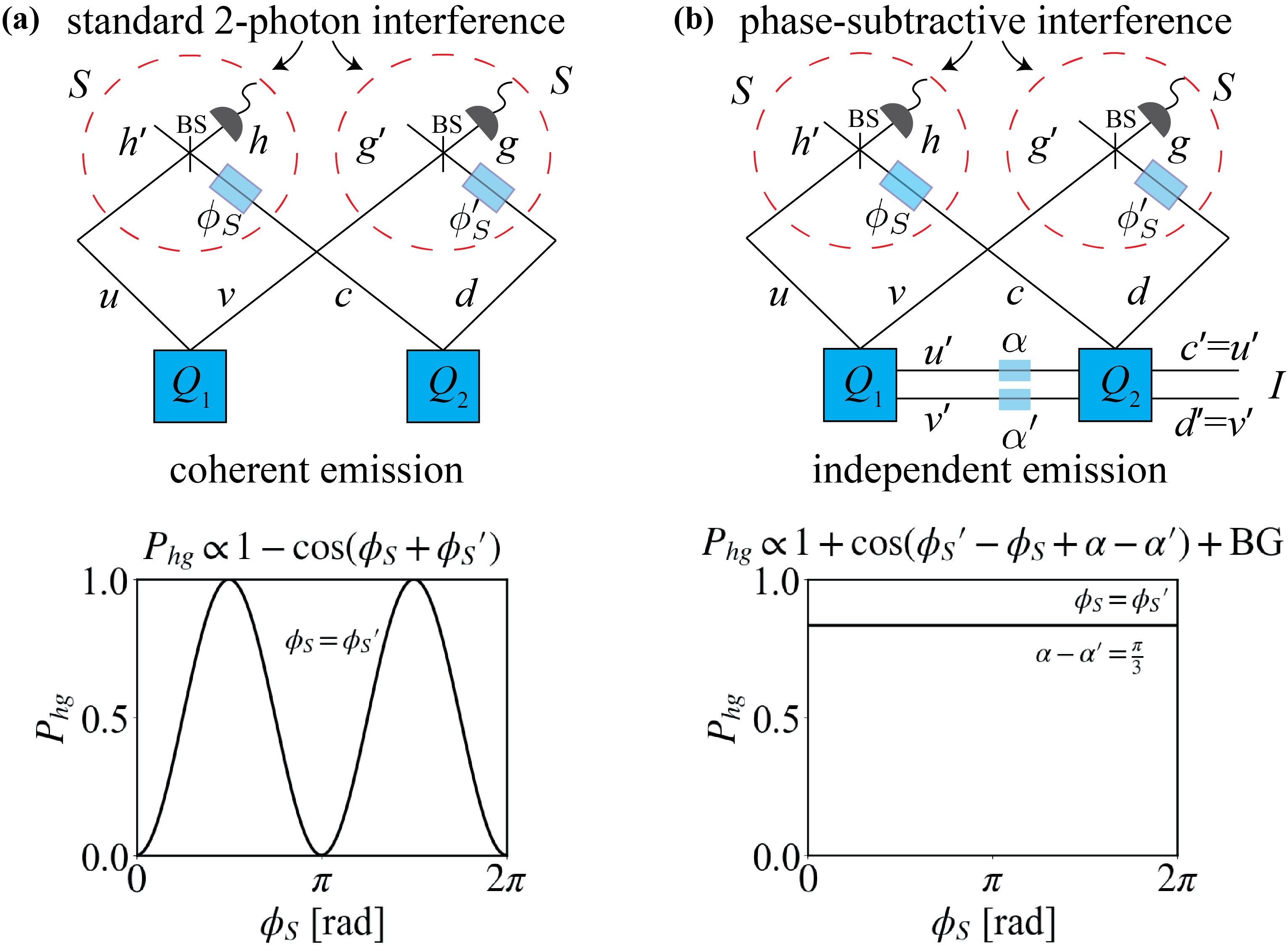
Figure 1: (a) Standard two-particle interference. Sources $Q_{1}$ and $Q_{2}$ coherently emit a pair of identical particles ($S$). The coincidence counting rate ($P_{hg}$) at beamsplitter outputs $g$ and $h$ varies sinusoidally with $\phi_{S}+\phi_{S}^{\prime}$. (b) Phase-subtractive two-photon interference by path identity. $Q_{1}$ and $Q_{2}$ are independent sources emitting two pairs of particles. A pair is made of particles $S$ and $I$. Two-particle interference at $g$ and $h$ is observed by detecting $S$-particles when path identity is employed using $I$-particles, i.e., when paths $u^{\prime}$ and $v^{\prime}$ are made identical with paths $c^{\prime}$ and $d^{\prime}$. The coincidence counting rate varies sinusoidally with $\phi_{S}-\phi_{S}^{\prime}$ and also contains information of phases $\alpha$ and $\alpha^{\prime}$ acquired by undetected particles. The interference pattern is independent of phases acquired by detected particles when $\phi_{S}=\phi_{S}^{\prime}$. (BG: background.)

Conventional interference by path identity has led to the development of a unique imaging technique, namely quantum imaging with undetected photons (QIUP) Lemos et al. (2014); Lahiri et al. (2015); Viswanathan et al. (2021); Kviatkovsky et al. (2022); Lemos et al. (2022). This technique allows one to image an object without detecting photons that interacted with it. Consequently, QIUP allows one to determine optical properties of an object (e.g., absorption profile, phase profile, refractive index) in spectral ranges for which adequate detectors are not available. However, QIUP is vulnerable to uncontrollable random fluctuations of the interferometric phase (phase noise) that arise due to the instability of the interferometer. Therefore, the photon acquisition time in QIUP cannot be long. Furthermore, if the phase noise destroys the interference pattern, QIUP becomes inapplicable. Recently, a noise-resistant interferometric phase imaging (NRIPI) technique has been introduced Szuniewicz et al. (2023); Thekkadath et al. (2023), which is inspired by interference of light from independent quantum sources Pfleegor and Mandel (1967); Mandel (1983); Ou (1997, 2007). However, NRIPI must detect photons that interact with the object and therefore is inapplicable to spectral ranges where adequate detectors are not available. Here, we show that the interference phenomenon reported by us can be applied to develop a phase imaging technique which is immune to phase noise, allows arbitrarily long photon acquisition time, and can acquire images at wavelengths for which no detectors are available.

Let us begin by recollecting some basic features of a standard two-particle interference (Fig. 1a). We consider two coherently and non-simultaneously emitting sources, $Q_{1}$ and $Q_{2}$, each of which can generate a pair of identical particles ($S$). Suppose now that $Q_{1}$ can emit the particle-pair into paths (modes) $u$ and $v$, and $Q_{2}$ can emit them into paths $c$ and $d$. Paths $u$ and $c$ are combined by a beamsplitter with outputs $h$ and $h^{\prime}$. The tunable phase difference between paths $u$ and $c$ is denoted by $\phi_{S}$. Likewise, paths $v$ and $d$ are superposed with phase difference $\phi_{S}^{\prime}$ and corresponding beamsplitter outputs are $g$ and $g^{\prime}$. The probability of coincidence detection of two $S$-particles at $h$ and $g$ gives the well-known expression of a two-particle interference pattern sup :

$$P_{hg}\propto 1-\cos(\phi_{S}+\phi_{S}^{\prime}).$$ (1)

We note that phases $\phi_{S}$ and $\phi_{S}^{\prime}$ got added with the same sign. Such phases also get added in the same manner in conventional two-particle interference by path identity Lahiri (2018); Qian et al. (2023).

Let us now consider a scenario illustrated by Fig. 1b. In this case, four-particle states are generated by double emission of a particle pair. We assume that the two particles forming a pair are, in general, different and denote them by $S$ and $I$. We consider two independent sources, $Q_{1}$ and $Q_{2}$, each of which are capable of both single and double production of the particle pair. $Q_{1}$ can emit a pair of particles into a pair of paths $(u,u^{\prime})$ or $(v,v^{\prime})$. $Q_{2}$ can emit a pair into a pair of paths $(c,c^{\prime})$ or $(d,d^{\prime})$. We assume that paths $u$, $v$, $c$, and $d$ can only be occupied by particle $S$, whereas particle $I$ can only be in paths $u^{\prime}$, $v^{\prime}$, $c^{\prime}$, and $d^{\prime}$. Paths of $S$-particles emerging from the two sources are combined by beamsplitters in the same manner as in the standard two-particle interference discussed above. We are again interested in the probability of coincidence detection of two $S$-particles at $g$ and $h$. However, in the present case (Fig. 1b), particle $I$ is not detected and no further postselection is considered.

There are four possible ways in which a coincidence detection at $g$ and $h$ can occur (Fig. 1b): (1) A double-pair production occurs in $Q_{1}$ creating the state $|S_{u},I_{u^{\prime}},S_{v},I_{v^{\prime}}\rangle_{1}$, where $|S_{u},I_{u^{\prime}},S_{v},I_{v^{\prime}}\rangle_{1}=|S_{u}\rangle_{1}|I_{u^{\prime}}\rangle_{1}|S_{v}\rangle_{1}|I_{v^{\prime}}\rangle_{1}$ and $|S_{u}\rangle_{1}$ denotes a single $S$-particle that is emitted from $Q_{1}$ and in path $u$, etc. (2) A double-pair production occurs in $Q_{2}$ creating the state $|S_{c},I_{c^{\prime}},S_{d},I_{d^{\prime}}\rangle_{2}$. (3) Simultaneous single-pair productions occur at sources $Q_{1}$ and $Q_{2}$ and the resulting state is $|S_{u},I_{u^{\prime}}\rangle_{1}|S_{d},I_{d^{\prime}}\rangle_{2}$. (4) Simultaneous single-pair productions occur at sources $Q_{1}$ and $Q_{2}$ and the resulting state is $|S_{v},I_{v^{\prime}}\rangle_{1}|S_{c},I_{c^{\prime}}\rangle_{2}$.

The two sources are mutually independent, i.e., they cannot emit coherently (Fig. 1b). This fact can be analytically represented by introducing a random (stochastic) phase difference, $\widetilde{\Theta}$, between the two-particle state (equivalently, field) generated by $Q_{1}$ and that by $Q_{2}$. This random phase difference must obey the conditions

$$\langle\exp[i(\widetilde{\Theta}+\phi)]\rangle=\langle\cos(\widetilde{\Theta}+\phi)\rangle=\langle\sin(\widetilde{\Theta}+\phi)\rangle=0,$$ (2)

where $\phi$ is an arbitrary phase and the angular brackets represent averaged value. The quantum state, which contributes to two-photon coincidence detection at $h$ and $g$, can now be expressed as (dropping the normalization coefficient)

$$|\psi\rangle =|S_{u},I_{u^{\prime}},S_{v},I_{v^{\prime}}\rangle_{1}+e^{2i\widetilde{\Theta}}|S_{c},I_{c^{\prime}},S_{d},I_{d^{\prime}}\rangle_{2}$$

$$+e^{i\widetilde{\Theta}}\big{[}|S_{u},I_{u^{\prime}}\rangle_{1}|S_{d},I_{d^{\prime}}\rangle_{2}+|S_{v},I_{v^{\prime}}\rangle_{1}|S_{c},I_{c^{\prime}}\rangle_{2}\big{]}.$$ (3)

Note that states like $|2S_{u}\rangle_{1}|2I_{u^{\prime}}\rangle_{1}$ can be created in a bosonic system but not in a fermionic system. Since such states do not contribute to coincidence counts at $g$ and $h$, Eq. (Phase-Subtractive Interference and Noise-Resistant Quantum Imaging with Two Undetected Photons) applies to both bosonic and fermionic systems.

We now apply path identity Hochrainer et al. (2022): paths of $I$-particles (bosonic or fermionic) from $Q_{1}$ are sent through $Q_{2}$ and aligned with paths of $I$-particles originating from $Q_{2}$ (Fig. 1b), i.e., paths of $I$-particles from the two sources are made identical. Consequently, quantum fields (annihilation operators) corresponding to $I$-particles generated by $Q_{1}$ and $Q_{2}$ become related by $\hat{a}_{I_{2}}(c^{\prime})=e^{i\alpha}\hat{a}_{I_{1}}(u^{\prime})$ and $\hat{a}_{I_{2}}(d^{\prime})=e^{i\alpha^{\prime}}\hat{a}_{I_{1}}(v^{\prime})$. Here, $\alpha$ and $\alpha^{\prime}$ are phases introduced to paths $u^{\prime}$ and $v^{\prime}$, respectively, between the two sources. Since $\hat{a}^{\dagger}_{I_{1}}(u^{\prime})|\text{vac}\rangle\equiv|I_{u^{\prime}}\rangle_{1}$ etc., the path identity implies the following simultaneous relations involving kets: $|I_{c^{\prime}}\rangle_{2}=\exp(-i\alpha)|I_{u^{\prime}}\rangle_{1}$ and $|I_{d^{\prime}}\rangle_{2}=\exp(-i\alpha^{\prime})|I_{v^{\prime}}\rangle_{1}$. Using these relations, we reduce Eq. (Phase-Subtractive Interference and Noise-Resistant Quantum Imaging with Two Undetected Photons) to

$$|\psi\rangle=|I_{u^{\prime}},I_{v^{\prime}}\rangle_{1}\otimes\big{\{}|S_{u},S_{v}\rangle_{1}+e^{i(2\widetilde{\Theta}-\alpha-\alpha^{\prime})}|S_{c},S_{d}\rangle_{2}$$

$$+e^{i\widetilde{\Theta}}\big{[}e^{-i\alpha}|S_{u}\rangle_{1}|S_{d}\rangle_{2}+e^{-i\alpha^{\prime}}|S_{v}\rangle_{1}|S_{c}\rangle_{2}\big{]}\big{\}}.$$ (4)

Equation (Phase-Subtractive Interference and Noise-Resistant Quantum Imaging with Two Undetected Photons) represents the quantum state generated by two independent sources before beamsplitters in Fig. 1b.

The field of $S$-particles (bosonic or fermionic) at the detectors placed at beamsplitter-outputs $h$ and $g$ are given by $\hat{a}_{S}(h)\propto\hat{a}_{S_{1}}(u)+ie^{i\phi_{S}}\hat{a}_{S_{2}}(c)$ and $\hat{a}_{S}(g)\propto\hat{a}_{S_{1}}(v)+ie^{i\phi_{S}^{\prime}}\hat{a}_{S_{2}}(d)$, respectively. The probability of coincidence detection of two $S$-particles at $g$ and $h$ is given by $P_{hg}=\langle\psi|\hat{a}^{\dagger}_{S}(h)\hat{a}^{\dagger}_{S}(g)\hat{a}_{S}(g)\hat{a}_{S}(h)|\psi\rangle$. Using Eqs. (2) and (Phase-Subtractive Interference and Noise-Resistant Quantum Imaging with Two Undetected Photons), we find that

$$P_{hg}\propto 1+\frac{1}{2}\cos(\phi_{S}^{\prime}-\phi_{S}+\alpha-\alpha^{\prime}).$$ (5)

Equation (5) corresponds to interference of two $S$-particles enabled by path identity of two undetected $I$-particles. It can be readily checked that the state given by Eq. (Phase-Subtractive Interference and Noise-Resistant Quantum Imaging with Two Undetected Photons), which is obtained without path identity, does not lead to any interference effect. The visibility of the interference pattern given by Eq. (5) is less than unity because four-particle states emitted individually by each source do not interfere resulting in background. We observe that in Eq. (5), phases $\phi_{S}$ and $\phi_{S}^{\prime}$ got added with opposite signs in striking contrast to standard two-particle interference [Eq. (1)] and conventional two-particle interference by path identity Lahiri (2018); Qian et al. (2023). Therefore, if $\phi_{S}=\phi_{S}^{\prime}$, the interference pattern becomes independent of phases gained by detected particles (Fig. 1b, bottom). Furthermore, if $\alpha\neq\alpha^{\prime}$, the two-particle interference pattern contains information of phases introduced to particles that were never detected to construct the interference pattern (Fig. 1b, bottom). We call such an interference phase-subtractive interference by path identity (PSIPI).

We now show that PSIPI can be realized using photonic states generated by spontaneous parametric down-conversion (SPDC) in nonlinear crystals and that the realization leads to a highly phase-stable interferometer which can be immediately applied to quantum imaging. We neglect losses for simplicity.

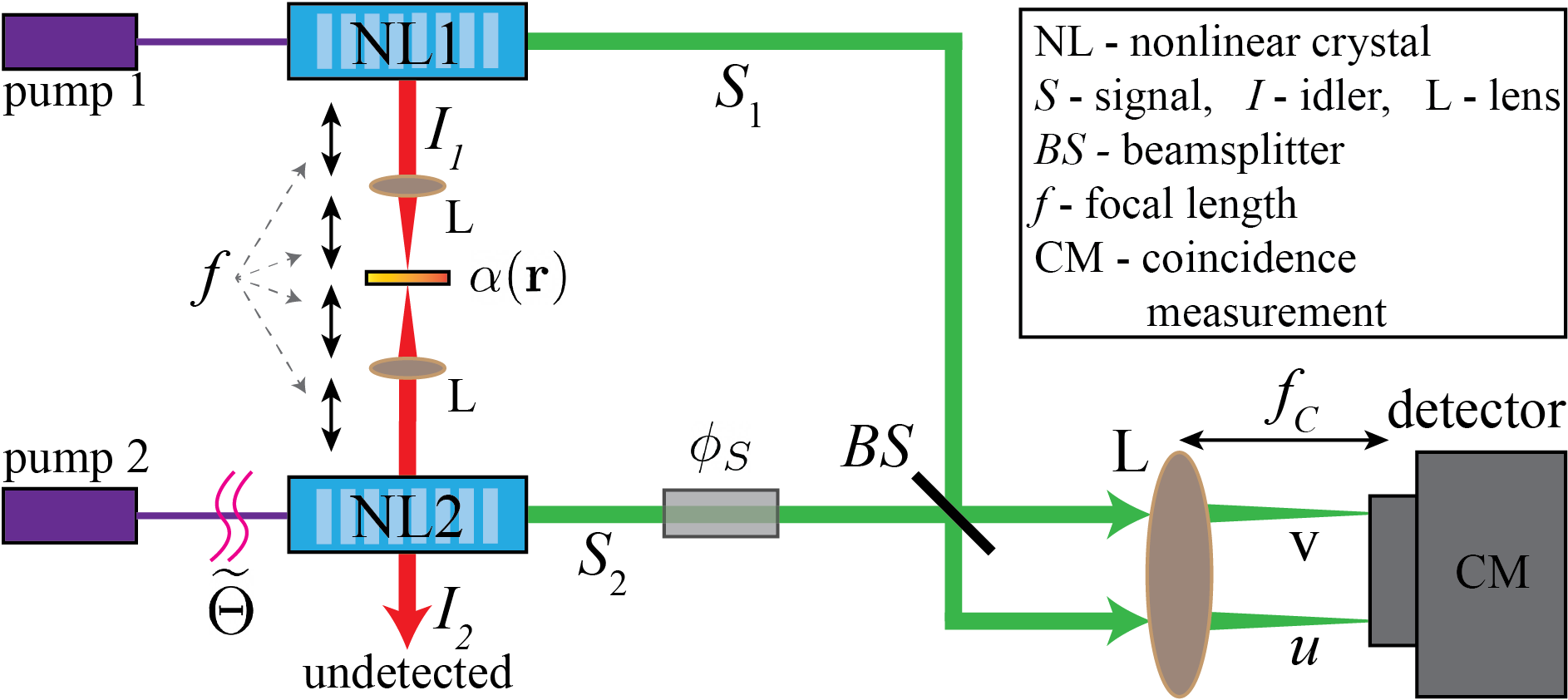
Figure 2: Proposed experimental scheme, also applicable to noise-resistant phase imaging with undetected photons. (For an alternative setup, see SM sup .) Two nonlinear crystals are pumped with mutually incoherent laser beams. Two signal beams are superposed by a beamsplitter (BS) and coincidence counts are measured at two points in an output of BS. Paths of idler photons from the two sources are made identical, resulting in phase-subtractive interference of two signal photons. Information of spatially dependent phase $\alpha(\mathbf{r})$ introduced by a phase object to undetected idler photons appears in the interference pattern.

We consider two nonlinear crystals, NL1 and NL2, which are pumped by two mutually incoherent laser beams of equal intensity (Fig. 2) Her . The incoherent pump beams can in principle originate from independent lasers, or one can introduce a randomly fluctuating phase or long time-delay between two beams originating from the same laser. This situation can be analytically modeled by introducing a random (stochastic) phase difference, $\widetilde{\Theta}$, between the two pump beams, where $\widetilde{\Theta}$ obeys Eq. (2).

Following standard terminology, we call the two photons constituting a pair signal ($S$) and idler ($I$). We first consider the path identity of idler photons, which is essentially sending the idler beam ($I_{1}$) emerging from NL1 through NL2 and perfectly aligning it with the idler beam ($I_{2}$) generated by NL2 (Fig. 2). Note that each beam contains an infinite number of modes (momenta). Without any loss of generality, we choose the far-field configuration used in Ref. Lemos et al. (2014). In this configuration, crystal 1 is imaged onto crystal 2, usually by a 4f lens system (Fig. 2). Let $\phi_{I}$ be the phase change associated with the propagation of the idler field from NL1 to NL2. For well-collimated beams, $\phi_{I}$ is practically independent of the momentum ($\mathbf{k}_{I}$) of an idler photon. Suppose now that a phase object is placed in the idler beam between the two sources in such a way that it is on the Fourier plane of both sources (Fig. 2). Consequently, distinct points on the phase object are impinged by idler photons with distinct momenta. We denote a point on the phase object corresponding to idler-momentum $\mathbf{k}_{I}$ by $\mathbf{r}_{\mathbf{k}_{I}}$. If the phase object introduces a spatially dependent phase ($\alpha$), idler fields at the two sources are related by Lahiri et al. (2015) $\hat{a}_{I_{2}}(\mathbf{k}_{I})=\exp[i\phi_{I}+i\alpha(\mathbf{r}_{\mathbf{k}_{I}})]\hat{a}_{I_{1}}(\mathbf{k}_{I})$, where $\hat{a}$ represents the photon annihilation operator and $\phi_{I}$ does not depend on $\mathbf{k}_{I}$. Combining this relation with the expressions of four-photon states generated by the two SPDC crystals, we find that the quantum state before the beamsplitter is given by (SM sup )

$$|\psi^{(4)}\rangle=\sum_{\begin{subarray}{c}\mathbf{k}_{S},\mathbf{k}_{S}^{\prime}\\ \mathbf{k}_{I},\mathbf{k}_{I}^{\prime}\end{subarray}}|\mathbf{k}_{I},\mathbf{k}_{I}^{\prime}\rangle_{1}\otimes\{C^{(4)}(\mathbf{k}_{S},\mathbf{k}_{S}^{\prime},\mathbf{k}_{I},\mathbf{k}_{I}^{\prime})|\mathbf{k}_{S},\mathbf{k}_{S}^{\prime}\rangle_{1}$$

$$+e^{2i\widetilde{\Theta}}e^{-i[2\phi_{I}+\alpha(\mathbf{r}_{\mathbf{k}_{I}})+\alpha(\mathbf{r}_{\mathbf{k}_{I}^{\prime}})]}C^{(4)}(\mathbf{k}_{S},\mathbf{k}_{S}^{\prime},\mathbf{k}_{I},\mathbf{k}_{I}^{\prime})|\mathbf{k}_{S},\mathbf{k}_{S}^{\prime}\rangle_{2}$$

$$+e^{i\widetilde{\Theta}}e^{-i[\phi_{I}+\alpha(\mathbf{r}_{\mathbf{k}_{I}^{\prime}})]}C^{(2)}(\mathbf{k}_{S},\mathbf{k}_{I})C^{(2)}(\mathbf{k}_{S}^{\prime},\mathbf{k}_{I}^{\prime})|\mathbf{k}_{S}\rangle_{1}|\mathbf{k}_{S}^{\prime}\rangle_{2}\},$$ (6)

where subscripts $1$ and $2$ corresponds to the two crystals, $|\mathbf{k}_{S},\mathbf{k}_{S}^{\prime},\mathbf{k}_{I},\mathbf{k}_{I}^{\prime}\rangle$ denotes a four-photon state in which two signal photons have momenta $\mathbf{k}_{S},\mathbf{k}_{S}^{\prime}$ and two idler photons have momenta $\mathbf{k}_{I},\mathbf{k}_{I}^{\prime}$; $C^{(4)}(\mathbf{k}_{S},\mathbf{k}_{S}^{\prime},\mathbf{k}_{I},\mathbf{k}_{I}^{\prime})=C^{(2)}(\mathbf{k}_{S},\mathbf{k}_{I})C^{(2)}(\mathbf{k}_{S}^{\prime},\mathbf{k}_{I}^{\prime})/2$, and $C^{(2)}$ is proportional to the well-known two-photon probability amplitude generated by SPDC Walborn et al. (2010). Note that two-photon terms do not contribute to the phenomenon in which we are interested and the probability of generation of six or more photon terms is negligible. We observe that Eq. (Phase-Subtractive Interference and Noise-Resistant Quantum Imaging with Two Undetected Photons) is a generalized multi-mode version of Eq. (Phase-Subtractive Interference and Noise-Resistant Quantum Imaging with Two Undetected Photons). The first, second, and third terms inside braces on the right-hand side of Eq. (Phase-Subtractive Interference and Noise-Resistant Quantum Imaging with Two Undetected Photons) represent two signal photons generated, respectively, by NL1, NL2, and both NL1 and NL2.

The two signal beams, $S_{1}$ and $S_{2}$, are superposed by a beamsplitter whose outputs are sent to a detector (e.g., camera) where two-photon coincidence measurements can be performed at various pairs of points (Fig. 2). Since we have chosen the far-field configuration Lemos et al. (2014), the detector is located on the Fourier plane of the two sources (Fig. 2). Therefore, a signal photon with momentum $\mathbf{k}_{S}$ arrives at a point $\mathbf{r}_{\mathbf{k}_{S}}$ on the detector. We assume that both points are located at the same output ($b$). The quantized field at a point $\mathbf{r}_{\mathbf{k}_{S}}$ in output $b$ can be expressed as Lahiri et al. (2015) $\hat{E}^{(+)}_{b}(\mathbf{r}_{\mathbf{k}_{S}})\propto\hat{a}_{{S_{1}}}(\mathbf{k}_{S})+ie^{i\phi_{S}}\hat{a}_{{S_{2}}}(\mathbf{k}_{S})$, where $\phi_{S}$ is phase difference between the two signal beams. For well-collimated beams $\phi_{S}$ is practically independent of $\mathbf{k}_{S}$. The probability of coincidence detection of two signal photons at ($\mathbf{r}_{\mathbf{k}_{S}},\mathbf{r}_{\mathbf{k}_{S}^{\prime}}$) is given by Mandel and Wolf (1995) $P_{bb}^{(2)}(\mathbf{r}_{\mathbf{k}_{S}},\mathbf{r}_{\mathbf{k}_{S}^{\prime}})\propto\langle\psi^{(4)}|\hat{E}^{(-)}_{b}(\mathbf{r}_{\mathbf{k}_{S}})\hat{E}^{(-)}_{b}(\mathbf{r}_{\mathbf{k}_{S}^{\prime}})\hat{E}^{(+)}_{b}(\mathbf{r}_{\mathbf{k}_{S}^{\prime}})\hat{E}^{(+)}_{b}(\mathbf{r}_{\mathbf{k}_{S}})|\psi^{(4)}\rangle$, where $\hat{E}^{(-)}_{b}=\{\hat{E}^{(+)}_{b}\}^{{\dagger}}$. Applying Eqs. (2) and (Phase-Subtractive Interference and Noise-Resistant Quantum Imaging with Two Undetected Photons), we now get the following two-photon phase-subtractive interference pattern:

$$P_{bb}^{(2)}(\mathbf{r}_{\mathbf{k}_{S}},\mathbf{r}_{\mathbf{k}_{S}^{\prime}})$$

$$\propto\sum_{\mathbf{k}_{I},\mathbf{k}_{I}^{\prime}}\big{\{}P^{(4)}_{1}(\mathbf{k}_{S},\mathbf{k}_{S}^{\prime},\mathbf{k}_{I},\mathbf{k}_{I}^{\prime})+P^{(4)}_{2}(\mathbf{k}_{S},\mathbf{k}_{S}^{\prime},\mathbf{k}_{I},\mathbf{k}_{I}^{\prime})$$

$$+P^{(4)}_{12}(\mathbf{k}_{S},\mathbf{k}_{S}^{\prime},\mathbf{k}_{I},\mathbf{k}_{I}^{\prime})[1+\cos\{\alpha(\mathbf{r}_{\mathbf{k}_{I}})-\alpha(\mathbf{r}_{\mathbf{k}_{I}^{\prime}})\}]\big{\}},$$ (7)

where $P^{(4)}_{1}$ and $P^{(4)}_{2}$ are contributions from NL1 and NL2, respectively, while the term containing $P^{(4)}_{12}$ is due to joint emissions at NL1 and NL2 (their explicit forms and cases in which points ($\mathbf{r}_{\mathbf{k}_{S}},\mathbf{r}_{\mathbf{k}_{S}^{\prime}}$) are not located in output $b$ are given in SM sup ).

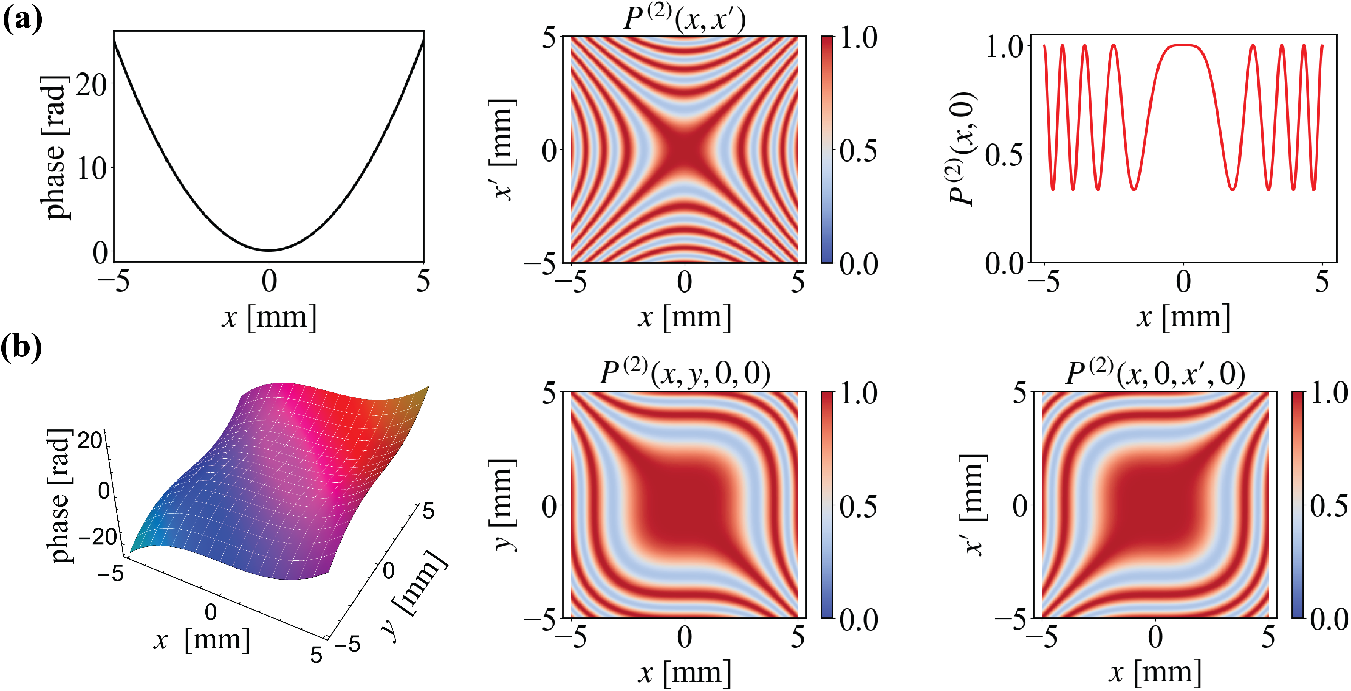
Figure 3: Interferograms containing information of phase objects. Two-photon phase-stable interference patterns are created by detecting signal photons (810 nm) only, but they contain information of spatially dependent phase ($\alpha$) introduced to undetected idler photons (1550 nm). (a) One-dimensional phase $\alpha(x)=x^{2}$ (top left) results in the coincidence counting rate shown in top middle. Coincidence rates along the line $x^{\prime}=0$ on the detector is shown in top right. (b) Two-dimensional phase $\alpha(x,y)=(x^{3}+y^{3})/10$ (bottom left) leads to four-dimensional coincidence map $P^{(2)}(x,y;x^{\prime},y^{\prime})$. The $xy$-plane cross-section (bottom middle) and $xx^{\prime}$-plane cross-section (bottom right) of the coincidence map are shown.

Imaging: It is evident from Eq. (Phase-Subtractive Interference and Noise-Resistant Quantum Imaging with Two Undetected Photons) that the interferogram depends on the spatially dependent phase ($\alpha$) introduced by the object to undetected idler photons. For the purpose of illustration, let us consider a case in which the signal (810 nm) and idler (1550 nm) photons are maximally correlated in momenta sup . We consider two phase objects represented by (a) a one-dimensional (1D) quadratic phase profile $\alpha(x)=x^{2}$ and (b) a two-dimensional (2D) cubic phase profile $\alpha(x,y)=(x^{3}+y^{3})/10$. For the 1D phase object, the coincidence counting rate depends on two coordinates $(x,x^{\prime})$, i.e., $P^{(2)}(\mathbf{r}_{\mathbf{k}_{S}},\mathbf{r}_{\mathbf{k}_{S}^{\prime}})\equiv P^{(2)}(x,x^{\prime})$. Figure 3a illustrates the corresponding two-photon interference pattern. For a 2D phase object, the coincidence map depends on four coordinates $(x,y,x^{\prime},y^{\prime})$, i.e., $P^{(2)}(\mathbf{r}_{\mathbf{k}_{S}},\mathbf{r}_{\mathbf{k}_{S}^{\prime}})\equiv P^{(2)}(x,y,x^{\prime},y^{\prime})$. Figure 3b shows two cross-sections of the coincidence map: $xy$-plane (middle) and $xx^{\prime}$-plane (right), each displaying interference patterns.

One can readily reconstruct the phase profile of an object from such interference patterns (coincidence maps). Methods of reconstructing phase profiles from coincidence maps have been demonstrated in Refs. Szuniewicz et al. (2023); Thekkadath et al. (2023). Such methods employ standard phase-unwrapping algorithms Herráez et al. (2002); Mertz (2019) and can be immediately applied to interferograms generated by our proposed scheme. Therefore, like standard quantum imaging with undetected photons (QIUP), our method is applicable to retrieve phase image at a wavelength for which adequate detectors are not available. However, standard QUIP becomes inapplicable when random phase fluctuations (noise) destroy the single-photon interference patterns. Our method works even in such a scenario as we discuss below.

Phase Stability: Equation (Phase-Subtractive Interference and Noise-Resistant Quantum Imaging with Two Undetected Photons) is a multi-mode version of Eq. (5). Note that outputs $g$ and $h$ in Fig. 1b are both located at output $b$ in Fig. 2 and correspond to points $\mathbf{r}_{\mathbf{k}_{S}}$ and $\mathbf{r}_{\mathbf{k}_{S}^{\prime}}$. The phases gained by two signal photons detected at $\mathbf{r}_{\mathbf{k}_{S}}$ and $\mathbf{r}_{\mathbf{k}_{S}^{\prime}}$ get added with opposite signs. Since $\phi_{S}$ (Fig. 2) is spatially independent, these two phases cancel each other. Likewise, the spatially independent phase ($\phi_{I}$) gained by undetected idler photons does not appear in the interference pattern. Furthermore, the phase difference between the pump beams is irrelevant because these beams are mutually incoherent. Since spatially independent phases due to propagation of pump, signal, and idler photons make up the tunable interferometric phase, the interference pattern [Eq. (Phase-Subtractive Interference and Noise-Resistant Quantum Imaging with Two Undetected Photons)] is independent of the tunable interferometric phase. Standard QIUP experiments heavily rely on the stability of this interferometric phase, which is subject to random fluctuations due to instability of the interferometer. In our case, the two-photon interferograms do not depend on the interferometric phase and, consequently, are immune to any such fluctuations. Our imaging scheme also works when the sources are not independent but the single-photon interference is destroyed by high phase noise in signal or idler arms. Finally, we stress that no single-photon interference can occur in our scheme.

In summary, we have presented a theory of two-particle interferometry that employs four-particle states generated by two independent sources and is enabled by path identity of two undetected particles. The interference patterns are independent of the tunable interferometric phase and contain information of spatially dependent phases acquired by undetected particles. An application of this phenomenon is a quantum imaging technique that, like standard QIUP, can acquire images at wavelengths for which no detectors are available. However, our technique applies when standard QIUP fails due to the presence of high phase-noise. Our technique also allows one to have arbitrarily long photon acquisition time, which is especially useful for imaging with low-intensity light. The principle of standard QIUP has been applied to reconstruct object information in various fields, e.g., spectroscopy Kalashnikov et al. (2016), microscopy Kviatkovsky et al. (2020); Paterova et al. (2020), holography Töpfer et al. (2022) and optical coherence tomography Vallés et al. (2018); Paterova et al. (2018). Our results are applicable to all these fields.

Acknowledgment: The research was supported by the U.S. Office of Naval Research under award number N00014-23-1-2778.

Supplementary material

I An analysis of standard two-photon interference

In this section, we derive Eq. (1) of the main text.

The basic features of a standard two-particle interference are illustrated by Fig. 1a (top) in the main text. There are two sources, $Q_{1}$ and $Q_{2}$, each of which can emit a pair of identical particles. $Q_{1}$ can emit the particle pair into beams $u$ and $v$, and $Q_{2}$ can emit the pair into beams $c$ and $d$. When the sources emit coherently and with equal probability, the two-particle state generated by them is given by Horne et al. (1989)

$$|\psi\rangle=\frac{1}{\sqrt{2}}(|S_{u}\rangle_{1}|S_{v}\rangle_{1}+|S_{c}\rangle_{2}|S_{d}\rangle_{2}),$$ (S1)

where $|S_{u}\rangle_{1}$ denotes a single particle $S$ that is emitted from $Q_{1}$ and in beam $u$, etc. State $|S_{u}\rangle_{1}$ can be expressed as

$$|S_{u}\rangle_{1}=\hat{a}^{\dagger}_{1}(u)|\text{vac}\rangle,$$ (S2)

where $|\text{vac}\rangle$ represents the vacuum state, $\hat{a}_{1}^{\dagger}(u)$ is the creation operator for particle $S$ created from source $Q_{1}$ in path $u$. Note that particle $S$ can be a boson or a fermion. Likewise, we can write $|S_{v}\rangle_{1}=\hat{a}^{\dagger}_{1}(v)|\text{vac}\rangle$, $|S_{c}\rangle_{2}=\hat{a}^{\dagger}_{2}(c)|\text{vac}\rangle$, and $|S_{d}\rangle_{2}=\hat{a}^{\dagger}_{2}(d)|\text{vac}\rangle$.

Beams $u$ and $c$ are combined by a beamsplitter with outputs $h$ and $h^{\prime}$. The tunable phase difference between beams $u$ and $c$ is denoted by $\phi_{S}$. Likewise, beams $v$ and $d$ are superposed with phase difference $\phi_{S}^{\prime}$ by another beamsplitter with outputs $g$ and $g^{\prime}$. Detectors are placed at outputs $h$ and $g$. The field operators at these detectors are given by standard expressions

$$\hat{a}_{S}(h)=\frac{1}{\sqrt{2}}[\hat{a}_{1}(u)+ie^{i\phi_{S}}\hat{a}_{2}(c)],$$ (S3a)

$$\hat{a}_{S}(g)=\frac{1}{\sqrt{2}}[\hat{a}_{1}(v)+ie^{i\phi_{S}^{\prime}}\hat{a}_{2}(d)].$$ (S3b)

The probability of joint detection of two $S$-particles at $g$ and $h$ is given by $P_{hg}\equiv\langle\psi|\hat{a}^{\dagger}_{S}(h)\hat{a}^{\dagger}_{S}(g)\hat{a}_{S}(g)\hat{a}_{S}(h)|\psi\rangle$. Using Eqs. (S1), (S3a), and (S3b), we readily obtain Eq. (1) of the main text:

$$P_{hg}\propto 1-\cos(\phi_{S}+\phi_{S}^{\prime}),$$ (S4)

which represents a typical two-particle interference pattern.

II Recollection of the basic results from the theory of SPDC

In this section, we recollect relevant results form the theory of spontaneous parametric down-conversion (SPDC) in a nonlinear crystal. The scalar treatment is enough for our purpose.

In the interaction picture, the Hamiltonian of the SPDC process can be written as Walborn et al. (2010)

$$\hat{H}_{\text{in}}(t) =\int_{D}d^{3}r~{}\tilde{\chi}E_{P}(\mathbf{r},t)\hat{E}^{(-)}_{S}(\mathbf{r},t)\hat{E}^{(-)}_{I}(\mathbf{r},t)+\text{H.c.},$$ (S5)

where $\tilde{\chi}$ is the nonlinear electric susceptibility of the crystal, $\hat{E}^{(-)}_{S}$ ($\hat{E}^{(-)}_{I}$) is the negative frequency part of the electric field operator corresponding to the signal (idler) photon, and H.c. represents Hermitian conjugate. The complex quantity $E_{P}$ represents the classical pump field, and $D$ is the volume of the crystal.

A well-collimated and narrow-band pump field can be represented by a classical monochromatic plane wave,

$$E_{P}(\mathbf{r},t)=V_{P}\exp[i(\mathbf{k}_{P}\cdot\mathbf{r}-\omega_{P}t)],$$ (S6)

where $V_{P}$ is the complex amplitude of the pump wave, $\mathbf{k}_{P}$ is the associated wave vector, and $\omega_{P}$ is the angular frequency. Quantum fields associated with signal and idler photons are represented by their plane wave mode decomposition Walborn et al. (2010)

$$\hat{E}^{(+)}_{S}(\mathbf{r},t)=\sum_{\mathbf{k}_{S}}\beta(\omega_{S})\exp[i(\mathbf{k}_{S}\cdot\mathbf{r}-\omega_{S}t)]\hat{a}_{S}(\mathbf{k}_{S}),$$ (S7a)

$$\hat{E}^{(+)}_{I}(\mathbf{r},t)=\sum_{\mathbf{k}_{I}}\beta(\omega_{I})\exp[i(\mathbf{k}_{I}\cdot\mathbf{r}-\omega_{I}t)]\hat{a}_{I}(\mathbf{k}_{I}).$$ (S7b)

Here, $\hbar\mathbf{k}$ and $\omega=c|\mathbf{k}|$ represent the momentum and angular frequency corresponding to each plane wave mode, respectively, $\hat{E}^{(+)}\equiv\{\hat{E}^{(-)}\}^{\dagger}$, $\beta(\omega)=i\sqrt{\hbar\omega/(2\epsilon_{0}n^{2}L^{3})}$, $\epsilon_{0}$ is the electric permittivity of free space, $n$ is the refractive index of the crystal, $L^{3}$ is the quantization volume, and $\hat{a}(\mathbf{k})$ is the photon annihilation operator for a photon in mode labeled by $\mathbf{k}$.

Substituting from Eqs. (S7a) and (S7b) into Eq. (S5), one finds that

$$\hat{H}_{\text{in}}(t) =\sum_{\mathbf{k}_{S},\mathbf{k}_{I}}\tilde{\chi}(\omega_{S},\omega_{I})V_{P}\beta^{*}(\omega_{S})\beta^{*}(\omega_{I})$$

$$\times\exp[i(\omega_{S}+\omega_{I}-\omega_{P})t]\hat{a}^{{\dagger}}_{S}(\mathbf{k}_{S})\hat{a}^{{\dagger}}_{I}(\mathbf{k}_{I})$$

$$\times\int_{V}d^{3}r~{}\exp[i(\mathbf{k}_{P}-\mathbf{k}_{S}-\mathbf{k}_{I})\cdot\mathbf{r})]+\text{H.c.}$$ (S8)

The quantum state of the light generated by down conversion at the crystal is then given by

$$|\psi(t)\rangle=\hat{U}(t)|\text{vac}\rangle,$$ (S9)

where $|\text{vac}\rangle$ is the vacuum state and $\hat{U}(t)$ is given by the standard perturbative expression (see, for example, Ref. Cohen-Tannoudji et al. (1977))

$$\hat{U}(t)=\hat{\openone}+\frac{1}{i\hbar}\int_{0}^{t}d\tau\hat{H}_{\text{in}}(\tau)$$

$$+\left(\frac{1}{i\hbar}\right)^{2}\int_{0}^{t}d\tau\int_{0}^{\tau}d\tau^{\prime}\hat{H}_{\text{in}}(\tau)\hat{H}_{\text{in}}(\tau^{\prime})+\cdots.$$ (S10)

Evaluating the integrals allows the state to be expressed in the form

$$|\psi\rangle \propto|\text{vac}\rangle+\sum_{\mathbf{k}_{S},\mathbf{k}_{I}}C^{(2)}(\mathbf{k}_{S},\mathbf{k}_{I})|\mathbf{k}_{S},\mathbf{k}_{I}\rangle$$

$$+\sum_{\begin{subarray}{c}\mathbf{k}_{S},\mathbf{k}_{S}^{\prime}\\ \mathbf{k}_{I},\mathbf{k}_{I}^{\prime}\end{subarray}}C^{(4)}(\mathbf{k}_{S},\mathbf{k}_{S}^{\prime},\mathbf{k}_{I},\mathbf{k}_{I}^{\prime})|\mathbf{k}_{S},\mathbf{k}_{S}^{\prime},\mathbf{k}_{I},\mathbf{k}_{I}^{\prime}\rangle+\cdots,$$ (S11)

where

$$C^{(2)}(\mathbf{k}_{S},\mathbf{k}_{I})=\frac{Dt}{i\hbar}V_{P}\tilde{\chi}(\omega_{S},\omega_{I})\beta^{*}(\omega_{S})\beta^{*}(\omega_{I})$$

$$\qquad\qquad\times\exp[i\Delta\omega t/2]\exp[-i\Delta\mathbf{k}\cdot\mathbf{r}_{0}]$$

$$\qquad\qquad\times\operatorname{sinc}(\Delta\omega t/2)\prod_{m=1}^{3}\operatorname{sinc}(\Delta k_{m}\ell_{m}/2),$$ (S12a)

$$C^{(4)}(\mathbf{k}_{S},\mathbf{k}_{S}^{\prime},\mathbf{k}_{I},\mathbf{k}_{I}^{\prime})=\frac{1}{2}C^{(2)}(\mathbf{k}_{S},\mathbf{k}_{I})C^{(2)}(\mathbf{k}_{S}^{\prime},\mathbf{k}_{I}^{\prime}).$$ (S12b)

In Eqs. (S12a) and (S12b), $\Delta\omega\equiv\omega_{S}+\omega_{I}-\omega_{P}$, $\Delta\mathbf{k}\equiv\mathbf{k}_{S}+\mathbf{k}_{I}-\mathbf{k}_{P}$, and $\mathbf{r}_{0}$ represents the position of the center of the crystal with side lengths of $\ell_{1}$, $\ell_{2}$, and $\ell_{3}$. Note that $C^{(2)}$ can be modeled by well-behaved functions which agree very well with experimental observations Walborn et al. (2010).

III Derivation of Eq. (6) in Main Text

In this section, we show how to determine the four-photon quantum state (Eq. (6) in the main text) before the beamsplitter in the setup illustrated by Fig. 2 in the main text.

Since the two nonlinear crystals are pumped by mutually incoherent pump beams of equal intensity, the two pump fields $E_{P_{1}}$ and $E_{P_{2}}$ are related by $E_{P_{2}}=e^{i\widetilde{\Theta}}E_{P_{1}}$. Here, $\widetilde{\Theta}$ is a random (stochastic) phase obeying Eq. (2) of main text, i.e., $\langle e^{i(\widetilde{\Theta}+\phi)}\rangle=\langle\sin(\widetilde{\Theta}+\phi)\rangle=\langle\cos(\widetilde{\Theta}+\phi)\rangle=0,$ where $\phi$ represents an arbitrary phase.

When two nonlinear crystals, NL1 and NL2, are pumped simultaneously, the resulting state can be expressed as Liu et al. (2009); Lahiri et al. (2019) $|\tilde{\psi}\rangle=\hat{U}_{2}\hat{U}_{1}|\text{vac}\rangle$, where $j$ corresponds to crystal NL$j$ and $\hat{U}$ is defined by Eq. (II). We assume that the intensity of each pump beam is $|V_{P}|^{2}$.

We note that two-photon terms do not contribute to the phenomenon we are interested: they yield zero coincidence counts in our case. Furthermore, the probability of generation of six or more photon terms is negligible compared to that of four-photon terms. Therefore, we only consider four-photon terms generated by the system. It follows from Eqs. (II), (II), and the expression $|\tilde{\psi}\rangle=\hat{U}_{2}\hat{U}_{1}|\text{vac}\rangle$ that the four-photon terms generated by the two sources have the form

$$| \tilde{\psi}^{(4)}\rangle=\sum_{\begin{subarray}{c}\mathbf{k}_{S},\mathbf{k}_{S}^{\prime}\\ \mathbf{k}_{I},\mathbf{k}_{I}^{\prime}\end{subarray}}C^{(4)}(\mathbf{k}_{S},\mathbf{k}_{S}^{\prime},\mathbf{k}_{I},\mathbf{k}_{I}^{\prime})|\mathbf{k}_{S},\mathbf{k}_{S}^{\prime},\mathbf{k}_{I},\mathbf{k}_{I}^{\prime}\rangle_{1}$$

$$+e^{i2\widetilde{\Theta}}\sum_{\begin{subarray}{c}\mathbf{k}_{S},\mathbf{k}_{S}^{\prime}\\ \mathbf{k}_{I},\mathbf{k}_{I}^{\prime}\end{subarray}}C^{(4)}(\mathbf{k}_{S},\mathbf{k}_{S}^{\prime},\mathbf{k}_{I},\mathbf{k}_{I}^{\prime})|\mathbf{k}_{S},\mathbf{k}_{S}^{\prime},\mathbf{k}_{I},\mathbf{k}_{I}^{\prime}\rangle_{2}$$

$$+e^{i\widetilde{\Theta}}\Big{[}\sum_{\mathbf{k}_{S},\mathbf{k}_{I}}C^{(2)}(\mathbf{k}_{S},\mathbf{k}_{I})|\mathbf{k}_{S},\mathbf{k}_{I}\rangle_{1}\Big{]}$$

$$\qquad\otimes\Big{[}\sum_{\mathbf{k}_{S}^{\prime},\mathbf{k}_{I}^{\prime}}C^{(2)}(\mathbf{k}_{S}^{\prime},\mathbf{k}_{I}^{\prime})|\mathbf{k}_{S}^{\prime},\mathbf{k}_{I}^{\prime}\rangle_{2}\Big{]},$$ (S13)

where subscripts $1$ and $2$ represent the two crystals, $|\mathbf{k}_{S},\mathbf{k}_{S}^{\prime},\mathbf{k}_{I},\mathbf{k}_{I}^{\prime}\rangle$ denotes a four-photon state in which two signal photons have momenta $\mathbf{k}_{S},\mathbf{k}_{S}^{\prime}$ and two idler photons have momenta $\mathbf{k}_{I},\mathbf{k}_{I}^{\prime}$; quantities $C^{(2)}$ and $C^{(4)}$ are given by Eqs. (S12a) and (S12b), respectively. Note that $C^{(2)}$ can be modeled by well-behaved functions which agree very well with experimental observations Walborn et al. (2010).

As mentioned in the main text, path identity of idler photons and the effect of the phase object can be represented by the relation $\hat{a}_{I_{2}}(\mathbf{k}_{I})=\exp[i\phi_{I}+i\alpha(\mathbf{r}_{\mathbf{k}_{I}})]\hat{a}_{I_{1}}(\mathbf{k}_{I})$. Using the relation $|\mathbf{k}_{I}\rangle_{j}=\hat{a}_{I_{j}}^{{\dagger}}(\mathbf{k}_{I})|0\rangle$, we readily find that

$$|\mathbf{k}_{I}\rangle_{2}=\exp[-i\alpha(\mathbf{r}_{\mathbf{k}_{I}})-i\phi_{I}]|\mathbf{k}_{I}\rangle_{1}.$$ (S14)

Now, substituting from Eq. (S14) into Eq. (III), we obtain Eq. (6) of the main text:

$$|\psi^{(4)}\rangle=\sum_{\begin{subarray}{c}\mathbf{k}_{S},\mathbf{k}_{S}^{\prime}\\ \mathbf{k}_{I},\mathbf{k}_{I}^{\prime}\end{subarray}}|\mathbf{k}_{I},\mathbf{k}_{I}^{\prime}\rangle_{1}\otimes\Big{\{}C^{(4)}(\mathbf{k}_{S},\mathbf{k}_{S}^{\prime},\mathbf{k}_{I},\mathbf{k}_{I}^{\prime})|\mathbf{k}_{S},\mathbf{k}_{S}^{\prime}\rangle_{1}$$

$$+e^{2i\widetilde{\Theta}}e^{-i[2\phi_{I}+\alpha(\mathbf{r}_{\mathbf{k}_{I}})+\alpha(\mathbf{r}_{\mathbf{k}_{I}^{\prime}})]}C^{(4)}(\mathbf{k}_{S},\mathbf{k}_{S}^{\prime},\mathbf{k}_{I},\mathbf{k}_{I}^{\prime})|\mathbf{k}_{S},\mathbf{k}_{S}^{\prime}\rangle_{2}$$

$$+e^{i\widetilde{\Theta}}e^{-i[\phi_{I}+\alpha(\mathbf{r}_{\mathbf{k}_{I}^{\prime}})]}C^{(2)}(\mathbf{k}_{S},\mathbf{k}_{I})C^{(2)}(\mathbf{k}_{S}^{\prime},\mathbf{k}_{I}^{\prime})|\mathbf{k}_{S}\rangle_{1}|\mathbf{k}_{S}^{\prime}\rangle_{2}\Big{\}}.$$ (S15)

IV Explicit forms of $P^{(4)}_{1}$, $P^{(4)}_{2}$, and $P^{(4)}_{12}$ in Eq. (7) of main text

In this section, we provide expressions for $P^{(4)}_{1}$, $P^{(4)}_{2}$, and $P^{(4)}_{12}$, which appear in the formula of $P_{bb}^{(2)}(\mathbf{r}_{\mathbf{k}_{S}},\mathbf{r}_{\mathbf{k}_{S}^{\prime}})$ given by Eq. (7) of the main text.

The three terms on the right-hand side of Eq. (6) in main text [Eq. (III)] arise, respectively, due to emission from NL1 only, emission from NL2 only, and joint emissions from NL1 and NL2. Let us represent these three terms by $|\psi_{1}^{(4)}\rangle$, $|\psi_{2}^{(4)}\rangle$, and $|\psi_{12}^{(4)}\rangle$, respectively. That is, $|\psi^{(4)}\rangle=|\psi_{1}^{(4)}\rangle+|\psi_{1}^{(4)}\rangle+|\psi_{12}^{(4)}\rangle$. It is given in the main text that $P_{bb}^{(2)}(\mathbf{r}_{\mathbf{k}_{S}},\mathbf{r}_{\mathbf{k}_{S}^{\prime}})\propto\langle\psi^{(4)}|\hat{E}^{(-)}_{b}(\mathbf{r}_{\mathbf{k}_{S}})\hat{E}^{(-)}_{b}(\mathbf{r}_{\mathbf{k}_{S}^{\prime}})\hat{E}^{(+)}_{b}(\mathbf{r}_{\mathbf{k}_{S}^{\prime}})\hat{E}^{(+)}_{b}(\mathbf{r}_{\mathbf{k}_{S}})|\psi^{(4)}\rangle$. Using this formula, we readily find that

$$P_{1}^{(4)}(\mathbf{k}_{S},\mathbf{k}_{S}^{\prime},\mathbf{k}_{I},\mathbf{k}_{I}^{\prime})$$

$$\propto\langle\psi_{1}^{(4)}|\hat{E}^{(-)}_{b}(\mathbf{r}_{\mathbf{k}_{S}})\hat{E}^{(-)}_{b}(\mathbf{r}_{\mathbf{k}_{S}^{\prime}})\hat{E}^{(+)}_{b}(\mathbf{r}_{\mathbf{k}_{S}^{\prime}})\hat{E}^{(+)}_{b}(\mathbf{r}_{\mathbf{k}_{S}})|\psi_{1}^{(4)}\rangle$$

$$=\big{|}C^{(4)}(\mathbf{k}_{S},\mathbf{k}_{S}^{\prime},\mathbf{k}_{I},\mathbf{k}_{I}^{\prime})+C^{(4)}(\mathbf{k}_{S},\mathbf{k}_{S}^{\prime},\mathbf{k}_{I}^{\prime},\mathbf{k}_{I})$$

$$+C^{(4)}(\mathbf{k}_{S}^{\prime},\mathbf{k}_{S},\mathbf{k}_{I},\mathbf{k}_{I}^{\prime})+C^{(4)}(\mathbf{k}_{S}^{\prime},\mathbf{k}_{S},\mathbf{k}_{I}^{\prime},\mathbf{k}_{I})\big{|}^{2},$$ (S16a)

$$P_{2}^{(4)}(\mathbf{k}_{S},\mathbf{k}_{S}^{\prime},\mathbf{k}_{I},\mathbf{k}_{I}^{\prime})$$

$$\propto\langle\psi_{2}^{(4)}|\hat{E}^{(-)}_{b}(\mathbf{r}_{\mathbf{k}_{S}})\hat{E}^{(-)}_{b}(\mathbf{r}_{\mathbf{k}_{S}^{\prime}})\hat{E}^{(+)}_{b}(\mathbf{r}_{\mathbf{k}_{S}^{\prime}})\hat{E}^{(+)}_{b}(\mathbf{r}_{\mathbf{k}_{S}})|\psi_{2}^{(4)}\rangle$$

$$=\big{|}C^{(4)}(\mathbf{k}_{S},\mathbf{k}_{S}^{\prime},\mathbf{k}_{I},\mathbf{k}_{I}^{\prime})+C^{(4)}(\mathbf{k}_{S},\mathbf{k}_{S}^{\prime},\mathbf{k}_{I}^{\prime},\mathbf{k}_{I})$$

$$+C^{(4)}(\mathbf{k}_{S}^{\prime},\mathbf{k}_{S},\mathbf{k}_{I},\mathbf{k}_{I}^{\prime})+C^{(4)}(\mathbf{k}_{S}^{\prime},\mathbf{k}_{S},\mathbf{k}_{I}^{\prime},\mathbf{k}_{I})\big{|}^{2},$$ (S16b)

$$P_{12}^{(4)}(\mathbf{k}_{S},\mathbf{k}_{S}^{\prime},\mathbf{k}_{I},\mathbf{k}_{I}^{\prime})$$

$$\propto\langle\psi_{12}^{(4)}|\hat{E}^{(-)}_{b}(\mathbf{r}_{\mathbf{k}_{S}})\hat{E}^{(-)}_{b}(\mathbf{r}_{\mathbf{k}_{S}^{\prime}})\hat{E}^{(+)}_{b}(\mathbf{r}_{\mathbf{k}_{S}^{\prime}})\hat{E}^{(+)}_{b}(\mathbf{r}_{\mathbf{k}_{S}})|\psi_{12}^{(4)}\rangle$$

$$=\big{|}C^{(2)}(\mathbf{k}_{S},\mathbf{k}_{I})C^{(2)}(\mathbf{k}_{S}^{\prime},\mathbf{k}_{I}^{\prime})$$

$$\qquad+C^{(2)}(\mathbf{k}_{S},\mathbf{k}_{I}^{\prime})C^{(2)}(\mathbf{k}_{S}^{\prime},\mathbf{k}_{I})\big{|}^{2}.$$ (S16c)

V Coincidence counts when both detection points are not located at beamsplitter-output $b$

In the main text, we considered the case in which coincidence counts were measured at a single output ($b$) of the beamsplitter (Fig. 2). Here we provide forms of the coincidence counting rate (joint probability of detecting two photons) in the following cases: (i) both points are located in output $b^{\prime}$, and (ii) one point is located at $b$ and the other at $b^{\prime}$. The method of determining these coincidence counting rates is strictly similar to that presented in the main text.

A general expression for the coincidence counting rate at a pair of points $(\mathbf{r}_{\mathbf{k}_{S}},\mathbf{r}_{\mathbf{k}_{S}^{\prime}})$ is given by

$$P_{jl}^{(2)}(\mathbf{r}_{\mathbf{k}_{S}},\mathbf{r}_{\mathbf{k}_{S}^{\prime}})=\big{\|}\hat{E}^{(+)}_{j}(\mathbf{r}_{\mathbf{k}_{S}^{\prime}})\hat{E}^{(+)}_{l}(\mathbf{r}_{\mathbf{k}_{S}})|\psi^{(4)}\rangle\big{\|}^{2},$$ (S17)

where $j=b,b^{\prime}$ and $l=b,b^{\prime}$ represent outputs of the beamsplitter, $\hat{E}^{(+)}_{j}(\mathbf{r}_{\mathbf{k}_{S}^{\prime}})$ represents the positive frequency part of the quantized electric field at output $j$, and $|\psi^{(4)}\rangle$ is given by Eq. (III) [Eq. (6) of the main text]. We note that $P_{jl}^{(2)}(\mathbf{r}_{\mathbf{k}_{S}},\mathbf{r}_{\mathbf{k}_{S}^{\prime}})=P_{lj}^{(2)}(\mathbf{r}_{\mathbf{k}_{S}},\mathbf{r}_{\mathbf{k}_{S}^{\prime}})$

We first consider the case in which both points are located at the output $b^{\prime}$. In this case, we have $\hat{E}^{(+)}_{b^{\prime}}(\mathbf{r}_{\mathbf{k}_{S}})\propto i\hat{a}_{S_{1}}(\mathbf{k}_{S})+e^{i\phi_{S}}\hat{a}_{S_{2}}(\mathbf{k}_{S}^{\prime})$. From Eqs. (III) and (S17), it follows that

$$P^{(2)}_{b^{\prime}b^{\prime}}(\mathbf{r}_{\mathbf{k}_{S}},\mathbf{r}_{\mathbf{k}_{S}^{\prime}})\propto\sum_{\mathbf{k}_{I},\mathbf{k}_{I}^{\prime}}P_{1}^{(4)}(\mathbf{k}_{S},\mathbf{k}_{S}^{\prime},\mathbf{k}_{I},\mathbf{k}_{I}^{\prime})$$

$$+P_{2}^{(4)}(\mathbf{k}_{S},\mathbf{k}_{S}^{\prime},\mathbf{k}_{I},\mathbf{k}_{I}^{\prime})$$

$$+P^{(4)}_{12}(\mathbf{k}_{S},\mathbf{k}_{S}^{\prime},\mathbf{k}_{I},\mathbf{k}_{I}^{\prime})\big{\{}1+\cos[\alpha(\mathbf{r}_{\mathbf{k}_{I}})-\alpha(\mathbf{r}_{\mathbf{k}_{I}^{\prime}})]\big{\}}.$$ (S18)

It is to be noted that $P^{(2)}_{b^{\prime}b^{\prime}}$ has the same expression as $P^{(2)}_{bb}$.

We now determine the coincidence counting rate for the case in which one point is located at $b$ and the other at $b^{\prime}$. Using expressions of $\hat{E}^{(+)}_{b}$ (given in main text) and $\hat{E}^{(+)}_{b^{\prime}}$ (given above by Eq. V), we find from Eqs. (III) and (S17) that

$$P^{(2)}_{bb^{\prime}}(\mathbf{r}_{\mathbf{k}_{S}},\mathbf{r}_{\mathbf{k}_{S}^{\prime}})=P^{(2)}_{b^{\prime}b}(\mathbf{r}_{\mathbf{k}_{S}},\mathbf{r}_{\mathbf{k}_{S}^{\prime}})$$

$$\propto \sum_{\mathbf{k}_{I},\mathbf{k}_{I}^{\prime}}P_{1}^{(4)}(\mathbf{k}_{S},\mathbf{k}_{S}^{\prime},\mathbf{k}_{I},\mathbf{k}_{I}^{\prime})+P_{2}^{(4)}(\mathbf{k}_{S},\mathbf{k}_{S}^{\prime},\mathbf{k}_{I},\mathbf{k}_{I}^{\prime})$$

$$+\widetilde{P}^{(4)}_{12}(\mathbf{k}_{S},\mathbf{k}_{S}^{\prime},\mathbf{k}_{I},\mathbf{k}_{I}^{\prime})\big{\{}1-\cos[\alpha(\mathbf{r}_{\mathbf{k}_{I}})-\alpha(\mathbf{r}_{\mathbf{k}_{I}^{\prime}})]\big{\}},$$ (S19)

where

$$\widetilde{P}^{(4)}_{12}(\mathbf{k}_{S},\mathbf{k}_{S}^{\prime},\mathbf{k}_{I},\mathbf{k}_{I}^{\prime})=\big{|} C^{(2)}(\mathbf{k}_{S},\mathbf{k}_{I})C^{(2)}(\mathbf{k}_{S}^{\prime},\mathbf{k}_{I}^{\prime})$$

$$-C^{(2)}(\mathbf{k}_{S},\mathbf{k}_{I}^{\prime})C^{(2)}(\mathbf{k}_{S}^{\prime},\mathbf{k}_{I})\big{|}^{2}.$$ (S20)

VI The special case of perfect momentum correlation between signal and idler photons

In this section, we briefly discuss the scenario considered to produce Fig. 3 in the main text. In this scenario, we assumed signal and idler photons are fully correlated in momenta.

In our case, the two identical crystals are illuminated by pump beams of equal intensity. Using Eqs. (S12b) and (S16a)–(S16c), we find that in our case

$$P^{(4)}_{1}=P^{(4)}_{2}=P^{(4)}_{12}\equiv P_{0}^{(4)}.$$ (S21)

When signal and idler photons are perfectly correlated (delta correlated), Eq. (7) in the main text reduces to

$$P^{(2)}_{bb}(x,y;x^{\prime},y^{\prime})\propto 1+\frac{1}{2}\cos[\alpha(x,y)-\alpha(x^{\prime},y^{\prime})],$$ (S22)

where we have assumed the magnification of the system is unity (i.e., $\mathbf{r}_{\mathbf{k}_{S}}=\mathbf{r}_{\mathbf{k}_{I}}$) and have written $\mathbf{r}_{\mathbf{k}_{S}}\equiv(x,y)$ and $\mathbf{r}_{\mathbf{k}_{S}^{\prime}}\equiv(x^{\prime},y^{\prime})$.

VII An alternative setup to realize phase-subtractive two-photon interference by path identity and noise-resistant quantum phase imaging with undetected photons

In this section, we present an alternative setup (Fig. 4) that can be used to experimentally realize phase-subtractive interference by path identity and noise-resistant phase imaging with undetected photons. The setup is inspired by an experiment performed by Herzog et al. Herzog et al. (1994).

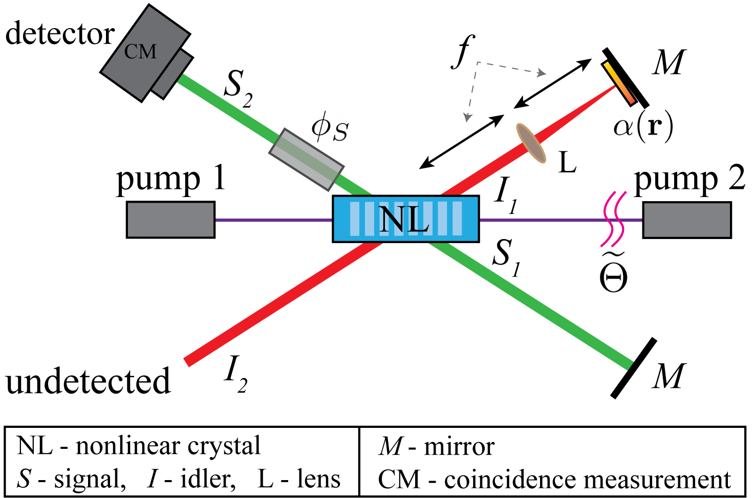
Figure 4: An alternative setup that employs a single crystal. The crystal is pumped from two sides by two mutually-incoherent pump beams with stochastic phase difference $\widetilde{\Theta}$. Mirrors are used to align paths of signal and idler photons by reflecting them back through the crystals. Signal photons are then detected, while idler photons are not.

In contrast to the setup presented by Fig. 2 in the main text, this setup (Fig. 4) employs only one nonlinear crystal. Furthermore, the geometry of the setup discussed in the main text is similar to that of a Mach-Zehnder interferometer, whereas the geometry of the setup presented here is more similar to that of a Michelson interferometer. Despite these differences, these two setups work under the same principle.

As shown in Fig. 4, a nonlinear crystal is pumped from two sides by two mutually incoherent pump beams. We call these two pump beams pump 1 and pump 2. Signal and idler photons generated by SPDC due to pump 1 propagate in beams $S_{1}$ and $I_{1}$, respectively. Likewise, signal and idler photons generated by SPDC due to pump 2 propagate in beams $S_{2}$ and $I_{2}$, respectively. The four-photon quantum state generated by these two SPDC processes before path identity is applied is identical to that obtained for the setup given in the main text. That is, the state is given by Eq. (III) (or Eq. (6) in main text).

Idler beam $I_{1}$ is reflected by a mirror and sent back through the crystal in such a way that it perfectly overlaps with beam $I_{2}$ (Fig. 4). Signal beams are also overlapped following the same procedure.

We thus have two path identity relations

$$\hat{a}_{I_{2}}(\mathbf{k}_{I})=e^{i[\phi_{I}+2\alpha(\mathbf{r}_{\mathbf{k}_{I}})]}\hat{a}_{I_{1}}(\mathbf{k}_{I}),$$ (S23a)

$$\hat{a}_{S_{2}}(\mathbf{k}_{S})=e^{i\phi_{S}}\hat{a}_{S_{1}}(\mathbf{k}_{S}),$$ (S23b)

where $\phi_{S}$ and $\phi_{I}$ are phases acquired by signal and idler photons, and $\alpha$ is the spatially-dependent phase. Note that a factor of two comes in front of $\alpha$ because the mirror sends the idler beam through the object twice.

The resulting analysis is similar to that given in the main text. The only difference is in the path identity relation. We find that the coincidence counting rate at two points $(\mathbf{r}_{\mathbf{k}_{S}},\mathbf{r}_{\mathbf{k}_{S}^{\prime}})$ on the detector is given by

$$P^{(2)}(\mathbf{r}_{\mathbf{k}_{S}},\mathbf{r}_{\mathbf{k}_{S}^{\prime}})\propto\sum_{\mathbf{k}_{I},\mathbf{k}_{I}^{\prime}}P_{1}^{(4)}(\mathbf{k}_{S},\mathbf{k}_{S}^{\prime},\mathbf{k}_{I},\mathbf{k}_{I}^{\prime})$$

$$+P_{2}^{(4)}(\mathbf{k}_{S},\mathbf{k}_{S}^{\prime},\mathbf{k}_{I},\mathbf{k}_{I}^{\prime})$$

$$+P^{(4)}_{12}(\mathbf{k}_{S},\mathbf{k}_{S}^{\prime},\mathbf{k}_{I},\mathbf{k}_{I}^{\prime})\big{\{}1+\cos 2[\alpha(\mathbf{r}_{\mathbf{k}_{I}})-\alpha(\mathbf{r}_{\mathbf{k}_{I}^{\prime}})]\big{\}},$$ (S24)

where $P_{1}^{(4)},\ P_{2}^{(4)}$, and $P_{12}^{(4)}$ are given by Eqs. (S16a)-(S16c). If we compare Eq. (VII) with Eq. (7) of the main text, we find that they are identical with the exception that $\alpha$ is replaced by $2\alpha$.

References

• Greenberger et al. (1993) D. M. Greenberger, M. A. Horne, and A. Zeilinger, Physics Today 46, 22 (1993).
• Hochrainer et al. (2022) A. Hochrainer, M. Lahiri, M. Erhard, M. Krenn, and A. Zeilinger, Rev. Mod. Phys. 94, 025007 (2022).
• Zou et al. (1991) X. Zou, L. J. Wang, and L. Mandel, Phys. Rev. Lett. 67, 318 (1991).
• Wang et al. (1991) L. Wang, X. Zou, and L. Mandel, Phys. Rev. A 44, 4614 (1991).
• Horne et al. (1989) M. A. Horne, A. Shimony, and A. Zeilinger, Physical Review Letters 62, 2209 (1989).
• Lahiri (2018) M. Lahiri, Physical Review A 98, 033822 (2018).
• Qian et al. (2023) K. Qian, K. Wang, L. Chen, Z. Hou, M. Krenn, S. Zhu, and X.-s. Ma, Nature Communications 14, 1480 (2023).
• Lemos et al. (2014) G. B. Lemos, V. Borish, G. D. Cole, S. Ramelow, R. Lapkiewicz, and A. Zeilinger, Nature 512, 409 (2014).
• Lahiri et al. (2015) M. Lahiri, R. Lapkiewicz, G. B. Lemos, and A. Zeilinger, Phys. Rev. A 92, 013832 (2015).
• Viswanathan et al. (2021) B. Viswanathan, G. B. Lemos, and M. Lahiri, Optics Letters 46, 3496 (2021).
• Kviatkovsky et al. (2022) I. Kviatkovsky, H. M. Chrzanowski, and S. Ramelow, Optics Express 30, 5916 (2022).
• Lemos et al. (2022) G. B. Lemos, M. Lahiri, S. Ramelow, R. Lapkiewicz, and W. Plick, J. Opt. Soc. Am. B 512, 409 (2022).
• Szuniewicz et al. (2023) J. Szuniewicz, S. Kurdziałek, S. Kundu, W. Zwolinski, R. Chrapkiewicz, M. Lahiri, and R. Lapkiewicz, Science Advances 9, eadh5396 (2023).
• Thekkadath et al. (2023) G. Thekkadath, D. England, F. Bouchard, Y. Zhang, M. Kim, and B. Sussman, Science Advances 9, eadh1439 (2023).
• Pfleegor and Mandel (1967) R. L. Pfleegor and L. Mandel, Physical Review 159, 1084 (1967).
• Mandel (1983) L. Mandel, Phys. Rev. A 28, 929 (1983).
• Ou (1997) Z. Ou, Quantum and Semiclassical Optics: Journal of the European Optical Society Part B 9, 599 (1997).
• Ou (2007) Z.-Y. J. Ou, Multi-Photon Quantum Interference, vol. 43 (Springer, 2007).
• (19) Supplemental Material, which includes Refs. Cohen-Tannoudji et al. (1977); Liu et al. (2009); Lahiri et al. (2019).
• (20) An alternative setup that is inspired by the geometry presented in Ref. Herzog et al. (1994) and uses a single nonlinear crystal is discussed in SM sup .
• Walborn et al. (2010) S. P. Walborn, C. Monken, S. Pádua, and P. S. Ribeiro, Physics Reports 495, 87 (2010).
• Mandel and Wolf (1995) L. Mandel and E. Wolf, Optical coherence and quantum optics (Cambridge university press, 1995).
• Herráez et al. (2002) M. A. Herráez, D. R. Burton, M. J. Lalor, and M. A. Gdeisat, Applied optics 41, 7437 (2002).
• Mertz (2019) J. Mertz, Introduction to optical microscopy (Cambridge University Press, 2019).
• Kalashnikov et al. (2016) D. A. Kalashnikov, A. V. Paterova, S. P. Kulik, and L. A. Krivitsky, Nature Photonics 10, 98 (2016).
• Kviatkovsky et al. (2020) I. Kviatkovsky, H. M. Chrzanowski, E. G. Avery, H. Bartolomaeus, and S. Ramelow, Science Advances 6, eabd0264 (2020).
• Paterova et al. (2020) A. V. Paterova, S. M. Maniam, H. Yang, G. Grenci, and L. A. Krivitsky, Science advances 6, eabd0460 (2020).
• Töpfer et al. (2022) S. Töpfer, M. Gilaberte Basset, J. Fuenzalida, F. Steinlechner, J. P. Torres, and M. Gräfe, Science advances 8, eabl4301 (2022).
• Vallés et al. (2018) A. Vallés, G. Jiménez, L. J. Salazar-Serrano, and J. P. Torres, Physical Review A 97, 023824 (2018).
• Paterova et al. (2018) A. V. Paterova, H. Yang, C. An, D. A. Kalashnikov, and L. A. Krivitsky, Quantum Science and Technology 3, 025008 (2018).
• Cohen-Tannoudji et al. (1977) C. Cohen-Tannoudji, B. Diu, and F. Laloë, Quantum mechanics; 1st ed. (Wiley, New York, NY, 1977).
• Liu et al. (2009) B. Liu, F. Sun, Y. Gong, Y. Huang, Z. Ou, and G. Guo, Phys. Rev. A 79, 053846 (2009).
• Lahiri et al. (2019) M. Lahiri, A. Hochrainer, R. Lapkiewicz, G. B. Lemos, and A. Zeilinger, Phys. Rev. A 100, 053839 (2019).
• Herzog et al. (1994) T. Herzog, J. Rarity, H. Weinfurter, and A. Zeilinger, Physical review letters 72, 629 (1994).