Black hole in a generalized Chaplygin-Jacobi dark fluid: shadow and light deflection angle

Abstract

We investigate a generalized Chaplygin-like gas with an anisotropic equation of state, characterizing a dark fluid within which a static spherically symmetric black hole is assumed. By solving the Einstein equations for this black hole spacetime, we explicitly derive the metric function. The spacetime is parametrized by two critical parameters, $\mathcal{B}$ and $\alpha$, which measure the deviation from the Schwarzschild black hole and the extent of the dark fluid’s anisotropy, respectively. We explore the behavior of light rays in the vicinity of the black hole by calculating its shadow and comparing our results with the Event Horizon Telescope observations. This comparison constrains the parameters to $0\leq\mathcal{B}\lesssim 0.03$ and $0<\alpha\lesssim 0.1$. Additionally, we calculate the deflection angles to determine the extent to which light is bent by the black hole. These calculations are further utilized to formulate possible Einstein rings, estimating the angular radius of the rings to be approximately $37.6\,\mathrm{\mu as}$. Throughout this work, we present analytical solutions wherever feasible, and employ reliable approximations where necessary to provide comprehensive insights into the spacetime characteristics and their observable effects.

keywords: Dark energy, Chaplygin gas, black hole shadow, light deflection

PACS numbers: 04.20.Fy, 04.20.Jb, 04.25.-g

I Introduction

The dark side of the universe has profoundly influenced our physical observations, reshaping our understanding of phenomena such as flat galactic rotation curves, anti-lensing, and the accelerated expansion of the universe [1, 2, 3, 4, 5, 6]. Since the late 20th century, two outstanding discoveries have advanced our comprehension of the cosmos. Firstly, the confirmation of highly isotropic black body radiation with temperature fluctuations on the order of $10^{-5}$, observed in the cosmic microwave background radiation (CMBR) [7]. Secondly, the discovery of the universe’s accelerated expansion, based on type Ia supernovae observations within the Friedmann-Lemaître-Robertson-Walker (FLRW) metric [4, 5]. These findings led to the development of the Lambda-Cold Dark Matter ($\Lambda$CDM) model. Despite its simplicity, the $\Lambda$CDM model accurately describes a vast array of observational data. However, its theoretical origins, particularly the interpretation and value of the cosmological constant, remain mysterious. Besides the current cosmological crisis well-known as $H_{0}$ tension, a central issue is the coincidence problem: why does the cosmological constant’s contribution match that of matter in our current epoch? Even extended models with dynamic sources have not provided a fundamental understanding of this component.

A promising approach to addressing the coincidence problem involves replacing the cosmological constant with a dynamical quintessence field, inspired by the inflaton field during the inflationary epoch. In modern cosmology, the universe’s accelerated expansion poses a significant challenge, prompting the search for models to explain this phenomenon. Since dynamical fields appear to be the most promising scenario, various proposals have emerged as alternatives to the cosmological constant, including the Chaplygin Gas (CG) model [8]. The CG model, characterized by an exotic equation of state (EoS) $p=-A/\rho$, where $p$ is pressure and $\rho$ is energy density, offers a unique description of the transition from a matter-dominated universe to one experiencing accelerated expansion [8]. The stability of the CG model and its role in structure formation have been explored, highlighting its negative speed of sound and its initial phase resembling dust in the $\Lambda$CDM model [9]. Extending the CG model, the Generalized Chaplygin Gas (GCG) introduces a parameter $\alpha$, resulting in an EoS $p=-{A}/{\rho^{\alpha}}$. This model maintains a connection to $d$-brane theories and evolves from non-relativistic matter to an asymptotically de Sitter phase [10]. Additionally, the GCG model aligns well with observations of inhomogeneities.

In studying astrophysical phenomena, adopting such models appears prudent given the lack of superior explanations. This includes phenomena like supernovae, galaxy clusters, quasars, and black holes. In particular, black holes have garnered significant interest, especially after the recent Event Horizon Telescope (EHT) imaging of M87* [11] and Sgr A* [12], which demonstrated their observability beyond theoretical constructs. Cosmological dynamics also influence black hole evolution, particularly through dark components inferred from cosmological energy-momentum constituents. This includes considerations of dark matter halos [13, 14, 15, 16, 17, 18, 19, 20, 21, 22, 23, 24, 25, 26, 27, 28, 29, 30, 31] and the coupling of spacetime with quintessential or alternative dark fields [32, 33, 34, 35, 36, 37, 38, 39, 40, 41, 42, 43, 44, 45, 46]. These parameters must be calibrated based on standard observations.

Building on these discussions and alongside with the aforementioned interest, this work aims to study the optical properties of a static spherically symmetric black hole associated with a specific dark energy field, an extension of the GCG. To achieve this aim, we will first introduce this new theory and its EoS in Sect. II. In Sect. III, we will explore the density profile of this gas in a static spherically symmetric spacetime, rigorously examining its energy conditions, and solving the Einstein equations to derive the exterior geometry of a black hole immersed in the dark field. Furthermore, in Sect. IV, we will discuss null geodesics in static black hole spacetimes, parametrizing the black hole shadow on the observer’s screen and formulating the light deflection angle using the Gauss-Bonnet theorem (GBT). Section V will focus on measuring the shadow radius, illustrating shadow curves for different black hole parameters, calculating the light deflection angle, and examining its sensitivity to the anisotropy of the dark fluid. We will also compare our results with EHT observations to provide constraints on key black hole parameters, concluding with the angular radius of the Einstein ring. Finally, our findings will be summarized in Sect. VI. Throughout this paper, we will use geometric units with $8\pi G=c=1$ and the sign convention $(-++\,+)$.

II Generalized Chaplygin-Jacobi Dark Fluid Overview

Considering the fundamental nature of the CG and its generalizations, they emerge as powerful elements in describing the dynamics of the universe across its various evolutionary stages [47]. However, when confronted with observational data, the original CG reveals inconsistencies that prompt the search for further generalizations. Beyond the GCG, the generalized Chaplygin-Jacobi gas (GCJG), proposed in Ref. [48], presents an alternative model in the context of inflationary cosmology. This model employs the Hamilton-Jacobi approach with the generating Hubble function

$$H(\bar{\phi},\mathcal{k})=H_{0}\,{\operatorname{\mathbf{nc}}}^{\frac{1}{1+\alpha}}\Bigl{(}[1+\alpha]\Phi\Bigr{)},$$ (1)

where $\bar{\phi}$ is the scalar inflaton field, $\Phi=\sqrt{6\pi/m_{\mathrm{P}}^{2}}\left(\bar{\phi}-\bar{\phi}_{0}\right)$ is a dimensionless quantity with $m_{\mathrm{P}}$ being the Planck mass, $H_{0}\equiv H(\bar{\phi}_{0},\mathcal{k})$, and ${\operatorname{\mathbf{nc}}}(x)=1/{\operatorname{\mathbf{cn}}}(x)$, with ${\operatorname{\mathbf{cn}}}(x)\equiv\operatorname{\mathbf{cn}}(x;\mathcal{k})$ being the Jacobi elliptic cosine function with argument $x$ and modulus $\mathcal{k}$. In this theory, the EoS of the gas is obtained by means of the generating function (1) as follows [48]:

$$p(\rho)=-\frac{B\,\mathcal{k}}{\rho^{\alpha}}-\mathcal{k}^{\prime}\rho\left(2-\frac{1}{B}\rho^{\alpha+1}\right),$$ (2)

where $B$ is a real constant, and $\mathcal{k}^{\prime}=1-\mathcal{k}$ is the complementary modulus of the elliptic function. Note that for $\mathcal{k}=1$ (i.e., $\mathcal{k}^{\prime}=0$), $\alpha=1$, and $B>0$, the gas becomes isotropic, and its EoS recovers $p=-B/\rho$, which is consistent with that on cosmological scales. Notably, in the limit $\mathcal{k}\rightarrow 1$, the GCG is recovered, and for $\mathcal{k}\neq 1$, the GCJG exhibits positive pressure. This interesting behavior persists even in the limit where $\mathcal{k}=0$, which corresponds to the trigonometric limit of the Jacobi elliptic functions. Therefore, the newly introduced parameter $\mathcal{k}$, along with other components of the theory, can enhance its utility in aligning with observational data and making the theory more reliable in explaining the accelerated expansion of the universe.

Beginning from the next section, we explore the properties of a spherically symmetric spacetime associated with the GCJG. We assume that the spacetime is filled with such a gas. Therefore, we prefer to regard this gas as a dark fluid. Henceforth, in this study, we will use the abbreviations CDF for the Chaplygin dark fluid and GCJDF for the generalized Chaplygin-Jacobi dark fluid.

III (Anti-)de Sitter Black hole solution in the GCJDF background

To explore the connection between black hole spacetimes and their surrounding fields, one needs to solve the gravitational field equations and the equations of motion for the relevant fields. Understanding the matter around black holes is challenging, in particular when it is influenced by exotic fields like quintessence dark energy and CG. Hence, exploring the relationship between matter and spacetime curvature using the fluid matter’s EoS is crucial. For the present analysis, we adopt the static spherically symmetric spacetime metric

$${\rm d}s^{2}=g_{\mu\nu}{\rm d}x^{\mu}{\rm d}x^{\nu}=-f(r){\rm d}t^{2}+\frac{{\rm d}r^{2}}{g(r)}+r^{2}\left({\rm d}\theta^{2}+\sin^{2}\theta{\rm d}\phi^{2}\right),$$ (3)

in the usual Schwarzschild coordinates $(t,r,\theta,\phi)$, where $f(r)$ and $g(r)$ are general radial-dependent functions. In cases where the surrounding matter can be regarded as a perfect fluid (i.e., the EoS remains $p=w\rho$ with $w=\text{const.}$), discussions have been done on black holes surrounded by dust, phantom energy, or dark energy [50]. Furthermore, in the presence of a quintessential matter field, the fluid can be considered anisotropic, resulting in alterations to both the EoS and the relevant energy-momentum tensor from that of a perfect fluid [51]. Plausible options have been proposed for the background processing of the CDF, however, the main theoretical structure remains under debate [52, 53, 54, 55]. Indeed, the CDF is modeled in terms of the scalar field $\varphi$ and the self-interacting potential $U(\varphi)$, contributing to the Lagrangian $\mathcal{L}_{\varphi}=-1/2\partial_{a}\varphi\partial^{a}\varphi-U(\varphi)$ [56, 57]. Since the GCJDF is also an anisotropic fluid, hence its energy-momentum tensor can be written as [58] (see also Refs. [59, 60, 61])

$${T_{\mu}}^{\nu}=\rho u_{\mu}u^{\nu}+p_{r}k_{\mu}k^{\nu}+p_{t}{\Pi_{\mu}}^{\nu},$$ (4)

where $p_{r}$ and $p_{t}$ represent, respectively, the radial and tangential components of the pressure, $\bm{u}$ is the four-velocity of the fluid, and $\bm{k}$ is a unit space-like vector orthogonal to $\bm{u}$. Hence, these vectors satisfy the conditions $\bm{u}\cdot\bm{u}=-1$, $\bm{k}\cdot\bm{k}=1$ and $\bm{u}\cdot\bm{k}=0$. Furthermore, the projection tensor onto a two-surface transverse to $\bm{u}$ and $\bm{k}$, is defined as ${\Pi_{\mu}}^{\nu}=\delta_{\mu}^{\nu}+u_{\mu}u^{\nu}-k_{\mu}k^{\nu}$, with $\delta_{\mu}^{\nu}$ being the Kronecker delta. In the comoving frame of the fluid, it is straightforward to get $u_{\alpha}=(-\sqrt{f},0,0,0)$ and ${k}_{\alpha}=(0,1/\sqrt{g},0,0)$. Accordingly, the energy-momentum tensor (4) can be re-expressed as

$${T_{\mu}}^{\nu}=-(\rho+p_{t})\delta_{\mu}^{t}\delta_{t}^{\nu}+p_{t}\delta_{\mu}^{\nu}+(p_{r}-p_{t})\delta_{\mu}^{r}\delta_{r}^{\nu}.$$ (5)

The term $(p_{r}-p_{t})$ in the above equation indicates the difference between the components of the pressure and it is known as the anisotropic factor [59], and hence, at the $p_{r}\rightarrow p_{t}$ limit, the energy-momentum tensor reduces to its standard isotropic form. Note that, despite cosmological fluid anisotropy around a black hole, its EoS should still appear as $p=p(\rho)$ at cosmological scales, which allows for constraining the tangential pressure $p_{t}$ via isotropic averaging over the angles and employing some additional conditions such as $\langle{T_{i}}^{j}\rangle=p(\rho)\delta_{i}^{j}$. Therefore, one obtains the relation [59]

$$p(\rho)=p_{t}+\frac{1}{3}(p_{r}-p_{t})=\frac{2p_{t}}{3}+\frac{p_{r}}{3},$$ (6)

by taking into account $\langle\delta_{i}^{r}\delta^{j}_{r}\rangle=1/3$. Note that, we require the extra condition $p_{r}=-\rho$ to conserve the staticity of the fluid and the continuity of its energy density across the black hole horizon. Accordingly, one can obtain the tangential pressure by using Eq. (6), which has been presented in Refs. [51, 59] for the cases of quintessential matter and the CDF. In the presence of the GCJDF, the above conditions together with the EoS in Eq. (2), result in the relation

$$p_{t}=-\frac{3B\,\mathcal{k}}{2\rho^{\alpha}}-\frac{(6\mathcal{k}^{\prime}-1)}{2}\rho+\frac{3\mathcal{k}^{\prime}}{2B}\rho^{\alpha+2},$$ (7)

and hence, the components of the energy-momentum tensor are obtained as

$${T_{t}}^{t}={T_{r}}^{r}=p_{r}=-\rho,$$ (8)

$${T_{\theta}}^{\theta}={T_{\phi}}^{\phi}=p_{t}=-\frac{3B\mathcal{k}}{2\rho^{\alpha}}-\frac{(6\mathcal{k}^{\prime}-1)}{2}\rho+\frac{3\mathcal{k}^{\prime}}{2B}\rho^{\alpha+2}.$$ (9)

Since the condition ${T_{t}}^{t}={T_{r}}^{r}$ is desirable, one can assume $f(r)=g(r)$ in the line element (3) without lose of generality. Accordingly, the components of the Einstein tensor are calculated as

$${G_{t}}^{t}=G_{r}^{\,\,r}=\frac{f+rf^{\prime}-1}{r^{2}},$$ (10)

$${G_{\theta}}^{\theta}={G_{\phi}}^{\phi}=\frac{2f^{\prime}+rf^{\prime\prime}}{2r},$$ (11)

in which $f^{\prime}\equiv\partial_{r}f(r)$. Therefore, by utilizing Eqs. (8)–(11), the Einstein equations ${G_{\mu}}^{\nu}={T_{\mu}}^{\nu}$ yield the following differential equation system:

$$\frac{f+rf^{\prime}-1}{r^{2}}=-\rho,$$ (12)

$$\frac{2f^{\prime}+rf^{\prime\prime}}{2r}=-\frac{3B\mathcal{k}}{2\rho^{\alpha}}-\frac{(6\mathcal{k}^{\prime}-1)}{2}\rho+\frac{3\mathcal{k}^{\prime}}{2B}\rho^{\alpha+2}.$$ (13)

When $B\equiv-\rho_{0}^{1+\alpha}\mathcal{B}<0$, where $\rho_{0}$ and $\mathcal{B}$ are positive constants, we have (see appendix A)

$$\left(\frac{\rho}{\rho_{0}}\right)^{1+\alpha}=\mathcal{B}\left[\frac{\mathcal{k}(1+y)-1}{\mathcal{k}^{\prime}(1+y)}\right],$$ (14)

in which $y\equiv y(r)={q^{2}}/{r^{3(1+\alpha)}}$, with $q>0$ being a normalization factor that indicates the intensity of the GCJDF. Note that, Eq. (14) directly arises from the conservation law for the energy-momentum tensor, $\nabla_{\nu}{T_{\mu}}^{\nu}=0$. It can be verified that for small radial distances (i.e., $y\gg 1$), the energy density of the GCJDF is approximated by

$$\rho(r)\approx\rho_{0}\mathcal{B}^{\frac{1}{1+\alpha}}\left[\frac{1-\mathcal{k}y}{\mathcal{k}^{\prime}y}\right]^{\frac{1}{1+\alpha}},$$ (15)

whereas for large distances (i.e., $y\ll 1$), it yields

$$\rho(r)\approx\rho_{0}\mathcal{B}^{\frac{1}{1+\alpha}}=(-B)^{\frac{1}{1+\alpha}}.$$ (16)

The above result indicates that the GCJDF behaves similarly to a positive cosmological constant at large distances. Note that for $\alpha=1$, the result $\rho(r)\approx\sqrt{-B}$ is recovered, which aligns with that of the CDF on cosmological scales [59]. In Table 1, by calculating the large distance limits of the other components of pressure for the GCJDF, we demonstrate that the anisotropic factor $p_{r}-p_{t}$ does not asymptotically tend to zero, in contrast to the behavior observed for the quintessential fluid [51] and the CDF [59]. However, it is evident that in the limit of $\alpha=1$ and $\mathcal{k}=1$, the GCJDF yields $p_{r}\rightarrow-\sqrt{-B}\leftarrow p_{t}$, which matches the expected values for the CDF for $B<0$, as shown in the table. At this particular limit, the anisotropy fades asymptotically.

anisotropic fluid	EoS	$p_{r}$	$p_{t}$	$\rho$	asymptotic behavior
quintessential matter [51]	$p=w\rho,\,\,(-1<w<-1/3)$	$-\rho$	$\frac{1}{2}(1+3w)\rho$	$-\frac{a}{2}\frac{3w}{r^{3(w+1)}}$	$\begin{array}[]{lcl}\rho&\rightarrow&0\\ p_{r}&\rightarrow&0\\ p_{t}&\rightarrow&0\end{array}$
CDF [59]	$p=-{B}/{\rho},\,\,(B>0)$	$-\rho$	$\frac{\rho}{2}-\frac{3B}{2\rho}$	$\sqrt{B+\frac{q^{2}}{r^{6}}}$	$\begin{array}[]{lcl}\rho&\rightarrow&\sqrt{B}\\ p_{r}&\rightarrow&-\sqrt{B}\\ p_{t}&\rightarrow&-\sqrt{B}\end{array}$
GCJDF	$\begin{array}[]{lcl}p&=&-\frac{B\,\mathcal{k}}{\rho^{\alpha}}\\ &&-\mathcal{k}^{\prime}\rho\left(2-\frac{1}{B}\rho^{\alpha+1}\right),\,\,(B<0)\end{array}$	$-\rho$	$\begin{array}[]{lcl}-\frac{3B\mathcal{k}}{2\rho^{\alpha}}-\frac{(6\mathcal{k}^{\prime}-1)}{2}\rho\\ +\frac{3\mathcal{k}^{\prime}}{2B}\rho^{\alpha+2}\end{array}$	$\left[\frac{B(\mathcal{k}^{\prime}-\mathcal{k}y)}{\mathcal{k}^{\prime}(1+y)}\right]^{\frac{1}{1+\alpha}}$	$\begin{array}[]{lcl}\rho&\rightarrow&(-B)^{\frac{1}{1+\alpha}}\\ p_{r}&\rightarrow&-(-B)^{\frac{1}{1+\alpha}}\\ p_{t}&\rightarrow&\frac{\mathcal{k}-5}{4}(-B)^{\frac{1}{1+\alpha}}\\ &&+\frac{3\mathcal{k}^{\prime}}{4}(-B)^{-\frac{\alpha}{1+\alpha}}\end{array}$

Table 1: Characteristics of quintessential matter, CDF, and the GCJDF in a spherically symmetric spacetime.

Examining the energy conditions for the GCJDF is also crucial. Energy conditions serve as essential tools for scrutinizing cosmological geometry [62] and black hole spacetimes [63, 64] within both general relativity [65] and modified gravity [66]. These conditions include the null energy condition (NEC), weak energy condition (WEC), strong energy condition (SEC), and dominant energy condition (DEC), each defined as [59]

• NEC: $\rho+p_{i}\geq 0$,

• WEC: $\rho\geq 0$  and  $\rho+p_{i}\geq 0$,

• SEC: $\rho+\sum_{i}p_{i}\geq 0$  and  $\rho+p_{i}\geq 0$,

• DEC: $\rho\geq 0$ and  $|p_{i}|\leq\rho$,

in which $i=\{r,\theta,\phi\}$. Applying Eqs. (7)–(9) for the GCJDF, the relevant values are calculated as

$$\rho+p_{r}=0,\qquad\rho+p_{\theta,\phi}=\frac{3}{2}\left(\rho-B\mathcal{k}\rho^{-\alpha}+\frac{\mathcal{k}^{\prime}\rho^{\alpha+2}}{B}-2\mathcal{k}^{\prime}\rho\right),$$ (17a)

$$\rho+p_{r}+p_{\theta}+p_{\phi}=\rho-3B\mathcal{k}\rho^{-\alpha}+\frac{3\mathcal{k}^{\prime}\rho^{\alpha+2}}{B}-6\mathcal{k}^{\prime}\rho,$$ (17b)

$$\rho-|p_{r}|=0,\qquad\rho-|p_{\theta,\phi}|=\rho-\frac{1}{2}\left|\rho-3B\mathcal{k}\rho^{-\alpha}+\frac{3\mathcal{k}^{\prime}\rho^{\alpha+2}}{B}-6\mathcal{k}^{\prime}\rho\right|.$$ (17c)

In Fig. 1, we have graphed the radial profiles of unspecified parameters described in Eqs. (17), by using Eq. (14), to analyze the energy conditions of the GCJDF in our scenario.

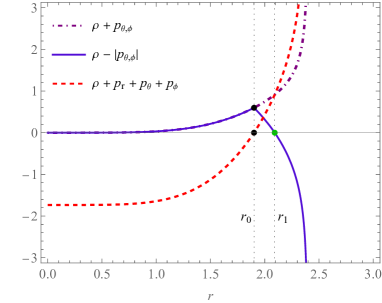
Figure 1: The radial profiles of the values in Eqs. (17) are plotted for $\mathcal{B}=0.03$, $\alpha=0.6$, $\mathcal{k}=0.4$, $q=10$, and $\rho_{0}=10$. The quantity $\rho+p_{\theta,\phi}$ remains positive throughout the domain, while $\rho+p_{r}+p_{\theta}+p_{\phi}$ shifts from negative to positive at $r_{0}=1.901$, denoted by black points. This transition point corresponds to the sign change of $p_{\theta,\phi}$ from attractive to repulsive, where $\rho-|p_{\theta,\phi}|$ shifts from ascending to descending, until it finally enters the domain of negative values at $r_{1}=2.092$ (the green point).

Based on the behavior of these quantities, one can infer the following:

$$\rho+p_{\theta,\phi}\geq 0\quad\Longrightarrow\quad\text{NEC and WEC are satisfied},$$ (18a)

$$\rho+\sum_{i=r,\theta,\phi}p_{i}\left\{\begin{array}[]{cc}\leq 0\quad\text{for}\quad r\leq r_{0}\quad\Longrightarrow\quad\text{SEC is violated,}\\ >0\quad\text{for}\quad r>r_{0}\quad\Longrightarrow\quad\text{SEC is satisfied,}\end{array}\right.$$ (18d)

$$\rho-|p_{\theta,\phi}|\left\{\begin{array}[]{cc}\geq 0\quad\text{for}\quad r\leq r_{1}\quad\Longrightarrow\quad\text{DEC is satisfied,}\\ <0\quad\text{for}\quad r>r_{1}\quad\Longrightarrow\quad\text{DEC is violated.}\end{array}\right.$$ (18g)

Note that, having both repulsive gravitational effects and obeying the SEC is not inherently contradictory in general relativity. The SEC mainly ensures that gravity overall pulls things together. However, when the DEC is violated, it means certain types of energy, like dark energy, become dominant, leading to repulsive gravitational effects, especially at large distances. This fits with what we observe in the universe’s expansion. For instance, in some cosmological models with exotic matter like phantom energy, we see both SEC compliance and DEC violation, causing the universe’s expansion to speed up in unexpected ways. As declared in Ref. [67], the SEC is obeyed by the matter source in deflationary models, but it is violated during the early evolution of the cosmos in such models, allowing for the avoidance of the initial singularity. Conversely, violation of the DEC corresponds to the violation of the generalized second law of thermodynamics in general relativity. However, such violation does not necessarily invalidate a given cosmological model (see, e.g., Ref. [68]). Similarly, violation of the SEC is not in contrast with ordinary inflationary models [69]. In general, violation of the DEC is attributed to the bulk viscous stress as a result of particle production [67, 70, 71, 72]. However, situations where the SEC is satisfied while the DEC is violated are not difficult to find. An example would be during the transition from the Schwarzschild vacuum to de Sitter spacetime, as discussed in Ref. [73]. Based on the above notes, it is reasonable to anticipate the presence of an exotic field outside the Schwarzschild radius at $r_{s}=2$ in our model.

Now, substitution of the expression (14) in the differential equation (12) results in the (anti-)de Sitter-like (Ads-like) lapse function

$$f(r)=1-\frac{2M}{r}-\frac{1}{3}\lambda(r)r^{2},$$ (19)

where the function $\lambda(r)$ is

$$\lambda(r)=\rho_{0}\left[\frac{\mathcal{B}\bigr{(}1+y(r)\bigr{)}\bigr{(}\mathcal{k}y(r)-\mathcal{k}^{\prime}\bigr{)}}{1+\frac{\mathcal{k}}{\mathcal{k}^{\prime}}y(r)}\right]^{\frac{1}{1+\alpha}}\times F_{1}\left(-\frac{1}{1+\alpha};-\frac{1}{1+\alpha},\frac{1}{1+\alpha};\frac{\alpha}{1+\alpha};\frac{\mathcal{k}}{\mathcal{k}^{\prime}}y(r),-y(r)\right),$$ (20)

in which, $F_{1}(a;b_{1},b_{2};z;x_{1},x_{2})$ represents the two-variable Appell hypergeometric function. The integration constant in Eq. (19) is set to $2M$ to retrieve the Schwarzschild solution component (by setting $\rho_{0}=0$ or $\mathcal{B}=0$), where $M$ denotes the black hole mass. It is important to note that we cannot recover the CDF solution at the limit of $\alpha=1=\mathcal{k}$, as this solution is well-defined only for $\mathcal{k}^{\prime}\neq 0$. To retrieve that solution, one would need to start from the corresponding EoS and the density profile. In fact, the Appell function in Eq. (20) can be transformed as [74]

$$F_{1}\left(-\frac{1}{1+\alpha};-\frac{1}{1+\alpha},\frac{1}{1+\alpha};\frac{\alpha}{1+\alpha};\frac{\mathcal{k}}{\mathcal{k}^{\prime}}y(r),-y(r)\right)\\ =\left[1-\frac{\mathcal{k}}{\mathcal{k}^{\prime}}y(r)\right]^{\frac{1}{1+\alpha}}F_{1}\left(-\frac{1}{1+\alpha};\frac{\alpha}{1+\alpha},\frac{1}{1+\alpha};\frac{\alpha}{1+\alpha};\frac{y(r)}{\mathcal{k}y(r)-\mathcal{k}^{\prime}},\frac{y(r)}{\mathcal{k}y(r)-\mathcal{k}^{\prime}}\right)\\ =\left[1-\frac{\mathcal{k}}{\mathcal{k}^{\prime}}y(r)\right]^{\frac{1}{1+\alpha}}\,_{2}F_{1}\left(1,-\frac{1}{\alpha+1};\frac{\alpha}{\alpha+1};\frac{y(r)}{\mathcal{k}y(r)-\mathcal{k}^{\prime}}\right),$$ (21)

in which ${}_{2}F_{1}(a,b;z,x)$ is the Gaussian hypergeometric function. Based on the inclusion of the simpler hypergeometric function in this relation, the computational time for numeric processes is significantly reduced. Consequently, the form presented in Eq. (21) will be considered for further studies. In Fig. 2, the radial profile of the lapse function (19) has been plotted for some values of the parameter $\mathcal{B}$. As expected, the Schwarzschild black hole with $\mathcal{B}=0$ shows the largest values for the lapse function. On the other hand, the GCJDF black hole possesses two horizons; the event horizon $r_{+}$ (where the infinite redshift occurs), and the cosmological horizon $r_{++}$ (where the infinite blueshift occurs). Accordingly, the lapse function has an extremum and its value decreases by the increase in the $\mathcal{B}$-parameter.

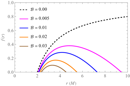
Figure 2: The radial profile of the lapse function of the GCJDF black hole plotted for $\alpha=0.6$, $q=0.1$, $\mathcal{k}=0.4$, $\rho_{0}=1$, and various values of the $\mathcal{B}$-parameter. The dashed curve corresponds to the case of the Schwarzschild black hole with $\mathcal{B}=0$. In this diagram and all subsequent ones within this paper, the unit of length along the axes is considered as the black hole mass $M$.

Before proceeding with further studies on the GCJDF black hole, it is worth mentioning that for small values of $\alpha$, where $\alpha+1\approx 1$, the hypergeometric function in Eq. (20) can be simplified to

$$F_{1}\left(-\frac{1}{1+\alpha};-\frac{1}{1+\alpha},\frac{1}{1+\alpha};\frac{\alpha}{1+\alpha};\frac{\mathcal{k}}{\mathcal{k}^{\prime}}y(r),-y(r)\right)\approx 1+\frac{q^{2}}{\alpha\mathcal{k}^{\prime}r^{3}},$$ (22)

by taking into account the approximation $y(r)\approx q^{2}r^{-3}$ for $\alpha\ll 1$. In this limit, therefore, the parameter $\lambda(r)$ in Eq. (20) is approximated as

$$\lambda(r)\approx\frac{\text{{\hbox{\rho_0}}}\mathcal{B}\left(q^{2}+r^{3}\right)\left(\mathcal{k}q^{2}-\mathcal{k}^{\prime}r^{3}\right)\left(q^{2}+\alpha\mathcal{k}^{\prime}r^{3}\right)}{\alpha r^{6}\left(\mathcal{k}^{\prime}r^{3}+\mathcal{k}q^{2}\right)}+\mathcal{O}(\alpha^{2}).$$ (23)

In Fig. 3, the radial profile of the lapse function $f(r)$ has been plotted, by considering the cosmological parameter in Eq. (23).

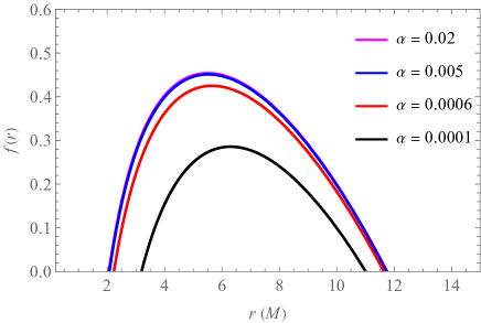
Figure 3: The radial profile of the reduced lapse function with the cosmological parameter given in Eq. (23), plotted for $\mathcal{B}=0.03$, $q=0.1$, $\mathcal{k}=0.4$, $\rho_{0}=1$, and some small values of the $\alpha$-parameter.

One can observe from the profiles that, for $\alpha>0.001$, the changes in the maximum of $f(r)$ is not great. This domain is also more reliable for the condition $\alpha+1\approx 1$, for which, $\alpha$ is still have values notably larger than zero. We can therefore infer that for this limit, the alternations in the black hole spacetime, receive more contributions from changes in the $\mathcal{B}$-parameter.

It is also important to note that besides the natural curvature singularity at $r=0$, there is another singularity occurring at

$$r_{*}=\left(\frac{\mathcal{k}q^{2}}{\mathcal{k}^{\prime}}\right)^{\frac{1}{3(\alpha+1)}},$$ (24)

at which $f(r)$ diverges. It is, in general, required that the curvature singularity be located inside the event horizon, in other words, $r_{*}<r_{+}$, which is respected by the GCJDF black hole. Let us now select a Bondi coordinate $v$ such that it aligns with the center of mass Bondi cuts in the limit $v\rightarrow\infty$. This choice pertains to the past of an open set of future null infinity $\mathcal{J}^{+}$, defined by points whose Bondi retarded time is defined in the domain $v\in(v_{0},\infty)$ [75]. The null geodesic congruence, defined by $\tilde{\ell}=\mathrm{d}v$ permits the introduction of the affine parameter $r$, which in our black hole spacetime serves as the radial coordinate. This parameter is chosen such that it asymptotically matches the luminosity distance. The surfaces $(v,r)=\mathrm{const.}$ represent spheres, inheriting natural spherical coordinates from the Bondi cuts at $\mathcal{J}^{+}$, which label null rays of the congruence. Collectively, these elements establish a coordinate system $(v,r,x^{A})$, with $x^{A}$ denoting coordinates on the two-dimensional sphere $S^{2}$ [75]. This way, the line element of the GCJDF black hole can be recast as

$$\mathrm{d}s^{2}=-f(r)\mathrm{d}v+2\mathrm{d}v\mathrm{d}r+r^{2}\left(\mathrm{d}\theta^{2}+\sin^{2}\theta\mathrm{d}\phi^{2}\right),$$ (25)

in the Bondi coordinates, possessing the time-like Killing vector $\xi^{\mu}=(1,0,0,0)$. Accordingly, if the above line element is applied, we obtain $\xi_{\mu}=\big{(}f(r),1,0,0\big{)}$. Now to obtain the surface gravity of the hypersphere corresponding to the black hole event horizon, we re-call the relation ${\xi^{\mu}}_{;\nu}\xi^{\nu}=\kappa\xi^{\mu}$ as the non-affinely parametrized geodesics equations, in which $\kappa$ is the surface gravity [76, 77]. Applying the metric (25), this equation results in

$$\kappa_{+}=\frac{1}{2}f^{\prime}(r_{+}),$$ (26)

as the surface gravity of the black hole on its event horizon. Hence, the corresponding Hawking temperature of the GCJDF is obtained as $T_{\mathrm{H}}^{+}=\kappa_{+}/(2\pi)$. In Fig. 4, the $\mathcal{B}$-profile of the Hawking temperature of the GCJDF black hole has been demonstrated, for some different values of the $\alpha$-parameter. This diagram has been obtained by generating the triplet $\{\mathcal{B},r_{+},T_{\mathrm{H}}^{+}\}$, for fixed values for the other parameters.

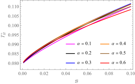
Figure 4: The $\mathcal{B}$-profile of the Hawking temperature on the event horizon, $T^{+}_{\mathrm{H}}$, for different values of the $\alpha$-parameter, considering $q=0.1$, $\mathcal{k}=0.4$ and $\rho_{0}=1$.

The plot shows the variation of $T_{\mathrm{H}}^{+}$ with respect to $\mathcal{B}$ for different values of $\alpha$. Starting from the Schwarzschild black hole (i.e. $\mathcal{B}=0$), $T_{\mathrm{H}}^{+}$ rises with increasing $\mathcal{B}$. It is evident that as $\alpha$ rises, the rate of increase in $T_{\mathrm{H}}^{+}$ with respect to $\mathcal{B}$ also escalates.

Now that the general structure of the black hole in the GCJDF has been identified, we commence our investigation on the properties of this black hole from the next section.

IV General formalism for shadow formation and light deflection angle

In the presence of a black hole, light emitted from a source may undergo deflection due to the gravitational field of the black hole before reaching an observer. This deflection can lead to the formation of a shadow, where some photons are absorbed by the black hole, creating a region devoid of light. The boundary of this shadow defines the apparent shape of the black hole. Here, we review the general equations required to calculate the shape of the shadow, the energy emission rate, and the deflection angle. These formulas are derived for the general ansatz (3) for the case of $f(r)=g(r)$, necessitating an examination of test particle motion within the spacetime.

IV.1 The equations of motion for light rays

Pursuing the standard Lagrangian method in the study of test particle motion in gravitational fields, let us write the Lagrangian [78]

$$\mathcal{L}=\frac{1}{2}g_{\mu\nu}\dot{x}^{\mu}\dot{x}^{\mu},$$ (27)

in which the overdot represents differentiation with respect to the affine parameter of the geodesic curves, denoted as $\tau$. This way, the components of the canonically conjugate momentum can be defined as

$$p_{t}=f(r)\dot{t}=E,$$ (28)

$$p_{r}=\frac{\dot{r}}{f(r)},$$ (29)

$$p_{\theta}=r^{2}\dot{\theta},$$ (30)

$$p_{\phi}=r^{2}\sin^{2}\theta\dot{\phi}=L,$$ (31)

in which $E$ and $L$ are, respectively, the energy and the angular momentum associated to the test particles. This way, the Hamilton-Jacobi equation can be written as [79]

$$\frac{\partial\mathcal{S}}{\partial\tau}=-\frac{1}{2}g^{\mu\nu}\frac{\partial\mathcal{S}}{\partial x^{\mu}}\frac{\partial\mathcal{S}}{\partial x^{\nu}},$$ (32)

where $\mathcal{S}$ is the Jacobi action. Taking into account the ansatz (3) in the above equation, we can recast the Hamilton-Jacobi equation as

$$-2\frac{\partial\mathcal{S}}{\partial\tau}=-\frac{1}{f(r)}\left(\frac{\partial\mathcal{S}_{t}}{\partial t}\right)^{2}+{f(r)}\left(\frac{\partial\mathcal{S}_{r}}{\partial r}\right)^{2}+\frac{1}{r^{2}}\left(\frac{\partial\mathcal{S}_{\theta}}{\partial\theta}\right)^{2}+\frac{1}{r^{2}\sin^{2}\theta}\left(\frac{\partial\mathcal{S}_{\phi}}{\partial\phi}\right)^{2}.$$ (33)

Based on the method of the separation of variables, and considering the constants of motion defined earlier, the Jacobi action can be expressed as

$$\mathcal{S}=\frac{1}{2}m^{2}\tau-Et+L\phi+\mathcal{S}_{r}(r)+\mathcal{S}_{\theta}(\theta),$$ (34)

with $m$ being the rest mass of the test particles. Since in this study we are dealing with photons, we hence set $m=0$. Now using Eq. (34) in Eq. (33), we get

$$0=\frac{E^{2}}{f(r)}-f(r)\left(\frac{\partial\mathcal{S}_{r}}{\partial r}\right)^{2}-\frac{1}{r^{2}}\left[\frac{L^{2}}{\sin^{2}\theta}+\mathscr{Q}-L^{2}\cot^{2}\theta\right]-\frac{1}{r^{2}}\left[\left(\frac{\partial\mathcal{S}_{\theta}}{\partial\theta}\right)^{2}-\mathscr{Q}+L^{2}\cot^{2}\theta\right],$$ (35)

where $\mathscr{Q}$ is the Carter’s constant. This way, the following two equations are obtained:

$$r^{4}f(r)^{2}\left(\frac{\partial\mathcal{S}_{r}}{\partial r}\right)^{2}=r^{4}E^{2}-r^{2}\left(L^{2}+\mathscr{Q}\right)f(r),$$ (36)

$$\left(\frac{\partial\mathcal{S}_{\theta}}{\partial\theta}\right)^{2}=\mathscr{Q}-L^{2}\cot^{2}\theta.$$ (37)

By applying Eq. (28)–(31) to the above equations, we get to the full set of equations of motion for null geodesics as

$$\dot{t}=\frac{E}{f(r)},$$ (38)

$$\dot{r}=\pm\frac{\sqrt{\mathcal{R}(r)}}{r^{2}},$$ (39)

$$\dot{\theta}=\pm\frac{\sqrt{\Theta(\theta)}}{r^{2}},$$ (40)

$$\dot{\phi}=\frac{L}{r^{2}\sin^{2}\theta},$$ (41)

in which the $+\,(-)$ sign corresponds to the outgoing (ingoing) nature of the trajectories. In the above relations, we have defined the variables

$$\mathcal{R}(r)=r^{4}E^{2}-r^{2}\left(L^{2}+\mathscr{Q}\right)f(r),$$ (42a)

$$\Theta(\theta)=\mathscr{Q}-L^{2}\cot^{2}\theta.$$ (42b)

Note that, by considering the definition (42a), we can recast Eq. (39) as

$$\dot{r}^{2}+V(r)=0,$$ (43)

in which

$$V(r)=\frac{f(r)}{r^{2}}\left(L^{2}+\mathscr{Q}\right)-E^{2},$$ (44)

is the effective potential for the null geodesics. Indeed, photons approaching the black hole may either deflect from it or plunge onto the event horizon. These potential outcomes for photons can be predicted by considering their initial energy and angular momentum in the gravitational effective potential. Furthermore, the point at which photons reach the threshold between these two fates corresponds to the maximum of this effective potential, which can be determined based on specific criteria

$$V(r_{p})=V^{\prime}(r_{p})=0,\qquad\mathcal{R}(r_{p})=\mathcal{R}^{\prime}(r_{p})=0.$$ (45)

Here, $r_{p}$ denotes the radius of the photon sphere around the black hole, where photons reside in a state of instability. Therefore, one can deduce that the radius of the photon sphere can be determined as the smallest root of the equation

$$r_{p}f^{\prime}(r_{p})-2f(r_{p})=0.$$ (46)

IV.2 Shadow parametrization

The test particle geodesics can be identified by the two impact parameters [80, 78]

$$\xi=\frac{L}{E},$$ (47)

$$\eta=\frac{\mathscr{Q}}{E^{2}}.$$ (48)

Accordingly, one can recast

$$V(r)=E^{2}\left[\frac{f(r)}{r^{2}}\left(\eta+\xi^{2}\right)-1\right],$$ (49)

$$\mathcal{R}(r)=E^{2}r^{2}\left[r^{2}-f(r)\left(\eta+\xi^{2}\right)\right].$$ (50)

Hence, the conditions (45) provide the expressions

$$\xi_{p}^{2}(r_{p})=\frac{r_{p}^{2}\left[2f(r_{p})-r_{p}f^{\prime}(r_{p})\right]}{2f(r_{p})\left[2f(r_{p})+r_{p}f^{\prime}(r_{p})\right]},$$ (51)

$$\eta_{p}(r_{p})=\frac{r_{p}^{2}\left[6f(r_{p})+r_{p}f^{\prime}(r_{p})\right]}{2f(r_{p})\left[2f(r_{p})+r_{p}f^{\prime}(r_{p})\right]},$$ (52)

that satisfy the relationship

$$\eta_{p}+\xi_{p}^{2}=\frac{4r_{p}^{2}}{2f(r_{p})+r_{p}f^{\prime}(r_{p})},$$ (53)

on the photon sphere. As mentioned earlier, the photon sphere is formed by photons on unstable orbits. In fact, photons orbiting on the unstable trajectories within the gravitational field of black holes will either plunge into the event horizon or escape from it. Those that escape, form a luminous photon ring that encapsulates the shadow of the black hole [81, 82, 83, 84]. Notably, Luminet’s optical simulation of a Schwarzschild black hole and its accretion in 1979 [84] provided deeper insights into these photon rings, originating from the highly distorted region around black holes. The resulting formulations aided scientists in confining the shadow of rotating black holes within their respective photon rings. Subsequently, Bardeen developed mathematical techniques to compute the shape and size of a Kerr black hole’s shadow [85, 83, 80], later refined and applied by Chandrasekhar [78]. These methods were further expanded and generalized extensively (see Refs. [86, 87, 88, 89, 90, 91]). With these tools, rigorous analytical calculations, simulations, numerical and observational studies were conducted on a multitude of black hole spacetimes, including those with cosmological components [92, 93, 94, 95, 96, 97, 98, 99, 100, 101, 102, 103, 104, 105, 106]. The black hole shadow is of significant importance as it offers insights into light propagation in the vicinity of the horizon. Recent investigations have aimed to establish relationships between the shadow and black hole parameters (see, e.g., Refs. [107, 108] for thermodynamic aspects and Refs. [109, 110, 111, 112, 113, 114, 115, 116] for dynamical aspects of black hole shadows). To determine the shadow of the GCJDF black hole, we must consider that this spacetime is not asymptotically flat. Hence, the traditional approach of considering an observer at infinity, as done in Refs. [83, 80] and Ref. [87], cannot be applied. Instead, an observer is located at the coordinate position $(r_{o},\theta_{o})$, characterized by the orthonormal tetrad $\bm{e}_{\{A\}}$, expressed as

$$\bm{e}_{0}=\left.\frac{1}{\sqrt{f(r)}}\,\partial_{t}\right|_{(r_{o},\theta_{o})},$$ (54a)

$$\bm{e}_{1}=\left.\frac{1}{r}\,\partial_{\theta}\right|_{(r_{o},\theta_{o})},$$ (54b)

$$\bm{e}_{2}=\left.-\frac{\csc\theta}{r}\,\partial_{\phi}\right|_{(r_{o},\theta_{o})},$$ (54c)

$$\bm{e}_{3}=\left.-\sqrt{f(r)}\,\partial_{r}\right|_{(r_{o},\theta_{o})},$$ (54d)

which satisfy the condition ${{e}_{A}}^{\mu}{{e}^{B}}_{\mu}=\delta^{B}_{A}$. The method, initially proposed in Ref. [88], facilitates the computation of celestial coordinates in spacetimes featuring cosmological constituents (also discussed in Ref. [89]). Within the aforementioned set of tetrads, the time-like vector $\bm{e}_{0}$ serves as the velocity four-vector of the chosen observer. Additionally, $\bm{e}_{3}$ is oriented towards the black hole, and $\bm{e}_{0}\pm\bm{e}_{3}$ generates the principal null congruence. Consequently, a linear combination of $\bm{e}_{\{A\}}$ aligns with the tangent to the light ray $\bm{\ell}(\tau)=\left(t(\tau),r(\tau),\theta(\tau),\phi(\tau)\right)$, originating from the black hole and extending into the past. This tangent can be parametrized in the two distinct ways

$$\dot{\bm{\ell}}={\dot{t}}{}\,\partial_{t}+{\dot{r}}\,\partial_{r}+{\dot{\theta}}\,\partial_{\theta}+{\dot{\phi}}\,\partial_{\phi},$$ (55)

$$\dot{\bm{\ell}}=-\frac{E}{\sqrt{f(r)}}\bigl{(}-\bm{e}_{0}+\sin\vartheta\cos\psi\,\bm{e}_{1}+\sin\vartheta\sin\psi\,\bm{e}_{2}+\cos\vartheta\,\bm{e}_{3}\bigr{)},$$ (56)

in which $\vartheta$ and $\psi$ represent newly defined celestial coordinates in the observer’s sky. It is evident that $\vartheta=0$ directly aligns with the black hole’s axis. As the boundary curve of the shadow arises from light rays intersecting the unstable (critical) null geodesics at the radial distance $r_{p}$, this region corresponds to the critical impact parameters $\xi_{p}$ and $\eta_{p}$, as given in Eqs. (51) and (52). The respective celestial coordinates $(\psi_{p},\vartheta_{p})$ at this distance, for an observer positioned at $(r_{o},\theta_{o})$, have been derived in Ref. [88] as

$$\mathcal{P}(r_{p},\theta_{o})\vcentcolon=\sin\psi_{p}=\frac{\csc\theta_{o}\,\xi_{p}(r_{p})}{\sqrt{\eta_{p}(r_{p})}},$$ (57)

$$\mathcal{T}(r_{p},r_{o})\vcentcolon=\sin\vartheta_{p}=\frac{1}{r_{o}}{\sqrt{f(r_{o})\,\eta_{p}(r_{p})}}.$$ (58)

Hence, the $\vartheta$-coordinate attains its maximum and minimum values for $\psi_{p}=-\pi/2$ and $\psi_{p}=\pi/2$, respectively. Now, The two-dimensional Cartesian coordinates for the chosen observer of the velocity four-vector $\bm{e}_{0}$ are obtained by applying the stereographic projection of the celestial sphere $(\psi_{p},\vartheta_{p})$ onto a plane. This yields the coordinates [88]

$$X_{p}=-2\tan\left(\frac{\vartheta_{p}}{2}\right)\sin\psi_{p},$$ (60)

$$Y_{p}=-2\tan\left(\frac{\vartheta_{p}}{2}\right)\cos\psi_{p}.$$

The case of $\theta_{o}=\pi/2$ depicts an edge-on view of the shadow, while $\theta_{o}=0$ represents a face-on perspective. Although the case of $\theta_{o}=0$ is not well-defined in the coordinate $\psi_{p}$ as seen in Eq. (57), it is irrelevant in the context of our static black hole. In such a scenario, there would be no distinction between the edge-on and face-on views. Thus, we can proceed with the case of $\theta_{o}=\pi/2$ without considering this issue further. Using Eqs. (60) and (60), along with the definitions in (57) and (58), we can derive the expression

$$R_{s}=\sqrt{X_{p}^{2}+Y_{p}^{2}}=2\tan\left(\frac{1}{2}\arcsin\left(\frac{\sqrt{f(r_{o})\,\eta_{p}(r_{p})}}{r_{o}}\right)\right).$$ (61)

Since the black hole is static, the photon ring in the observer’s sky would appear as a circle with a radius of $R_{s}$, as defined in the equation above.

IV.3 The energy emission rate

At high energy levels, Hawking radiation is typically emitted within a finite cross-sectional area, denoted as $\sigma_{l}$. For distant observers positioned far from the black hole, this cross-section gradually approaches the shadow cast by the black hole [117, 118]. It has been shown that $\sigma_{l}$ is directly linked to the area of the photon ring and can be mathematically represented as [118, 119, 120]

$$\sigma_{l}\approx\pi R_{s}^{2}.$$ (62)

Accordingly, the energy emission rate of the black hole can be expressed as

$$\Omega\equiv\frac{\mathrm{d}^{2}E(\varpi)}{\mathrm{d}\varpi\,\mathrm{d}t}=\frac{2\pi^{2}\sigma_{l}}{e^{\varpi/T_{\mathrm{H}}^{+}}-1}\,\varpi^{3},$$ (63)

in which $\varpi$ is the emission frequency.

IV.4 The Deflection angle

Gravitational lensing has emerged as a powerful tool for astrophysicists, offering a unique window into the universe. The phenomenon, caused by the bending of light around massive bodies, has facilitated numerous scientific breakthroughs since the advent of general relativity. In particular, significant progress has been made in the past two decades in developing theoretical frameworks for calculating deflection angles and predicting lensing effects on the images of astrophysical objects (see, e.g., the seminal works in Refs. [121, 122, 123, 124, 125, 126, 127]). As an alternative approach, in this subsection, we introduce the general methodology for calculating the deflection of light angles by static spherically symmetric black holes, employing the GBT as described in Refs. [128, 129]. To begin, we restrict our analysis to the equatorial plane (i.e., setting $\theta=\pi/2$ in the line element (3)). Consequently, the Jacobi metric takes the form

$$\mathrm{d}l^{2}=-f(r)\mathrm{d}t^{2}+\frac{\mathrm{d}r^{2}}{f(r)}+r^{2}\mathrm{d}\phi^{2},$$ (64)

which reduces to the optical metric

$$\mathrm{d}t^{2}=\frac{\mathrm{d}r^{2}}{f(r)^{2}}+\frac{r^{2}}{f(r)}\,\mathrm{d}\phi^{2},$$ (65)

for the null geodesics where $\mathrm{d}l=0$. Calculating the Ricci scalar $\mathfrak{R}$ of this metric, one can then calculate the Gaussian curvature of the optical metric as

$$\mathcal{K}=\frac{\mathfrak{R}}{2}=f(r)f^{\prime\prime}(r)-\frac{1}{2}f^{\prime}(r)^{2}.$$ (66)

In the approach outlined in Ref. [128], calculating the deflection angle involves considering a non-singular domain $(\mathcal{D},\chi,\bm{g})$ as a subset of an oriented Riemannian surface characterized by the Euler characteristic $\chi$ and the metric $\bm{g}$, with a relevant Gaussian curvature $\mathcal{K}$. If the boundary of this domain, denoted by $\partial\mathcal{D}$, possesses a geodesic curvature $\mathcal{C}$, then the GBT can be expressed as [130, 131]

$$\int\int_{\mathcal{D}}\mathcal{K}\,\mathrm{d}S+\int_{\partial\mathcal{D}}\mathcal{C}~{}\mathrm{d}t+\sum_{i}\theta_{i}=2\pi\chi(\mathcal{D}),$$ (67)

in which, $\mathrm{d}S$ represents the infinitesimal area element of $\mathcal{D}$, $\theta_{i}$denotes the exterior angle at the $i$th vertex, and $\chi(\mathcal{D})=1$ since $\mathcal{D}$ is non-singular. Here, a smooth congruence $\bm{\gamma}:\{t\}\rightarrow\mathcal{D}$ of unit speed, denoted by $\bm{g}(\dot{\bm{\gamma}},\dot{\bm{\gamma}})\equiv\dot{\bm{\gamma}}\cdot\dot{\bm{\gamma}}=1$, along with its acceleration $\ddot{\bm{\gamma}}$, forms a Frenet frame. Consequently, the geodesic curvature of $\bm{\gamma}$ is expressed as [130]

$$\mathcal{C}=\bm{g}(\nabla_{\dot{\bm{\gamma}}}\dot{\bm{\gamma}},\ddot{\bm{\gamma}}),$$ (68)

which vanishes iff $\bm{\gamma}$ is a geodesic congruence. We assume that the observer $\mathbb{O}$ at the interior angle $\theta_{\mathbb{O}}$, the lens $\mathbb{L}$, and the source $\mathbb{S}$ at $\theta_{\mathbb{S}}$, are located on the same two-dimensional surface. Then these two angles sum up to

$$\theta_{\mathbb{O}}+\theta_{\mathbb{S}}=\int\int_{\mathcal{D}_{1}}\mathcal{K}\,\mathrm{d}S,$$ (69)

where $\mathcal{D}_{1}$ is a non-singular subspace of $\mathcal{D}$ bounded by the geodesics connecting $\mathbb{S}$ to $\mathbb{O}$. In Ref. [132], it has been proven that for a static spherically symmetric spacetime with the optical metric given by Eq. (65), the deflection angle can be determined using Eq. (69), which yields

$$\hat{\upsilon}=\int\int_{{}_{\mathbb{O}}\Delta^{\mathbb{S}}_{\mathbb{L}}}\mathcal{K}\,\mathrm{d}{S},$$ (70)

where ${}_{\mathbb{O}}\Delta^{\mathbb{S}}_{\mathbb{L}}$ represents the triangle formed by the observer, the lens, and the source. Based on the characteristics of the spacetime being studied, this can be reformulated as

$$\hat{\upsilon}=\int_{0}^{\pi}\int_{r_{\mathrm{c}}}^{r_{\mathbb{O}}}\mathcal{K}\,\mathrm{d}S,$$ (71)

in which, $r_{\mathrm{c}}=\xi/\sin\phi$ denotes the distance of closest approach, and $\mathrm{d}S=\sqrt{\mathfrak{g}}\,\mathrm{d}r\mathrm{d}\phi$, with $\mathfrak{g}=r^{2}f(r)^{-3}$ representing the determinant of the optical metric (65).

In the following section, we apply the formulations introduced in this section to the GCJDF black hole to calculate the geometrical shapes of the shadow and the deflection angle. Additionally, we propose constraints on the black hole parameters based on the outcomes of the EHT.

V Shadow and the deflection angles of the GCJDF black hole

In this section, we examine the shadow and deflection angle of the GCJDF black hole by employing the framework outlined in the previous section. Our objective is to analyze how various factors such as the $\mathcal{B}$-parameter influence the behavior of the shadow and deflection angle. Specifically, we apply the line element corresponding to the black hole to the derived formulas within our framework. Through this investigation, we aim to determine how the shadow behavior of the black hole is sensitive to changes in the intrinsic black hole parameters.

V.1 The effective potential

To obtain the exact expression for the effective potential, let us exploit Eqs. (19), (20) and (21), in Eq. (44), which provide

$$V(r)=\frac{\left(L^{2}+\mathscr{Q}\right)(r-2M)}{r^{3}}-E^{2}-\frac{1}{3}\rho_{0}\left(L^{2}+\mathscr{Q}\right)\left[1-\frac{\mathcal{k}q^{2}r^{-3(\alpha+1)}}{\mathcal{k}^{\prime}}\right]^{\frac{1}{\alpha+1}}\\ \times\left[\frac{\mathcal{k}^{\prime}\mathcal{B}\left(q^{2}+r^{3\alpha+3}\right)\left(\mathcal{k}q^{2}-\mathcal{k}^{\prime}r^{3\alpha+3}\right)}{\mathcal{k}q^{2}r^{3\alpha+3}+\mathcal{k}^{\prime}r^{6\alpha+6}}\right]^{\frac{1}{\alpha+1}}{}_{2}F_{1}\left(1,-\frac{1}{\alpha+1};\frac{\alpha}{\alpha+1};\frac{1}{\mathcal{k}-\frac{\mathcal{k}^{\prime}r^{3\alpha+3}}{q^{2}}}\right).$$ (72)

In Fig. 5, the radial profile of the effective potential has been plotted for different values of the black hole parameters.

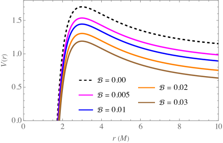
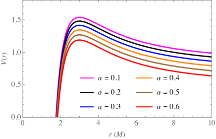
(a)  (b)

Figure 5: The radial profile of the effective potential plotted for $\mathcal{k}=0.4$, $q=0.1$, $\rho_{0}=1$, $\mathscr{Q}=10$, $E=1$, $L=3$, and (a) five different values of the $\mathcal{B}$-parameter while $\alpha=0.6$, and (b) six different values of the $\alpha$-parameter while $\mathcal{B}=0.03$.

Observing the diagrams, it is evident that variations in the $\mathcal{B}$-parameter yield more noticeable effects compared to alterations in the $\alpha$-parameter, as indicated by the greater separation between the peaks of the effective potential. From the right panel of the figure, we observe that an increase in the $\alpha$-parameter lowers the peak of the effective potential. This indicates that as the dark fluid becomes less anisotropic, the black hole’s tendency to bend light decreases, resulting in fewer deflecting trajectories. This phenomenon will be further emphasized in Subsect. V.4, where the deflection angles are analyzed. Additionally, it is noteworthy that the Schwarzschild black hole dominates the highest photon energies, given its larger effective potential’s peak. Notably, alterations in other spacetime parameters do not significantly alter the overall behavior of the effective potential. Particularly, the parameter $\rho_{0}$ serves as a scaling factor; lower values of $\rho_{0}$ correspond to higher peaks in the effective potential. Nonetheless, the Schwarzschild black hole consistently serves as an upper limit across all cases of the GCJDF black hole.

V.2 Black hole shadow

Applying the formulation provided in Subsect. IV.2, we can characterize the outer boundary of the black hole shadow, referred to as the critical curve. To do this, we utilize the impact parameter from Eq. (52) for specific values of the black hole parameters, enabling the calculation of the shadow radius $R_{s}$ in Eq. (61). In Table 2, some exemplary values of $r_{+}$, $r_{p}$ and $R_{s}$ are provided for various cases of intrinsic black hole parameters.

	$\mathcal{B}=0.00$			$\mathcal{B}=0.005$			$\mathcal{B}=0.01$			$\mathcal{B}=0.02$			$\mathcal{B}=0.03$
$\alpha$	$r_{+}$	$r_{p}$	$R_{s}$	$r_{+}$	$r_{p}$	$R_{s}$	$r_{+}$	$r_{p}$	$R_{s}$	$r_{+}$	$r_{p}$	$R_{s}$	$r_{+}$	$r_{p}$	$R_{s}$
$0.1$	2.00	3.00	5.196	2.014	3.00032	5.320	2.023	3.0006	5.440	2.052	3.00112	5.680	2.079	3.00162	5.940
$0.2$	2.00	3.00	5.196	2.022	3.00018	5.392	2.040	3.00033	5.561	2.075	3.00058	5.910	2.111	3.00082	6.290
$0.3$	2.00	3.00	5.196	2.032	3.00013	5.487	2.057	3.00023	5.724	2.104	3.00039	6.210	2.151	3.00053	6.763
$0.4$	2.00	3.00	5.196	2.045	3.0001	5.610	2.077	3.00017	5.933	2.139	3.00027	6.611	2.202	3.00037	7.430
$0.5$	2.00	3.00	5.196	2.061	3.00008	5.764	2.102	3.00013	6.198	2.182	3.0002	7.150	2.267	3.00026	8.410
$0.6$	2.00	3.00	5.196	2.079	3.00006	5.955	2.132	3.0001	6.540	2.234	3.00015	7.900	2.353	3.00019	10.016

Table 2: Values of $r_{+}$, $r_{p}$, and $R_{s}$ for the GCJDF black hole at different values of $\mathcal{B}$ and $\alpha$, with $\mathcal{k}=0.4$, $q=0.1$, and $\rho_{0}=1$.

These data are subsequently utilized in Fig. 6 to visually represent the geometric shapes of the GCJDF black hole shadow.

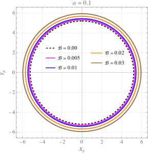
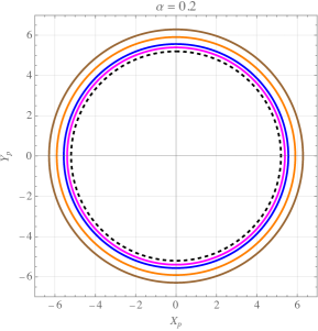
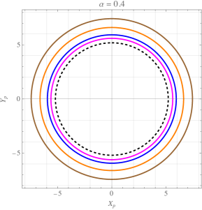
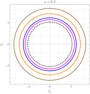
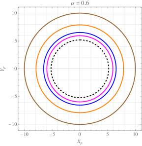
(a) (b) (c) (d) (e) (f)

Figure 6: The circles corresponding to the critical curves for the GCJDF black hole with the intrinsic parameters $\mathcal{k}=0.4$, $q=0.1$ and $\rho_{0}=1$, plotted by considering an observer located at $(100,\pi/2)$. Each panel corresponds to a different value of the $\alpha$-parameter and the curves indicate the photon ring for a specific value for the $\mathcal{B}$-parameter.

As we can observe from the diagrams, for fixed values of $\alpha$, a smaller $\mathcal{B}$-parameter results in a smaller shadow diameter. Accordingly, the Schwarzschild black hole has the smallest shadow, constituting the lower limit regarding the shadow size. Furthermore, for fixed $\mathcal{B}$, a larger $\alpha$-parameter results in a larger shadow size. This means that less-anisotropic dark fluids result in bigger black hole shadows in the observer’s sky. Moreover, for larger $\alpha$, the difference in the shadow size for different values of the $\mathcal{B}$-parameter is increased; the corresponding critical curves are more separated.

V.3 Energy emission rate

Similar to what was done in Sect. III, to find the numerical values of the Hawking temperature of the black hole, we can now use the $r_{+}$ values from Table 2. Next, the numerical values of $\sigma_{l}$ in Eq. (62) for different $\mathcal{B}$ and $\alpha$ should be determined from the shadow radius values, $R_{s}$, of the black hole. Consequently, by inserting the Hawking temperature and $\sigma_{l}$ values into Eq. (63), one can find the expressions for the energy emission rate in terms of different $\mathcal{B}$ and $\alpha$ associated with the GCJDF black hole. In Fig. 7, the profile of the energy emission rate has been plotted as a function of the emission frequency.

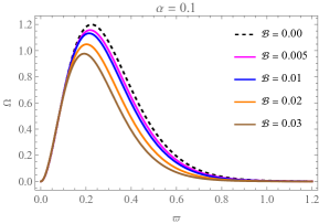
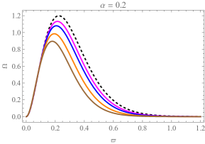
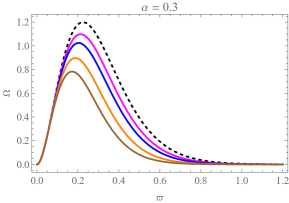
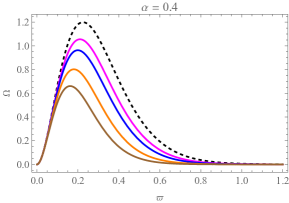
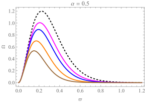
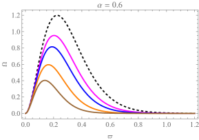
(a) (b) (c) (d) (e) (f)

Figure 7: The $\varpi$-profile of the emission frequency plotted for the data given in Table 2.

As observed from the diagrams, for all fixed values of the $\alpha$-parameter, the energy emission rate for the $\mathcal{B}=0$ case constitutes the upper limit; the Schwarzschild black hole evaporates faster, and an increase in $\mathcal{B}$ decelerates the evaporation process. Conversely, an increase in the $\alpha$-parameter, when $\mathcal{B}$ is fixed, results in lower rates of energy emission. Thus, the less anisotropic the dark fluid, the less inclined the black hole is to evaporation. Furthermore, for larger $\alpha$, the differences in the energy emission rate for different values of the $\mathcal{B}$-parameter become more noticeable.

V.4 Deflection angle

Applying the relation for the Gaussian curvature in Eq. (66) to the exterior geometry of the GCJDF black hole, we get to the following expression up to the first order in $\mathcal{B}$ and $\alpha$:

$$\mathcal{K}\approx-\frac{1}{6r^{3}}\Biggl{\{}12M\left(r^{2}+2\right)-6r^{3}+{\mathcal{B}\Biggl{[}2\rho_{0}\Biggl{(}4\mathcal{k}q^{2}\left(r^{2}+2\right)-q^{2}r^{2}+7q^{2}+\mathcal{k}^{\prime}\left(r^{2}+2\right)r^{3}\Biggr{)}\Biggr{]}}\\ +\mathcal{B}\alpha\rho_{0}\Biggl{[}q^{2}\Biggl{(}23\mathcal{k}^{2}+7\mathcal{k}^{2}r^{2}+70\mathcal{k}-10\mathcal{k}r^{2}-6\Bigl{[}4\mathcal{k}\left(r^{2}+2\right)-r^{2}+7\Bigr{]}\ln r\\ -2\Bigl{[}4\mathcal{k}\left(r^{2}+2\right)-r^{2}+7\Bigr{]}\ln(-\mathcal{B})-14+2r^{2}\Biggr{)}+\mathcal{k}^{2}r^{5}+2\mathcal{k}^{2}r^{3}-2\mathcal{k}r^{5}\\ -4\mathcal{k}r^{3}+2\mathcal{k}^{\prime}\left(r^{2}+2\right)r^{3}\ln(-\mathcal{B})\Biggr{]}\Biggr{\}}+\mathcal{O}(\alpha^{2}).$$ (73)

Using this expression in Eq. (71), the deflection angle can be estimated as

$$\hat{\upsilon}\approx\frac{\mathfrak{A}}{3\xi}+\frac{\mathfrak{B}}{3\xi^{3}}+\frac{\mathfrak{C}}{r_{\mathbb{O}}}+\frac{\mathfrak{D}}{r_{\mathbb{O}}^{3}}+\mathcal{O}\left(\frac{1}{\xi^{5}}\right),$$ (74)

in which

$$\mathfrak{A}=12M+7\alpha\mathcal{k}^{2}q^{2}\rho_{0}\mathcal{B}+6\alpha(1-4k)q^{2}\rho_{0}\mathcal{B}\ln\xi-10\alpha kq^{2}\rho_{0}\mathcal{B}-20\pi\alpha kq^{2}\rho_{0}\mathcal{B}+2\alpha(1-4k)q^{2}\rho_{0}\mathcal{B}\ln\mathcal{B}$$

$$\qquad+8\mathcal{k}q^{2}\rho_{0}\mathcal{B}+5\pi\alpha q^{2}\rho_{0}\mathcal{B}+2\alpha q^{2}\rho_{0}\mathcal{B}-2q^{2}\rho_{0}\mathcal{B},$$ (75a)

$$\mathfrak{B}=24M+23\alpha\mathcal{k}^{2}q^{2}\rho_{0}\mathcal{B}-6\alpha(8\mathcal{k}+7)q^{2}\rho_{0}\mathcal{B}\ln\xi+70\alpha\mathcal{k}q^{2}\rho_{0}\mathcal{B}-40\pi\alpha\mathcal{k}q^{2}\rho_{0}\mathcal{B}-2\alpha(8\mathcal{k}+7)q^{2}\rho_{0}\mathcal{B}\ln\mathcal{B}$$

$$\qquad+16\mathcal{k}q^{2}\rho_{0}\mathcal{B}-35\pi\alpha q^{2}\rho_{0}\mathcal{B}-14\alpha q^{2}\rho_{0}\mathcal{B}+14q^{2}\rho_{0}\mathcal{B},$$ (75b)

$$\mathfrak{C}=-2M-\frac{7}{6}\alpha k^{2}q^{2}\rho_{0}\mathcal{B}+4\alpha kq^{2}\rho_{0}\mathcal{B}\ln r_{\mathbb{O}}+\frac{5}{3}\alpha kq^{2}\rho_{0}\mathcal{B}+\frac{4}{3}\alpha kq^{2}\rho_{0}\mathcal{B}\left[\ln\mathcal{B}+\pi\right]-\frac{4}{3}kq^{2}\rho_{0}\mathcal{B}-\alpha q^{2}\rho_{0}\mathcal{B}\ln r_{\mathbb{O}}$$

$$\qquad-\frac{1}{3}\alpha q^{2}\rho_{0}\mathcal{B}-\frac{1}{3}\alpha q^{2}\rho_{0}\mathcal{B}\left[\ln\mathcal{B}+\pi\right]+\frac{1}{3}q^{2}\rho_{0}\mathcal{B},$$ (75c)

$$\mathfrak{D}=-4M-\frac{23}{6}\alpha k^{2}q^{2}\rho_{0}\mathcal{B}+8\alpha kq^{2}\rho_{0}\mathcal{B}\ln r_{\mathbb{O}}-\frac{35}{3}\alpha kq^{2}\rho_{0}\mathcal{B}+\frac{8}{3}\alpha kq^{2}\rho_{0}\mathcal{B}\left[\ln\mathcal{B}+\pi\right]-\frac{8}{3}kq^{2}\rho_{0}\mathcal{B}+7\alpha q^{2}\rho_{0}\mathcal{B}\ln r_{\mathbb{O}}$$

$$\qquad+\frac{7}{3}\alpha q^{2}\rho_{0}\mathcal{B}+\frac{7}{3}\alpha q^{2}\rho_{0}\mathcal{B}\left[\ln\mathcal{B}+\pi\right]-\frac{1}{3}7q^{2}\rho_{0}\mathcal{B}.$$ (75d)

In Fig. 8, the above relation has been applied to obtain the $\xi$-profile of the deflection angle.

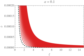
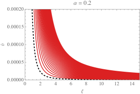
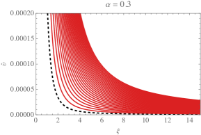
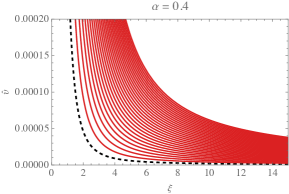
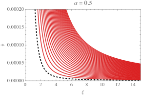
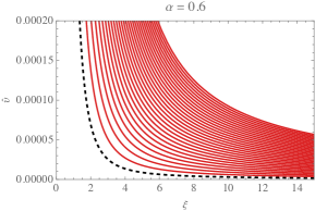
(a) (b) (c) (d) (e) (f)

Figure 8: The behavior of the deflection angle $\hat{\upsilon}$ in arcseconds regarding changes in the impact parameter $\xi$, plotted for the intrinsic parameters $\mathcal{k}=0.4$, $q=0.1$, and $\rho_{0}=1$, with an observer located at $r_{\mathbb{O}}=100$. Each panel corresponds to a specific value of the $\alpha$-parameter, and the curves indicate the behavior of the deflection angle for a range of the $\mathcal{B}$-parameter within the domain $\mathcal{B}\in(0,0.03)$, with increments of $0.001$. The dashed curve represents the case of $\mathcal{B}=0$.

As inferred from the diagrams, an increase in the $\mathcal{B}$-parameter, while keeping $\alpha$ fixed, results in the same values of the deflection angle being obtained for larger impact parameters. A similar behavior is observed for the $\mathcal{B}$-constant curves when the $\alpha$-parameter is increased; the same values of the deflection angle are achieved for larger impact parameters. Consequently, the curves fall less steeply for higher values of $\alpha$. Thus, when the fluid is less anisotropic, the black hole causes less gravitational lensing and bends light to a lesser extent. This aligns with our expectations regarding the sensitivity of the effective potential to variations in the $\alpha$-parameter, as shown in Fig. 5(b).

V.5 Observational constraints from the EHT

To enable comparisons with the EHT observations, we recall that the theoretical shadow diameter for the black hole is given by $d_{\mathrm{sh}}^{\mathrm{theo}}=2R_{s}$, where $R_{s}$ is defined in Eq. (61). To calculate the diameter of the observed shadows in the recent EHT images of M87* and Sgr A*, we use the relation [133]

$$d_{\text{sh}}=\frac{D\theta_{*}}{\gamma},$$ (76)

which calculates the shadow diameter as observed by an observer positioned at a distance $D$ (in parsecs) from the black hole. Here, $\gamma$ is the mass ratio of the black hole to the Sun. For M87*, $\gamma=(6.5\pm 0.90)\times 10^{9}$ at a distance $D=16.8\,\mathrm{Mpc}$ [11], and for Sgr A*, $\gamma=(4.3\pm 0.013)\times 10^{6}$ at $D=8.127\,\mathrm{kpc}$ [12]. In Eq. (76), $\theta_{*}$ is the angular diameter of the shadow, measured as $\theta_{*}=42\pm 3\,\mathrm{\mu as}$ for M87* and $\theta_{*}=48.7\pm 7\,\mathrm{\mu as}$ for Sgr A*. Using these values, the shadow diameters can be calculated as $d_{\mathrm{sh}}^{\mathrm{M87*}}=11\pm 1.5$ and $d_{\mathrm{sh}}^{\mathrm{SgrA*}}=9.5\pm 1.4$. These values are displayed with $1\sigma$ uncertainties for both black holes in Fig. 9, together with the $\mathcal{B}$-profile of the theoretical shadow diameter $d_{\mathrm{sh}}^{\mathrm{theo}}$. To obtain this profile, we have used Eqs. (46) and (61) to produce a set of $(\mathcal{B},2R_{s})$ points.

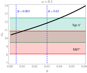
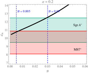
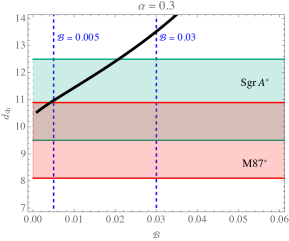
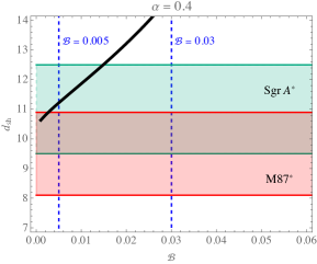
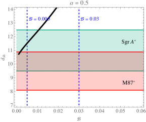
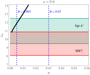
(a) (b) (c) (d) (e) (f)

Figure 9: The $\mathcal{B}$-profiles of the theoretical shadow diameter $d_{\mathrm{sh}}^{\mathrm{theo}}$ (black curves) compared with the observed shadow diameters of M87* and Sgr A*, for various values of the $\alpha$-parameter. The plots are generated for $\mathcal{k}=0.4$, $q=0.1$, and $\rho_{0}=1$.

According to the diagrams, as the $\alpha$-parameter increases, the profile tends to exit the observationally respected region. Interestingly, the initial assumed domain for the $\mathcal{B}$-parameter, which was used to generate the figures in this study, remains valid within the observational region. Based on the diagrams, it is inferred that the profile in Fig. 9(a) exhibits the most conformity with the observations. Thus, in the context of the chosen values for the other black hole parameters, the reliable range for the parameters $\alpha$ and $\mathcal{B}$ is $0<\alpha\lesssim 0.1$ and $0\leq\mathcal{B}\lesssim 0.03$, in accordance with the EHT observations.

V.6 Einstein rings

One of the interesting features of gravitational lensing due to light deflection is the formation of Einstein rings. In this subsection, we calculate the angular size of the Einstein rings formed by the black hole and examine the impact of the GCJDF and its anisotropies. Let us define the quantities $D_{\mathrm{S}}$ and $D_{\mathrm{R}}$ as the distances from the black hole (i.e., the lens) to the source and the receiver, respectively. Assuming a thin lens, the distance between the receiver and the source can be expressed as $D_{\mathrm{RS}}=D_{\mathrm{R}}+D_{\mathrm{S}}$. We then employ the lens equation [134]

$$D_{\mathrm{RS}}\tan\beta=\frac{D_{\mathrm{R}}\sin\theta-D_{\mathrm{S}}\sin\left(\hat{\upsilon}-\theta\right)}{\sin\left(\hat{\upsilon}-\theta\right)},$$ (77)

to obtain the position of the images, in which $\hat{\upsilon}$ is the deflection angle calculated in Subsect. V.4. Einstein rings are formed when $\beta=0$. Hence, the angular radius of the ring can be calculated from Eq. (77) as

$$\theta_{\mathrm{ring}}\approx\frac{D_{\mathrm{S}}}{D_{\mathrm{RS}}}\hat{\upsilon}.$$ (78)

When the ring is small, we can further approximate by letting $\xi=D_{\mathrm{R}}\sin\theta\approx D_{\mathrm{R}}\theta$. Accordingly, the angular radius of the Einstein ring formed by the GCJDF black hole can be calculated using Eq. (74), which yields

$$\theta_{\mathrm{ring}}^{\mathrm{GCJDF}}=\left[\frac{\mathfrak{A}D_{\mathrm{S}}+\sqrt{\frac{D_{\mathrm{S}}}{D_{\mathrm{R}}}\bigl{(}\mathfrak{A}^{2}D_{\mathrm{S}}+{12\mathfrak{B}D_{\mathrm{RS}}}\bigr{)}}}{6D_{\mathrm{R}}D_{\mathrm{RS}}}\right]^{1/2}.$$ (79)

It is straightforward to check that in the absence of the dark fluid, this radius is estimated as

$$\theta_{\mathrm{ring}}^{\mathrm{Sch}}=\Biggl{[}\frac{2MD_{\mathrm{S}}}{D_{\mathrm{R}}D_{\mathrm{RS}}}+\frac{2\sqrt{MD_{\mathrm{R}}D_{\mathrm{S}}(D_{\mathrm{R}}D_{\mathrm{S}}M+2D_{\mathrm{RS}})}}{D_{\mathrm{R}}^{2}D_{\mathrm{RS}}}\Biggr{]}^{1/2},$$ (80)

and hence, it depends only on the the distance from the source to the lens, in the case that $D_{\mathrm{R}}$ is fixed. To provide astrophysical justifications, recall from Subsect. V.5 that the distance from M87* is $D_{\mathrm{R}}\approx 16.8\,\mathrm{Mpc}$, whereas from Sgr A* it is $D_{\mathrm{R}}\approx 8.127\,\mathrm{kpc}$. In Fig. 10, we have plotted the profile of the angular radius of the Einstein ring for a fixed $\alpha$ and different values of the $\mathcal{B}$-parameter, respecting the allowed domain for these parameters, when the lenses are assumed to be M87* and Sgr A*.

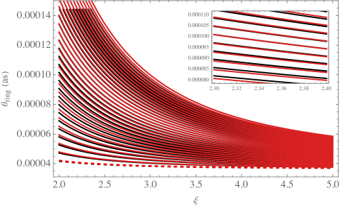
Figure 10: The profile of the Einstein ring’s radius in arcseconds, plotted for M87* (black curves) and Sgr A* (red curves). The plots are generated for $\alpha=0.1$, $\mathcal{k}=0.4$, $q=0.1$, and $\rho_{0}=1$. The observer’s location is considered to be $r_{\mathbb{O}}=D_{\mathrm{R}}$, and for simplicity, it is assumed that $D_{\mathrm{R}}=D_{\mathrm{S}}$ for both cases. The plots cover a range of the $\mathcal{B}$-parameter within the domain $\mathcal{B}\in(0,0.03)$, with increments of $0.001$. The dashed curves correspond to the Schwarzschild black hole for both cases.

Comparing with the diagram in Fig. 8(a), and based on the assumed distances for the source and receiver in Fig. 10, the angular radius of the Einstein ring is proportional to half of the deflection angle for each considered black hole. The profiles in the figure show that an increase in the $\mathcal{B}$-parameter leads to a larger angular radius of the ring. Despite the significant distance difference between M87* and Sgr A*, the variation in the ring’s angular radius between these two black holes is minimal. However, for a given impact parameter, an increase in the $\mathcal{B}$-parameter results in a larger angular radius for M87* compared to Sgr A*, which is more evident for smaller impact parameters as highlighted in the magnified segment of the diagram. This effect is attributed to the cosmological term in the GCJDF black hole, which becomes more prominent at larger distances. According to the results in Fig. 10, for large impact parameters, we can approximate $\theta_{\mathrm{ring}}^{\mathrm{Sch}}\approx 36.3\,\mathrm{\mu as}$, while $\theta_{\mathrm{ring}}^{\mathrm{GCJDF}}\approx 37.6284\,\mathrm{\mu as}$ for M87* and $\theta_{\mathrm{ring}}^{\mathrm{GCJDF}}\approx 37.6261\,\mathrm{\mu as}$ for Sgr A* with $\mathcal{B}=0.03$. These values fall within the detection capabilities of modern astronomical detectors. For instance, the EHT has an angular resolution of approximately $20\,\mathrm{\mu as}$ at 345 GHz [135]. Additionally, the Gaia space observatory can resolve around $7$-$20\,\mathrm{\mu as}$ [136]. It is noteworthy that the impact of the dark fluid becomes particularly evident for sources near the black hole, where the discrepancy between the ring’s radius of the GCJDF black hole and the Schwarzschild black hole is more noticeable. Consequently, Einstein rings are more detectable for more distant black holes when the light sources are positioned closer to them.

VI Summary and conclusions

In this paper, we investigated the optical properties of a static spherically symmetric black hole within the context of an anisotropic generalized Chaplygin-like gas. We began by reviewing the characteristics of the CG and its generalized counterpart (GCG), incorporating anisotropic properties through Jacobi elliptic functions, resulting in the GCJG model. We demonstrated that the EoS for the GCJG depends on the modulus of the elliptic function, the factor $\alpha$, and the parameter $\mathcal{B}$, which measures the prominence of the gas. Assuming this gas as the medium surrounding a static spherically symmetric black hole, termed the GCJDF, we derived a specific density profile aligned with the anisotropic energy-momentum tensor. Upon solving the Einstein equations for this black hole spacetime, we identified a radial-dependent cosmological term within the metric function, reducing to the Schwarzschild metric when $\mathcal{B}=0$. The analysis of energy conditions revealed that while the DEC is violated outside the Schwarzschild radius, the SEC is satisfied, highlighting the inflationary nature of the fluid. We explored light propagation in this spacetime by employing the Lagrangian framework for null geodesics in static spherically symmetric spacetimes, leading to the effective potential and the shadow parametrization of the black hole. Due to the non-asymptotic flatness of the black hole, we used a finite distance method to calculate the celestial coordinates and the shadow radius. Additionally, the energy emission rate and the deflection angle of light rays using the GBT were computed. Our findings indicate that decreasing anisotropy in the dark fluid results in larger shadow radii, with the Schwarzschild black hole providing the lower limit for shadow size and deflection angle, and the upper limit for evaporation rate. While the dark fluid enhances gravitational lensing, its anisotropy increases lensing efficacy as more light rays are deflected, with fewer being captured by the black hole. Comparing our results with the EHT observations of M87* and Sgr A*, we found that optimal parameter domains are $0<\alpha\lesssim 0.1$ and $0\leq\mathcal{B}\lesssim 0.03$. Finally, we analyzed the sizes of Einstein rings for both black holes, concluding that for M87*, the ring size becomes more prominent with increasing $\mathcal{B}$ due to the dominance of the cosmological term at larger distances. Our investigation into the optical properties of a black hole associated with a dark field can provide insights into the interplay between dark fluid anisotropy and light deflection, while constraints on the spacetime parameters validated by comparisons with the EHT observations, can help us in further explorations. Future work should aim to refine these models and extend the analysis to rotating black holes and other complex systems. These findings not only enhance our theoretical understanding but also pave the way for more precise astrophysical observations in the near future.

Appendix A Derivation of the density profile in Eq. (14)

The Einstein field equations (12) and (13) can be recast as

$$\frac{f}{r^{2}}+\frac{f^{\prime}}{r}-\frac{1}{r^{2}}=-\rho,$$ (81)

$$\frac{f^{\prime}}{r}+\frac{f^{\prime\prime}}{2}=p_{t}(\rho),$$ (82)

where the expression for $p_{t}$ has been given in Eq. (7). Differentiating Eq. (81) provides

$$-\frac{2f}{r^{3}}+\frac{f^{\prime\prime}}{r}+\frac{2}{r^{3}}=-\rho^{\prime}.$$ (83)

On the other hand, from Eq. (82) we have

$$\frac{f^{\prime\prime}}{r}=\frac{2}{r}\left[p_{t}(\rho)-\frac{f^{\prime}}{r}\right].$$ (84)

Employing Eqs. (83) and (84), we get

$$-\rho^{\prime}=\frac{2}{r}\underbrace{\left[\frac{1}{r^{2}}-\frac{f}{r^{2}}-\frac{f^{\prime}}{r}\right]}_{=\rho,\,\mathrm{from\,Eq.\,\eqref{eq:A1}}}+\frac{2p_{t}(\rho)}{r}=\frac{2}{r}\mathcal{F}(\rho),$$ (85)

in which $\mathcal{F}(\rho)=\rho+p_{t}(\rho)$, and by means of Eq. (7), we have

$$\mathcal{F}(\rho)=\frac{3}{2\rho^{\alpha}}\left[-B\mathcal{k}-(2\mathcal{k}^{\prime}-1)\rho^{\alpha+1}+\frac{\mathcal{k}^{\prime}}{B}\rho^{2(\alpha+1)}\right].$$ (86)

This way, Eq. (85) leads to the following differential equation:

$$-2\frac{\mathrm{d}r}{r}=\frac{\mathrm{d}\rho}{\mathcal{F}(\rho)}.$$ (87)

To solve the above equation, let us propose the change of the variable $X\doteq\rho^{\alpha+1}$. Accordingly, the differential equation changes to

$$\frac{2}{3(\alpha+1)}\,\frac{\mathrm{d}X}{-B\mathcal{k}-(2\mathcal{k}^{\prime}-1)X+\frac{\mathcal{k}^{\prime}}{B}X^{2}}=-2\frac{\mathrm{d}r}{r}.$$ (88)

Assuming $B<0$, one needs to consider the absolute value of this parameter, and Eq. (88) reshapes to

$$\frac{2}{3(\alpha+1)}\,\frac{\mathrm{d}X}{|B|\mathcal{k}-(1-2\mathcal{k})X-\frac{\mathcal{k}^{\prime}}{|B|}X^{2}}=-2\frac{\mathrm{d}r}{r}.$$ (89)

When $0<k<1$, one can integrate both sides of Eq. (89), which yields

$$\frac{2}{3(\alpha+1)}\ln\left(\frac{\mathcal{k}^{\prime}[X+|B|\,]}{|B|\mathcal{k}-\mathcal{k}^{\prime}X}\right) = -2\ln{r}+\frac{2}{3(\alpha+1)}\ln{q^{2}}$$

$$\Longrightarrow\ln\left(\frac{\mathcal{k}^{\prime}[X+|B|\,]}{|B|\mathcal{k}-\mathcal{k}^{\prime}X}\right) = \ln{\left(\frac{q^{2}}{r^{3(\alpha+1)}}\right)}$$

$$\Longrightarrow\frac{\mathcal{k}^{\prime}\left(X+|B|\right)}{|B|\mathcal{k}-\mathcal{k}^{\prime}X} = \frac{q^{2}}{r^{3(\alpha+1)}}$$

$$\stackrel{{\scriptstyle\mathrm{change\,of\,variable}}}{{\xRightarrow{\hskip 56.9055pt}}}\frac{\mathcal{k}^{\prime}\left(\rho^{\alpha+1}+|B|\right)}{|B|\mathcal{k}-\mathcal{k}^{\prime}\rho^{\alpha+1}} = \frac{q^{2}}{r^{3(\alpha+1)}}\doteq y(r).$$ (90)

By defining $B=-\rho_{0}^{\alpha+1}\mathcal{B}$ with $(\rho_{0},\mathcal{B})>0$ to ensure the condition $B<0$, Eq. (90) yields

$$\frac{\mathcal{k}^{\prime}\left({\rho}/{\rho_{0}}\right)^{\alpha+1}\left(1+\mathcal{B}\right)}{\mathcal{k}^{\prime}\left({\rho}/{\rho_{0}}\right)^{\alpha+1}\left(1-\mathcal{k}\mathcal{B}\right)}=y(r).$$ (91)

This will result in the solution (14).

References

- [1] V. C. Rubin, W. K. Ford, Jr., and N. Thonnard, “Rotational properties of 21 sc galaxies with a large range of luminosities and radii, from ngc 4605 /r = 4kpc/ to ugc 2885 /r = 122 kpc/,” Astrophys. J, vol. 238, pp. 471–487, jun 1980.
- [2] R. Massey, T. Kitching, and J. Richard, “The dark matter of gravitational lensing,” Rept. Prog. Phys., vol. 73, p. 086901, 2010.
- [3] K. Bolejko, C. Clarkson, R. Maartens, D. Bacon, N. Meures, and E. Beynon, “Antilensing: The bright side of voids,” Phys. Rev. Lett., vol. 110, p. 021302, Jan 2013.
- [4] A. G. Riess et al., “Observational evidence from supernovae for an accelerating universe and a cosmological constant,” Astron. J., vol. 116, pp. 1009–1038, 1998.
- [5] S. Perlmutter et al., “Measurements of omega and lambda from 42 high redshift supernovae,” Astrophys. J., vol. 517, pp. 565–586, 1999.
- [6] P. Astier, “The expansion of the universe observed with supernovae,” arXiv e-prints, p. arXiv:1211.2590, Nov 2012.
- [7] C. L. Bennett, A. Kogut, G. Hinshaw, A. J. Banday, E. L. Wright, K. M. Gorski, D. T. Wilkinson, R. Weiss, G. F. Smoot, S. S. Meyer, and et al., “Cosmic temperature fluctuations from two years of cobe differential microwave radiometers observations,” The Astrophysical Journal, vol. 436, p. 423, Dec 1994.
- [8] A. Kamenshchik, U. Moschella, and V. Pasquier, “An alternative to quintessence,” Physics Letters B, vol. 511, p. 265–268, July 2001.
- [9] J. Fabris, S. Gonçalves, and P. de Souza, “Letter: Density perturbations in a universe dominated by the chaplygin gas,” General Relativity and Gravitation, vol. 34, p. 53–63, Jan. 2002.
- [10] M. C. Bento, O. Bertolami, and A. A. Sen, “Generalized chaplygin gas, accelerated expansion, and dark-energy-matter unification,” Physical Review D, vol. 66, Aug. 2002.
- [11] K. Akiyama et al., “First M87 Event Horizon Telescope Results. I. The Shadow of the Supermassive Black Hole,” Astrophys. J., vol. 875, no. 1, p. L1, 2019.
- [12] K. Akiyama et al., “First Sagittarius A∗ Event Horizon Telescope results. I. The shadow of the supermassive black hole in the center of the Milky Way.,” Astrophys. J. Lett., vol. 930, no. 2, p. L12, 2022.
- [13] A. Pizzella, E. M. Corsini, J. C. Vega Beltrán, L. Coccato, and F. Bertola, “Supermassive black holes and dark matter halos,” Memorie della Societa Astronomica Italiana, vol. 74, p. 504, Jan. 2003. ADS Bibcode: 2003MmSAI..74..504P.
- [14] L. Ferrarese, “Beyond the Bulge: A Fundamental Relation between Supermassive Black Holes and Dark Matter Halos,” The Astrophysical Journal, vol. 578, pp. 90–97, Oct. 2002.
- [15] B. M. Sabra, M. A. Akl, and G. Chahine, “The black hole-dark matter halo connection,” Proceedings of the International Astronomical Union, vol. 3, pp. 257–258, July 2007.
- [16] M. Volonteri, P. Natarajan, and K. Gültekin, “How important is the dark matter halo for black hole growth?,” The Astrophysical Journal, vol. 737, p. 50, Aug. 2011.
- [17] Z. Xu, X. Hou, X. Gong, and J. Wang, “Black hole space-time in dark matter halo,” Journal of Cosmology and Astroparticle Physics, vol. 2018, pp. 038–038, sep 2018.
- [18] K. Jusufi, M. Jamil, and T. Zhu, “Shadows of Sgr A* black hole surrounded by superfluid dark matter halo,” The European Physical Journal C, vol. 80, p. 354, May 2020.
- [19] Z. Xu, X. Gong, and S.-N. Zhang, “Black hole immersed dark matter halo,” Physical Review D, vol. 101, p. 024029, Jan. 2020.
- [20] M. R. S. Hawkins, “The signature of primordial black holes in the dark matter halos of galaxies,” Astronomy & Astrophysics, vol. 633, p. A107, Jan. 2020.
- [21] P. Villanueva-Domingo, O. Mena, and S. Palomares-Ruiz, “A Brief Review on Primordial Black Holes as Dark Matter,” Frontiers in Astronomy and Space Sciences, vol. 8, p. 681084, May 2021.
- [22] A. Das, A. Saha, and S. Gangopadhyay, “Investigation of circular geodesics in a rotating charged black hole in the presence of perfect fluid dark matter,” Classical and Quantum Gravity, vol. 38, p. 065015, feb 2021.
- [23] D. Liu, Y. Yang, S. Wu, Y. Xing, Z. Xu, and Z.-W. Long, “Ringing of a black hole in a dark matter halo,” Physical Review D, vol. 104, p. 104042, Nov. 2021.
- [24] J. Liu, S. Chen, and J. Jing, “Tidal effects of a dark matter halo around a galactic black hole*,” Chinese Physics C, vol. 46, p. 105104, Oct. 2022.
- [25] R. C. Pantig and A. Övgün, “Black Hole in Quantum Wave Dark Matter,” Fortschritte der Physik, vol. 71, p. 2200164, Jan. 2023.
- [26] S. V. Xavier, H. C. Lima Junior, and L. C. Crispino, “Shadows of black holes with dark matter halo,” Physical Review D, vol. 107, p. 064040, Mar. 2023.
- [27] C. Stelea, M.-A. Dariescu, and C. Dariescu, “Charged black holes with dark halos,” Physics Letters B, vol. 847, p. 138275, Dec. 2023.
- [28] A. Övgün, L. J. F. Sese, and R. C. Pantig, “Constraints via the Event Horizon Telescope for Black Hole Solutions with Dark Matter under the Generalized Uncertainty Principle Minimal Length Scale Effect,” Annalen der Physik, vol. 536, p. 2300390, Apr. 2024.
- [29] Y. Yang, D. Liu, A. Övgün, G. Lambiase, and Z.-W. Long, “Black hole surrounded by the pseudo-isothermal dark matter halo,” The European Physical Journal C, vol. 84, p. 63, Jan. 2024.
- [30] D. Liu, Y. Yang, Z. Xu, and Z.-W. Long, “Modeling the black holes surrounded by a dark matter halo in the galactic center of M87,” The European Physical Journal C, vol. 84, p. 136, Feb. 2024.
- [31] S. Wu, B. Wang, Z. Long, and H. Chen, “Rotating black holes surrounded by a dark matter halo in the galactic center of M87 and Sgr A*,” Physics of the Dark Universe, vol. 44, p. 101455, May 2024.
- [32] V. V. Kiselev, “Quintessence and black holes,” Classical and Quantum Gravity, vol. 20, pp. 1187–1197, Mar. 2003.
- [33] J. A. Jimenez Madrid and P. F. Gonzalez-Diaz, “Evolution of a kerr-newman black hole in a dark energy universe,” Grav. Cosmol., vol. 14, pp. 213–225, 2008.
- [34] H. Maeda, T. Harada, and B. J. Carr, “Self-similar cosmological solutions with dark energy. II. Black holes, naked singularities, and wormholes,” Physical Review D, vol. 77, p. 024023, Jan. 2008.
- [35] M. Jamil, “Evolution of a Schwarzschild black hole in phantom-like Chaplygin gas cosmologies,” Eur. Phys. J. C, vol. 62, pp. 609–614, 2009.
- [36] L. Mersini-Houghton and A. Kelleher, “Investigating Dark Energy with Black Hole Binaries,” Nuclear Physics B - Proceedings Supplements, vol. 194, pp. 272–277, Oct. 2009.
- [37] P. Martín-Moruno, A.-E. L. Marrakchi, S. Robles-Pérez, and P. F. González-Díaz, “Dark energy accretion onto black holes in a cosmic scenario,” General Relativity and Gravitation, vol. 41, pp. 2797–2811, Dec. 2009.
- [38] S. Cheng-Yi, “Dark Energy Accretion onto a Black Hole in an Expanding Universe,” Communications in Theoretical Physics, vol. 52, pp. 441–444, Sept. 2009.
- [39] S. Fernando, “NARIAI BLACK HOLES WITH QUINTESSENCE,” Modern Physics Letters A, vol. 28, p. 1350189, Dec. 2013.
- [40] E. O. Babichev, V. I. Dokuchaev, and Y. N. Eroshenko, “Black holes in the presence of dark energy,” Physics-Uspekhi, vol. 56, pp. 1155–1175, Dec. 2013.
- [41] S. G. Ghosh, “Rotating black hole and quintessence,” The European Physical Journal C, vol. 76, p. 222, Apr. 2016.
- [42] J. De Oliveira and R. Fontana, “Three-dimensional black holes with quintessence,” Physical Review D, vol. 98, p. 044005, Aug. 2018.
- [43] M. Fathi, M. Olivares, and J. R. Villanueva, “Study of null and time-like geodesics in the exterior of a Schwarzschild black hole with quintessence and cloud of strings,” The European Physical Journal C, vol. 82, p. 629, July 2022.
- [44] M. Rogatko, “Dark photon–dark energy stationary axisymmetric black holes,” Physical Review D, vol. 109, p. 104030, May 2024.
- [45] A. Singh, A. Ghosh, and C. Bhamidipati, “Thermodynamic Curvature of AdS Black Holes with Dark Energy,” Frontiers in Physics, vol. 9, p. 631471, Mar. 2021.
- [46] S. Hui, B. Mu, and P. Wang, “Echoes from charged black holes influenced by quintessence,” Physics of the Dark Universe, vol. 43, p. 101396, Feb. 2024.
- [47] N. Bilić, G. Tupper, and R. Viollier, “Unification of dark matter and dark energy: the inhomogeneous chaplygin gas,” Physics Letters B, vol. 535, p. 17–21, May 2002.
- [48] J. R. Villanueva, “The generalized Chaplygin-Jacobi gas,” JCAP, vol. 07, p. 045, 2015.
- [49] P. F. Byrd and M. D. Friedman, Handbook of Elliptic Integrals for Engineers and Scientists. Berlin, Heidelberg: Springer Berlin Heidelberg, 1971.
- [50] I. Semiz, “All ”static” spherically symmetric perfect fluid solutions of einstein’s equations with constant equation of state parameter and finite polynomial ”mass function”,” Reviews in Mathematical Physics, vol. 23, no. 08, pp. 865–882, 2011.
- [51] V. V. Kiselev, “Quintessence and black holes,” Classical and Quantum Gravity, vol. 20, pp. 1187–1197, Mar. 2003.
- [52] K. Nozari, T. Azizi, and N. Alipour, “Observational constraints on Chaplygin cosmology in a braneworld scenario with induced gravity and curvature effect: Constraints on Chaplygin cosmology,” Monthly Notices of the Royal Astronomical Society, vol. 412, pp. 2125–2136, Apr. 2011.
- [53] H. B. Benaoum, “Modified Chaplygin Gas Cosmology,” Advances in High Energy Physics, vol. 2012, pp. 1–12, 2012.
- [54] N. Hulke, G. Singh, B. K. Bishi, and A. Singh, “Variable Chaplygin gas cosmologies in f(R, T) gravity with particle creation,” New Astronomy, vol. 77, p. 101357, May 2020.
- [55] S. Ray, S. K. Tripathy, R. Sengupta, B. Bal, and S. M. Rout, “Anisotropic Universes Sourced by Modified Chaplygin Gas,” Universe, vol. 9, p. 453, Oct. 2023.
- [56] U. Debnath, A. Banerjee, and S. Chakraborty, “Role of modified Chaplygin gas in accelerated universe,” Classical and Quantum Gravity, vol. 21, pp. 5609–5617, Dec. 2004.
- [57] M. K. Mak and T. Harko, “Chaplygin gas dominated anisotropic brane world cosmological models,” Phys. Rev. D, vol. 71, p. 104022, May 2005.
- [58] G. Raposo, P. Pani, M. Bezares, C. Palenzuela, and V. Cardoso, “Anisotropic stars as ultracompact objects in general relativity,” Phys. Rev. D, vol. 99, p. 104072, May 2019.
- [59] X.-Q. Li, H.-P. Yan, L.-L. Xing, and S.-W. Zhou, “Critical behavior of AdS black holes surrounded by dark fluid with Chaplygin-like equation of state,” Phys. Rev. D, vol. 107, no. 10, p. 104055, 2023.
- [60] D. Arora, M. Yasir, H. Chaudhary, F. Javed, G. Mustafa, X. Tiecheng, and F. Atamurotov, “Joule-Thomson expansion and tidal force effects of AdS black holes surrounded by Chaplygin dark fluid,” arXiv e-prints, p. arXiv:2312.16224, Dec. 2023.
- [61] G. Mustafa, S. K. Maurya, A. Ditta, S. Ray, and F. Atamurotov, “Circular orbits and accretion disk around AdS black holes surrounded by dark fluid with Chaplygin-like equation of state,” arXiv e-prints, p. arXiv:2311.13839, Nov. 2023.
- [62] M. Visser and C. Barceló, “Energy conditions and their cosmological implications,” in COSMO-99, (ICTP, Trieste, Italy), pp. 98–112, World Scientific, Sept. 2000.
- [63] O. Zaslavskii, “Regular black holes and energy conditions,” Physics Letters B, vol. 688, pp. 278–280, May 2010.
- [64] J. Neves and A. Saa, “Regular rotating black holes and the weak energy condition,” Physics Letters B, vol. 734, pp. 44–48, June 2014.
- [65] E.-A. Kontou and K. Sanders, “Energy conditions in general relativity and quantum field theory,” Classical and Quantum Gravity, vol. 37, p. 193001, Oct. 2020.
- [66] S. Capozziello, F. S. Lobo, and J. P. Mimoso, “Energy conditions in modified gravity,” Physics Letters B, vol. 730, pp. 280–283, Mar. 2014.
- [67] J. D. Barrow, “String-driven inflationary and deflationary cosmological models,” Nuclear Physics B, vol. 310, no. 3, pp. 743–763, 1988.
- [68] I. Klaoudatou, The nature of cosmological singularities in isotropic universes and braneworlds. PhD thesis, -, June 2008.
- [69] J. D. Barrow, “Cosmic no-hair theorems and inflation,” Physics Letters B, vol. 187, no. 1, pp. 12–16, 1987.
- [70] M. Giovannini, “Relic gravitons, dominant energy condition, and bulk viscous stresses,” Physical Review D, vol. 59, p. 121301, May 1999.
- [71] R. Caldwell, “A phantom menace? Cosmological consequences of a dark energy component with super-negative equation of state,” Physics Letters B, vol. 545, pp. 23–29, Oct. 2002.
- [72] V. Lasukov, “Violation of the Dominant Energy Condition in Geometrodynamics,” Symmetry, vol. 12, p. 400, Mar. 2020.
- [73] S. Conboy and K. Lake, “Smooth transitions from the Schwarzschild vacuum to de Sitter space,” Physical Review D, vol. 71, p. 124017, June 2005.
- [74] M. J. Schlosser, “Multiple Hypergeometric Series: Appell Series and Beyond,” in Computer Algebra in Quantum Field Theory (C. Schneider and J. Blümlein, eds.), pp. 305–324, Vienna: Springer Vienna, 2013.
- [75] E. Gallo, C. Kozameh, T. Mädler, O. M. Moreschi, and A. Perez, “Spherically symmetric black holes and affine-null metric formulation of einstein’s equations,” Phys. Rev. D, vol. 104, p. 084048, Oct 2021.
- [76] A. B. Nielsen and J. H. Yoon, “Dynamical surface gravity,” Classical and Quantum Gravity, vol. 25, p. 085010, Apr. 2008.
- [77] M. Pielahn, G. Kunstatter, and A. B. Nielsen, “Dynamical surface gravity in spherically symmetric black hole formation,” Phys. Rev. D, vol. 84, p. 104008, Nov 2011.
- [78] S. Chandrasekhar, The mathematical theory of black holes. Oxford classic texts in the physical sciences, Oxford: Oxford Univ. Press, 2002.
- [79] B. Carter, “Global structure of the kerr family of gravitational fields,” Phys. Rev., vol. 174, pp. 1559–1571, Oct 1968.
- [80] J. Bardeen, “Timelike and null geodesics in the Kerr metric,” in Les Houches Summer School of Theoretical Physics: Black Holes, pp. 215–240, 1973.
- [81] J. L. Synge, “The Escape of Photons from Gravitationally Intense Stars,” Mon. Not. Roy. Astron. Soc., vol. 131, pp. 463–466, 02 1966.
- [82] C. T. Cunningham and J. M. Bardeen, “The Optical Appearance of a Star Orbiting an Extreme Kerr Black Hole,” Astrophys. J. Letters, vol. 173, p. L137, May 1972.
- [83] J. M. Bardeen, W. H. Press, and S. A. Teukolsky, “Rotating Black Holes: Locally Nonrotating Frames, Energy Extraction, and Scalar Synchrotron Radiation,” Astrophys. J, vol. 178, pp. 347–370, Dec. 1972.
- [84] J. P. Luminet, “Image of a spherical black hole with thin accretion disk.,” A&A, vol. 75, pp. 228–235, May 1979.
- [85] J. M. Bardeen, W. H. Press, and S. A. Teukolsky, “Rotating Black Holes: Locally Nonrotating Frames, Energy Extraction, and Scalar Synchrotron Radiation,” Astrophys. J. , vol. 178, pp. 347–370, Dec. 1972.
- [86] I. Bray, “Kerr black hole as a gravitational lens,” Phys. Rev., vol. D34, pp. 367–372, Jul 1986.
- [87] S. E. Vázquez and E. P. Esteban, “Strong-field gravitational lensing by a Kerr black hole,” Nuovo Cimento B Serie, vol. 119, p. 489, May 2004.
- [88] A. Grenzebach, V. Perlick, and C. Lämmerzahl, “Photon regions and shadows of kerr-newman-nut black holes with a cosmological constant,” Phys. Rev., vol. D89, p. 124004, Jun 2014.
- [89] A. Grenzebach, The Shadow of Black Holes, pp. 55–79. Cham: Springer International Publishing, 2016.
- [90] V. Perlick, O. Y. Tsupko, and G. S. Bisnovatyi-Kogan, “Black hole shadow in an expanding universe with a cosmological constant,” Phys. Rev., vol. D97, p. 104062, May 2018.
- [91] G. S. Bisnovatyi-Kogan and O. Y. Tsupko, “Shadow of a black hole at cosmological distances,” Phys. Rev., vol. D98, p. 084020, Oct 2018.
- [92] A. de Vries, “The apparent shape of a rotating charged black hole, closed photon orbits and the bifurcation set a 4,” Classical and Quantum Gravity, vol. 17, pp. 123–144, dec 1999.
- [93] Z.-Q. Shen, K. Y. Lo, M.-C. Liang, P. T. P. Ho, and J.-H. Zhao, “A size of 1 au for the radio source sgr a* at the centre of the milky way,” Nature, vol. 438, pp. 62–64, Nov 2005.
- [94] L. Amarilla, E. F. Eiroa, and G. Giribet, “Null geodesics and shadow of a rotating black hole in extended chern-simons modified gravity,” Phys. Rev., vol. D81, p. 124045, Jun 2010.
- [95] L. Amarilla and E. F. Eiroa, “Shadow of a rotating braneworld black hole,” Phys. Rev., vol. D85, p. 064019, Mar 2012.
- [96] A. Yumoto, D. Nitta, T. Chiba, and N. Sugiyama, “Shadows of multi-black holes: Analytic exploration,” Phys. Rev., vol. D86, p. 103001, Nov 2012.
- [97] L. Amarilla and E. F. Eiroa, “Shadow of a kaluza-klein rotating dilaton black hole,” Phys. Rev., vol. D87, p. 044057, Feb 2013.
- [98] F. Atamurotov, A. Abdujabbarov, and B. Ahmedov, “Shadow of rotating non-kerr black hole,” Phys. Rev., vol. D88, p. 064004, Sep 2013.
- [99] A. A. Abdujabbarov, L. Rezzolla, and B. J. Ahmedov, “A coordinate-independent characterization of a black hole shadow,” Monthly Notices of the Royal Astronomical Society, vol. 454, pp. 2423–2435, 10 2015.
- [100] A. Abdujabbarov, M. Amir, B. Ahmedov, and S. G. Ghosh, “Shadow of rotating regular black holes,” Phys. Rev., vol. D93, p. 104004, May 2016.
- [101] M. Amir, B. P. Singh, and S. G. Ghosh, “Shadows of rotating five-dimensional charged emcs black holes,” The European Physical Journal C, vol. 78, p. 399, May 2018.
- [102] N. Tsukamoto, “Black hole shadow in an asymptotically flat, stationary, and axisymmetric spacetime: The kerr-newman and rotating regular black holes,” Phys. Rev., vol. D97, p. 064021, Mar 2018.
- [103] P. V. P. Cunha and C. A. R. Herdeiro, “Shadows and strong gravitational lensing: a brief review,” Gen. Relativ. Gravit., vol. 50, p. 42, Mar 2018.
- [104] Y. Mizuno, Z. Younsi, C. M. Fromm, O. Porth, M. De Laurentis, H. Olivares, H. Falcke, M. Kramer, and L. Rezzolla, “The current ability to test theories of gravity with black hole shadows,” Nature Astronomy, vol. 2, pp. 585–590, Jul 2018.
- [105] A. K. Mishra, S. Chakraborty, and S. Sarkar, “Understanding photon sphere and black hole shadow in dynamically evolving spacetimes,” Phys. Rev., vol. D99, p. 104080, May 2019.
- [106] R. Kumar, A. Kumar, and S. G. Ghosh, “Testing rotating regular metrics as candidates for astrophysical black holes,” Astrophys. J., vol. 896, p. 89, jun 2020.
- [107] M. Zhang and M. Guo, “Can shadows reflect phase structures of black holes?,” Eur. Phys. J., vol. C80, p. 790, Aug 2020.
- [108] A. Belhaj, L. Chakhchi, H. El Moumni, J. Khalloufi, and K. Masmar, “Thermal image and phase transitions of charged ads black holes using shadow analysis,” Int. J. Mod. Phys. A, vol. 35, no. 27, p. 2050170, 2020.
- [109] M. Kramer, D. Backer, J. Cordes, T. Lazio, B. Stappers, and S. Johnston, “Strong-field tests of gravity using pulsars and black holes,” New Astronomy Reviews, vol. 48, no. 11, pp. 993 – 1002, 2004. Science with the Square Kilometre Array.
- [110] D. Psaltis, “Probes and tests of strong-field gravity with observations in the electromagnetic spectrum,” Living Reviews in Relativity, vol. 11, p. 9, Nov 2008.
- [111] T. Harko, Z. Kovács, and F. S. N. Lobo, “Testing hořava-lifshitz gravity using thin accretion disk properties,” Phys. Rev., vol. D80, p. 044021, Aug 2009.
- [112] D. Psaltis, F. Özel, C.-K. Chan, and D. P. Marrone, “A GENERAL RELATIVISTIC NULL HYPOTHESIS TEST WITH EVENT HORIZON TELESCOPE OBSERVATIONS OF THE BLACK HOLE SHADOW IN sgr a*,” Astrophys. J., vol. 814, p. 115, nov 2015.
- [113] T. Johannsen, A. E. Broderick, P. M. Plewa, S. Chatzopoulos, S. S. Doeleman, F. Eisenhauer, V. L. Fish, R. Genzel, O. Gerhard, and M. D. Johnson, “Testing general relativity with the shadow size of sgr ,” Phys. Rev. Lett., vol. 116, p. 031101, Jan 2016.
- [114] D. Psaltis, “Testing general relativity with the event horizon telescope,” Gen. Relativ. Gravit., vol. 51, p. 137, Oct 2019.
- [115] I. Dymnikova and K. Kraav, “Identification of a regular black hole by its shadow,” Universe, vol. 5, no. 7, 2019.
- [116] R. Kumar and S. G. Ghosh, “Black hole parameter estimation from its shadow,” Astrophys. J., vol. 892, p. 78, mar 2020.
- [117] A. Belhaj, M. Benali, A. El Balali, H. El Moumni, and S.-E. Ennadifi, “Deflection angle and shadow behaviors of quintessential black holes in arbitrary dimensions,” Classical and Quantum Gravity, vol. 37, p. 215004, Nov. 2020.
- [118] S.-W. Wei and Y.-X. Liu, “Observing the shadow of Einstein-Maxwell-Dilaton-Axion black hole,” Journal of Cosmology and Astroparticle Physics, vol. 2013, pp. 063–063, Nov. 2013.
- [119] Y. Décanini, A. Folacci, and B. Raffaelli, “Fine structure of high-energy absorption cross sections for black holes,” Classical and Quantum Gravity, vol. 28, p. 175021, Sept. 2011.
- [120] P.-C. Li, M. Guo, and B. Chen, “Shadow of a spinning black hole in an expanding universe,” Physical Review D, vol. 101, p. 084041, Apr. 2020.
- [121] K. S. Virbhadra and G. F. R. Ellis, “Schwarzschild black hole lensing,” Physical Review D, vol. 62, p. 084003, Sept. 2000.
- [122] K. S. Virbhadra and G. F. R. Ellis, “Gravitational lensing by naked singularities,” Physical Review D, vol. 65, p. 103004, May 2002.
- [123] K. S. Virbhadra and C. R. Keeton, “Time delay and magnification centroid due to gravitational lensing by black holes and naked singularities,” Physical Review D, vol. 77, p. 124014, June 2008.
- [124] K. S. Virbhadra, “Relativistic images of Schwarzschild black hole lensing,” Physical Review D, vol. 79, p. 083004, Apr. 2009.
- [125] K. Virbhadra, “Distortions of images of Schwarzschild lensing,” Physical Review D, vol. 106, p. 064038, Sept. 2022.
- [126] K. Virbhadra, “Conservation of distortion of gravitationally lensed images,” Physical Review D, vol. 109, p. 124004, June 2024.
- [127] K. S. Virbhadra, “Images Distortion Hypothesis,” Feb. 2024. arXiv:2402.17190 [astro-ph, physics:gr-qc].
- [128] G. W. Gibbons and M. C. Werner, “Applications of the Gauss–Bonnet theorem to gravitational lensing,” Classical and Quantum Gravity, vol. 25, p. 235009, Dec. 2008.
- [129] H. Arakida, “Light deflection and Gauss–Bonnet theorem: definition of total deflection angle and its applications,” General Relativity and Gravitation, vol. 50, p. 48, May 2018.
- [130] W. Klingenberg, A Course in Differential Geometry, vol. 51 of Graduate Texts in Mathematics. New York, NY: Springer New York, 1978.
- [131] K. Tapp, Differential Geometry of Curves and Surfaces. Undergraduate Texts in Mathematics, Cham: Springer International Publishing, 2016.
- [132] A. Ishihara, Y. Suzuki, T. Ono, T. Kitamura, and H. Asada, “Gravitational bending angle of light for finite distance and the gauss-bonnet theorem,” Phys. Rev. D, vol. 94, p. 084015, Oct 2016.
- [133] C. Bambi, K. Freese, S. Vagnozzi, and L. Visinelli, “Testing the rotational nature of the supermassive object M87* from the circularity and size of its first image,” Phys. Rev. D, vol. 100, no. 4, p. 044057, 2019.
- [134] V. Bozza, “Comparison of approximate gravitational lens equations and a proposal for an improved new one,” Phys. Rev. D, vol. 78, p. 103005, Nov 2008.
- [135] J.-Y. Kim et al., “Event Horizon Telescope imaging of the archetypal blazar 3C 279 at an extreme 20 microarcsecond resolution,” Astronomy & Astrophysics, vol. 640, p. A69, Aug. 2020.
- [136] L.-H. Liu and T. Prokopec, “Gravitational microlensing in Verlinde’s emergent gravity,” Physics Letters B, vol. 769, pp. 281–288, June 2017.