Anomaly Multi-classification in Industrial Scenarios: Transferring Few-shot Learning to a New Task

Abstract

In industrial scenarios, it is crucial not only to identify anomalous items but also to classify the type of anomaly. However, research on anomaly multi-classification remains largely unexplored. This paper proposes a novel and valuable research task called anomaly multi-classification. Given the challenges in applying few-shot learning to this task, due to limited training data and unique characteristics of anomaly images, we introduce a baseline model that combines RelationNet and PatchCore. We propose a data generation method that creates pseudo classes and a corresponding proxy task, aiming to bridge the gap in transferring few-shot learning to industrial scenarios. Furthermore, we utilize contrastive learning to improve the vanilla baseline, achieving much better performance than directly fine-tune a ResNet. Experiments conducted on MvTec AD and MvTec3D AD demonstrate that our approach shows superior performance in this novel task.

Keywords Anomaly Classification  $\cdot$ Few-shot Learning  $\cdot$ PatchCore

1 Introduction

In the realm of industrial production, anomaly detection plays a critical role, yet acquiring sufficient defective samples remains a formidable challenge. Various unsupervised anomaly detection methods have emerged. Among the various strategies, PatchCore[1] is a notable effective method, leveraging local image information to pinpoint anomalies. Its core concept involves segmenting the image into patches, extracting and modeling features for each patch, and comparing the features of each test sample’s patches with those of normal samples to achieve anomaly detection.

Moreover, the field has seen advancements in anomaly detection algorithms tailored for scenarios characterized by a scant number of normal samples, known as few-shot situations. Here, few-shot refers to situations with a small number of normal samples, such as WinCLIP[2]. It primarily leverages the powerful feature extraction capability of pre-trained CLIP to partition images into multiple windows, using textual prompts to achieve anomaly detection even with limited or zero normal samples. It is important to note, however, that this paper adopts a distinct interpretation of ‘few-shot’ compared to its application in WinCLIP. Few-shot in this paper means few-shot defect samples for multi-classification, rather than few-shot normal samples.

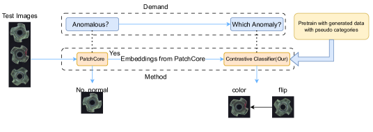
Figure 1: An simple illustration for our method

In practical industrial production, normal samples are usually easy to obtain, while defective samples are hard to acquire. Acknowledging this challenge, we propose a pragmatic task framework that begins with a substantial collection of normal samples, providing only a few samples of different categories of anomalies, the demand is to accurately classify new samples into the specific category of defects. This approach diverges from the conventional anomaly classification paradigm, which is predominantly concerned with the binary determination of defect presence and is essentially a binary classification problem. Our proposed task is a multi-classification problem built upon binary classification assumptions, leveraging the high accuracy of methods like PatchCore to detect all defect samples and then focusing on how to classify defect samples in a few-shot scenario.

Building upon the discussed concepts, the focus shifts to the domain of few-shot learning, a promising avenue for addressing these challenges. Concerning few-shot learning[3] from the general perspective. In the domain of few-shot image classification, datasets are typically split into training, validation, and test sets. However, the unique aspect of this learning paradigm is that the categories in these three subsets do not overlap. In few-shot learning, each sub-dataset consists of a query set and a support set, both containing data from the same categories, akin to the training and testing sets in traditional tasks.

Most research in this filed is at an early stage, with diverse methods including optimization-based MAML[4], graph network-based learning[5], and others. This paper focuses on some typical model-based methods such as Siamese Network [6], Matching Network[7], Prototypical Network[8], and RelationNet[9]. We will build a vanilla baseline based on RelationNet’s concept.

Now, the truth is that in industrial scenarios we only have a few defect samples, so that we lack a training dataset that contains different defect classes which do not overlap real defect categories. Thus we can not directly use model-based method in few-shot learning. Faced with this severe scenario, we have to consider few shot learning under the perspective of data generation, by such way, we can easily transfer other few-shot learning method into industrial scenarios, rather than developing new methods especially for industrial scenarios.

Consequently, we introduce a method that seamlessly integrates with anomaly detection processes, and we propose some data generation method to address the lack of defect samples for pretraining in the procedure of few-shot learning. As shown in Figure 1. Firstly we detect anomalous image by methods like PatchCore, then we feed the residual representations to a classification model, finally we know which anomaly the test image belong to.

In our endeavor to transpose the insights from few-shot learning research to the sphere of industrial anomaly classification, we have undertaken the following efforts:

• We establish a vanilla baseline based on the RelationNet network for a novel and valuable task called few-shot anomaly multi-classification.

• We propose a data generation method, and utilized them to pre-train the network on proxy tasks, confirming the effectiveness of data generation and proxy tasks in transferring few-shot learning to anomaly classification tasks, thus addressing the issue of lacking training sets while transferring few-shot learning methods into industrial data.

• By using residual representations extracted by PatchCore rather than raw image features, we enhance classification performance and making the vanilla baseline more suitable for industrial anomaly classification tasks.

• We propose some modifications to vanilla baseline inspired by contrastive learning, improving classification performance.

2 Related Work

2.1 Anomaly Detection

Feature-based methods dominate anomaly detection. SPADE[10] uses the KNN algorithm, leveraging a pre-trained CNN on ImageNet[11] for feature extraction, creating a normal instance database. It employs KNN for finding the K closest normal instances and uses feature pyramid matching for pixel-level detection. Similarly, PaDim[12] models feature distributions in image patches, while PatchCore[1] forms a core set from these patches, clustering normal features with KNN. CPR[13] accelerates matching with histogram similarity, and ReConPatch [14] enhances PatchCore with contrastive learning.

PRN[15] detects anomalies by calculating residual features and training a post-processing model, showcasing a hybrid learning approach.

These methods, focusing on binary classification, whose target is to locate the anomaly, differs from our multi-classification approach, whose task is to distinguish the anomaly after we locate the anomaly. A binary classification only need to recognize normal patterns, while multi-classification need to distinguish differences between anomalies. Although similar tasks such as anomaly clustering[16] emerge, they require ample defective samples.

2.2 Few-shot Learning

Few-shot learning spans knowledge transfer, including parameter sharing and meta-learning, and model-based approaches. Parameter sharing, covering fine-tuning to memory modules, includes Gong et al. ’s[17] Faster R-CNN adaptation for X-ray defect detection. Li, Junnan et al.[18] blend multi-task and few-shot learning, demonstrating the method’s versatility. Meta-learning applications, such as Lu et al. ’s[19] autoencoder training, follow a two-phase approach akin to MAML[4], showing promise for deployment scenarios. Key models like Siamese[6], Matching [7], Prototypical[8], and Relation Networks[9] have inspired enhancements for prototype identification, including Hou et al. ’s[20] cross-attention network. Graph learning, merging with metric learning, introduces novel few-shot learning approaches, exemplified by DPGN[5], integrating graph-based learning theory.

However, reliance on extensive pre-training datasets in few-shot learning poses challenges in data-scarce industrial scenarios, so that we can not directly transfer a few-shot learning method into industrial scenarios.

3 Method

3.1 Overview

In general, our method consists of three modules dedicated to transferring few-shot learning to anomaly multi-classification. First of all, we propose to pretrain with generated data to enhance the performance of our model. The data generation method is shown in Figure 4. Then we utilize the classic anomaly detection method PatchCore to get the nearest representations of input features, and then we get the residual representations, which can enhance the representation of abnormal areas in anomaly images. As shown in Figure 3. Finally we proposed a vanilla baseline for few-shot learning in anomaly multi-classification based on RelationNet and leverage contrastive learning to improve the vanilla baseline. As shown in Figure 3 and Figure 5.

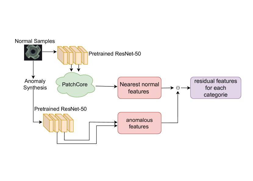
Figure 2: Residual Features Extraction

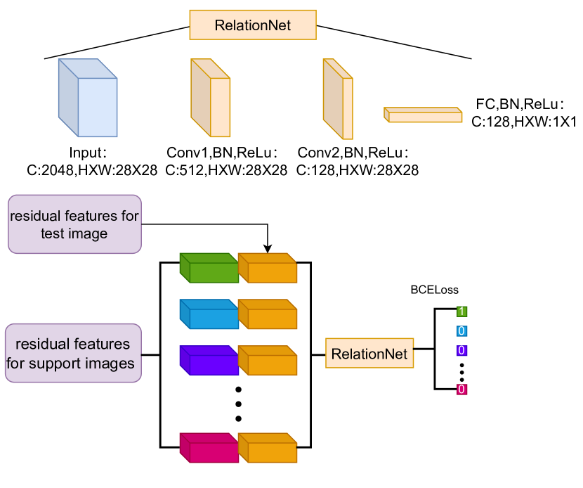
Figure 3: Vanilla Baseline Architecture

3.2 Revisiting the Features Extraction of PatchCore

This section follows the setting of PatchCore[1]. Assuming $\mathcal{X}$ is the set of normal samples, where the $i$-th sample $X_{i}\in\mathcal{X}$ is input into a pre-trained model such as ResNet-50[21]. From the $j$-th layer of the model’s output, denoted as $\mathcal{F}_{ij}$, we obtain a feature map. The depth of the feature map tensor $\mathcal{F}_{ij}$ is $c^{j}$, with height $h^{j}$ and width $w^{j}$, i.e., $\mathcal{F}_{ij}\in\mathbb{R}^{c_{j}\times h_{j}\times w_{j}}$. We extract features from the second and third layers, i.e., for each $X_{i}$, we extract $\mathcal{F}_{i2}\in\mathbb{R}^{c_{2}\times h_{2}\times w_{2}}$ and $\mathcal{F}_{i3}\in\mathbb{R}^{c_{3}\times h_{3}\times w_{3}}$. Then we patch each position for every sample $X_{i}$, resulting in feature dimensions of $(w_{2}h_{2},c_{2},3,3)$ and $(w_{3}h_{3},c_{3},3,3)$, respectively. For the features extracted from layer 3, they are upsampled to $(w_{2}h_{2},c_{3},3,3)$, then both sets of features undergo adaptive average pooling along the last three dimensions to $c_{3}$, resulting in features of dimensions $(w_{2}h_{2},c_{3})$ for each. Subsequently, these features are concatenated to obtain $(w_{2}h_{2},2,c_{3})$, and they are further aggregated(averaged) to obtain $(w_{2}h_{2},c_{3})$. For the features of normal samples, all sample features are aggregated into a memory bank $\mathcal{M}$, described by feature dimensions of $(N*w_{2}h_{2},c_{3})$, where $N$ denotes the number of normal samples, then memory bank downsampled to $(N_{d},c_{3})$, where $N_{d}$ denotes the number of downsampled features. In detail, we define a parameter $p$, where $N_{d}=N/p$. The downsampled features are sampled from $\mathcal{M}$, and are selected following the coreset subsampling[1]in PatchCore. For the features of abnormal or test samples, each image can be described as $A_{i}(w_{2}h_{2},c_{3})\in\mathcal{A}$, with $w_{2}h_{2}$ as feature numbers, which $\mathcal{A}$ denotes the set of test samples.

3.3 Vanilla Baseline

Inspired by RelationNet, we propose a vanilla baseline as shown in the Figure 3. In contrast to the original RelationNet, the main difference lies in that we use features extracted in the previous step rather than input images as the input, and then we design a multi-layer convolutional network. Additionally, we modify the original loss function from MSELoss to BCELoss(Equation 1) and weight the loss to address the imbalance between positive and negative samples. The reason is that it can performs better. Specifically, for the loss of positive sample categories (where features from the support set and query set belong to the same category), we assign a weight of $w=class\_number-1$.

$$L=-\frac{1}{N}\sum_{i=1}^{N}\left[w\cdot y_{i}\cdot\log(\hat{y}_{i})+(1-y_{i})\cdot\log(1-\hat{y}_{i})\right]$$ (1)

where $N$ denotes sample number, $y_{i}$ denotes the label of the sample, $\hat{y}_{i}$ denotes the prediction of the model

3.4 Residual Representation

To further leverage the characteristics of anomaly classification tasks, we propose a enhencement module for the original PatchCore that utilizes residual features. That is, for the features extracted as described in Subsection 3.2, let the features extracted from the input anomalous images be denoted as $A_{i}(w_{2}h_{2},c_{3})$. For any vector whose dimension is $c_{3}$, we search for the nearest neighbor $M(c_{3},)$ in the memory bank $\mathcal{M}$ and then compute the difference as follows:

$$D_{i}=A_{i}-M_{j}\quad where\quad j=\underset{M_{j}\in\mathcal{M}}{\text{argmin}}\|A_{i}-M_{j}\|$$ (2)

As a result, the input to the vanilla baseline will be residual features, rather than raw features.

3.5 Data Generation

Now, let’s review the typical settings of few-shot learning. The categories of items in the training set, as well as those in the testing and validation sets, do not overlap. This condition cannot be met for industrial data because defects of various categories are even scarcer resources and all categories of real defect should be in test set. Therefore, this paper proposes to artificially generate defect images with fabricated categories. A training set is created based on these fabricated defect images, where models can quickly transfer from the defined fabricated categories to real defect categories.

In other words, we define a proxy task by allowing the model to undergo initial classification training on the generated dataset with defined pseudo categories. Then, further fine-tuning training is conducted on few-shot real defect samples. Particularly, in a one-shot scenario where there is insufficient data for fine-tuning, the model trained on the generated dataset can directly classify, yielding satisfactory results in some specific item categories.

We define a data generation method, which is inspired by DRAEM[22], where we also use the DTD[23] dataset. This dataset defines 47 different textures. As shown in Figure 4. Firstly, segmentation methods are employed to obtain foreground-background segmentation masks not present in the original dataset. Backgrounds in industrial images are typically simple, so we employ traditional algorithms such as GrabCut[24] or flood fill algorithm. Initial seed points are chosen at the perimeter of images, allowing for straightforward extraction of foreground masks. Next, we randomly generate a Poisson noise image and perform threshold segmentation on it to obtain a mask. We then merge this mask with the original image, taking the intersection, to obtain a mask generated solely by Poisson noise on the foreground of the image, denoted as $M_{a}$. We then merge the texture image with $M_{a}$, taking the intersection, denoted as $M_{a}\odot A$. Finally, the resulting image is merged with the original image at a certain ratio $\beta$ to obtain the final fabricated defect image $R$. At last we define the category of the fabricated defect image as a category of the texture image. Note that this is not the same as DRAEM, as we remove any augmentation on the texture picture, we should keep the generation method naive to preserve the original texture.

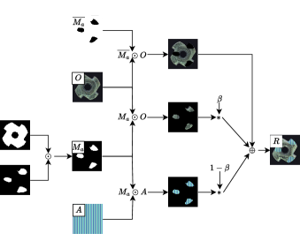
Figure 4: Data Generation Process

3.6 Contrastive Classifier

Inspired by the success of contrastive learning methods such as SimCLR[25] and MOCO[26], we propose further modifications to the vanilla baseline. The modified network architecture is illustrated in Figure 5.

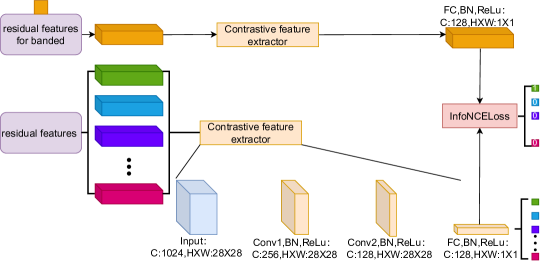
Figure 5: Contrastive Learning Architecture

Specifically, we abandon the original approach used in RelationNet, which concatenates feature vectors and lets the network learn to distinguish the similarity between two sets of features. Instead, we opt for using a multi-layer convolutional network to extract further representations of features. This allows us to obtain representations of the support set and the test set. We then employ InfoNCE[27] for contrastive learning. The formula for the InfoNCE loss is as Equation 3:

$$\text{InfoNCE Loss}=-\mathbb{E}_{x_{i}\in X_{s}}\left[\log\frac{\exp(f(x_{i})\cdot g(x_{j}))}{\sum_{x_{j}\in X_{t}}\exp(f(x_{i})\cdot g(x_{j}))}\right]$$ (3)

Here, $f(x_{i})$ and $g(x_{j})$ are the residual features of the support set and the test set, respectively. $x_{i}$ is a sample from the support set $X_{s}$, representing a category of anomaly, $x_{j}$ is a sample from the test set $X_{t}$.

By changing the network architecture and combining it with the InfoNCE loss, we can obtain a better classification network, resulting in better few-shot classification results.

4 Experiments

4.1 Experiments Details

4.1.1 Dataset

We have conducted experiments on the MVTec AD[28] dataset, which comprises fifteen different industrial products, covering various industrial production scenarios. Among them, the category "Toothbrush" is the only one that does not have specific defect categories. The other fourteen categories mostly have three to eight defect categories each, which are the subjects of our study.

Another dataset MVTev 3D AD[29] is also included in this paper, but we only use the 2D image to classify anomaly.

Other datasets for anomaly detection such as VisA[30], KolektorSDD[31], BTAD[32], etc. They don’t provide category of anomaly, as we don’t include them in this paper.

4.1.2 Evaluation Metrics

Since it is a classification problem, the metrics for classification tasks typically include accuracy, precision, recall, etc. Here, for simplicity, we only displayed accuracy. Subsequently, we will calculate the multi-class accuracy for each category of items. The overall classification accuracy is then calculated as the average accuracy of the 14 categories of items.

4.1.3 Implementation Details

For the n-shot problem, we select the first n sample from the dataset. Considering the stochastic nature of the downsampling algorithm in PatchCore, different random seeds result in different $\mathcal{M}$ bank, leading to significant fluctuations in classification results. Therefore, for all subsequent experiments involving $\mathcal{M}$, random seeds will be set to 1, 2, 3, 4, and 5, respectively, for five experiments. The average value will be calculated, and the sample standard deviation will be indicated, such as 48.11% $\pm 4.83\%$.

For the data generation, we only use 1 sample from every category in DTD dataset.

For the vanilla baseline and the Contrastive classifier, different pre-training and training strategies are adopted.

Pre-training involves training with the generated data defined by pseudo-categories. Both pre-training and fine-tuning use a learning rate of 0.0001 and the Adam optimizer.

For both the vanilla baseline and the contrastive classifier, the number of pseudo-categories used for pre-training is 10 (empirical value). Each pre-training iteration randomly selects a specified number of categories from the generated dataset, here is 10. After each iteration, the current training accuracy is recorded, and if the accuracy exceeds the threshold of 0.4 (empirical value), pre-training stops in order to avoid overfitting in generated dataset.

During fine-tuning, for the vanilla baseline, the real data is traversed for training 45 times. For the Contrastive classifier, during fine-tuning, the number of iterations varies depending on the task. For two-shot tasks, the real data is traversed 45 times; for three-shot tasks, it is traversed 25 times, and for four-shot and five-shot tasks, it is traversed 15 times. All of these are empirical value with several simple ablation experiments(not shown in this paper). N-shot means every category of defect has n samples

Both the vanilla baseline and the contrastive classifier require inputs with support sets and query sets simultaneously. For pre-training, with a sufficiently large dataset, samples can be randomly selected from a class of data, and the probability of overlap between support sets and query sets is negligible. For fine-tuning, as the dataset is relatively small, a group of samples needs to be extracted from the input data as the query set, and the remaining data is used as the support set. The training details for contrastive classifier is shown in Algorithm 1.

Data: Input residual features $\mathcal{M}$, shot number $S$, classes number $C$

Result: For each feature in $\mathcal{M}$, a query sample $\mathcal{Q}$ and its corresponding support set $\mathcal{S}$ are selected

// Sort features by category

$\mathcal{M}_{sorted}\leftarrow\{\}$;

for $i=1$ to $C$ do

       for $j=1$ to $S$ do

             Extract $j$th feature of category $i$ from $\mathcal{M}$ and append to $\mathcal{M}_{sorted}$;

            

       end for

      

end for

$\mathcal{M}\leftarrow\mathcal{M}_{sorted}$;

// Iterate over all features in $\mathcal{M}$

for each feature $\mathcal{F}$ in $\mathcal{M}$ do

       // Select current feature as the query sample and delete it from the bank

       $\mathcal{Q}\leftarrow\mathcal{F}$;

       $\mathcal{M}\leftarrow\mathcal{M}\setminus\mathcal{F}$;

       // Initialize support set for this query

       $\mathcal{S}\leftarrow\{\}$;

       $\mathcal{T}\leftarrow\{\}$;

       // Select one feature from each category to form the support set

       for $j=1$ to $S-1$ do

             for $i=1$ to $C$ do

                   $\mathcal{F}_{support}\leftarrow$ Select The jth Feature From ith Category($\mathcal{M}$, $i$, $j$);

                   $\mathcal{S}\leftarrow\mathcal{S}\cup\{\mathcal{F}_{support}\}$;

                  

             end for

            // Now, $\mathcal{Q}$ and $\mathcal{S}$ can be used for training or evaluation

            

       end for

      

end for

Algorithm 1 Feature Sorting and Query-Support Pair Generation

Additionally, the hyper parameters of the PatchCore section remain consistent with the original paper, i.e., the downsampling factor $p=10\%$.

4.2 Results

The comparison results are shown in Figure 6. The classification results of MvTec are shown in Table 1. Note that we assume all images to be tested are defective. Additionly, it is noted that when the number of shots reaches 4, there is a noticeable anomalous decrease in performance on MvTec AD dataset. Consequently, we also present the results of direct training without pretraining, i.e., without using generated data, in Table 3. It can be observed that when the number of shots exceeds 3, the significant gap between our synthesized data and real defects leads to a decrease in performance when using pretraining with synthesized data in four-shot scenarios. However, pretraining with synthesized data still yields better performance in the two-shot, three-shot and five-shot scenarios.

The results of MvTec 3D AD dataset are shown in Table 2.

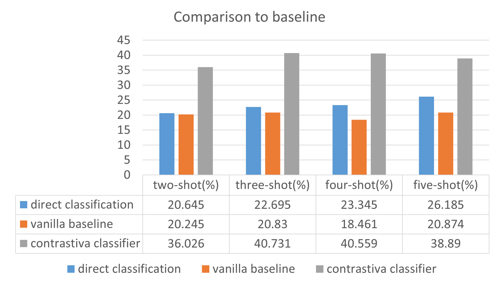
Figure 6: Comparison to baseline

Table 1: Contrastive-Classifier Results in MvTec AD Dataset. We especially use bold font if one reaches better performance compared with Table 3.

category	two-shot(%)	three-shot(%)	four-shot(%)	five-shot(%)	one-shot(%)
bottle	71.93 $\pm 2.48$	75.92 $\pm 1.32$	81.96 $\pm 4.25$	80.83 $\pm 6.82$	66.00 $\pm 5.08$
cable	29.21 $\pm 6.13$	35.00 $\pm 2.83$	38.67 $\pm 4.31$	42.69 $\pm 6.29$	13.09 $\pm 3.57$
capsule	39.79 $\pm 2.63$	38.72 $\pm 4.02$	42.02 $\pm 2.33$	47.38 $\pm 7.94$	22.12 $\pm 5.13$
carpet	27.34 $\pm 4.44$	29.19 $\pm 5.46$	23.77 $\pm 0.79$	21.25 $\pm 4.22$	23.81 $\pm 3.47$
grid	21.28 $\pm 0.00$	19.53 $\pm 1.06$	15.68 $\pm 2.26$	24.38 $\pm 6.40$	23.08 $\pm 4.51$
hazelnut	42.58 $\pm 3.34$	33.45 $\pm 3.13$	48.52 $\pm 6.86$	51.20 $\pm 3.03$	35.13 $\pm 9.67$
leather	29.76 $\pm 2.53$	34.03 $\pm 2.32$	34.44 $\pm 2.67$	38.51 $\pm 3.06$	21.84 $\pm 3.15$
metal nut	53.17 $\pm 1.93$	50.87 $\pm 1.35$	50.65 $\pm 2.06$	55.06 $\pm 4.27$	48.99 $\pm 3.43$
pill	34.80 $\pm 6.48$	31.00 $\pm 4.46$	27.61 $\pm 1.58$	28.49 $\pm 2.94$	22.13 $\pm 3.31$
screw	20.37 $\pm 2.38$	22.31 $\pm 1.26$	21.61 $\pm 1.53$	22.98 $\pm 3.25$	21.41 $\pm 3.65$
tile	52.43 $\pm 4.42$	57.10 $\pm 6.77$	59.06 $\pm 2.57$	63.05 $\pm 1.86$	28.61 $\pm 5.19$
transistor	43.13 $\pm 3.42$	70.00 $\pm 8.22$	55.83 $\pm 6.32$	66.00$\pm 10.84$	31.67 $\pm 7.24$
wood	24.00 $\pm 1.41$	29.33 $\pm 8.8$	40.00$\pm 10.90$	42.86 $\pm 5.34$	18.55 $\pm 5.52$
zipper	30.48 $\pm 4.09$	32.04 $\pm 5.23$	35.16 $\pm 5.10$	30.71 $\pm 6.96$	14.64 $\pm 1.85$
Average	37.16 $\pm 0.42$	39.89 $\pm 0.87$	41.07 $\pm 1.29$	43.96 $\pm 0.90$	27.93 $\pm 1.95$

Table 2: Contrastive-Classifier Results in MvTec 3D AD Dataset

category	two-shot(%)	three-shot(%)	four-shot(%)	five-shot(%)	one-shot(%)
bagel	29.50 $\pm 1.68$	27.37 $\pm 1.10$	29.45 $\pm 1.52$	31.47$\pm 2.23$	24.52 $\pm 3.82$
cable gland	35.95 $\pm 4.79$	30.13 $\pm 1.20$	34.36 $\pm 1.61$	36.95 $\pm 2.00$	24.58 $\pm 2.78$
carrot	27.54 $\pm 4.77$	31.97 $\pm 4.30$	34.29 $\pm 5.27$	35.14 $\pm 3.00$	29.45 $\pm 3.42$
cookie	34.53 $\pm 3.28$	35.39 $\pm 4.42$	38.29 $\pm 3.11$	34.70 $\pm 1.32$	23.63 $\pm 2.91$
dowel	34.17 $\pm 2.26$	26.95 $\pm 2.70$	39.09 $\pm 5.83$	40.00 $\pm 3.43$	28.60 $\pm 3.51$
foam	33.33 $\pm 3.93$	37.94 $\pm 5.24$	36.87 $\pm 3.77$	35.00 $\pm 2.36$	24.48 $\pm 5.23$
peach	36.37 $\pm 4.17$	30.00 $\pm 1.75$	31.11 $\pm 3.33$	35.78 $\pm 4.27$	29.02 $\pm 2.03$
potato	34.52 $\pm 3.95$	31.75 $\pm 2.88$	32.37 $\pm 2.56$	37.78 $\pm 1.81$	26.82 $\pm 2.74$
rope	40.00 $\pm 8.79$	59.33 $\pm 7.13$	72.63 $\pm 4.57$	74.82 $\pm 5.94$	36.97 $\pm 3.49$
tire	35.44$\pm 10.08$	36.80 $\pm 3.07$	41.41 $\pm 3.24$	-	29.64 $\pm 6.30$
Average	34.14 $\pm 0.77$	34.76 $\pm 1.08$	39.00 $\pm 1.49$	40.18 $\pm 1.08$	27.77 $\pm 1.19$

Table 3: Contrastive-Classifier Results in MVTev AD Dataset Without Pretraining

category	two-shot(%)	three-shot(%)	four-shot(%)	five-shot(%)
bottle	58.24 $\pm 3.59$	74.13 $\pm 7.28$	85.88 $\pm 3.23$	87.08 $\pm 2.28$
cable	35.79 $\pm 4.78$	33.82 $\pm 6.50$	42.67 $\pm 7.60$	41.15 $\pm 7.27$
capsule	38.18 $\pm 4.13$	36.60 $\pm 4.02$	42.47 $\pm 3.01$	46.67 $\pm 3.98$
carpet	21.26 $\pm 1.65$	21.89 $\pm 3.23$	23.48 $\pm 4.40$	23.44 $\pm 2.21$
grid	23.83 $\pm 4.61$	22.86 $\pm 2.71$	18.38 $\pm 4.44$	21.25 $\pm 1.40$
hazelnut	33.55 $\pm 2.65$	32.76 $\pm 4.04$	43.70 $\pm 2.81$	51.60 $\pm 5.90$
leather	29.27 $\pm 2.44$	30.91 $\pm 4.72$	31.94 $\pm 4.39$	32.84 $\pm 5.38$
metal nut	49.65 $\pm 2.68$	51.61 $\pm 2.03$	51.74 $\pm 3.29$	55.61 $\pm 3.44$
pill	29.76 $\pm 4.07$	31.33 $\pm 2.61$	31.33 $\pm 4.32$	28.49 $\pm 2.53$
screw	23.12 $\pm 1.99$	21.73 $\pm 3.94$	22.62 $\pm 1.15$	22.98 $\pm 3.25$
tile	41.89 $\pm 3.82$	51.01 $\pm 4.27$	58.75 $\pm 4.89$	64.07 $\pm 6.27$
transistor	49.38 $\pm 2.61$	70.71 $\pm 9.91$	62.50 $\pm 6.59$	56.00 $\pm 2.24$
wood	34.80 $\pm 6.72$	35.11$\pm 10.82$	45.50 $\pm 8.91$	42.86$\pm 11.95$
zipper	30.48 $\pm 4.36$	34.08 $\pm 6.83$	34.72 $\pm 4.23$	30.95 $\pm 4.98$
Average	35.56 $\pm 1.54$	39.18 $\pm 1.83$	42.55 $\pm 2.28$	43.21 $\pm 0.91$

Table 4: Overall Ablation Study

Direct	Baseline	Residual	Pretraining	Contrastive	Results(%)
✓					20.65
	✓	✓	✓		27.43
			✓	✓	34.60
		✓		✓	35.56
		✓	✓	✓	37.16

Table 5: The results of the effectiveness of residual representation

category	redisual(%)	without residual(%)
bottle	61.75$\pm 11.73$	50.88
cable	26.58$\pm 10.66$	25.00
capsule	35.75 $\pm 3.32$	24.24
carpet	20.76 $\pm 3.18$	20.25
grid	20.85 $\pm 3.49$	34.04
hazelnut	49.03$\pm 11.94$	50.00
leather	25.85 $\pm 4.76$	29.27
matal nut	49.41 $\pm 2.49$	50.59
pill	28.82 $\pm 7.06$	18.90
screw	22.57 $\pm 1.54$	22.02
tile	48.11 $\pm 4.83$	35.14
transistor	50.00$\pm 11.48$	56.25
wood	36.00 $\pm 7.35$	44.00
zipper	26.48 $\pm 3.83$	23.81
Average	36.03	34.60

Table 6: The effectiveness of contrastive learning

category	contrastive(%)	vanilla baseline(%)
bottle	58.95 $\pm 8.82$	61.41 $\pm 4.96$
cable	26.58$\pm 10.66$	15.53 $\pm 3.27$
capsule	35.75 $\pm 3.32$	22.02 $\pm 2.41$
carpet	20.76 $\pm 3.18$	24.05 $\pm 5.30$
grid	20.85 $\pm 3.49$	18.72 $\pm 3.16$
hazelnut	49.03$\pm 11.94$	33.23 $\pm 3.34$
leather	25.85 $\pm 4.76$	21.22 $\pm 6.77$
metal nut	49.41 $\pm 2.49$	47.76 $\pm 4.52$
pill	28.82 $\pm 7.06$	20.63 $\pm 4.18$
screw	22.57 $\pm 1.54$	19.27 $\pm 2.34$
tile	48.11 $\pm 4.83$	35.41 $\pm 6.37$
transistor	50.00$\pm 11.48$	32.51 $\pm 8.15$
wood	36.00 $\pm 7.35$	14.40 $\pm 4.98$
zipper	26.48 $\pm 3.83$	15.62 $\pm 1.86$
Average	36.03	27.43

Additionally, to demonstrate that the contrastive classifier we use indeed explicitly represents the features in an appropriate manner, we present the t-SNE plots of two categories in two-shot scenarios before and after contrastive classifier, as shown in Figure 7 and Figure 8.

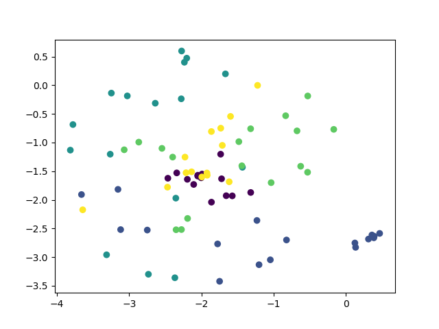
(a) t-sne for tile before contrastive classifier

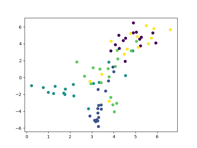
(b) t-sne for tile after contrastive classifier

Figure 7: t-sne for tile classification

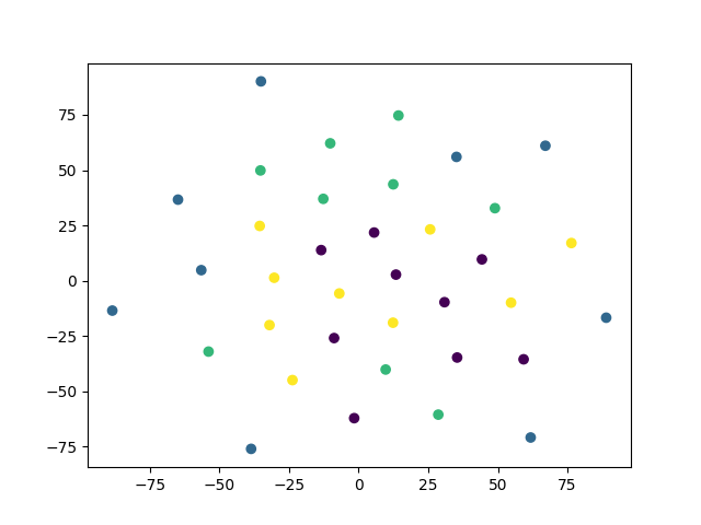
(a) t-sne for transistor before contrastive classifier

(b) t-sne for transistor after contrastive classifier

Figure 8: t-sne for transistor classification

4.3 Ablation Study

The overall ablation study is shown as Table 4, we only show the two-shot scenario’s result. The direct classification means we fine-tune the last fully connected layer of ResNet-50. As shown, the contrastive classifier with residual representation and pretraining achieves the best results in contrast to other methods.

4.3.1 Data Generation and Pretraining

As shown in Table 1 and Table 3. The results are as we have discussed in Subsection 4.2, in two-shot, three-shot and five-shot scenarios, pretraining with generated data shows better performance.

4.3.2 Residual Representations

In two-shot scenarios, we use contrasitive classifier with pretraning to compare the results between utilizing residual representations and not utilizing residual representations. The result is shown in Table 6. As we can see, we achieve better results when we use residual representations.

4.3.3 The Effectiveness of Contrasitive Classifier

In two-shot scenarios, we compare contrasitive classifier with pretraning to vanilla baseline with pretraining. And residual representations are adopted. The result is shown in Table 6. The contrastive classifier achieve better results in 11 items, and increase about 8% in average accuracy, which shows the effectiveness of contrastive learning for classifier.

5 Conclusion

In this paper, we explore the necessity of anomaly classification following anomaly detection, proposing a novel and valuable research task. We introduce a vanilla baseline for this task. Subsequently, in order to transfer few-shot learning to industrial applications, we propose a data generation method to enhance the model’s classification capability, achieving better results in two-shot and three-shot and five-shot scenarios. Furthermore, our proposed residual representation and contrastive learning based improvements to the vanilla baseline further enhance the model’s classification ability, improving classification accuracy.

Besides, our method can be easily embedded into any anomaly detection algorithm similar to PatchCore, e.g., Padim, SPADE, CPR.

6 Limitations

The data generation method proposed in this paper fails when there are four samples, indicating significant room for improvement in data generation methods for industrial data. We should anticipate more research in this area in the future.

Moreover, overall, the classification accuracy for defects in certain categories remains at the level of random guessing, indicating the difficulty of this task. Further research, such as metric-based or optimization-based methods, can be used to explore few-shot learning on industrial data.

Appendix

Appendix A Vanilla baseline Training Algorithm

Vanilla baseline can be difficult to train, we can train it similarly to Algorithm 1, but we found that it does not learn anything. Thus we apply a simpler training strategy described in Algorithm 2.

Appendix B The Complete Results of Vanilla Baseline

As shown in Table 7. We can find that the vanilla baseline is hard to train and doesn’t perform better as the number of samples increases. The results of vanilla baseline without pretraining are shown in Table 8. Pretraining makes it performs better in two-shot scenario.

Appendix C Another data generation method

The second method of image generation is largely similar to the first method, with the main difference being that the generated masks are specific-sized n-sided polygons, where $n\in{3,4,5,6}$. For texture images belonging to the same category from DTD, if they correspond to different-shaped masks, they will be labeled as different categories accordingly. Consequently, a maximum of $47*4$ defect images can be generated in this way. The initial purpose of this approach is to encourage the model to learn to distinguish between pseudo-defect texture information while also paying attention to the shape and edges of the defects. The results are shown in Table 9. But it doesn’t show better performance even worse than direct training due to overfitting in generated data.

Appendix D Other Results of Direct Classification

we will show the complete results here. As shown in Table 10

Appendix E The Complete Results of Contrastive Classifier without Residual Representation

Results are shown in Table 11

Appendix F MvTec 3D AD Results including good samples

In MvTec, PatchCore can achieve very high performance, while in MvTec 3D when we only use the RGB image it sometimes fails. Therefore in the whole workflow, there can be some good samples mixed with anomalous samples to be classified. We will show the results considerring normal samples in Table 12.

Appendix G Combine MAML with our model

We attempted some optimization-based few-shot learning methods, which are generally model-agnostic, such as MAML. The operational method is similar to MAML, but there is a slight difference due to our model inherently incorporating both the support set and the query set. This differs from MAML, which performs a first gradient descent on the support set before conducting a second gradient descent on the query set. Therefore, in our generated dataset, we selected a batch of categories as the support set for the first gradient descent and another batch of categories as the query set for the second gradient descent. This approach is consistent with the original concept of MAML and has been found to achieve better results in the two-shot scenario. The experimental data are shown in Table 13.

Appendix H Complete t-SNE results

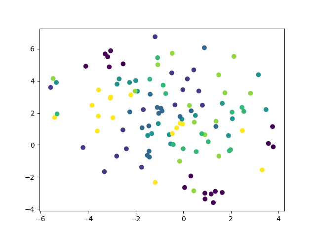
(a) t-sne for zipper before contrastive classifier

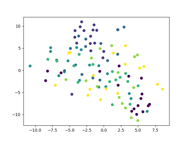
(b) t-sne for zipper after contrastive classifier

Figure 9: t-sne for zipper classification

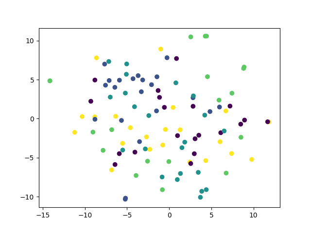
(a) t-sne for capsule before contrastive classifier

(b) t-sne for capsule after contrastive classifier

Figure 20: t-sne for capsule classification

We will show the tSNE results of the remaining 12 types of items. Only hazelnut, metal nut, bottle and capsule shows significant performance. As shown from Figure 9 to Figure 20

Data: Input residual features $\mathcal{M}$, shot number $S$, classes number $C$

// Sort features by category

$\mathcal{M}_{sorted}\leftarrow\{\}$;

for $i=1$ to $C$ do

       for $j=1$ to $S$ do

             Extract $j$th feature of category $i$ from $\mathcal{M}$ and append to $\mathcal{M}_{sorted}$;

            

       end for

      

end for

$\mathcal{M}\leftarrow\mathcal{M}_{sorted}$;

$\mathcal{S}\leftarrow\{\}$;

for $i=1$ to $C$ do

       Extract One feature $\mathcal{F}$ of category $i$ from $\mathcal{M}$;

       $\mathcal{S}\leftarrow\mathcal{S}\cup\{\mathcal{F}\}$;

       $\mathcal{M}\leftarrow\mathcal{M}\setminus\mathcal{F}$;

      

end for

// Iterate over all remainning features in $\mathcal{M}$

for each feature $\mathcal{F}$ in $\mathcal{M}$ do

       // Select current feature as the query sample and delete it from the bank

       $\mathcal{Q}\leftarrow\mathcal{F}$;

       $\mathcal{M}\leftarrow\mathcal{M}\setminus\mathcal{F}$;

       // Now, $\mathcal{Q}$ and $\mathcal{S}$ can be used for training or evaluation

      

end for

Algorithm 2 Training Method for Vanilla Baseline

Table 7: Complete Results of Vanilla Baseline

category	two-shot(%)	three-shot(%)	four-shot(%)	five-shot(%)	one-shot(%)
bottle	61.41 $\pm 4.96$	52.59 $\pm 12.18$	48.63 $\pm 11.30$	40.00 $\pm 4.75$	32.00 $\pm 0.74$
cable	15.53 $\pm 3.27$	18.53 $\pm 3.83$	19.00 $\pm 4.50$	18.46 $\pm 3.22$	13.57 $\pm 4.26$
capsule	22.02 $\pm 2.41$	20.43 $\pm 1.39$	20.22 $\pm 2.43$	21.18 $\pm 0.52$	17.50 $\pm 0.80$
carpet	24.05 $\pm 5.30$	20.00 $\pm 2.93$	17.97 $\pm 2.20$	18.13 $\pm 3.60$	21.43 $\pm 3.37$
grid	18.72 $\pm 3.16$	21.43 $\pm 3.76$	21.62 $\pm 7.88$	18.13 $\pm 4.64$	19.62 $\pm 5.16$
hazelnut	33.23 $\pm 3.34$	32.07 $\pm 3.97$	28.89 $\pm 4.46$	33.60 $\pm 3.85$	26.97 $\pm 1.97$
leather	21.22 $\pm 6.77$	19.48 $\pm 2.60$	23.33 $\pm 2.28$	20.60 $\pm 2.87$	23.45 $\pm 2.09$
metal nut	47.76 $\pm 4.52$	51.11 $\pm 2.56$	48.57 $\pm 5.92$	51.51 $\pm 3.43$	30.00 $\pm 4.27$
pill	20.63 $\pm 4.18$	20.83 $\pm 2.20$	19.65 $\pm 3.56$	18.87 $\pm 3.89$	6.12 $\pm 0.82$
screw	19.27 $\pm 2.34$	20.00 $\pm 2.19$	21.01 $\pm 0.45$	18.94 $\pm 2.31$	18.77 $\pm 1.00$
tile	35.41 $\pm 6.37$	26.09 $\pm 5.52$	25.31 $\pm 2.04$	27.12 $\pm 5.75$	24.56 $\pm 2.91$
transistor	32.51 $\pm 8.15$	36.43 $\pm 11.22$	36.67 $\pm 11.56$	32.00 $\pm 10.37$	27.78 $\pm 2.78$
wood	14.40 $\pm 4.98$	19.11 $\pm 9.89$	10.50 $\pm 3.26$	26.86 $\pm 15.20$	14.91 $\pm 1.99$
zipper	15.48 $\pm 2.11$	13.06 $\pm 3.18$	13.19 $\pm 2.05$	13.34 $\pm 1.00$	14.11 $\pm 0.98$
Average	27.43 $\pm 1.05$	26.51 $\pm 1.55$	25.42 $\pm 1.37$	25.62 $\pm 2.11$	20.77 $\pm 0.77$

Table 8: Complete Results of Vanilla Baseline without Pretraining

category	two-shot(%)	three-shot(%)	four-shot(%)	five-shot(%)
bottle	39.04 $\pm 7.64$	39.26 $\pm 6.06$	37.25 $\pm 4.60$	41.67 $\pm 8.72$
cable	19.03 $\pm 2.86$	18.24 $\pm 7.96$	14.33 $\pm 4.95$	15.38 $\pm 4.90$
capsule	23.63 $\pm 2.21$	20.43 $\pm 1.90$	22.92 $\pm 5.60$	21.19 $\pm 5.28$
carpet	21.52 $\pm 4.10$	19.19 $\pm 4.82$	18.84 $\pm 2.90$	20.94 $\pm 3.24$
grid	22.13 $\pm 4.90$	22.86 $\pm 5.73$	19.46 $\pm 6.45$	16.88 $\pm 2.79$
hazelnut	32.76 $\pm 6.71$	30.26 $\pm 3.29$	31.85 $\pm 4.79$	29.47 $\pm 2.72$
leather	20.16 $\pm 2.70$	19.22 $\pm 3.24$	21.11 $\pm 3.01$	18.81 $\pm 4.08$
metal nut	42.82 $\pm 9.79$	49.88 $\pm 2.24$	50.39 $\pm 1.93$	49.32 $\pm 4.33$
pill	15.12 $\pm 5.58$	13.50 $\pm 6.70$	12.74 $\pm 5.79$	18.11 $\pm 4.08$
screw	18.35 $\pm 1.59$	23.73 $\pm 3.80$	19.80 $\pm 3.82$	20.42 $\pm 3.64$
tile	33.24 $\pm 3.65$	30.44 $\pm 4.10$	27.23 $\pm 6.48$	27.46 $\pm 4.55$
transistor	25.00 $\pm 9.63$	43.57 $\pm 11.68$	39.17 $\pm 9.13$	30.00 $\pm 5.00$
wood	22.80 $\pm 7.01$	29.78 $\pm 9.37$	29.00 $\pm 6.27$	26.86 $\pm 6.88$
zipper	17.33 $\pm 2.64$	12.65 $\pm 1.55$	15.42 $\pm 4.37$	13.10 $\pm 2.23$
Average	25.61 $\pm 0.74$	28.12 $\pm 1.40$	25.71 $\pm 0.81$	25.63 $\pm 1.17$

Table 9: Contrastive-Classifier Results in MvTec AD Dataset by new data generation method

category	two-shot(%)	three-shot(%)	four-shot(%)	five-shot(%)
bottle	67.37 $\pm 2.66$	74.07 $\pm 3.93$	71.77 $\pm 6.29$	76.67 $\pm 6.81$
cable	30.00 $\pm 5.22$	32.63 $\pm 6.17$	34.33 $\pm 6.08$	39.91 $\pm 5.06$
capsule	40.00 $\pm 1.97$	39.79 $\pm 3.73$	41.12 $\pm 2.82$	45.24 $\pm 4.69$
carpet	23.54 $\pm 2.12$	22.97 $\pm 6.19$	24.93 $\pm 6.27$	19.06 $\pm 2.57$
grid	27.66 $\pm 1.51$	22.86 $\pm 3.61$	22.16 $\pm 4.84$	21.88 $\pm 6.63$
hazelnut	50.00 $\pm 10.26$	41.38 $\pm 2.44$	49.26 $\pm 7.92$	57.20 $\pm 5.40$
leather	26.34 $\pm 2.81$	31.43 $\pm 4.34$	29.72 $\pm 3.20$	31.34 $\pm 6.76$
metal nut	47.77 $\pm 1.34$	49.38 $\pm 3.38$	52.21 $\pm 1.42$	53.70 $\pm 3.12$
pill	30.55 $\pm 4.74$	29.50 $\pm 3.04$	29.03 $\pm 1.70$	28.68 $\pm 0.52$
screw	24.22 $\pm 2.95$	21.35 $\pm 1.26$	20.20 $\pm 2.02$	20.00 $\pm 3.87$
tile	42.70 $\pm 8.58$	57.10 $\pm 6.20$	45.00 $\pm 12.37$	42.03 $\pm 15.41$
transistor	35.00 $\pm 6.40$	63.57 $\pm 8.15$	55.83 $\pm 10.87$	53.00 $\pm 12.55$
wood	31.60 $\pm 5.90$	36.45 $\pm 10.49$	39.50 $\pm 8.73$	34.86 $\pm 15.96$
zipper	28.00 $\pm 7.05$	20.82 $\pm 2.66$	23.52 $\pm 6.44$	20.24 $\pm 3.67$
Average	36.05 $\pm 1.30$	38.81 $\pm 0.71$	38.47 $\pm 1.96$	38.80 $\pm 2.10$

Table 10: Complete Results of Direct Classification

category	two-shot(%)	three-shot(%)	four-shot(%)	five-shot(%)	one-shot(%)
bottle	26.32	29.63	39.22	33.33	33.33
cable	10.53	14.71	8.33	19.23	15.48
capsule	22.22	23.40	33.71	29.76	23.08
carpet	20.25	18.92	21.74	23.44	20.24
grid	21.28	21.43	21.62	21.88	19.23
hazelnut	33.87	31.03	38.89	38.00	25.76
leather	14.63	22.08	16.67	22.39	21.84
metal nut	28.24	37.04	28.57	32.88	17.98
pill	21.26	15.83	19.47	16.04	14.18
screw	16.51	18.27	16.16	20.21	16.67
tile	17.57	23.19	31.25	37.29	21.51
transistor	6.25	21.43	20.83	25.00	25.00
wood	32.00	24.44	15.00	25.71	18.18
zipper	18.10	16.33	15.38	21.43	16.07
Average	20.65	22.70	23.35	26.19	20.61

Table 11: The Complete Results of Contrastive Classifier without Residual Representation

category	two-shot(%)	three-shot(%)	four-shot(%)	five-shot(%)	one-shot(%)
bottle	50.88	70.37	68.63	66.67	43.33
cable	25.00	17.65	11.67	13.46	11.90
capsule	24.24	30.85	26.97	33.33	20.18
carpet	20.25	22.97	23.19	23.44	21.43
grid	34.04	23.81	21.62	18.75	19.23
hazelnut	50.00	36.21	37.04	30.00	31.82
leather	29.27	31.17	19.44	32.84	14.94
metal nut	50.59	48.15	50.65	27.40	47.19
pill	18.90	18.33	20.35	19.81	20.15
screw	22.02	22.12	21.21	21.28	20.18
tile	35.14	33.33	35.94	30.51	27.85
transistor	56.25	64.29	45.83	35.00	38.89
wood	44.00	46.67	40.00	22.86	27.27
zipper	23.81	26.53	15.38	17.86	17.86
Average	34.60	35.18	31.28	28.09	25.87

Table 12: Results in MvTec 3D AD Dataset including normal samples

category	two-shot(%)	three-shot(%)	four-shot(%)	five-shot(%)	one-shot(%)
bagel	24.60 $\pm 4.22$	26.10 $\pm 3.60$	22.67 $\pm 2.17$	28.47$\pm 1.53$	24.95 $\pm 2.17$
cable gland	33.47 $\pm 3.98$	23.66 $\pm 1.32$	31.81 $\pm 1.61$	34.46 $\pm 1.37$	20.00 $\pm 2.13$
carrot	24.22 $\pm 4.47$	29.08 $\pm 7.39$	29.19 $\pm 3.53$	29.46 $\pm 3.80$	24.71 $\pm 2.33$
cookie	29.75 $\pm 2.48$	29.65 $\pm 4.38$	33.15 $\pm 3.40$	33.02 $\pm 3.13$	20.32 $\pm 2.67$
dowel	26.83 $\pm 4.22$	25.22 $\pm 2.04$	33.64 $\pm 4.90$	35.81 $\pm 4.93$	24.48 $\pm 3.78$
foam	34.89 $\pm 2.31$	38.12 $\pm 2.95$	34.50 $\pm 3.60$	30.67 $\pm 6.11$	21.68 $\pm 1.41$
peach	29.18 $\pm 1.89$	27.86 $\pm 3.34$	27.32 $\pm 2.72$	27.85 $\pm 2.02$	22.83 $\pm 1.47$
potato	27.50 $\pm 3.23$	35.35 $\pm 2.47$	34.68 $\pm 4.09$	36.18 $\pm 2.30$	22.20 $\pm 4.56$
rope	49.25 $\pm 11.08$	48.76 $\pm 7.27$	61.88 $\pm 10.04$	67.41 $\pm 4.06$	31.34 $\pm 1.17$
tire	34.90 $\pm 3.58$	35.26 $\pm 4.27$	35.00 $\pm 4.44$	-	23.74 $\pm 4.41$
Average	31.46 $\pm 1.56$	31.91 $\pm 1.91$	34.38 $\pm 1.94$	35.92 $\pm 1.21$	23.63 $\pm 1.05$

Table 13: Contrastive-Classifier Results in MvTec AD Dataset With MAML Training Tricks.

category	two-shot(%)	three-shot(%)	four-shot(%)	five-shot(%)	one-shot(%)
bottle	68.07 $\pm 3.80$	75.93 $\pm 1.31$	83.14 $\pm 4.72$	77.50 $\pm 4.52$	55.67 $\pm 3.03$
cable	32.90 $\pm 3.84$	32.94 $\pm 4.37$	40.00 $\pm 4.08$	38.85 $\pm 9.06$	18.57 $\pm 4.34$
capsule	38.78 $\pm 2.33$	36.38 $\pm 2.05$	38.88 $\pm 2.58$	44.05 $\pm 4.29$	25.38 $\pm 0.86$
carpet	25.57 $\pm 1.06$	26.49 $\pm 2.63$	25.51 $\pm 4.17$	24.06 $\pm 2.37$	21.43 $\pm 3.15$
grid	21.28 $\pm 0.00$	23.33 $\pm 3.91$	21.08 $\pm 2.96$	20.00 $\pm 1.71$	16.92 $\pm 3.44$
hazelnut	37.74 $\pm 7.70$	28.97 $\pm 2.56$	40.00 $\pm 6.75$	48.80 $\pm 11.01$	28.48 $\pm 3.92$
leather	23.66 $\pm 1.85$	32.99 $\pm 1.97$	35.28 $\pm 2.33$	29.71 $\pm 6.76$	19.54 $\pm 2.30$
metal nut	48.00 $\pm 2.26$	49.38 $\pm 1.51$	52.99 $\pm 3.10$	56.98 $\pm 2.67$	51.46 $\pm 2.16$
pill	32.60 $\pm 4.12$	30.50 $\pm 2.74$	28.67 $\pm 1.34$	27.55 $\pm 1.03$	23.73 $\pm 3.09$
screw	24.77 $\pm 3.84$	23.46 $\pm 3.01$	19.39 $\pm 4.60$	20.07 $\pm 4.26$	20.70 $\pm 4.33$
tile	47.30 $\pm 4.48$	53.62 $\pm 4.91$	54.38 $\pm 4.04$	56.95 $\pm 4.25$	25.32 $\pm 5.14$
transistor	56.25 $\pm 3.83$	66.43 $\pm 4.07$	60.83 $\pm 6.97$	66.00 $\pm 7.42$	35.00 $\pm 6.69$
wood	42.40 $\pm 10.99$	33.78 $\pm 8.23$	49.50 $\pm 7.16$	37.71 $\pm 9.35$	23.64 $\pm 7.82$
zipper	27.24 $\pm 2.48$	28.98 $\pm 2.94$	40.22 $\pm 4.51$	23.10 $\pm 4.80$	14.46 $\pm 2.63$
Average	37.61 $\pm 0.93$	38.80 $\pm 0.76$	42.13 $\pm 0.81$	41.16 $\pm 2.19$	27.17 $\pm 1.15$

(a) t-sne for wood before contrastive classifier

(b) t-sne for wood after contrastive classifier

Figure 10: t-sne for wood classification

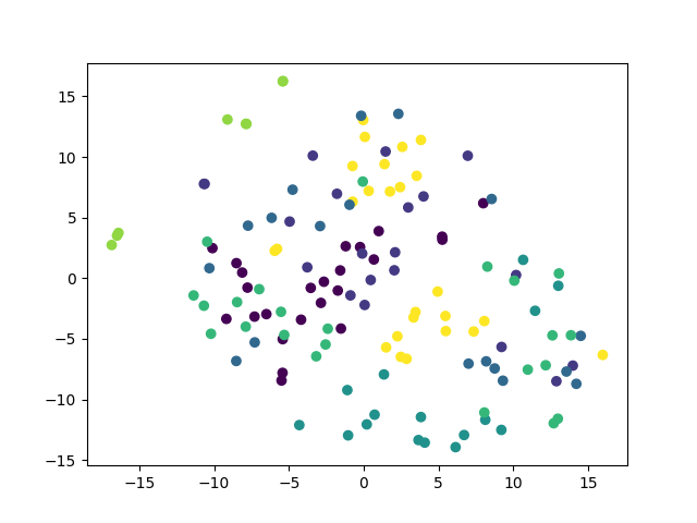
(a) t-sne for pill before contrastive classifier

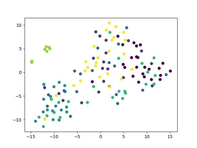
(b) t-sne for pill after contrastive classifier

Figure 11: t-sne for pill classification

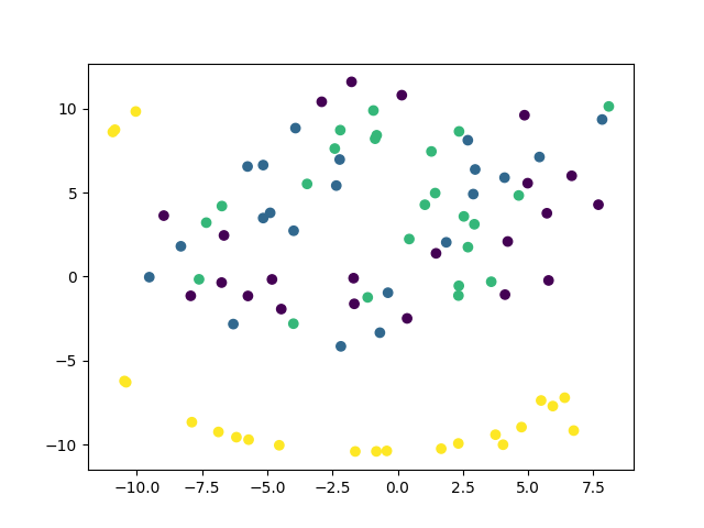
(a) t-sne for metal nut before contrastive classifier

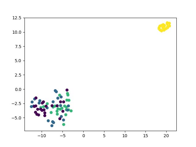
(b) t-sne for metal nut after contrastive classifier

Figure 12: t-sne for metal nut classification

(a) t-sne for leather before contrastive classifier

(b) t-sne for leather after contrastive classifier

Figure 13: t-sne for leather classification

(a) t-sne for hazelnut before contrastive classifier

(b) t-sne for hazelnut after contrastive classifier

Figure 14: t-sne for hazelnut classification

(a) t-sne for grid before contrastive classifier

(b) t-sne for grid after contrastive classifier

Figure 15: t-sne for grid classification

(a) t-sne for carpet before contrastive classifier

(b) t-sne for carpet after contrastive classifier

Figure 16: t-sne for carpet classification

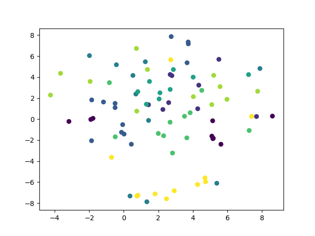
(a) t-sne for cable before contrastive classifier

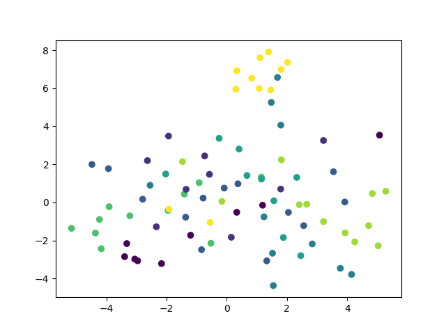
(b) t-sne for cable after contrastive classifier

Figure 17: t-sne for cable classification

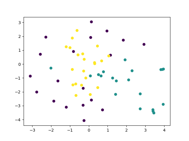
(a) t-sne for bottle before contrastive classifier

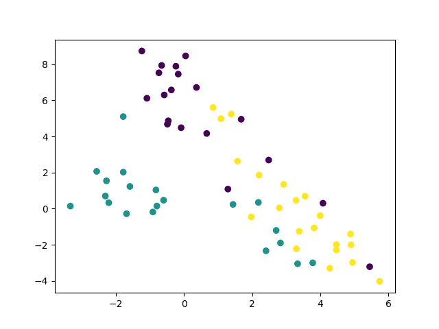
(b) t-sne for bottle after contrastive classifier

Figure 18: t-sne for bottle classification

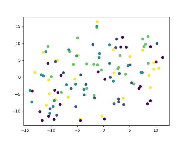
(a) t-sne for screw before contrastive classifier

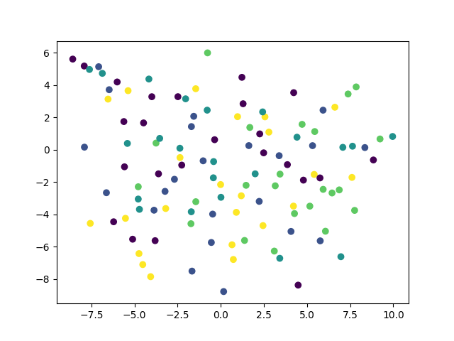
(b) t-sne for screw after contrastive classifier

Figure 19: t-sne for screw classification

References

- [1] Karsten Roth, Latha Pemula, Joaquin Zepeda, Bernhard Schölkopf, Thomas Brox, and Peter Gehler. Towards total recall in industrial anomaly detection. In CVPR, pages 14318–14328, 2022.
- [2] Jongheon Jeong, Yang Zou, Taewan Kim, Dongqing Zhang, Avinash Ravichandran, and Onkar Dabeer. Winclip: Zero-/few-shot anomaly classification and segmentation. In CVPR, pages 19606–19616, 2023.
- [3] Yisheng Song, Ting Wang, Puyu Cai, Subrota K Mondal, and Jyoti Prakash Sahoo. A comprehensive survey of few-shot learning: Evolution, applications, challenges, and opportunities. ACM Computing Surveys, 2023.
- [4] Chelsea Finn, Pieter Abbeel, and Sergey Levine. Model-agnostic meta-learning for fast adaptation of deep networks. In ICML, pages 1126–1135. PMLR, 2017.
- [5] Ling Yang, Liangliang Li, Zilun Zhang, Xinyu Zhou, Erjin Zhou, and Yu Liu. Dpgn: Distribution propagation graph network for few-shot learning. In CVPR, pages 13390–13399, 2020.
- [6] Gregory Koch, Richard Zemel, Ruslan Salakhutdinov, et al. Siamese neural networks for one-shot image recognition. In ICML deep learning workshop, volume 2. Lille, 2015.
- [7] Oriol Vinyals, Charles Blundell, Timothy Lillicrap, Daan Wierstra, et al. Matching networks for one shot learning. NeurIPS, 29, 2016.
- [8] Jake Snell, Kevin Swersky, and Richard Zemel. Prototypical networks for few-shot learning. NeurIPS, 30, 2017.
- [9] Flood Sung, Yongxin Yang, Li Zhang, Tao Xiang, Philip HS Torr, and Timothy M Hospedales. Learning to compare: Relation network for few-shot learning. In CVPR, pages 1199–1208, 2018.
- [10] Niv Cohen and Yedid Hoshen. Sub-image anomaly detection with deep pyramid correspondences, 2021.
- [11] Alex Krizhevsky, Ilya Sutskever, and Geoffrey E Hinton. Imagenet classification with deep convolutional neural networks. NeurIPS, 25, 2012.
- [12] Thomas Defard, Aleksandr Setkov, Angelique Loesch, and Romaric Audigier. Padim: a patch distribution modeling framework for anomaly detection and localization. In ICPR, pages 475–489. Springer, 2021.
- [13] Hanxi Li, Jianfei Hu, Bo Li, Hao Chen, Yongbin Zheng, and Chunhua Shen. Target before shooting: Accurate anomaly detection and localization under one millisecond via cascade patch retrieval. arXiv preprint arXiv:2308.06748, 2023.
- [14] Jeeho Hyun, Sangyun Kim, Giyoung Jeon, Seung Hwan Kim, Kyunghoon Bae, and Byung Jun Kang. Reconpatch: Contrastive patch representation learning for industrial anomaly detection. In CVPR, pages 2052–2061, 2024.
- [15] Hui Zhang, Zuxuan Wu, Zheng Wang, Zhineng Chen, and Yu-Gang Jiang. Prototypical residual networks for anomaly detection and localization. In CVPR, pages 16281–16291, June 2023.
- [16] Kihyuk Sohn, Jinsung Yoon, Chun-Liang Li, Chen-Yu Lee, and Tomas Pfister. Anomaly clustering: Grouping images into coherent clusters of anomaly types. In WACV, pages 5479–5490, 2023.
- [17] Yanfeng Gong, Jun Luo, Hongliang Shao, and Zhixue Li. A transfer learning object detection model for defects detection in x-ray images of spacecraft composite structures. Composite Structures, 284:115136, 2022.
- [18] Junnan Li, Yongkang Wong, Qi Zhao, and Mohan S Kankanhalli. Learning to learn from noisy labeled data. In CVPR, pages 5051–5059, 2019.
- [19] Yiwei Lu, Frank Yu, Mahesh Kumar Krishna Reddy, and Yang Wang. Few-shot scene-adaptive anomaly detection. In ECCV, pages 125–141. Springer, 2020.
- [20] Ruibing Hou, Hong Chang, Bingpeng Ma, Shiguang Shan, and Xilin Chen. Cross attention network for few-shot classification. NeurIPS, 32, 2019.
- [21] Kaiming He, Xiangyu Zhang, Shaoqing Ren, and Jian Sun. Deep residual learning for image recognition. In CVPR, pages 770–778, 2016.
- [22] Vitjan Zavrtanik, Matej Kristan, and Danijel Skočaj. Draem-a discriminatively trained reconstruction embedding for surface anomaly detection. In ICCV, pages 8330–8339, 2021.
- [23] Mircea Cimpoi, Subhransu Maji, Iasonas Kokkinos, Sammy Mohamed, and Andrea Vedaldi. Describing textures in the wild. In CVPR, pages 3606–3613, 2014.
- [24] Carsten Rother, Vladimir Kolmogorov, and Andrew Blake. " grabcut" interactive foreground extraction using iterated graph cuts. TOG, 23(3):309–314, 2004.
- [25] Ting Chen, Simon Kornblith, Mohammad Norouzi, and Geoffrey Hinton. A simple framework for contrastive learning of visual representations. In ICML, pages 1597–1607. PMLR, 2020.
- [26] Kaiming He, Haoqi Fan, Yuxin Wu, Saining Xie, and Ross Girshick. Momentum contrast for unsupervised visual representation learning. In CVPR, pages 9729–9738, 2020.
- [27] Aaron van den Oord, Yazhe Li, and Oriol Vinyals. Representation learning with contrastive predictive coding. arXiv preprint arXiv:1807.03748, 2018.
- [28] Paul Bergmann, Michael Fauser, David Sattlegger, and Carsten Steger. Mvtec ad – a comprehensive real-world dataset for unsupervised anomaly detection. In CVPR, June 2019.
- [29] Paul Bergmann, Xin Jin, David Sattlegger, and Carsten Steger. The mvtec 3d-ad dataset for unsupervised 3d anomaly detection and localization. arXiv preprint arXiv:2112.09045, 2021.
- [30] Yang Zou, Jongheon Jeong, Latha Pemula, Dongqing Zhang, and Onkar Dabeer. Spot-the-difference self-supervised pre-training for anomaly detection and segmentation. In European Conference on Computer Vision, pages 392–408. Springer, 2022.
- [31] Domen Tabernik, Samo Šela, Jure Skvarč, and Danijel Skočaj. Segmentation-based deep-learning approach for surface-defect detection. Journal of Intelligent Manufacturing, 31(3):759–776, 2020.
- [32] Pankaj Mishra, Riccardo Verk, Daniele Fornasier, Claudio Piciarelli, and Gian Luca Foresti. Vt-adl: A vision transformer network for image anomaly detection and localization. In 2021 IEEE 30th International Symposium on Industrial Electronics (ISIE), pages 01–06. IEEE, 2021.