Mean-field Chaos Diffusion Models

Abstract

In this paper, we introduce a new class of score-based generative models (SGMs) designed to handle high-cardinality data distributions by leveraging concepts from mean-field theory. We present mean-field chaos diffusion models (MF-CDMs), which address the curse of dimensionality inherent in high-cardinality data by utilizing the propagation of chaos property of interacting particles. By treating high-cardinality data as a large stochastic system of interacting particles, we develop a novel score-matching method for infinite-dimensional chaotic particle systems and propose an approximation scheme that employs a subdivision strategy for efficient training. Our theoretical and empirical results demonstrate the scalability and effectiveness of MF-CDMs for managing large high-cardinality data structures, such as 3D point clouds.

APAppendix References *

1 Introduction

Generative models serve as a fundamental focus in machine learning, aiming to learn a high-dimensional probability density function. Among the contenders such as Normalizing flows (Rezende & Mohamed, 2015) and energy-based models (Zhao et al., 2016), Score-based Generative Models (SGMs), especially have gained widespread recognition of their capabilities on various domains, such as images (Song et al., 2021b), time-series (Tashiro et al., 2021; Park et al., 2023), graphs (Jo et al., 2022) and point-clouds (Zeng et al., 2022). The key idea of SGMs is to conceptualize a combination of forward and reverse diffusion processes as generative models. In forward dynamics, the data density is progressively corrupted by following a Markov probability trajectory, eventually transformed into Gaussian density. Consequently, denoising score networks sequentially remove noises in the reverse dynamics, aiming to restore the original state.

Despite the remarkable empirical successes, recent theoretical studies (De Bortoli, 2022; Chen et al., 2023) have highlighted the limitations on the scalability of SGMs when applied to high-dimensional and high-cardinality data structures. To tackle the challenge, a series of research (Lim et al., 2023; Kerrigan et al., 2023; Dutordoir et al., 2023; Hagemann et al., 2023) broadens the scope of diffusion models, introducing new methods for data representation in an infinite-dimensional function space. These macroscopic approaches fully mitigate dimensionality issues in diffusion modeling; however, they make strong assumptions on the function-valued representations of the input data, which limits their applicability to practical settings such as modeling 3D point clouds.

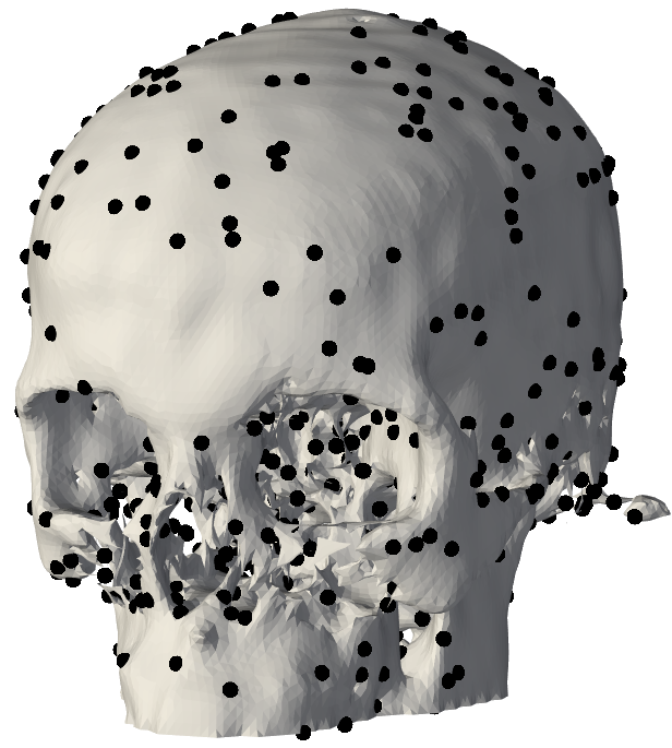
Figure 1: 3D representations of $(\nu^{N},\mu)$.

This paper introduces another strategy to manage high cardinality data through the lens of mean-field theory (MFT) and restructure existing SGMs. MFT has long been recognized as a powerful analytical tool for large-scale particle systems in multiple disciplines, such as statistical physics (Kadanoff, 2009), biology (Koehl & Delarue, 1994), and macroeconomics (Lachapelle et al., 2010). Among the diverse concepts developed in MFT, our interest specifically focuses on the property called propagation of chaos (PoC) (Sznitman, 1991a; Gottlieb, 1998), which describes statistical independency and symmetry in proximity to the mean-field limit of large-particle system. While the direct integration of PoC into conventional SGMs poses a considerable challenge due to the infinite dimensionality, our systematic approach begins by defining denoising models with interacting $N$-particle diffusion dynamics (i.e., , $\nu^{N}$, block dots, Fig. 1). We then explore ways to approximate its mean-field limit ($\textit{i}.\textit{e}.,N\rightarrow\infty,\mu$, organ surface), which can possess extensive representational capabilities. This work is centered on two key contributions to achieve this:

• Mean-field Score Matching. We introduce a variational framework on Wasserstein space by applying the Itô-Wentzell-Lions formula and derive a mean-field score matching (MF-SM) to generalize conventional SGMs for mean-field particle system. We provide mean-field analysis on the asymptotic behavior of the proposed novel framework to elucidate the effectiveness in learning large cardinality data distribution.

• Subdivision for Efficiency. For the ease of computational complexity, we introduce a subdivision of chaotic entropy, which establishes piece-wise discontinuous gradient flows and efficiently approximates the true discrepancy in a divide-and-conquer manner.

2 Mean-field Chaos Diffusion Models

2.1 Score-based Generative Models

Before presenting our proposed method, we provide a brief background on SGMs. For notations not discussed, refer to the detailed descriptions in Appendix.

Let us consider a probabilistic space $(\mathcal{Y},\mathcal{F}_{t},\mathbb{P})$ and two respective diffusion paths for variables $t$ and $u\coloneqq T-t$.

$$d\mathbf{X}_{u}=f_{u}(\mathbf{X}_{u})du+\sigma_{u}dB_{u},\quad\mathbf{X}_{u},\mathbf{X}_{t}\in\mathcal{Y},$$ (1)

$$d\mathbf{X}_{t}=\left[f_{t}(\mathbf{X}_{t})-\sigma_{t}^{2}\nabla\log\zeta_{t}(\mathbf{X}_{t})\right]dt+\sigma_{t}dB_{t}.$$ (2)

A pair of Markovian probability measures $(\zeta_{s},\nu_{t})$ corresponding to the system of the above SDEs, called forward-reverse SDEs (i.e., FR-SDEs), illustrates noising and denoising processes, respectively. A primitive form of the standard objective of SGMs is to minimize the discrepancy (e.g., relative entropy, $\tilde{\mathcal{H}}$) between data generative model $\nu_{T}$ and target data $\zeta_{0}$ at the terminal state of reverse dynamics, $t=T$:

$$\mathbf{(P0)}\quad\min_{\nu_{[0,T]}}\tilde{\mathcal{H}}[\nu_{T}|\zeta_{0}],$$ (3)

where $\nu_{[0,T]}$ denotes a path measure on the interval $[0,T]$. As the direct calculation is intractable, Song et al. (2021b) have shown that the optimization of an alternative tractable formulation, known as score matching objective, can minimize the discrepancy between $\nu_{T}$ and $\zeta_{0}$. The goal of SGMs is then to train a score network $\mathbf{s}_{\theta}$ to approximate a score function $(\textit{i}.\textit{e}.,\nabla\log\zeta_{t})$:

$$\mathcal{J}_{SM}(\theta)\propto\mathbb{E}_{t,\mathbf{X}_{t}}\left[\norm{\mathbf{s}_{\theta}(t,\mathbf{X}_{t})-\nabla\log\zeta_{t}(\mathbf{X}_{t})}^{2}\right].$$ (4)

Given the basic machinery defined above, one question naturally arises considering the goal outlined in the introduction:

Q1. How can we restructure existing diffusion models to preserve robust performance when $\mathbf{dim}(\mathcal{Y})\rightarrow\infty$?

Throughout the paper, we address this fundamental question using principles of MFT. As a first step, we begin with dissecting a decomposition of generic FR-SDEs defined on $\mathcal{Y}\leavevmode\nobreak\ (\textit{e}.\textit{g}.,\mathbb{R}^{Nd})$ into the mean-field interacting $N$-particle system on the space $\mathcal{X}\leavevmode\nobreak\ (\textit{e}.\textit{g}.,\mathbb{R}^{d})$.

2.2 Mean-field Stochastic Differential Equations

Our new definition of SDEs called mean-field stochastic differential equations (MF-SDEs) takes microscopic perspective to model diffusion processes:

Definition 2.1.

(Mean-field SDEs). For the atomless Polish space $\mathcal{X}$, let $\{B_{t}^{i,N}\}_{i\leq N}$ be a set of independent Wiener processes on probability space $(\mathcal{X},\mathcal{F}_{t},\mathbb{P})$. Then, we define the $N$-particle system as follows:

$$d\mathbf{X}_{u}^{i,N}=f_{s}(\mathbf{X}_{u}^{i,N})du+\sigma_{u}dB_{u}^{i,N},\quad\mathbf{X}_{u},\mathbf{X}_{t}\in\mathcal{X},$$ (5)

$$d\mathbf{X}_{t}^{i,N}=[f_{t}(\mathbf{X}_{t}^{i,N})-\sigma_{t}^{2}\nabla\log\zeta_{t}(\mathbf{X}_{t}^{i,N})]dt+\sigma_{t}dB_{t}^{i,N},$$ (6)

where the initial states of each dynamics is i.i.d. standard Gaussian random vectors, $\textit{i}.\textit{e}.,\mathbf{X}_{0}^{i,N}\sim\mathcal{N}[\mathbf{I}_{d}]$.

The proposed dynamics explicitly delineate the $N$ individual rules of each particle, modeling detailed inter-associations between particles. Upon the structure of MF-SDEs in Definition 2.1, the $N$-particle system is endowed with weak probabilistic structure $\varrho_{t}^{N}$ in the $Nd$-dimensional coordinate system $\mathbf{x}^{N}=(\mathbf{x}_{1},\cdots,\mathbf{x}_{N})\in\mathcal{X}^{N}$ and admits a joint density defined as following:

$$\mathbf{X}_{t}^{N}\sim\nu_{t}^{N}\coloneqq\mathbf{Law}(\mathbf{X}_{t}^{1,N},\cdots\mathbf{X}_{t}^{N,N})=\varrho^{N}_{t}d\mathbf{x}^{N},$$ (7)

$$\varrho^{M,N}_{t}(\mathbf{x}^{M})=\int_{\mathcal{X}^{N-M}}\varrho^{N}_{t}(\mathbf{x}^{N})d\mathbf{x}_{M+1}\cdots d\mathbf{x}_{N}.$$ (8)

Furthermore, a set of $N$ particles in the proposed system is exchangeable, satisfying the following symmetry property for any given permutation $\tau\in S_{N}$:

$$\varrho^{N}_{t}(\mathbf{x}_{1},\cdots,\mathbf{x}_{N})=\varrho^{N}_{t}(\mathbf{x}_{\tau(1)},\cdots,\mathbf{x}_{\tau(N)}).$$ (9)

Empirical Measures as Data. Compared to the data description $\nu_{t}$ of the macroscopic approach in FR-SDE, our framework interprets a single instance (e.g., point cloud) as an empirical random measure $\nu_{t}^{N}$, in which particles (e.g., point) are represented as marginal random variables $\mathbf{X}_{t}^{i,N}$,

$$\underbrace{\mathcal{P}_{2}(\mathcal{Y})\ni\nu_{T}}_{\text{FR-SDEs}}\leavevmode\nobreak\ \leftrightarrow\leavevmode\nobreak\ \underbrace{\nu_{T}^{N}\coloneqq\varrho^{N}d\mathbf{x}^{N}\in\mathcal{P}(\mathcal{P}_{2}(\mathcal{X}^{N}))}_{\text{MF-SDEs}}.$$ (10)

It is clear from the context that the term ‘cardinality’ stands for the degree of $N$, and the proposed interpretation features two key points. First, our method simply augments the particle count $N\uparrow$ in handling high-resolution data instances, keeping the dimensionality $d=\mathbf{dim}(\mathcal{X})$. This modeling can explicitly expose the effect of increasing cardinality in the analysis as opposite to FR-SDEs, which adjust the dimensionality of the ambient space $Nd=\mathbf{dim}(\mathcal{Y})$ without comprehensive details. Second, data representations $\nu_{T}^{N}$ naturally inherit the permutation invariance which is essential for efficient learning (Niu et al., 2020; Kim et al., 2021) unstructured data (e.g., sets, point-clouds) as it postulates the exchangeability between the particles (e.g., elements, points) as depicted in Eq. 9. Throughout, this paper focuses on unstructured data generation to fully leverage this symmetry property.

2.3 Propagation of Chaos and Chaotic Entropy

While we have established a system of individual particles to provide flexible representations, our next step is to adjust the original problem of entropy estimation in $\mathbf{(P0)}$ for $N$-particle system. To do so, we consider the $N$-particle relative entropy as a tool for comparing discrepancy between target and generative representations.

$$\mathcal{H}(\nu_{T}^{N}|\zeta_{0}^{\otimes N})=\frac{1}{N}\int_{\mathcal{X}^{N}}\bigg{[}\log\frac{\varrho_{T}^{N}}{\zeta_{0}^{\otimes N}}\bigg{]}\varrho_{T}^{N}d\mathbf{x}^{N}.$$ (11)

As the forward diffusion process is defined as a time-varying Ornstein-Ulenbeck process (e.g., VP SDE (Song et al., 2021c)), its density for $N$-particles can be represented as a product of Gaussian measures $\zeta_{t}^{\otimes N}$ defined as:

$$d\zeta_{t}^{\otimes N}(\mathbf{x}^{N})\coloneqq\prod_{j=1}^{N}\mathcal{N}\left(\mathbf{x}_{j};\mathbf{m}_{\zeta}(t),\sigma_{\zeta}^{2}(t)\mathbf{I}_{d}\right)d\mathbf{x}_{j},$$ (12)

where the mean vector $\mathbf{m}_{\zeta}(t)$ and covariance matrix $\sigma_{\zeta}^{2}(t)\mathbf{I}_{d}$ of forward noising Gaussian process $\zeta_{t}$ are determined by the selection of the model parameters.

Propagation of Chaos. Now, we address the question in Sec 2.1 by bringing attention to the concept in MFT known as propagation of chaos suggested by Kac (Kac, 1956).

Definition 2.2.

(Kac’s Chaos). We say that the sequence of marginal measures $\{\nu_{t}^{M,N}\}_{M\leq N}$ is $\mu_{t}$-chaotic, if the following equality holds a.s $[t]$ for all continuous and bounded test functions $\phi$ in the weak sense:

$$\langle\nu_{t}^{M,N},\phi\rangle\xrightarrow{N\rightarrow\infty}\langle\mu_{t}^{\otimes M},\phi\rangle,\quad\forall 1\leq M\ll N.$$ (13)

The $\mu_{t}$-chaotic measures $\{\nu_{t}^{M,N}\}_{M\leq N}$ begin to behave as if they are statistically indistinguishable with their mean-field limit $\mu_{t}$ in weak sense for the infinitely large cardinality $(\textit{i}.\textit{e}.,N\rightarrow\infty)$. With the fact that our $N$-particle system already enjoys chaoscity, this work exploits the property presented in Eq. 13 to alleviate analytic and computational complexities in generative modeling with infinitely many particles: A finite number $(\textit{e}.\textit{g}.,M)$ of chaotic SDEs can be utilized for training and sampling high-cardinality data instances $(\textit{e}.\textit{g}.,\mu_{T})$ only with marginal errors. We will delve into the detailed theoretical rationale in Sec 4.1.

Chaotic Entropy. To formalize the problem by leveraging Kac’s chaos, we articulate our objective as minimization of chaotic entropy (Jabin & Wang, 2017; Hauray & Mischler, 2014), which entails the convergence property $\mathcal{H}(\nu^{N}_{T}|\zeta^{\otimes N}_{0})\xrightarrow{N\rightarrow\infty}\mathcal{H}(\mu_{T}|\zeta_{0})$. Particularly, we propose a new challenging problem: extrapolating the macroscopic modeling from the problem $\mathbf{(P0)}$ to the microscopic counterpart for infinitely many exchangeable particles.

$$\mathbf{(P1)}\quad\min_{\mu_{[0,T]}}\mathcal{H}(\mu_{T}|\zeta_{0})=\min_{\nu_{[0,T]}}\lim_{N\rightarrow\infty}\mathcal{H}(\nu_{T}^{N}|\zeta_{0}^{\otimes N}).$$ (14)

The equality holds as the property of PoC guarantees weak convergence $\nu_{T}^{N}\xrightarrow[]{w}\mu_{T}$. To highlight our approach in addressing the chaotic entropy minimization problem, we have designated our methodology as mean-field chaos diffusion models (MF-CDMs). The latter portion of this paper is dedicated to tackling both theoretical and numerical issues associated with solving problem $\mathbf{(P1)}$, by progressively generalizing the main concepts in SGMs. Table 1 outlines how redefined problems in subsequent sections broaden the application of SGMs under the mean-field assumption, featuring the following two key aspects.

(1) SGMs with Chaotic Entropy. Due to the intrinsic symmetry in Eq. 9, a straightforward derivation of a score-based objective with chaotic relative entropy is non-trivial. Section 3 presents the concept of probability measure flows and proposes the mean-field score matching objective $(\textit{i}.\textit{e}.,\mathcal{J}_{MF}^{\infty})$ that offers a tractable evaluation of chaotic entropy.

(2) Handling Large Cardinality. Section 4 introduces a novel numerical approximation scheme termed subdivision of entropy, designed to simplify the complex problem presented in $\mathbf{(P1)}$ into new manageable sub-problems in $\mathbf{(P3)}$, efficiently overcoming computational complexity.

Key	$\nu_{T}^{\infty}$	$\mathcal{J}_{MF}^{\infty}$	$\mathcal{H}_{T}(\nu_{T}^{\infty})$	Appx.$\infty$
concepts	Sec 2	Sec 3		Sec 4
VP-SDE, $\mathbf{(P0)}$	✗	✗	✗	✗
Ours, $\mathbf{(P1)}$	✓	✗	✗	✗
Ours, $\mathbf{(P2)}$	✓	✓	✓	✗
Ours, $\mathbf{(P3)}$	✓	✓	✓	✓

Table 1: The List of Key Concepts in SGMs for $N\rightarrow\infty$.

3 Training MF-CDMs with Chaotic Entropy

Analysis based on the coordinate system in Eq. 7 rapidly becomes impractical with varying $N$, owing to the curse of dimensionality. To circumvent the issue, we explore an equivalent representation of the $N$-particle system in the space of probability measures: Wasserstein space $\mathcal{P}_{2}(\mathcal{X})$, a domain in which both $\nu_{t}^{N},\mu_{t}$ inherently lie.

3.1 Denoising Wasserstein Gradient Flows

We denote $\mathcal{P}_{2}$ as Wasserstein space consisting of absolutely continuous measures, each of which is characterized by bounded second moments, $\textit{i}.\textit{e}.,\mathcal{P}_{2}(\mathcal{X})\coloneqq\{\nu;d\nu=\varrho d\mathbf{x},\mathbb{E}d_{\mathcal{X}}^{2}(\mathbf{x},\mathbf{x}_{0})d\nu(\mathbf{x})<\infty\}$ and the metric space $(\mathcal{P}_{2}(\mathcal{X}),\mathcal{W}_{2})$ can be (Santambrogio, 2017) equipped with $2$-Wasserstein distance, $\textit{i}.\textit{e}.,\mathcal{W}_{2}$. This geometric realization allows functional flows $\mathcal{E}:\mathcal{P}_{2}\rightarrow\mathbb{R}$ along the gradient direction of energy reduction: $\nabla_{\mathcal{P}_{2}}\mathcal{E}(\varrho)=-\nabla\cdot\left(\varrho\frac{\partial\mathcal{E}}{\partial\delta}(\varrho)\right)(\mathbf{x})$, where the first variation $\partial\mathcal{E}/\partial\delta(\varrho)$ (Santambrogio, 2015) is defined as $\mathbb{E}[\partial\mathcal{E}/\partial\delta(\varrho)\phi(\mathbf{x})]=\lim_{\varepsilon\rightarrow 0}d/d\varepsilon\mathcal{E}(\varrho+\epsilon\phi)$ for all $\phi\in C_{0}^{\infty}(\mathcal{X})$ satisfying $\mathbb{E}\phi=0$. To reformulate MF-SDE in a distributional sense, we adopt the concept of Wasserstein gradient flows (WGFs) in Eq. 15 corresponding to denoising $N$-particle MF-SDEs in Eq. 6.

$$\frac{\partial}{\partial t}\nu_{t}^{N}=-\nabla_{\mathcal{P}_{2}}\mathcal{E}[\nu_{t}^{N}],\quad t\in[0,T]$$ (15)

$$\mathcal{E}[\nu_{t}^{N}]=\int V^{N}(t,\mathbf{x}^{N},\nu_{t}^{N})+\frac{\sigma_{t}^{2}}{2}\log\varrho_{t}^{N}d\nu_{t}^{N}.$$ (16)

We specify the functional $V^{N}$ by extending the concept of variance-preserving SDE (Song et al., 2021c) to the proposed mean-field system. Notably, we consider potential functions $V^{N}:[0,T]\times\mathcal{X}^{N}\rightarrow\mathcal{X}^{N}$ for $N$-particles configurations, termed mean-field VP-SDE (MF VP-SDE), which can be characterized by

$$V^{N}(t,\mathbf{x}^{N})=-f_{t}^{\otimes N}(\mathbf{x}^{N})+\sigma^{2}_{t}\log\zeta_{T-t}^{\otimes N}(\mathbf{x}^{N}),$$ (17)

where we define a drift function as $f_{t}^{\otimes N}=\beta_{t}\norm{\mathbf{x}^{N}}_{E}^{2}/4$, and the volatility constant is simply set to $\beta_{t}=\sigma_{t}^{2}$ for the pre-defined hyperparameter $\beta_{t}$.

(18)

Denoising WFGs. Eq. 18 shows that the Liouville equation associated with MF-SDE on the left-hand side can be identified with the proposed WGF on the right-hand side. This implies that our WGF can substitute MF-SDE as a denoising scheme for generative results. From now on, we utilize denoising WGF (dWGF) as our primary tool and derive variation equations in the next section.

3.2 Mean-field Score Matching

This section examines a variational equation associated with chaotic entropy. The core idea is to capture infinitesimal changes in Wasserstein metric by applying Itô-Wentzell-Lions formula (Dos Reis & Platonov, 2023; Guo et al., 2023) to our dWGFs and derive tractable upper bounds.

Theorem 3.1.

(Wasserstein Variational Equations) Let $\mathcal{M}\coloneqq\mathcal{M}(\zeta_{0})<\infty$ be a squared second moment of target data instance $\zeta_{0}$. We shall refer to the $N$-particle relative entropy as follows:

$$\mathcal{H}_{t}^{N}(\nu_{t}^{N})\coloneqq\mathcal{H}(\nu_{t}^{N}|\zeta_{T-t}^{\otimes N}).$$ (19)

Then, for arbitrary temporal variables $0\leq s<t\leq T$, and some numerical constants $\mathrm{C}_{0}\lesssim\mathcal{O}(\sqrt{d}+\mathcal{M}^{2})$, $\mathrm{C}_{1}\lesssim\mathcal{O}(T)$, we have variational equations satisfying

$$\mathcal{H}^{N}_{t}(\nu_{t}^{N})\lesssim\mathcal{H}^{N}_{s}(\nu_{s}^{N})+\mathrm{C}_{0}\int_{s}^{t}\mathcal{O}\left(\mathbb{E}\norm{\nabla_{\mathcal{P}_{2}}\mathcal{H}^{N}_{r}}^{2}_{E}\right)dr\\ +\mathrm{C}_{1}\int_{s}^{t}\mathcal{O}\left(\mathbb{E}\norm{\nabla_{x}\nabla_{\mathcal{P}_{2}}\mathcal{H}^{N}_{r}}_{F}^{2}\right)dr.$$ (20)

As shown in Theorem 3.1, the geometric deviation in the Wasserstein space affects the norm of the gradient $\nabla_{\mathcal{P}_{2}}\mathcal{H}^{N}_{r}$ in the right-hand side. This indicates that our variation equation exploits geometric information around the law of particles induced by the Wasserstein gradient ($\textit{i}.\textit{e}.,\nabla_{\mathcal{P}_{2}}\mathcal{H}_{t}$). This approach is opposed to conventional methodologies (Song et al., 2021b; Dockhorn et al., 2022) that employ the variational equation concerning temporal derivative ($\textit{i}.\textit{e}.,\partial_{t}\mathcal{H}_{t}$). Section A.6 provides an in-depth discussion of the dissimilarity between these two approaches.

As a comprehensive restatement, we refine the right-hand side in Eq. 20 as the Sobolev norm of score functions.

Corollary 3.2.

Let $\norm{\cdot}_{W}$ be a norm defined on Sobolev space $W^{1,2}(\mathcal{X}^{N},\nu_{t}^{N})$. Let us define $\mathcal{G}_{t}=\nabla\log\varrho_{t}^{N}-\nabla\log\zeta_{T-t}^{\otimes N}$. Then, the $N$-particle entropy can be upper-bounded as follows.

$$\mathcal{H}_{T}^{N}(\nu_{t}^{N})\precsim\frac{\mathcal{M}}{\sqrt{Nd}}\int_{0}^{T}\norm{\mathcal{G}_{t}}^{2}_{W}dt.$$ (21)

Recall that the Sobolev norm of vector-valued function $h\in W^{1,2}$ is defined as $\norm{h}^{2}_{W}=\mathbb{E}[\norm{h}_{E}^{2}+\norm{\nabla h}_{F}^{2}]$. Corollary 3.2 asserts that the minimization of the $N$-particle relative entropy is achievable when the Sobolev norm on the right-hand side tends to be zero. Motivated by recent studies (Dockhorn et al., 2022; Song et al., 2021b), we leverage the inequality in Eq. 21 to derive our mean-field score matching (MF-SM) objective by substituting the score function $\nabla\log\varrho_{t}^{N}$ with score networks $\mathbf{s}_{\theta}$.

Definition 3.3.

(Mean-field Score-Matching) Let us define score networks, denoted as $\mathbf{s}_{\theta}:\Theta\times[0,T]\times\mathcal{X}^{N}\times\mathcal{P}_{2}\rightarrow\mathcal{X}^{N}$, that satisfies mild regularity conditions. Then, we propose a score-matching objective as

$$\mathcal{J}_{MF}^{N}(\theta,\nu_{[0,T]}^{N})\coloneqq\\ \mathbb{E}_{t\sim p(t)}\norm{\mathbf{s}_{\theta}(t,\mathbf{X}_{t}^{N},\nu_{t}^{N})-\nabla\log\zeta_{T-t}^{\otimes N}(\mathbf{X}_{t}^{N})}^{2}_{W},$$ (22)

where $p(t)$ is the uniform density on $[0,T]$ and we specify the denoising score networks $\mathbf{s}_{\theta}$ as follows:

$$\mathbf{s}_{\theta}(t,\mathbf{x}^{N},\nu_{t}^{N})=\mathrm{A}_{\theta}(t,\mathbf{x}^{N})+\mathrm{B}_{\theta}[\nu_{t}^{N}](\mathbf{x}^{N}).$$ (23)

Design of Mean-field Interaction. In constructing $\mathbf{s}_{\theta}$, we incorporate mean-field interactions to encapsulate the information of external forces affected by their neighboring particles. To be more specific, we propose a local convolution-based interaction model inspired by grouping operations (Qi et al., 2017a, b; Wang et al., 2019a) in architectures for 3D point-clouds.

$$\mathrm{B}_{\theta}[\nu_{t}^{N}](\mathbf{x}^{N})\coloneqq[\mathrm{B}_{\theta}*_{\mathbb{B}}\nu_{t}^{N}](\mathbf{x}^{N}).$$ (24)

Here, $*_{\mathbb{B}}$ denotes a truncated convolution operation with respect to the Euclidean ball $\mathbb{B}_{R}$ of radius $R$. This modeling signifies that interaction with particles outside the convolution domain will be excluded in probability. One may intuitively view this operation as an infinite-dimensional positional encoding, which encapsulates information about geometrically proximate particles. Section A.3 elaborates details on the design of two functions $\mathrm{A}_{\theta},\mathrm{B}_{\theta}[\nu_{t}^{N}]$.

Variation Equation for $\mu_{T}$. From the result obtained in Corollary 3.2, we extend a concept of variation equation for the mean-field limit $\mu_{T}$ in the subsequent result:

Proposition 3.4.

There exist numerical constants $\mathrm{C}_{2},\mathrm{C}_{3},\mathrm{C}_{4}>0$ such that the $N$-particle relative entropy for an infinity cardinality $N\rightarrow\infty$ can be bounded:

$$\underbrace{\mathcal{H}_{T}^{\infty}(\mu_{T})}_{\mathbf{(P1)}}\precsim\lim_{N\rightarrow\infty}\frac{\mathcal{M}}{\sqrt{Nd}}\mathcal{J}_{MF}^{N}(\theta,\nu_{[0,T]}^{N})\\ +\sigma^{-2}_{\zeta}(T)\underbrace{\mathcal{O}\left(\frac{\mathrm{C}_{2}}{N}+\frac{\mathrm{C}_{3}}{N^{1/2}}+\frac{\mathrm{C}_{4}}{N^{3/2}}\right)}_{\text{Cardinality Errors }:\leavevmode\nobreak\ \mathrm{E}(N)}\xrightarrow{N\rightarrow\infty}0.$$ (25)

Proposition 3.4 shows that the minimization problem $\mathbf{(P1)}$ on the left-hand side can be upper-bounded with MF-SM and cardinality errors $\mathrm{E}(N)$ in the right-hand side. It is worth noting that our variational framework enhances the conventional score matching, particularly for the representation of data with high cardinality. The coefficient $1/\sqrt{Nd}$ induces robust score estimations and renders the proposed framework robust to large cardinality $N$, a property not present in conventional SGMs. As a consequence of the result, the chaotic entropy minimization problem $\mathbf{(P1)}$ can be restructured to involve MF-SM:

$$\mathbf{(P2)}\quad\min_{\theta}\lim_{N\rightarrow\infty}\mathcal{J}_{MF}^{N}(\theta,\nu_{[0,T]}^{N}).$$ (26)

The restructured objective reveals that score networks $\mathbf{s}_{\theta}$ is trained to restore vector fields $f_{t}^{\otimes\infty}-\beta_{t}\mathbf{s}_{\theta*}\approx\nabla V^{\infty}$ to reconstruct the target instance $\mu_{T}$ via sampling dWGFs. Unfortunately, optimizing $\mathbf{(P2)}$ may confronts intractability with large cardinality as our score networks $\mathbf{s}_{\theta}$ takes inputs defined on $Nd$-dimensional space $(\textit{e}.\textit{g}.,\mathbf{X}^{N}\in\mathcal{X}^{N})$.

4 Subdivision of Chaotic Entropy

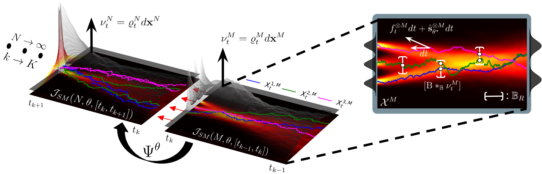
Figure 2: Illustrative Overview of Denoising MF-SDEs/WGFs. MF-SDEs governing $M$ particles are evolved with respect to vector fields $f_{t}^{\otimes M}+\mathbf{s}_{\theta}^{\otimes M}$ over the interval $[t_{k-1},t_{k}]$, interacting with proximate particles lying in $\mathbb{B}_{R}$. The illustration depicts the scenario in which the particle branching function $\Psi^{\theta}$ transforms the density of $M=3$ particles into an expanded density for $N=6$ particles $(\textit{e}.\textit{g}.,\text{branching ratio }\leavevmode\nobreak\ \mathfrak{b}=2)$ following the time interval $t_{k}$ and result in the joint density $\varrho_{t}^{N}$.

Our next step is to design an approximation framework that transforms the score-matching objective into computationally tractable variants. Let $\mathbb{N}=\{N_{k};N_{K}=N\}$ be a set of non-decreasing cardinality, and $\mathbb{T}=\{t_{k};t_{K}=T\}$ be a partition of the interval $[0,T]$, where $k\in\{0,\ldots,K\}$. Then, we subdivide Eq. 25 into $K$ sub-sequences to obtain alternative and computable upper-bounds:

Proposition 4.1.

(Subdivision) Under the assumption of reducibility and $\mathfrak{b}>0,N_{k+1}=\mathfrak{b}N_{k}$, the chaotic entropy can be split into $K$ sub-problems.

$$\mathcal{H}_{T}^{\infty}(\mu_{T})\precsim\lim_{K\rightarrow\infty}\sum_{k=0}^{K}\bigg{[}\sigma_{\zeta}^{-2}(T)\underbrace{\mathrm{E}(N_{k+1})}_{\text{Eq}.\leavevmode\nobreak\ \ref{eq:wasserstein_ve_1}}\\ +\frac{\mathcal{M}}{\sqrt{d}}\underbrace{\bigg{(}\frac{1}{{{\mathfrak{b}}}\sqrt{N_{k+1}}}\bigg{)}^{k}\mathcal{J}_{MF}(N_{k},\theta,\nu_{[t_{k},t_{k+1}]}^{N_{k}})}_{\text{Subdivision Errors }\geq\leavevmode\nobreak\ \mathcal{J}_{MF}^{N}(\theta,\nu_{[0,T]}^{N})}\bigg{]}.$$ (27)

We observe that chaotic entropy can be approximated by aggregating $K$ sub-problems of MF-SM, each corresponding to a unique cardinality $N_{k}$ and a specific interval $[t_{k},t_{k+1}]$. This implies that a divide-and-conquer strategy can be effectively employed to address problem $\mathbf{(P2)}$, by treating the sub-problems $\mathcal{J}_{MF}(N_{k},\cdot,\cdot)$ individually.

In the decomposed upper-bound in Eq. 27, the particle branching ratio $\mathfrak{b}$ moderates the impact of sub-problems for large cardinality in the score estimation, leading to improved robustness against $N$. Our final objective function in $\mathbf{(P3)}$ reflects the subdivision of chaotic entropy and the summation is only taken for finite $K$ sub-problems, leveraging the canceling effect gained from the branching ratio.

$$\mathbf{(P3)}\quad\min_{\theta}\sum_{N_{k}\in\mathbb{N}}^{K=|\mathbb{N}|}\frac{1}{\mathfrak{b}^{k}}\mathcal{J}_{MF}(N_{k},\theta,\nu_{[t_{k},t_{k+1}]}^{N_{k}}).$$ (28)

Section A.9.1 contains a detailed algorithmic procedures for training score networks $\mathbf{s}_{\theta}$ with the objective $\mathbf{(P3)}$.

Particle Branching Function $\Psi^{\theta}$. The discontinuity of $K$ piece-wise dWGFs $\{\nu_{t}^{N_{k}},t\in[t_{k},t_{k+1}]\}$ associated with individual sub-problems makes the sampling schemes intractable, necessitating the development of gluing pieces together to prevent abrupt changes in distribution. As a remedy, we introduce the particle branching function $\Psi_{N_{k+1}}^{\theta}$ to connect the end of previous segment of flows $(\textit{e}.\textit{g}.,\nu_{t_{k}}^{N_{k}})$ with the start of next flows $(\textit{e}.\textit{g}.,\nu_{t_{k}}^{N_{k+1}})$. In a distributional sense, this operation can be represented as a product with a push-forward measure:

$$(\underbrace{\mathbf{Id}^{\otimes\mathfrak{b}-1}}_{(\mathfrak{b}-1)N_{k}}\otimes\underbrace{\Psi^{\theta}}_{N_{k}})_{\#}\nu_{t_{k}}^{N_{k}}\leavevmode\nobreak\ \xlongrightarrow[]{}\leavevmode\nobreak\ \underbrace{\hat{\nu}_{t_{k}}^{\otimes\mathfrak{b}N_{k}}=\nu_{t_{k}}^{\mathfrak{b}N_{k}}}_{N_{k+1}=\mathfrak{b}N_{k}}.$$ (29)

where $(\cdot)_{\#}$ stands for the push-forward operator, and $\mathbf{Id}$ is a identity operator. As a consequence of particle branching, the intermediate flows of probability measure presented as a solution to dWGFs for $N_{k}$ particles $(\textit{i}.\textit{e}.,\nu_{t_{k}}^{N_{k}})$ is augmented with another $(\mathfrak{b}-1)N_{k}$ particles, yielding new flows with enhanced cardinality $N_{k+1}=\mathfrak{b}N_{k}$. Proposition A.8 reveals the explicit form of optimal particle branching.

Sampling Denoising Dynamics. After finishing training denoising MF-SDEs/WGFs with the triplet $(\mathbb{N},N,\mathfrak{b})$, we sample the chaotic dynamics by progressively increasing the cardinality in the middle of the denoising process. The procedure begins by taking initial Gaussian noises distributed as $\zeta_{T}^{\otimes N_{0}}$ and propagate particles via Euler scheme with score network $\mathbf{s}_{\theta}$ until reaching the next branching step at $T-t_{1}$ and each particle branches from $N_{0}$ to $\mathfrak{b}N_{0}=N_{1}$. By the iteration, we achieve the desired number of chaotic particles. Figure 2 provides an illustrative overview of the sampling procedure with particle branching along with the denoising WFGs. Section A.9.2 contains a detailed algorithmic procedure.

4.1 Mean-field Analysis of MF-CDMs

As this work primarily capitalizes on the mean-field property, this section aims to explore the theoretical implications and benefits of incorporating principles of PoC into the framework of SGMs. The subsequent theoretical findings provide insights to address the question (i.e., $\mathbf{Q1}$) posed earlier in Section 2.1.

Theorem 4.2.

(informal) Let $\mathfrak{f}\coloneqq\mathfrak{f}(\kappa)>0$ be a numerical constant dependent on log-Sobolev constant $\kappa$ with respect to proposed dWGFs. Given mild regularity conditions for $\mathbf{s}_{\theta}$, we have short-tailed concentration probability bound:

$$\mathbb{P}\left[\mathcal{H}(\nu_{t}^{M,N}|\mu_{t}^{\otimes M})\geq\varepsilon\right]\precsim\qquad(M\ll N\rightarrow\infty)\\ \mathcal{O}(\varepsilon^{-\varepsilon^{-d}})\cdot\mathcal{O}\left(\exp[-M\mathfrak{f}(\kappa)\varepsilon^{2}-M\mathfrak{f}(\kappa)\mathfrak{h}(R)]\right).$$ (30)

where For the numerical constant $\mathfrak{h}(R)$ dependent on the radius $R>0$ for truncation of convolution defined in Section A.3.

Concentration of Chaotic Entropy. The short-tailed concentration of chaotic entropy in Eq. 30 confirms that a relatively small number of particles $M$ suffices to reconstruct the mean-field surface $\mu_{t}$ even when the total cardinality diverges to infinite $(N\rightarrow\infty)$. In addition, it demonstrates that infinite cardinality constraints $(\textit{i}.\textit{e}.,\lim_{N\rightarrow\infty})$ specified in $\mathbf{(P2)}$ can be circumvented by subdivision of chaotic entropy in $\mathbf{(P3)}$, as score estimation errors are tolerable in practice with a finite number of sub-problems $|\mathbb{N}|<\infty$ and particle counts $\{N_{k}\}_{k\leq K}$.

Theorem 4.3.

(informal) Let us define $F_{t}\coloneqq\norm{\mathcal{G}_{t}}_{E}^{2}+\norm{\nabla\mathcal{G}_{t}}_{F}^{2}$, and $\mathbb{E}_{\nu_{[0,T]}^{N}}\mathbb{E}_{t\sim p(t)}F_{t}(\mathbf{X}_{t}^{N})=\mathcal{J}_{MF}^{N}(\theta,\nu_{[0,T]}^{N})$, there exist constants $\mathrm{C}_{5},\mathrm{C}_{6}>0$, $\mathbb{N}^{+}\ni q>4$ such that

$$\mathbb{P}\left(\left|\mathbb{E}_{t}F(\mathbf{X}_{t}^{N})-\mathcal{J}_{MF}(N=1,\theta,\mu_{[0,T]})\right|\geq\varepsilon\right)\leq$$ (31)

$$\exp(-\mathrm{C}_{5}\mathfrak{f}(\kappa)^{-2}\left[\varepsilon\sqrt{N}-\mathrm{C}_{6}\sqrt{\left(1+N^{(-q+4)/2q}\right)}\right]^{2}).$$

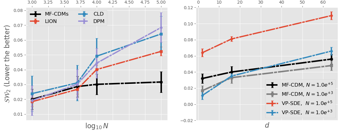
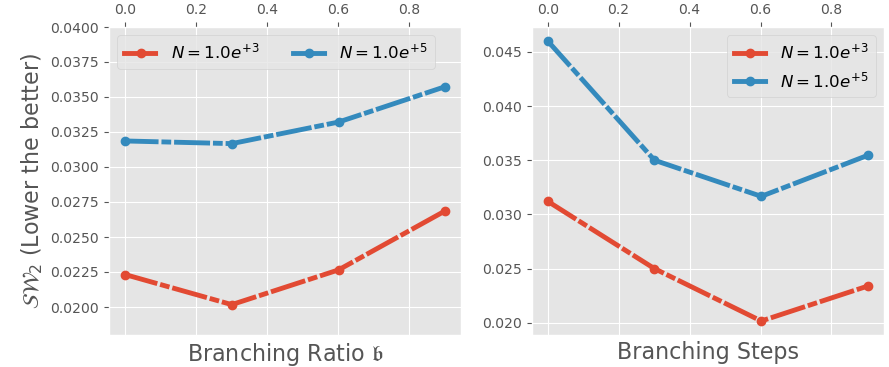
Figure 3: (Left) Scalability to Data Complexity. Performance comparisons with varying data dimensionality $d$ and cardinality $N$. (Right) Ablation Study on Hyperparameters. Performance variation of MF-CDMs with respect to different hyperparameters; branching ratio $b\in\{1,2,4,8\}$ and number of particle branching $|\mathbb{K}^{\prime}|\in\{1,2,4,8\}$.

Concentration of MF-SM. Our second observation in Eq. 31 elucidates that our MF-SM is naturally concentrated on their mean-field limit $\mu_{t}$ with asymptotically stable probability upper bounds. This shows the remarkable robustness of our objective function when $N\rightarrow\infty$, where conventional score matching objectives $\mathcal{J}_{SM}$ in Eq. 4 are highly vulnerable to this extreme condition because of the absence of guaranteed stability, as illustrated by Eq.31.

5 Related Works

Mean-field Dynamics in Generative Models. Modeling score-based generative models via population dynamics (Koshizuka & Sato, 2023; Chen et al., 2021; Shi et al., 2023) have gained attention recently. Among these, mean-field dynamics through a particle interaction was explored in (Liu et al., 2022), where the Schrödinger bridge was integrated to handle mean-field games for the approximation of large population data distributions. (Lu et al., 2023) derived score transportation directly from the mean-field Fokker-Planck equation where particle interaction was derived for score-based learning. While these works primarily focus on an analytic perspective and assume an infinite dimensional setting associated with high-dimensional PDEs, our method adopts PoC as a limit algorithm to reduce the potential complexity encountered in dealing with PDEs.

Diffusion Models for Unstructured Data. Recent studies have demonstrated the exceptional performance of diffusion dynamics in point-cloud synthesis (Luo & Hu, 2021; Zhou et al., 2021; Zeng et al., 2022; Tyszkiewicz et al., 2023), with a focus on architectural design to impose structural constraints on unstructured data formats. Another stream of research (Hoogeboom et al., 2022; Xu et al., 2023) considered global geometric constraints to capitalize on equivariance property in the modeling of point-clouds. Despite their superior performance, the aforementioned methods face a limitation in the maximum capacity of cardinality owing to rigid structural constraints on localization. In contrast, our method employs a flexible localization using mean-field interaction, requiring only a weak probabilistic structure over the particle set but consistently assures robust performance.

6 Empirical Study

This section provides a numerical validation of the efficacy of integrating MFT into the SGM framework, particularly in extreme scenarios of large cardinality, where previous works struggle to achieve robust performance.

Benchmarks. We compare our MF-CDMs with well-recognized models in score-based generative models: VP-SDE (Song et al., 2021c), CLD (Dockhorn et al., 2022), and diffusion models for 3D point-cloud: DPM (Luo & Hu, 2021), LION (Zeng et al., 2022), PVD (Zhou et al., 2021). For information on the implementation of score networks along with hyperparameters and statistics of datasets with pre-processing, please refer to Sec A.9.

6.1 Synthetic Dataset: Robustness Analysis

Method	$\small(10^{3},5)$	$(10^{3},32)$	$(10^{5},5)$	$(10^{5},32)$
VP-SDEs	$2.198$	$2.683$	$6.943$	$7.542$
CLD	$2.387$	$2.826$	$6.411$	$7.131$
DPM	$1.924$	$2.007$	$6.847$	$7.448$
LION	$\mathbf{1.841}$	$\mathbf{1.919}$	$5.234$	$6.105$
MF-CDMs	$2.017$	$2.413$	$\mathbf{3.167}$	$\mathbf{4.059}$

Table 2: Performance Evaluation on the Synthetic data. We measure performance across different data complexities $(N,d)$ by applying the sliced $2$-Wasserstein distance scaled by a factor of $\times 10^{2}$. The best results are highlighted in bold.

The first experiment is designed to evaluate the impact of dimensionality ($\textit{i}.\textit{e}.,d$) and cardinality ($\textit{i}.\textit{e}.,N$) on the robustness of benchmark SGMs when dealing with unstructured data. For this purpose, we generate a synthetic dataset with an equi-weighted Gaussian mixture $\{\mathbf{Y}_{n}\}_{n}^{N}\sim\mathbf{GMM}^{d}(d\mathbf{x}^{d})\coloneqq(1/8)\sum^{8}_{a}\mathcal{N}[\mathbf{m}_{a},\sigma_{a}\mathbf{I}_{d}]$ where Gaussian parameters $(\mathbf{m}_{a},\sigma_{a})$ are randomly selected within unit-cubes $[-1,1]^{d}$. The challenge arises as all elements $\{\mathbf{Y}_{n}\}$ satisfies $p(\mathbf{Y}_{m})=p(\mathbf{Y}_{n})$ for any $m\neq n\leq N$, and this interchangeability complicates to extract meaningful local associations among the elements, which is essential for efficient learning. To evaluate performance, we employ a tool from optimal transport, sliced 2-Wasserstein distance (i.e., $\mathcal{SW}_{2}$) (Kolouri et al., 2019), known for its efficiency in capturing discrepancies between unstructured data instances, especially at high cardinality.

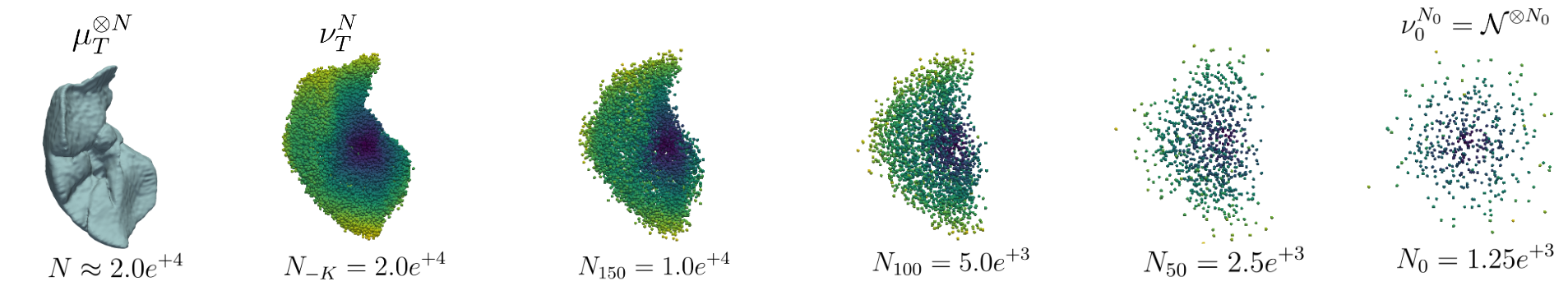
Figure 4: Qualitative Results on MedShapeNet Dataset. Both $\mu_{T}^{\otimes N}$ and $\nu_{T}^{N_{-K}}$ illustrate the target and generated 3D shapes, where displayed liver object in MedShapeNet dataset comprises a high-cardinality point-set of nearly $2.0E^{+4}$ points.

Results. Fig 3 and Table 2 present qualitative results when the set cardinality and dimensionality change within the ranges of $N\in\{10^{3},10^{5}\}$ and $d\in\{5,32\}$. We note that other methods can easily surpass ours, as the proposed mean-field modeling loses its strength and entails excessive computational complexity with small cardinality (i.e., , $N=10^{3}$). While existing methods show promising results in low cardinality experiments, their performance significantly deteriorates under conditions of extreme cardinality (i.e., , $N=10^{5}$). The reason for performance decline is due to their shortcomings in the explainable analysis regarding the curse of dimensionality issue and thus lack of effective modeling of inter-associations among elements.

In comparison with benchmarks, our method demonstrates robust performance, significantly outperforming all other benchmarks by a large margin in scenarios of $N=10^{5}$. Since our methodology has extended VP-SDEs through the integration of PoC in reverse dynamics, the performance gain of MF-CDM over VP-SDEs implies that the chaotic modeling significantly enhances the robustness of conventional SGMs.

	ShapeNet	MedShapeNet
Methods	EMD $\downarrow$   /   CD $\downarrow$	EMD $\downarrow$   /   CD $\downarrow$
VP-SDEs	$4.860\leavevmode\nobreak\ \leavevmode\nobreak\ /\leavevmode\nobreak\ \leavevmode\nobreak\ 4.585$	$6.387\leavevmode\nobreak\ \leavevmode\nobreak\ /\leavevmode\nobreak\ \leavevmode\nobreak\ 4.616$
CLD	$4.083\leavevmode\nobreak\ \leavevmode\nobreak\ /\leavevmode\nobreak\ \leavevmode\nobreak\ 5.865$	$8.647\leavevmode\nobreak\ \leavevmode\nobreak\ /\leavevmode\nobreak\ \leavevmode\nobreak\ 5.632$
DPM	$3.058\leavevmode\nobreak\ \leavevmode\nobreak\ /\leavevmode\nobreak\ \leavevmode\nobreak\ 3.269$	$6.139\leavevmode\nobreak\ \leavevmode\nobreak\ /\leavevmode\nobreak\ \leavevmode\nobreak\ 3.248$
PVD	$3.445\leavevmode\nobreak\ \leavevmode\nobreak\ /\leavevmode\nobreak\ \leavevmode\nobreak\ 3.032$	$6.386\leavevmode\nobreak\ \leavevmode\nobreak\ /\leavevmode\nobreak\ \leavevmode\nobreak\ 5.902$
LION	$3.248\leavevmode\nobreak\ \leavevmode\nobreak\ /\leavevmode\nobreak\ \leavevmode\nobreak\ 3.248$	$6.221\leavevmode\nobreak\ \leavevmode\nobreak\ /\leavevmode\nobreak\ \leavevmode\nobreak\ 5.135$
MF-CDMs	$\mathbf{2.627\leavevmode\nobreak\ \leavevmode\nobreak\ /\leavevmode\nobreak\ \leavevmode\nobreak\ 1.877}$	$\mathbf{4.046\leavevmode\nobreak\ \leavevmode\nobreak\ /\leavevmode\nobreak\ \leavevmode\nobreak\ 2.764}$

Table 3: Performance Evaluation of 3D point-cloud generation on ShapeNet/MedShapeNet datasets. The best results are highlighted in bold. Evaluation metrics on EMD and CD are scaled by $10^{2}$ and $10^{2}$, respectively.

6.2 Real-world Dataset: 3D Point-cloud Generation

In the second experiment, we benchmark the empirical performance of MF-CDMs along with existing SGMs for 3D shape diffusion models on two datasets: ShapeNet (Chang et al., 2015) and MedShapeNet (Li et al., 2023), with each 3D point-clouds instance consisting of $\mathbf{N=1.0E^{+4}}$ and $\mathbf{N=2.0E^{+4}}$ points, respectively. The data cardinality in our experiments is up to $10$ times larger than standard setups, which typically focus on scenarios with a relatively limited number of points, ($\textit{e}.\textit{g}.,2048$). For the fair comparison, we utilized evaluation metrics suggested in (Yang et al., 2019) to compare benchmarks (i.e., MMD-EMD, MMD-CD). Owing to the numerical instability of these metrics when applied to high-cardinality objects, we randomly sub-sampled $2048$ points from both the generated $\nu_{T}^{N}$ and the target $\mu_{T}^{\otimes N}$ objects and performed numerical comparisons.

Results. Table 3 summarizes performance comparisons with benchmarks. Without requiring any strong localization modules, our MF-CDM surpasses all other benchmarks on two datasets, showing its efficiency in real-world settings. It is worth highlighting that task-oriented methods, such as PVD and LION, have achieved state-of-the-art performance on the ShapeNet dataset with $2048$ points. However, they suffer from a drastic performance decline when applied to the MedShapeNet dataset as they depend on fixed localization modules, which are primarily optimized for low cardinality data. We also posit that our superiority stems from the concentration property of large particle systems, as supported by our theoretical findings in Section 4.1.

Figure 4 provides a visualization of the intermediate 3D shape during the denoising process with dWGFs. The simulation of dWGFs starts with $N_{0}=1.25e^{+3}$ particles and the number of particles are doubled $(\textit{e}.\textit{g}.,b=2)$ at each of the branching steps $k\in\{50,100,150,200\}$, reaching $N\coloneqq N_{-K}=2.0e^{+4}$ at the end of the process. The final illustrative result, $\nu_{T}^{N_{-K}}$, closely resembles the target 3D anatomic structure $\mu_{T}^{\otimes N}$ $(\textit{i}.\textit{e}.,\textit{liver})$.

7 Conclusion

In this study, we propose MF-CDMs, a novel class of SGMs designed for the efficient generation of unstructured data instances with infinite dimensionality. Beginning with the original entropy minimization problem $\mathbf{(P0)}$, we gradually enlarge our discussion to leverage principles of MFT and pose advanced problems $\mathbf{(P1)}\sim\mathbf{(P3)}$ to deal with the curse of dimensionality issues. Our theoretical results reveal that the MF-CDMs naturally inherit chaoticity, ensuring the robust behavior of our model with infinite cardinality. Experimental results on both synthetic and 3D shape datasets empirically validate the superior capability of our framework in generating data instances. In future works, we hope to apply our methodology across diverse tasks in scientific domains, such as physical simulation of large-particle dynamical system (Karniadakis et al., 2021), large-molecule polymer generation (Anstine & Isayev, 2023).

Impact Statement

This paper presents work whose goal is to advance the field of Machine Learning. There are many potential societal consequences of our work, none which we feel must be specifically highlighted here.

Appendix A Appendix

A.1 Notations

Throughout the paper, we adhere to the following notations:

• Without loss of generality, we employ the same notation for the tensor product across different objects, including functions, and probability measures denoted as $f\otimes g$, $\mu\otimes\nu$. • For any member of continuous bounded and integrable function class $f$, we denote the self $N$-products and its integral as $$f^{\otimes N}(\mathbf{x}^{N})=[f(\mathbf{x}_{1}),\cdots f(\mathbf{x}_{N})],\quad\int f^{\otimes N}(\mathbf{x}^{N})\mu^{\otimes N}(d\mathbf{x}^{N})=\prod_{i\leq N}\int f(\mathbf{x}_{i})\mu(\mathbf{x}_{i}),$$ (32) • We denote coordinate system of for $N$-particle system as $\mathbf{x}^{N}=(\mathbf{x}_{1},\cdots\mathbf{x}_{N})\in\mathcal{X}^{N}$ where each component is represented as $\mathbf{x}_{i}\in\mathcal{X}$, $i\leq N$. • For the probability measure $\nu$ and the integrable test function $f$, we simply denote $\langle\nu,f\rangle\coloneqq\int fd\nu$ as integral. • The law of the $N$-particle joint density, $\nu_{t}^{N}$, falls within the 2-Wasserstein space, which specifically contains absolutely continuous measures, represented by $\mathcal{P}_{2}\equiv\mathcal{P}_{2,ac}$. We routinely presume the absolute continuity of all probability measures in this context. • The $N$-particle mean-field dynamics is represented as $\mathbf{X}^{N}\sim\nu^{N}\in\mathcal{P}_{2,ac}(\mathcal{X}^{N})$. Following by the absolutely continuity, we define the density representation with Radon-Nikodym derivative: $d\nu^{N}=\varrho^{N}d\mathbf{x}^{N}$. • The first $M$ component of $N$-particles will be denoted by $\mathbf{X}^{M,N}\sim\nu^{M,N}\in\mathcal{P}_{2,ac}(\mathcal{X}^{M})$ with $d\nu^{M,N}=\varrho^{M,N}d\mathbf{x}^{M}$. • The $N$-product of probability measure $\nu$ will be denoted by $\nu^{\otimes N}\in\mathcal{P}_{2,ac}(\mathcal{X}^{N})$ with $d\nu^{\otimes N}=\varrho^{\otimes N}d\mathbf{x}^{N}$. • The Euclidean and Frobenius norm will be denoted by $\norm{a}_{E},\norm{A}_{F}$, respectively. • $\mathbf{Sym}(d)$, Set of symmetric matrices with size $(d\times d)$; $\mathbf{GL}(d)$, general liner matrix group of size $(d\times d)$. • Within our mathematical context, the symbols are defined as follows: $D$ and $D_{\varrho}$ for abstract and functional derivatives, respectively; $\nabla_{x}\coloneqq\nabla$ for the Euclidean gradient; $\nabla_{\mathcal{P}_{2}}$ for the Wasserstein gradient; and $\partial_{t}$ for the temporal derivative. For simplicity, the Jacobian matrix of vector-valued objects $h$ will be interchangeably denoted by $\nabla h\coloneqq\mathcal{J}h$. • In the paper, $\mathcal{G}_{t}$ represents the deviation of score functions for an $N$-particle system, $\mathcal{G}_{t}^{i,N}$ denotes the projection of these functions onto the $i$-th component, and $\mathcal{G}_{t}^{\infty}$ corresponds to its mean-field limit. • $\mathcal{L}_{p}(\mathcal{X}),$ denotes the $L_{p}$ function space on $\mathcal{X}$, • $\mathbf{Lip}(f)$ is a Lipschitz constant of continuous and bounded function $f$. • $\mathbb{N}$ denotes the index set for cardinality, and $\mathbb{N}^{+}$ is defined as a set of positive integers. • For the maximum and minimum of two real-values, we follow the convention for the notation in literature as $\max(a,b)=a\wedge b,\min(a,b)=a\vee b$.

A.2 Assumptions and Lemmas

We establish the following assumptions to facilitate existing theoretical frameworks of MFT in analyzing the behavior of the proposed MF-SDEs/dWGFs.

1. $\mathbf{(H1)}.$ We always assume the large cardinality in data representation, $\textit{i}.\textit{e}.,N\gg d$. 2. $\mathbf{(H2)}.$ For all $j\leq N$, $\mathrm{A}$ and the mean-field interaction $\mathrm{B}$ satisfy the Lipschitz continuity with respect to both $\mathcal{X}$ and $\mathcal{P}_{2,ac}$, $\displaystyle\norm{[\mathrm{B}*\nu](\mathbf{x}^{j})-[\mathrm{B}*\nu^{\prime}](\mathbf{y}^{j})}_{E}^{2}\leq\mathrm{C}_{\mathrm{B}}\left(\norm{\mathbf{x}^{j}-\mathbf{y}^{j}}_{E}^{2}+\mathcal{W}_{2}^{2}(\nu,\nu^{\prime})\right),$ (33) $\displaystyle\norm{A(s,\mathbf{x}^{j})-A(t,\mathbf{y}^{j})}_{E}^{2}\leq\mathrm{C}_{\mathrm{A}}\norm{\mathbf{x}^{j}-\mathbf{y}^{j}}_{E}^{2}+\mathrm{C}_{A}(s\wedge t-s\vee t)^{2}.$ (34) By definition and assumptions above, the Lipschitz continuity for the score networks is naturally inferred as $$\norm{\mathbf{s}_{\theta}(s,\mathbf{x}^{j},\nu)-\mathbf{s}_{\theta}(t,\mathbf{y}^{j},\nu^{\prime})}_{E}^{2}\leq 2(\mathrm{C}_{\mathrm{A}}\wedge\mathrm{C}_{\mathrm{B}})\norm{\mathbf{x}^{j}-\mathbf{y}^{j}}_{E}^{2}+\mathrm{C}_{A}(s\wedge t-s\vee t)^{2}+\mathrm{C}_{\mathrm{B}}\mathcal{W}_{2}^{2}(\nu,\nu^{\prime}).$$ (35) We assume that the second moment of proposed score networks is bounded. $$\norm{\mathbf{s}_{\theta}(t,\mathbf{x}^{j},\nu)}_{E}^{2}\leq\mathrm{D}(1+\norm{\mathbf{x}^{j}}_{E}^{2}).$$ (36) 3. $\mathbf{(H3)}.$ There exist real-valued functions $\mathbf{A},\mathbf{B}\in C^{2}(\mathcal{X})$ and $\mathbf{A}^{N},\mathbf{B}^{N}\in C^{2}(\mathcal{X}^{N})$ such that $$\nabla\mathbf{A}=\mathrm{A},\leavevmode\nobreak\ \nabla\mathbf{A}^{N}=\mathrm{A}^{N},\quad\nabla\mathbf{B}=\mathrm{B},\leavevmode\nobreak\ \nabla\mathbf{B}^{N}=\mathrm{B}^{N},$$ (37) and those functions are uniformly convex. Equivalently, there exist constants $\gamma_{\mathrm{A}},\gamma_{\mathrm{B}},\gamma_{\mathrm{B}}^{\prime}>0$ such that Hessian matrices satisfy following: $$\nabla^{2}\mathbf{A}\succeq\gamma_{\mathrm{A}}\mathbf{I}_{d},\quad\gamma_{\mathrm{B}}^{\prime}\mathbf{I}_{d}\succeq\nabla^{2}\mathrm{B}\succeq\gamma_{\mathrm{B}}\mathbf{I}_{d}.$$ (38) 4. $\mathbf{(H4)}.$ Almost surely, we can always find the score networks $\theta\in\Theta$ that can replace the score function of MF-SDEs. $$\mathbb{P}\left[\mathbf{s}_{\theta}(t,\mathbf{x}^{N},\nu_{t}^{N})=\nabla\log\varrho_{t}^{N}(\mathbf{x}^{N})\right]=1,\quad\leavevmode\nobreak\ \forall N\in\mathbb{N}.$$ (39) 5. $\mathbf{(H5)}.$ For any $t\in[0,T]$, there exist a constant $q>2,q\neq 4$, such that the solution to non-linear Fokker-Planck equation $\mu_{t}$ has finite $q$-th moment, $\textit{i}.\textit{e}.,\left(\mathbb{E}_{\mu_{t}}[\norm{\mathbf{x}}^{q}]\right)^{1/q}<\infty$. 6. $\mathbf{(H6)}.$ For some constant $a>0$, the following numeric estimation are bounded for any $1\leq M\leq N$: $$\mathbb{E}_{\mathbf{x}\sim\nu_{t}^{M,N}}\exp(a||\mathbf{x}||_{E}^{2})<\infty,\leavevmode\nobreak\ \quad\forall\nu_{t}^{M,N}(d\mathbf{x}^{M})=\varrho_{t}^{M,N}(\mathbf{x}^{M})d\mathbf{x}^{M}.$$ (40)

Lemma A.1.

(Grönwall’s Lemma, Theorem 5.1 (Ethier & Kurtz, 2009)). Assume $h:[0,T]\rightarrow\mathbb{R}$ is bounded non-negative measurable function on $[0,T]$ and $g:[0,T]\rightarrow\mathbb{R}$ is a non-negative integrable function. Let following inequality holds for the constant $\mathrm{a}>0$, $$h(t)\leq B+\int_{0}^{t}g(s)h(s)ds,\quad\longrightarrow\quad h(t)\leq B\exp(\int_{0}^{t}g(s)ds),\qquad t\in[0,T].$$ (41)

A.3 Exchangeability, Chaocity, Reducibility

In this section, we discuss three core properties (eg, exchangeability, chaocity, reducibility) of the proposed mean-field $N$-particle system, which will be often referenced in subsequent proofs.

Exchangeability. We first show the universal exchangeability property of sample particles:

Proposition A.2.

(Exchangebility of $N$-particle system.) Let $\mathbf{X}_{t}^{N}\sim\nu_{t}^{N}$ be a solution to mean-field SDEs defined in Eq. 6. Assume that $\mathbf{X}_{0}^{N}\sim\mathcal{N}^{\otimes N}[\mathbf{I}_{d}]$. Then, any particles $\{\mathbf{X}_{t}^{i,N}\}_{i\leq N}$ at any time $t\in(0,T]$ are exchangeable.

Proof.

Since the infinitesimal generator for $N$-particle system lies in the set $\mathcal{L}^{N}_{t}\in\{\mathcal{L};\tau^{-1}\mathcal{L}\tau=\mathcal{L},\leavevmode\nobreak\ \tau\in S_{N}\}$, all the solutions $\varrho_{t}^{N}$ (or $\nu_{t}^{N}$) to the Liouville equation in Eq. 18 are trivially symmetric measures at any time $t\in(0,T]$ when the initial state $\varrho_{0}^{N}$ (or $\nu_{0}^{N}$) is symmetric. The initial constraint $\varrho_{0}^{N}=\mathcal{N}^{\otimes N}$ ensures exchangeability of a set of initial states since samples drawn from two projected components $\pi_{i}^{N}\mathcal{N}^{\otimes N}$ and $\pi_{j}^{N}\mathcal{N}^{\otimes N}$ are i.i.d for any pairs $(i,j)\in\mathbb{N}^{+}\oplus\mathbb{N}^{+}$, meaning that those random variables are exchangeable. ∎

The rationale behind the equality in Eq. 9 is based on the result of Proposition A.2, since the initial state of the denoising process assumes i.i.d Gaussianity with the fact that its associated generator $\mathcal{L}^{N}_{t}$ is concurrently acting on every particles.

Design of Score Networks, $\mathrm{A}_{\theta}$, $[\mathrm{B}_{\theta}*_{\mathbb{B}}\nu_{t}^{N}]$. We first consider the equi-weighted $N$-product of score networks as following.

$$\mathrm{A}_{\theta}(t,\mathbf{x}^{N})=\hat{\mathrm{A}}^{\otimes N}_{\theta}(t,\mathbf{x}^{N})=\frac{1}{\sqrt{N}}[\mathrm{A}(t,\mathbf{x}_{1},\theta),\cdots,\mathrm{A}(t,\mathbf{x}_{N},\theta)]^{T}\in\mathcal{X}^{N}.$$ (42)

Note that $\mathbf{Lip}(\hat{\mathrm{A}}^{\otimes N})=\sum_{j}^{N}\mathbf{Lip}(\hat{\mathrm{A}}_{j}^{\otimes N})=\mathbf{Lip}(\mathrm{A}_{\theta})$. Consequently, we define truncated convolution for $N$-particle system as

$$[\mathrm{B}_{\theta}*_{\mathbb{B}}\nu_{t}^{N}](\mathbf{x}^{N})=\frac{1}{\sqrt{N}}[[\mathrm{B}_{\theta}*\hat{\nu}_{t}^{N}](\mathbf{x}_{1}),\cdots,[\mathrm{B}_{\theta}*\hat{\nu}_{t}^{N}](\mathbf{x}_{N})]^{T},$$ (43)

where $\hat{\nu}_{t}^{N}=(1/N)\sum_{i^{\prime}}^{N}\mathbf{X}_{t}^{i^{\prime},N}$ is an empirical projection of $\nu_{t}^{N}\in\mathcal{P}_{2}(\mathcal{X}^{N})$ onto $\hat{\nu}_{t}^{N}\in\mathcal{P}(\mathcal{P}_{2}(\mathcal{X}))$. Then, each component in Eq. 43 can be represented as

$$[\mathrm{B}_{\theta}*_{\mathbb{B}}\hat{\nu}_{t}^{N}](\mathbf{x}_{j})=\int\mathrm{B}_{\theta}(\mathbf{x}_{j}-\mathbf{y}_{j})d\nu_{t}^{R}[\mathbf{x}_{j}](\mathbf{y}_{j}),\quad 1\leq j\leq N,$$ (44)

where $\mathrm{B}_{\theta}:\mathbb{R}^{d}\rightarrow\mathbb{R}^{d}$ are score networks parameterized by $\theta\in\Theta$. Here, the truncated measure $\nu_{t}^{R}[\mathbf{x}_{j}](\mathbf{y}_{j})$ with respect to the centered particle $\mathbf{x}_{j}\in\mathbb{R}^{d}$ is defined as

$$\quad d\nu_{t}^{R}[\mathbf{x}_{j}](\mathbf{y}_{j})=\frac{\chi_{\mathbb{B}_{R}^{\mathbf{x}_{j}}}\hat{\nu}_{t}^{N}(d\mathbf{y}_{j})}{\hat{\nu}_{t}^{N}[\mathbb{B}_{R}^{\mathbf{x}_{j}}]},$$ (45)

where $\mathbb{B}_{R}^{\mathbf{x}_{j}}$ is a Euclidean ball of radius $R$ centered at $\mathbf{x}_{j}$ and $\chi_{A}$ represents an indicator function defined on any set $A\subseteq\mathbb{R}^{d}$.

Reducibility. We say that the function $h:\mathcal{X}^{N}\rightarrow\mathcal{X}^{N}$ is reducible if there exists at least one $\mathcal{X}$-valued function $\hat{h}:[0,T]\times\mathcal{X}\rightarrow\mathcal{X}$ such that $h=\hat{h}^{\otimes N}$ uniformly, where the function product $\hat{h}^{\otimes N}(t,\mathbf{x}^{N})\in\mathcal{X}^{N}$ is defined in Eq. 32. With the definition, the notion of reducibility can be formalized as a kernel of the following functional $\mathcal{R}$ on Sobolev space:

$$\mathcal{R}(h)\coloneqq\inf_{\hat{h}\in W^{1,2}}\left[\norm{h(t,\mathbf{x}^{N})-\hat{h}^{\otimes N}(t,\mathbf{x}^{N})}_{W}\right].$$ (46)

Any functions $h$ in the kernel of functional $\textit{i}.\textit{e}.,\mathbf{Ker}(\mathcal{R})=\{h;\mathcal{R}(h)=0,h\in W^{1,2}(\mathcal{X}^{N})\}$ operates in a particle-wise manner, acting on each particle in parallel.

By the direct calculation, one can show that our score networks $(\textit{i}.\textit{e}.,\mathbf{s}_{\theta}\coloneqq\mathrm{A}_{\theta}+[\mathrm{B}_{\theta}*_{\mathbb{B}}\nu_{t}^{N}])$ are reducible and ready to be implemented for our purpose, as Proposition A.3 assures the chaoscity. Furthermore, one can easily show that vector fields $\nabla V^{N}$ of mean-field VP-SDE in 17 also satisfy reducibility. The reducibility condition, particularly, results in substantial computational efficiency in the modeling of score networks $\mathrm{A}_{\theta},\mathrm{B}_{\theta}\in\mathbf{Ker}(\mathcal{R})$. It permits point-wise operation through GPU-based calculations, thus accelerating the sampling process of the $N$-particle system in high cardinality environments. The reducibility property is critical in our approach, ensuring the particles’ chaotic behavior and scalability in the practical application of numerical implementation.

Chaocity. We conclusively demonstrate that our $N$-particle system, modeled by MF-SDEs, not only achieves $\mu_{T}$-chaos but also exhibits stability in its limit behavior.

Proposition A.3.

(Equivalence) Assuming mild Lipschitz continuity, the following three statements are equivalent: 1. The $N$-particle entropy Eq. 11 becomes chaotic if score networks $\mathbf{s}_{\theta}$ are reducible. 2. A joint probability density $\varrho_{T}^{N}$ solving the Liouville equation in Eq. 18 is $\mu_{T}$-chaotic. 3. The solution to the dWGF for $N$-particle system in Eq. 18 becomes $\mu_{t}$-chaotic if score networks $\mathbf{s}_{\theta}$ are reducible.

Proof.

The classical result of the propagation of chaos (Jabin & Wang, 2017) with the Lipschitz continuity assumption in $\mathbf{(H2)}$ assures that the denoising dynamics with reducible score networks induce chaoscity as exchangeability is already satisfied by the result of Prop A.2. Following by the result suggested in Theorem 1.4 (Hauray & Mischler, 2014), Kac’s chaos $(\textit{i}.\textit{e}.,\mu_{T}=\lim_{N\rightarrow\infty}\nu_{T}^{N})$ identically implies chaotic entropy given by assumptions of Lipschitz continuity. ∎

A.4 Wasserstein Variation Equation

Gradient flows on $\mathcal{P}_{2,ac}$, Itô’s flows of Measures. With mild assumptions on the regularity of energy functionals (e.g., functional differentiability), Wasserstein gradient can be identified with Lions’ $L$-derivative (Cardaliaguet, 2010) by utilizing Gâteaux (or Fréchet) derivative of semi-martingale lifting. To be more specific, Theorem A.4 reveals the fundamental structure that Eq. 50 can be rewritten in an alternative form based on a functional analytic perspective.

Theorem A.4.

(Carmona et al., 2018) Let us assume that functional $\mathcal{E}$ has a first variation $\partial\mathcal{E}/\partial\delta|_{\mu}$ for any $\mu\in\mathcal{K}\subset\mathcal{P}_{2,ac}$, and define spatial gradient of first variation as $$\mathcal{P}_{2,ac}\times\mathbb{R}^{d}\ni(\mu,\mathbf{x})\mapsto\nabla_{x}\frac{\partial\mathcal{E}}{\partial\delta}[\mu](\mathbf{x})\in\mathbb{R}^{d}.$$ (47) Assume that the mapping is jointly continuous in $(\mu,\mathbf{x})$, and well-defined, at most of the linear growth in $\mathbb{R}^{d}$, uniformly bounded in subset $\mathcal{K}\subset\mathcal{P}_{2,ac}$. Then Lions’ $L$-derivative is identical to the spatial gradient of the first variation.

For the a test function $\varphi$ and a solution $\varrho_{t}$ to dWGFs for $N\rightarrow\infty$ (e.g., McKean-Vlasov equation), we apply Gateaux derivative to the infinite-dimensional energy functional $\mathcal{E}:[0,T]\times\mathcal{L}_{2}(\mathcal{X})\rightarrow\mathbb{R}$,

$$\begin{split}\mathcal{E}(t,\varrho_{t})&=\int D_{\varrho}\mathcal{E}(t,\varrho_{t},\mathbf{x})\frac{\partial}{\partial t}\varrho_{t}d\mathbf{x}dt\\ &=\mathbb{E}\left[\nabla_{x}D_{\varrho}\mathcal{E}(t,\varrho_{t},\mathbf{x})\cdot\nabla V(t,\mathbf{x},\nu_{t})+\frac{1}{2}\mathbf{Tr}[\Sigma(t,\mathbf{x})\Sigma(t,\mathbf{x})^{T}\nabla_{x}^{2}D_{\varrho}\mathcal{E}(t,\varrho_{t},\mathbf{x})]\right]dt,\end{split}$$ (48)

A variety notions for the derivatives of Equation 48 have been explored in the literature (Guo et al., 2023; Carmona et al., 2018; Dos Reis & Platonov, 2023; Santambrogio, 2015). We examine the identity and details among them as follows:

$$\nabla_{x}D_{\varrho}\mathcal{E}|_{t,\mathbf{x},\varrho=\varrho_{t}}\leavevmode\nobreak\ \leavevmode\nobreak\ \xleftrightarrow{\leavevmode\nobreak\ \leavevmode\nobreak\ \text{Sec\leavevmode\nobreak\ 7.2\leavevmode\nobreak\ }\text{\cite[citep]{(\@@bibref{AuthorsPhrase1Year}{santambrogio2015optimal}{\@@citephrase{, }}{})}}\leavevmode\nobreak\ \leavevmode\nobreak\ }\leavevmode\nobreak\ \leavevmode\nobreak\ \nabla_{x}\frac{\partial\mathcal{E}}{\partial\delta}|_{t,\mathbf{x},\varrho_{t}}\leavevmode\nobreak\ \leavevmode\nobreak\ \xleftrightarrow{\leavevmode\nobreak\ \text{Theorem\leavevmode\nobreak\ \ref{theorem:appendix_equivalance}}\leavevmode\nobreak\ }\leavevmode\nobreak\ \leavevmode\nobreak\ \nabla_{\mathcal{P}_{2}}\mathcal{E}|_{t,\mathbf{x},\varrho_{t}}.$$ (49)

Assuming the appropriate regularity conditions for each energy functional, we find that three distinct notions of derivatives in Eq 49 are congruent. This observation leads us to delve into an alternative definition of the functional derivative and examine its role in defining the evolution of measures over time.

Definition A.5.

(Itô’s Flows of Measures) Given semi-martingale $\mathbf{X}_{(\cdot)}$ with finite variation $\mathbb{E}[\textbf{Var}(V)]<\infty$ and finite quadratic variation $\mathbb{E}[d[\mathbf{X}_{(\cdot)},\mathbf{X}_{(\cdot)}]]<\infty$, the time-varying energy functional $\mathcal{E}:[0,T]\times\mathcal{P}_{2,ac}\rightarrow\mathbb{R},\leavevmode\nobreak\ \mathcal{E}\in\mathcal{C}^{1,1}(\mathcal{P}_{2}(\mathcal{X}))$ associated with differential calculus on the Wasserstein space $\mathcal{P}_{2,ac}$ evolves according to dynamics defined as: $$d\mathcal{E}(t,\mathbf{Law}(\mathbf{X}_{t}))=\mathbb{E}\left[\nabla_{x}\frac{\partial\mathcal{E}}{\partial\delta}(t,\mathbf{Law}(\mathbf{X}_{t}))\cdot d\mathbf{X}_{t}\right]+\mathbb{E}\left[\frac{1}{2}\mathbf{Tr}\left(\nabla_{x}^{2}\frac{\partial\mathcal{E}}{\partial\delta}(t,\mathbf{Law}(\mathbf{X}_{t}))\cdot d[\mathbf{X}_{t},\mathbf{X}_{t}]\right)\right].$$ (50) where $\nabla,\nabla^{2}$ are gradient and Hessian operators, and the expectation is taken with the law of semi-martingale $\mathbf{X}_{(\cdot)}$.

Definition A.5 is a pivotal tool in our paper as it offers a closed form for the upper bounds of our variational equation. The following variation equation clearly delineates that the normalized entropy is influenced by fluctuations of Wasserstein metric. Now, we are ready to derive our Wasserstein variation equation of functional $\mathcal{E}=\mathcal{H}_{t}^{N}$ with aforementioned notions:

Theorem 3.1 (Variation Equations for $N$-particle Relative Entropy).

For arbitrary temporal variables $0\leq s<t\leq T$, there exist constants $\mathrm{C}_{0},\mathrm{C}_{1}>0$ satisfying the following variational equation: $$\mathcal{H}^{N}_{t}(\nu_{t}^{N})\leq\mathcal{H}^{N}_{s}(\nu_{s}^{N})+\mathrm{C}_{0}\int_{s}^{t}\mathcal{O}\left(\mathbb{E}\norm{\nabla_{\mathcal{P}_{2}}\mathcal{H}^{N}_{u}}^{2}_{E}\right)du+\mathrm{C}_{1}\int_{s}^{t}\mathcal{O}\left(\mathbb{E}\norm{\nabla_{x}\nabla_{\mathcal{P}_{2}}\mathcal{H}^{N}_{u}}^{2}\right)du.$$ (51)

Proof.

We start by deriving the proposed score-matching objective. Let us consider a semi-martingale $\nu_{t}\sim\mathbf{X}_{t}$, $d\mathbf{X}_{t}=-\nabla Vdt+\Sigma_{t}dW_{t}$ for $V\coloneqq V^{1}$ in Eq. 144 with progressively measurable processes $f_{t},\nabla\log\zeta_{T-t}$. We define the time-varying energy functional $\mathcal{E}$ as relative entropy

$$\mathcal{E}(t,\mu_{t})=\mathcal{H}(\mu_{t}|\zeta_{T-t})\coloneqq\mathcal{H}(t,\mu_{t})\coloneqq\mathcal{H}_{t}$$ (52)

With the notation $\nu_{t}^{N}=\mathbf{Law}(\mathbf{X}_{t}^{N})$, the functional $\mathcal{H}_{t}$ evolves with differential calculus by Itô’s flow of measures introduced in Definition A.5 associated with Wasserstein gradient flow in Eq. 15:

$$d\mathcal{H}(t,\nu_{t}^{N})=\mathbb{E}\left[\nabla_{x}\frac{\partial\mathcal{H}}{\partial\delta}(t,\nu_{t}^{N})\cdot d\mathbf{X}^{N}_{t}\right]+\mathbb{E}\left[\frac{1}{2}\mathbf{Tr}\left(\nabla_{x}^{2}\frac{\partial\mathcal{H}}{\partial\delta}(t,\nu_{t}^{N})\cdot d[\mathbf{X}^{N}_{t},\mathbf{X}^{N}_{t}]\right)\right].$$ (53)

where $\nabla,\nabla^{2}$ are gradient and Hessian operators, and the expectation is taken with respect to the law of semi-martingale $\mathbf{X}_{(\cdot)}$. Then, the direct application of variation equation in Definition A.5 to entropy $\mathcal{H}_{t}$ gives

$$\begin{split}\mathcal{H}_{t}&=\mathcal{H}_{s}+\int_{s}^{t}\mathbb{E}_{\nu_{u}^{N}}\left[\frac{1}{N}\nabla\left(\log\frac{\varrho_{u}^{N}}{\zeta_{T-u}^{\otimes N}}\right)\cdot d\mathbf{X}_{u}^{N}\right]du+\int_{s}^{t}\mathbb{E}_{\nu_{u}^{N}}\left[\frac{1}{2N}\nabla^{2}\left(\log\frac{\varrho_{u}^{N}}{\zeta_{T-u}^{\otimes N}}\right)d[\mathbf{X}^{N}_{u},\mathbf{X}^{N}_{u}]^{T}\right]\\ &\leq\mathcal{H}_{s}+\int_{s}^{t}\mathbb{E}_{\nu_{u}^{N}}\left[\frac{1}{N}\left|\nabla\left(\log\frac{\varrho_{u}^{N}}{\zeta_{T-u}^{\otimes N}}\right)\cdot\nabla V^{N}\right|\right]du+\int_{s}^{t}\mathbb{E}_{\nu_{u}^{N}}\left[\frac{1}{2N}\left|\nabla^{2}\left(\log\frac{\varrho_{u}^{N}}{\zeta_{T-u}^{\otimes N}}\right)\cdot\left(\int_{s}^{t}\Sigma_{u}\Sigma_{u}^{T}du\right)\right|\right]\\ &\leq\mathcal{H}_{s}+\int_{s}^{t}\mathbb{E}_{\nu_{u}^{N}}\left[\frac{1}{N}\norm{\nabla\left(\log\frac{\varrho_{u}^{N}}{\zeta_{T-u}^{\otimes N}}\right)}_{E}\norm{\nabla V^{N}}_{E}\right]du+\int_{s}^{t}\mathbb{E}_{\mu_{u}}\left[\frac{1}{2N}\norm{\nabla^{2}\left(\log\frac{\varrho_{u}^{N}}{\zeta_{T-u}^{\otimes N}}\right)}_{F}\norm{\left(\int_{s}^{t}\Sigma_{u}\Sigma_{u}^{T}du\right)}_{F}\right],\end{split}$$ (54)

where $\nabla,\nabla^{2}$ denote Euclidean gradient and Hessian operators with respect to the spatial axis, and $\norm{\cdot}_{F}$ is Frobenius norm. The first equality holds as the Wasserstein gradient is identified with spatial gradient of the first variation. Note that first variation of entropy-type functionals can be directly obtained from Section 8.2 (Santambrogio, 2015).

$$\frac{\partial\mathcal{H}[\nu_{t}^{N}|\zeta_{T-t}^{\otimes N}]}{\partial\delta}(\mathbf{x}^{N})=\log\varrho_{t}^{N}(\mathbf{x}^{N})-\log\zeta_{T-t}^{\otimes N}(\mathbf{x}^{N})+1,$$ (55)

$$\nabla\frac{\partial\mathcal{H}[\nu_{t}^{N}|\zeta_{T-t}^{\otimes N}]}{\partial\delta}(\mu)=\nabla_{\mathcal{P}_{2}}\mathcal{H}_{t}[\nu_{t}^{N}]=\nabla\log\varrho_{t}^{N}(\mathbf{x}^{N})-\nabla\log\zeta_{T-t}^{\otimes N}(\mathbf{x}^{N}),$$ (56)

$$\nabla_{x}\nabla_{\mathcal{P}_{2}}\mathcal{H}_{t}[\nu_{t}^{N}]=\nabla^{2}\log\varrho_{t}^{N}(\mathbf{x}^{N})-\nabla^{2}\log\zeta_{T-t}^{\otimes N}(\mathbf{x}^{N}).$$ (57)

For the deterministic log-probabilities $\log\varrho_{t}$ and $\log\zeta_{T-t}$, the expectation of martingale terms vanishes

$$\mathbb{E}\left[\nabla\log\varrho_{u}^{N}\Sigma_{u}dW_{u}\right]=\mathbb{E}\mathbb{E}\left[\nabla\log\varrho_{u}^{N}\Sigma_{u}dW_{u}|\mathcal{F}_{u}\right]=0,$$

$$\mathbb{E}\left[-\nabla\log\zeta_{T-u}^{\otimes N}\Sigma_{u}dW_{u}\right]=\mathbb{E}\mathbb{E}\left[-\nabla\log\zeta_{T-u}^{\otimes N}\Sigma_{u}dW_{u}|\mathcal{F}_{u}\right]=0.$$

For the time-varying diffusion matrix $\Sigma_{t}$, quadratic variation can be calculated as

$$d[\mathbf{X}^{N}_{(\cdot)},\mathbf{X}^{N}_{(\cdot)}]^{T}=\left(\int\Sigma_{(\cdot)}\Sigma_{(\cdot)}^{T}dt\right)^{T}=\int(\Sigma_{(\cdot)}\Sigma_{(\cdot)}^{T})^{T}dt=\int(\Sigma_{(\cdot)}\Sigma_{(\cdot)}^{T})dt,\quad\Sigma_{(\cdot)}\Sigma_{(\cdot)}^{T}\in\mathbf{Sym}(d).$$ (58)

Let us define $\mathcal{X}$-valued function $\mathcal{G}_{t}=\mathbf{s}_{\theta}-\nabla\log\zeta_{T-t}$. Recall the definition of weighted Sobolev space, and its canonical norm with respect to multi-index $\boldsymbol{\alpha}$, recall the definition of the norm on the weighted Sobolev space $W_{\alpha,p}^{w}(\mathcal{X}^{N})$ as

$$\norm{\mathcal{G}_{t}}_{W^{\boldsymbol{\alpha}}_{p}}=\left(\int\norm{\mathcal{G}_{t}}_{E}^{p}w_{0}d\nu_{t}\right)^{1/p}+\sum_{\boldsymbol{\alpha}}\left(\int\norm{D^{\boldsymbol{\alpha}}\mathcal{G}_{t}}^{\boldsymbol{\alpha}}w_{\boldsymbol{\alpha}}d\nu_{t}\right)^{1/p}.$$ (59)

where $D^{\alpha}$ stands for higher-order weak partial derivatives at most $L$ degree $D^{\boldsymbol{\alpha}}\varphi=\partial^{L}\varphi/\partial\mathbf{x}_{1}^{\alpha_{1}}\cdots\partial\mathbf{x}_{L}^{\alpha_{L}}$ defined as:

$$\int uD^{\boldsymbol{\alpha}}\varphi d\mathbf{x}^{N}=(-1)^{K\leq|\boldsymbol{\alpha}|}\int\varphi D^{\boldsymbol{\alpha}}ud\mathbf{x}^{N}.$$ (60)

With aforementioned notations and definitions for $|\boldsymbol{\alpha}|=1,p=2$, the right-hand side can be rewritten by the weighted Sobolev norm.

$$\begin{split}\mathcal{H}_{t}&\leq\mathcal{H}_{s}+\int_{s}^{t}\left(\int\norm{\nabla\log\varrho_{u}^{N}-\nabla\log\zeta_{T-u}^{\otimes N}}^{2}_{E}w_{0}(\mathbf{x}^{N})d\nu_{u}^{N}(\mathbf{x}^{N})\right)du\\ &\qquad\qquad\qquad+\int_{s}^{t}\left(\norm{\nabla^{2}\log\varrho_{u}^{N}-\nabla^{2}\log\zeta_{T-u}^{\otimes N}}_{F}^{2}w_{1}(\mathbf{x}^{N})d\nu_{u}(\mathbf{x}^{N})\right)du\\ &=\mathcal{H}_{s}+\int_{s}^{t}\norm{\mathcal{G}}_{W_{1,2}^{w}}du,\end{split}$$ (61)

with following weight functions $w_{0},w_{1}$:

$$w_{0}(t,\mathbf{x}^{N})=\norm{\nabla V^{N}}_{E},\quad w_{1}(t)=\mathbb{E}\left[\int_{0}^{T}\norm{\Sigma_{t}\Sigma_{t}^{T}}_{F}dt\right]=\int_{0}^{T}\norm{\Sigma_{t}\Sigma_{t}^{T}}_{F}dt.$$ (62)

To simplify the weighted norm to derive Eq. 20, we apply Hölder’s inequality to the first term in the last line of Eq. 54.

$$\mathbb{E}_{\nu_{t}^{N}}\left[\norm{\frac{1}{\sqrt{N}}\nabla\left(\log\frac{\varrho_{u}^{N}}{\zeta_{T-u}^{\otimes N}}\right)}_{E}\norm{\frac{1}{\sqrt{N}}\nabla V^{N}}_{E}\right]\leq\mathrm{C}_{0}\left(\mathbb{E}_{\nu_{t}^{N}}\left[\norm{\frac{1}{N}\nabla\left(\log\frac{\varrho_{u}^{N}}{\zeta_{T-u}^{\otimes N}}\right)}^{2}_{E}\right]\right)^{1/2}.$$ (63)

The constant $\mathrm{C}_{0}$ can be controlled by

$$\begin{split}\mathrm{C}_{0}&=\frac{1}{\sqrt{N}}\left[\int w_{0}^{2}(t,\mathbf{\mathbf{X}}_{t}^{N})d\nu_{t}(\mathbf{X}_{t}^{N})\right]^{1/2}\\ &\leq\frac{1}{\sqrt{N}}\left[\frac{\beta_{t}}{2}\mathbb{E}_{\nu_{t}^{N}}\norm{\mathbf{X}_{t}^{N}}^{2}_{E}+\mathbb{E}_{\nu_{t}^{N}}\norm{\log\zeta_{T-t}^{\otimes N}(\mathbf{X}_{t}^{N})}^{2}_{E}\right]^{1/2}\\ &\leq\frac{1}{\sqrt{N}}\left[\sup_{t\in[0,T]}\left(\frac{\beta_{t}}{2}+\frac{1}{\sigma_{\zeta}(T-t)}\right)\sup_{t\in[0,T]}\mathbb{E}_{\nu_{t}^{N}}\norm{\mathbf{X}_{t}^{N}}^{2}_{E}+\mathbb{E}\norm{\mathbf{Y}^{N}}^{2}_{E}\sup_{t\in[0,T]}\frac{1}{N}\sum_{j}^{N}\frac{\mathbf{m}_{\zeta}(T-t)}{\sigma_{\zeta}(T-t)}\right]^{1/2}\\ &\leq\frac{1}{\sqrt{N}}\left[\mathrm{C}_{3}\mathrm{C}_{2}e^{\mathrm{C}_{2}T}(1+\mathbb{E}\norm{\mathbf{X}_{0}^{N}}^{2}_{E})+\mathbb{E}\norm{\mathbf{Y}^{N}}^{2}_{E}\mathrm{C}_{4}\right]^{1/2}\\ &\leq\left[\frac{\cancel{\mathrm{C}_{3}\mathrm{C}_{2}e^{\mathrm{C}_{2}T}(1}+d\cancel{N})+\cancel{N}\mathcal{M}^{2}(2,\zeta_{0})\mathrm{C}_{4}}{\cancel{N}}\right]^{1/2}\\ &\overset{N\gg d}{\approx}\sqrt{d}+\frac{1}{2\sqrt{d}}\mathcal{M}^{2}(2,\zeta_{0})\end{split}$$ (64)

where we denote by $\mathcal{M}(r,\nu)$ the $r$-th moment of measure $\nu$, and used the fact $\mathbb{E}\norm{\mathbf{Y}^{N}}_{E}^{2}=N\mathbb{E}|\mathbf{Y}|^{2}=N\mathcal{M}^{2}(2,\zeta_{0})$. The constants $\mathrm{C}_{3}$, $\mathrm{C}_{4}$ are dependent on the choice of hyperparameters $\beta_{\text{min}}$ and $\beta_{\text{max}}$.

$$\mathrm{C}_{3}=\sup_{t\in[0,T]}\left(\frac{\beta_{t}}{2}+\frac{1}{\sigma_{\zeta}(T-t)}\right),\quad\mathrm{C}_{4}=\sup_{t\in[0,T]}\frac{\mathbf{m}_{\zeta}(T-t)}{\sigma_{\zeta}(T-t)}\ll 1.$$ (65)

Applying Hölder’s inequality again for the quadratic variation term, we have the following upper bound:

$$\mathbb{E}_{\nu_{u}^{N}}\left[\norm{\frac{1}{\sqrt{2N}}\nabla^{2}\left(\log\frac{\varrho_{u}^{N}}{\zeta_{T-u}^{\otimes N}}\right)}_{F}\norm{\frac{1}{\sqrt{2N}}\left(\int_{s}^{t}\Sigma_{u}\Sigma_{u}^{T}du\right)}_{F}\right]\leq\mathrm{C}_{1}\left(\mathbb{E}_{\nu_{u}^{N}}\left[\norm{\frac{1}{2N}\nabla^{2}\left(\log\frac{\varrho_{u}^{N}}{\zeta_{T-u}^{\otimes N}}\right)}_{F}^{2}\right]\right)^{1/2},$$ (66)

where $\mathrm{C}_{1}$ can be bounded by

$$\begin{split}\mathrm{C}_{1}&=\frac{1}{\sqrt{2N}}\int\norm{\Sigma_{s}\Sigma_{s}^{T}}_{F}ds\leq\frac{1}{\sqrt{2}}\cancel{\frac{1}{\sqrt{N}}}T\sup_{t\in[0,T]}\sqrt{d}\cancel{\sqrt{N}}\beta_{t}=\sqrt{\frac{d}{2}}T((1-T)\beta_{\text{min}}+T\beta_{\text{max}})\end{split}$$ (67)

By using these results, Eq. 61 can be further improved as follows:

$$\begin{split}\mathcal{H}_{t}&\leq\mathcal{H}_{s}\int\norm{\mathcal{G}_{t}}_{W^{1,2}_{w}}dt\\ &\leq\mathcal{H}_{s}+\mathrm{C}_{0}\int_{s}^{t}\frac{1}{\sqrt{N}}\mathbb{E}\norm{\nabla\log\varrho_{t}^{N}-\nabla\log\zeta_{T-t}^{\otimes N}}_{E}^{2}dt+\mathrm{C}_{1}\int_{s}^{t}\frac{1}{\sqrt{N}}\mathbb{E}\norm{\nabla^{2}\log\varrho_{t}^{N}-\nabla^{2}\log\zeta_{T-t}^{\otimes N}}_{F}^{2}dt.\end{split}$$ (68)

By rewriting the inequality above, the proof is complete. ∎

Remark.

Following by the Sobolev embedding theorem (Brezis & Brézis, 2011), it is trivial to observe that the Sobolev space can be embedded into $L^{6}$-space, $\textit{i}.\textit{e}.,W^{1,2}\hookrightarrow L^{6}$, assuring a lower-bound $\norm{\mathcal{G}_{t}}_{L^{6}}\leq\mathrm{S}\norm{\mathcal{G}_{t}}_{W^{1,2}}$ with numerical constant $\mathrm{S}>0$ related to the diameter of $\Omega_{\mathcal{X}}$, when one restricts on the open and bounded subset $\Omega_{\mathcal{X}}\subset\mathcal{X}$. Since Hölder’s inequality naturally gives another embedding $L^{6}\hookrightarrow L^{2}$, the chain of two embeddings bridges the gap between conventional score-matching and the proposed MF-SM.

Corollary 3.2.

(Sobolev Score Matching) Let $\norm{\cdot}_{W}$ be a norm defined on Sobolev space $W^{1,2}(\mathcal{X}^{N},\nu_{t}^{N})$ and $\mathcal{M}\coloneqq\mathcal{M}(\zeta_{0})<\infty$ be a second moment of target data instance $\mathbf{Y}\sim\zeta_{0}$. Then, we have the following $$\mathcal{H}_{T}^{N}(\nu_{t}^{N})\precsim\frac{\mathcal{M}}{\sqrt{Nd}}\int_{0}^{T}\norm{\nabla\log\varrho_{t}^{N}-\nabla\log\zeta_{T-t}^{\otimes N}}_{W}dt.$$ (69)

Proof.

The proof is direct consequence from Theorem 3.1 and the subsequent inequalities:

$$\begin{split}\mathcal{H}^{N}_{T}&\leq\int_{0}^{T}\norm{\mathcal{G}_{t}}_{W^{1,2}_{w}}dt+\mathcal{H}_{0}^{N}\\ &\leq\mathrm{C}_{0}\int_{0}^{T}\frac{1}{\sqrt{N}}\mathbb{E}\norm{\nabla\log\varrho_{t}^{N}-\nabla\log\zeta_{T-t}^{\otimes N}}_{E}^{2}dt+\mathrm{C}_{1}\int_{0}^{T}\frac{1}{\sqrt{N}}\mathbb{E}\norm{\nabla^{2}\log\varrho_{t}^{N}-\nabla^{2}\log\zeta_{T-t}^{\otimes N}}_{F}^{2}dt\\ &\leq\frac{2(\mathrm{C}_{0}\wedge\mathrm{C}_{1})}{\sqrt{N}}\int_{0}^{T}\norm{\mathcal{G}_{t}}_{W^{1,2}}^{2}dt\\ &\precsim\frac{2}{\sqrt{N}}\left(\sqrt{d}+\frac{1}{2\sqrt{Nd}}\mathcal{M}^{2}(2,\zeta_{0})\wedge[\beta_{\text{min}}T(1-T)+T^{2}\beta_{\text{max}}]^{2}\right)\int_{0}^{T}\norm{\mathcal{G}_{t}}_{W^{1,2}}^{2}dt\\ &\approx\frac{\mathcal{M}^{2}(2,\zeta_{0})}{\sqrt{Nd}}\int_{0}^{T}\norm{\mathcal{G}_{t}}_{W^{1,2}}^{2}dt\\ &=\frac{\mathcal{M}^{2}(2,\zeta_{0})}{\sqrt{Nd}}\int_{0}^{T}\norm{\nabla\log\varrho_{t}^{N}-\nabla\log\zeta_{T-t}^{\otimes N}}_{W^{1,2}}^{2}dt\xrightarrow{N\rightarrow\infty}0,\end{split}$$ (70)

where we assume $T=1.0,d=3,\mathcal{M}^{2}\gg\beta_{\text{max}}\wedge d$ in the last line. The relative entropy of an $N$-particle system approaches zero when the right-hand side of Eq. 70 also converges to zero. With the fact that $\mathcal{H}_{0}^{N}=0$ by the assumptions on initial states of dWGFs, the proof is complete. ∎

A.5 Variation Equation in Infinite Particle System

Time-inhomogenous Markov Process for $N$-particle System. While the proposed denoising MF VP-SDEs are modeled as time-inhomogenous Markovian dynamics, this section starts by providing basic materials for further understanding and analysis of the asymptotic behavior of proposed MF-SDEs/dWGFs. Given the structure of MF-SDEs with joint density $\varrho_{t}^{N}$, the entire $N$-particle system possesses a $\mathcal{P}_{N}(\mathcal{X})$-valued Markovian property, where its semi-group and infinitesimal generator are given by:

$$\mathcal{L}_{t}^{N}\varrho_{t}^{N}(\mathbf{x}^{N})=\sum_{i}^{N}\mathcal{L}_{t}^{i}\varrho_{t}^{N}(\mathbf{x}_{1},\cdots,\mathbf{x}_{i},\bar{\mathbf{x}}_{i+1},\cdots\bar{\mathbf{x}}_{N})(\mathbf{x}),$$ (71)

$$\mathcal{L}_{t}^{i}\varrho_{t}^{i,N}=\nabla_{\mathcal{P}_{2}}\mathcal{E}_{t}\varrho_{t}^{i,N}=-\nabla\varrho_{t}^{i,N}\cdot\partial_{\mathbf{x}_{i}}\nabla V^{N}-\frac{\beta}{2}\partial^{2}_{\mathbf{x}_{i}}\varrho_{t}^{i,N}.$$ (72)

Note that the Liouville equation in Sec 3.1 representing the probabilistic formulation of MF-SDEs is based on the infinitesimal generator defined as above. For the function families $f,g\in\mathbf{Dom}(\mathcal{L}_{t}^{N})$, we associate the infinitesimal generator with its first and second order carrê du champ operator (Bakry, 1997) $\boldsymbol{\Gamma}$, $\boldsymbol{\Gamma}_{2}$ defined by

$$\boldsymbol{\Gamma}(t)(f,g)\coloneqq\frac{1}{2}\left(\mathcal{L}_{t}^{N}(fg)-f\mathcal{L}_{t}^{N}g-g\mathcal{L}_{t}^{N}f\right),$$ (73)

$$\boldsymbol{\Gamma}_{2}(t)(f)\coloneqq\frac{1}{2}\left(\mathcal{L}_{t}^{N}\boldsymbol{\Gamma}(f)-2\boldsymbol{\Gamma}(f,\mathcal{L}_{t}^{N}f)\right).$$ (74)

Recall that we say that the diffusion $\mathcal{L}^{N}$ for probability measure of time-homogeneous Markov process enjoys the logarithmic Sobolev inequality: $\boldsymbol{\Gamma}_{2}(f)\geq\upsilon\boldsymbol{\Gamma}(f,f)$ for arbitrary $\upsilon\in\mathbb{R}^{+}$. The goal is to generalize this type of functional inequality to time-inhomogenous dynamics. For this, consider a diffusion process, which has a infinitesimal generator $\mathcal{L}_{t}$ as follows:

$$\mathcal{L}_{t}^{1}f=\sum_{a,b\leq d}[\sigma\sigma^{T}]_{ab}(t)\partial_{ab}f+\sum_{a\leq d}v_{i}(t,\mathbf{x})\partial_{a}f,$$ (75)

where the infinitesimal generator $\mathcal{L}_{t}^{1}$ is associated with SDE of following type:

$$d\mathbf{X}_{t}^{1}=v(t,\mathbf{X}_{t}^{1},\nu_{t}^{1})dt+\sigma(t)dW_{t}.$$ (76)

Let $\mathbf{P}_{t}^{N}(\mathbf{x})=\mathbb{E}[\mathbf{X}_{t}^{N}|\mathbf{X}_{0}=\mathbf{x}]$ be a semi-group related to $\mathcal{L}_{t}^{N}$. By direct calculations, first and second-order carrê du champ operators can be estimated as

$$\boldsymbol{\Gamma}(t)(f,f)=[\sigma\sigma^{T}](t)\norm{\nabla f}_{E}^{2},$$ (77)

$$\boldsymbol{\Gamma}_{2}(t)(f)=\norm{\nabla^{2}f}_{F}^{2}-\nabla f\cdot\boldsymbol{J}(v_{t})\nabla f,$$ (78)

$$\partial_{t}\boldsymbol{\Gamma}(t)(f)=\partial_{t}[\sigma\sigma^{T}](t)\norm{\nabla f}_{E}^{2},\quad\quad f\in\mathbf{Dom}(\mathcal{L}_{t}^{N}),$$ (79)

where $\boldsymbol{J}$ denotes a Jacobian operator. Then, the time-inhomogeneous semigroup $\mathbf{P}_{t}$ is said to satisfy log-Sobolev inequality if Bakry-Émery criterion in Eq. 80 holds for any suitable $f$:

$$\boldsymbol{\Gamma}_{2}(t)(f)+\frac{1}{2}\partial_{t}\boldsymbol{\Gamma}(t)(f)\geq\kappa(t)\boldsymbol{\Gamma}(t)(f),$$ (80)

Generalized Logarithmic Sobolev inequality. Under the conditions desribed in Eq. 80, Theorem 3.10 (Collet & Malrieu, 2008) ensures the existence of $\Phi$-logarithmic Sobolev inequality.

$$\mathbf{Ent}^{\Phi}_{\nu_{t}}(g)\leq c(t)P_{t}\left(\Phi^{\prime\prime}(g)\boldsymbol{\Gamma}(t)(g)\right),\quad c(t)=\int_{0}^{t}\exp\left(-2\int_{v}^{t}\kappa(u)du\right)dv,$$ (81)

where $\Phi:\mathbb{R}\rightarrow\mathbb{R}$ is a smooth convex function and the $\Phi$-entropy is given by

$$\mathbf{Ent}^{\Phi}_{\nu}(f)=\int\Phi(f)d\mu-\Phi\int fd\nu.$$ (82)

Define $LS^{\Phi}[c(t)]$ with respect to $c(t)$ in Eq. 81 as the constant related to the generalized $\Phi$-log Sobolev inequality. Then the constant $LS^{\Phi}$ associated with product measure is readily derived using the subsequent result:

Lemma A.6.

(Stability under product) (Bakry et al., 2014) If $(\mathcal{X}^{N},\mu_{1},\mathcal{L}_{t}^{1,N})$ and $(\mathcal{X}^{N},\mu_{2},\mathcal{L}_{t}^{2,N})$ satisfy logarithmic Sobolev inequalities $LS^{\Phi}[c_{1}(t)]$ and $LS^{\Phi}[c_{2}(t)]$ respectively, then the product $(\mathcal{X}^{N}\times\mathcal{X}^{N},\mu_{1}\otimes\mu_{2},\mathcal{L}_{t}^{1,N}\oplus\mathcal{L}_{t}^{2,N})$ satisfies a logarithmic Sobolev inequality $LS^{\Phi}[\max(C_{1}(t),C_{2}(t))]$.

By the result of Lemma A.6, it is straightforward to show that $N$-product of Gaussian measures in forward noising process $\zeta_{t}^{\otimes N}$ preserve the log-Sobolev constant of its single component $\zeta_{t}$.

Theorem A.7.

(HWI inequality) (Otto & Villani, 2000) Let $d\nu\propto e^{-W}d\mathbf{x}$ be a probability measure on $\mathcal{X}$, with finite second moments, such that $W\in C^{2}(\mathcal{X})$, $\nabla^{2}W\succeq\kappa\mathbf{I}_{d}$, $\kappa\in\mathbb{R}$. Then, $\nu$ satisfies the log-Sobolev inequality with constant $LS(\kappa,\infty)$. For any other absolutely continuous measures $\nu_{0}$, the following inequality holds: $$\tilde{\mathcal{H}}(\nu_{0}|\nu)\leq\mathcal{W}_{2}(\nu_{0},\nu)\sqrt{\tilde{\mathcal{I}}(\nu_{0}|\nu)}-\frac{\kappa}{2}\mathcal{W}_{2}^{2}(\nu_{0},\nu).$$ (83) The inequality above equally indicates that $$\tilde{\mathcal{H}}(\nu_{0}|e^{-W})-\tilde{\mathcal{H}}(\nu_{1}|e^{-W})\leq\mathcal{W}_{2}(\nu_{0},\nu_{1})\sqrt{\tilde{\mathcal{I}}(\nu_{0}|e^{-W})}-\frac{\kappa}{2}\mathcal{W}^{2}_{2}(\nu_{0},\nu_{1}).$$ (84) $\tilde{\mathcal{H}},\tilde{\mathcal{I}}$ denotes non-normalized relative entropy and relative Fisher information, respectively.

Remark.

It should be emphasized that the functionals described in Theorem A.7 are presented in non-normalized forms while the $N$-particle entropy in Eq. 11 is defined as its normalized counterpart. This distinction in notation, while subtle, is made explicit in the context and is intentionally simplified here for brevity.

Proposition 3.4.

The $N$-particle entropy for infinity cardinality $N\rightarrow\infty$ have upper bound as $$\mathcal{H}_{T}(\mu_{T})\leq\frac{\mathcal{M}}{\sqrt{Nd}}\mathcal{J}_{MF}^{N}(\theta,[0,T])+\kappa_{\zeta}\mathcal{O}\left(\frac{\mathrm{C}_{2}}{N}+\frac{\mathrm{C}_{3}}{N^{1/2}}+\frac{\mathrm{C}_{4}}{N^{3/2}}\right)\xrightarrow{N\rightarrow 0}0.$$ (85) We define numerical constants $\mathrm{C}_{2}\coloneqq\mathrm{C}_{2}[\beta_{T},\mathrm{C}_{B},\sigma_{\zeta}(T)]$, $\mathrm{C}_{3}\coloneqq\mathrm{C}_{3}[\mathrm{D},\sigma_{\zeta}(T),\mathcal{M},\beta_{T},\mathbf{m}_{\zeta}(T)]$, where each $\beta_{T},\mathrm{C}_{B},\sigma_{\zeta},\mathrm{D},\mathcal{M}(2,\zeta_{0}),\mathbf{m}_{\zeta}$ is independent on the data cardinality $N$.

Proof.

For any fixed $t\in[0,T]$, let us repurpose the stationary density of the time-varying Ornstein-Uhlenbeck process for VP SDE.

$$\mathfrak{m}(\mathbf{x})\propto e^{-W_{\zeta}(t,\mathbf{x})}=e^{-\sum_{j}^{N}\kappa_{\zeta}\norm{\mathbf{x}_{j}-\mathbf{Y}\mathbf{m}_{\zeta}(t)}^{2}_{E}},$$ (86)

where we denote $\kappa_{\zeta}=\sigma_{\zeta}^{-2}(t)$. Following direct calculation, one has

$$\nabla^{2}W_{\zeta}(t,\mathbf{x}_{j})\succeq\kappa_{\zeta}\mathbf{I}_{d},\quad\quad\nabla^{2}W^{\otimes N}_{\zeta}(t,\mathbf{x}^{N})\succeq\kappa_{\zeta}\mathbf{I}_{Nd},$$ (87)

Consider $\mu_{t}$ as a solution to Liouville equation in Eq. 18 for limitation $N\rightarrow\infty$, and let $\mu_{t}^{\otimes N}$ be a $N$-product of $\mu_{t}$. For any $N\in|\mathbb{N}|$, the normalized variant of HWI inequality in Theorem A.7 shows the following inequality holds for any $N$:

$$\begin{split}Ne_{N}\coloneqq N\mathcal{H}(\mu_{t}^{\otimes N}|\mathfrak{m}d\mathbf{x}^{N})-N\mathcal{H}(\nu_{t}^{N}|\mathfrak{m}d\mathbf{x}^{N})\leq\underbrace{\mathcal{W}_{2}(\nu_{t}^{N},\mu_{t}^{\otimes N})}_{\mathbf{(A)}}\underbrace{\sqrt{\mathcal{I}(\nu_{t}^{N}|\mathfrak{m}d\mathbf{x}^{N})}}_{\mathbf{(B)}}-\underbrace{\frac{\kappa_{\zeta}}{2}\mathcal{W}_{2}^{2}(\nu_{t}^{N},\mu_{t}^{\otimes N})}_{\mathbf{(A^{\prime})}}\end{split}$$ (88)

We first derive the upper bounds of $\mathbf{(B)}$ by estimating $\mathcal{I}$, which stands for the relative fisher information. Assuming $\mathbf{s}_{\theta}^{\otimes N}\in\mathbf{Ker}(\mathcal{G})$ and Eq. 39, we have

$$\begin{split}\mathcal{I}(\nu_{t}^{N}|\mathfrak{m}d\mathbf{x}^{N})&\coloneqq\int\norm{\nabla\log\frac{\varrho_{t}^{N}}{e^{-W}}}^{2}_{E}d\nu_{t}^{N}\\ &\leq\int\norm{\nabla\log\varrho_{t}^{N}}^{2}_{E}d\nu_{t}^{N}+\sum_{j}^{N}\int\norm{\nabla W_{\zeta}}^{2}_{E}d\nu_{t}^{N}\\ &\leq\mathrm{D}(1+\norm{\mathbf{X}_{t}^{N}}_{E}^{2})+4\kappa_{\zeta}^{2}\left(\mathbb{E}\norm{\mathbf{X}_{t}^{N}}_{E}^{2}+N\mathcal{M}^{2}(2,\zeta_{0})\mathbf{m}_{\zeta}^{2}(t)\right)\\ &\leq\mathrm{D}+4\kappa_{\zeta}^{2}\left[(1+\mathrm{D})[N\mathcal{M}^{2}(2,\zeta_{0})+Nd\beta_{T}^{2}+\mathrm{D}]e^{\mathrm{D}}+N\mathcal{M}^{2}(2,\zeta_{0})\mathbf{m}_{\zeta}^{2}(t)\right]\end{split}$$ (89)

As a next step, we investigate the upper bound of 2-Wasserstein distance involved in $\mathbf{(A)}$ and $\mathbf{(A^{\prime})}$. First, we define two dynamics $(\mathbf{X}_{t}^{N},\bar{\mathbf{X}}_{t}^{N})$ as

$$(\mathbf{X}_{t}^{N},\bar{\mathbf{X}}_{t}^{N})=\leavevmode\nobreak\ \begin{cases}d\mathbf{X}_{t}^{N}=f^{\otimes N}_{t}(\mathbf{X}_{t}^{N})dt-\beta_{t}\mathbf{s}_{\theta}(t,\mathbf{X}_{t}^{N},\nu_{t}^{N})dt+\sqrt{\beta_{t}}dB_{t}^{N},\\ d\bar{\mathbf{X}}_{t}=f^{\otimes N}_{t}(\bar{\mathbf{X}}_{t}^{N})dt-\beta_{t}\mathbf{s}_{\theta}(t,\bar{\mathbf{X}}_{t}^{N},\mu_{t}^{\otimes N})dt+\sqrt{\beta_{t}}dB_{t}^{N}.\end{cases}$$ (90)

By using Itô’s formula and Burkholder-Davis-Gundy inequality, one can induce that

$$\begin{split}\mathbb{E}\left[\sup_{t}\norm{\mathbf{X}_{t}^{N}-\bar{\mathbf{X}}_{t}^{N}}_{E}^{2}\right]&\leq 2T\int_{0}^{T}\beta_{t}^{2}\mathbb{E}\norm{\mathbf{s}^{\otimes N}_{\theta}(t,\mathbf{X}_{t}^{N},\nu_{t}^{N})-\mathbf{s}_{\theta}^{\otimes N}(t,\bar{\mathbf{X}}_{t}^{N},\mu_{t}^{\otimes N})}^{2}_{E}dt\\ &\leq 4T\sup_{t\in[0,T]}\beta_{t}^{2}\bigg{(}\int_{0}^{T}\mathbb{E}\norm{\mathbf{s}^{\otimes N}_{\theta}(t,\bar{\mathbf{X}}_{t}^{N},\nu_{t}^{N})-\mathbf{s}^{\otimes N}_{\theta}(t,\bar{\mathbf{X}}_{t}^{N},\mu_{t}^{\otimes N})}^{2}_{E}dt\\ &\qquad\qquad+\int_{0}^{T}\mathbb{E}\norm{\mathbf{s}^{\otimes N}_{\theta}(t,\bar{\mathbf{X}}_{t}^{N},\nu_{t}^{N})-\mathbf{s}^{\otimes N}_{\theta}(t,\mathbf{X}_{t}^{N},\nu_{t}^{N})}^{2}_{E}dt\bigg{)}\\ &\leq 4T\beta_{T}^{2}\left(\mathrm{C}_{\mathrm{B}}\int_{0}^{T}\mathcal{W}_{2}^{2}(\nu_{t}^{N},\mu_{t}^{\otimes N})dt+2(\mathrm{C}_{\mathrm{A}}\wedge\mathrm{C}_{\mathrm{B}})\int_{0}^{T}\mathbb{E}\left[\sup_{s\leq t}\norm{\bar{\mathbf{X}}_{t}^{N}-{\mathbf{X}_{t}^{N}}}_{E}^{2}\right]dt\right)\end{split}$$ (91)

With the fact that $\mathbf{Lip}(\mathbf{s}_{\theta})=\mathbf{Lip}(\mathbf{s}^{\otimes N}_{\theta})$, and applying Grönwall’s Lemma gives

$$\begin{split}\sup_{t}\mathcal{W}^{2}_{2}(\nu_{t}^{N},\mu_{t}^{\otimes N})&\leq\mathbb{E}\left[\sup_{t}\norm{\mathbf{X}_{t}^{N}-\bar{\mathbf{X}}_{t}^{N}}_{E}^{2}\right]\\ &\leq 4\beta_{T}^{2}T\mathrm{C}_{\mathrm{B}}\exp(8\beta_{T}^{2}T^{2}(\mathrm{C}_{\mathrm{A}}\wedge\mathrm{C}_{\mathrm{B}}))\left(\int_{0}^{T}\mathcal{W}_{2}^{2}(\nu_{t}^{N},\mu_{t}^{\otimes N})dt\right)\\ &\leq\mathfrak{a}+4\beta_{T}^{2}T\mathrm{C}_{\mathrm{B}}\exp(8\beta_{T}^{2}(\mathrm{C}_{\mathrm{A}}\wedge\mathrm{C}_{\mathrm{B}}))\left(\int_{0}^{T}\sup_{s\leq t}\mathcal{W}_{2}^{2}(\nu_{t}^{N},\mu_{t}^{\otimes N})dt\right)\\ &\leq\mathcal{W}^{2}_{2}(\nu_{t}^{N},\mu_{t}^{\otimes N})\leq e^{4\beta_{T}^{2}\mathrm{C}_{\mathrm{B}}}.\end{split}$$ (92)

Since $\mathfrak{a}>0$ is an arbitrary positive constant. Optimization of the final term is achieved by setting $\mathfrak{a}=\exp(\exp(-8\beta_{T}(\mathrm{C}_{\mathrm{A}}\wedge\mathrm{C}_{\mathrm{B}})))\approx 1$ in third inequality and we apply Grönwall’s Lemma again. By rewriting the HWI inequality in Eq. 88 and setting $t=T$, we have

$$\begin{split}\mathcal{H}_{T}(\mu_{T})&\leq\underbrace{\mathcal{H}_{T}(\nu_{T}^{N})}_{\text{Corollary\leavevmode\nobreak\ \ref{corollary:sobolev_upper_bound}}}\leavevmode\nobreak\ +\leavevmode\nobreak\ \mathrm{e}_{N}.\end{split}$$ (93)

It is noteworthy that the first term on the right-hand side can be controlled by Corollary 3.2. The error term $\mathrm{e}_{N}$ called cardinality errors, is determined by aggregating Eq. 92, Eq. 89, being inversely proportional to cardinality $N$.

$$\begin{split}\mathrm{e}_{N}&=\frac{1}{N}e^{2\beta_{T}^{2}\mathrm{C}_{\mathrm{B}}}\left(\frac{\kappa_{\zeta}}{2}e^{2\beta_{T}^{2}\mathrm{C}_{\mathrm{B}}}+\sqrt{\mathrm{D}+4\kappa_{\zeta}^{2}\left[(1+\mathrm{D})[N\mathcal{M}^{2}(2,\zeta_{0})+Nd\beta_{T}^{2}+\mathrm{D}]e^{\mathrm{D}}+N\mathcal{M}^{2}(2,\zeta_{0})\mathbf{m}_{\zeta}^{2}(T)\right]}\right)\\ &\approx\frac{\kappa_{\zeta}}{2N}e^{4\beta_{T}^{2}\mathrm{C}_{\mathrm{B}}}+4\kappa_{\zeta}\sqrt{\left((1+D)\mathcal{M}^{2}+d\beta_{T}^{2}+\mathcal{M}^{2}\mathbf{m}_{\zeta}^{2}(T)\right)}\frac{1}{N^{1/2}}\\ &\qquad\qquad\qquad\qquad\qquad\qquad\qquad\qquad+\frac{D(4\kappa_{\zeta}^{2}+e^{D})}{4\kappa_{\zeta}\sqrt{\left((1+D)\mathcal{M}^{2}+d\beta_{T}^{2}+\mathcal{M}^{2}\mathbf{m}_{\zeta}^{2}(T)\right)}}\frac{1}{N^{3/2}}\\ &\approx\kappa_{\zeta}\mathcal{O}\left(\frac{\mathrm{C}_{2}}{N}+\frac{\mathrm{C}_{3}}{N^{1/2}}+\frac{\mathrm{C}_{4}}{N^{3/2}}\right)\xrightarrow{N\rightarrow 0}0,\quad\kappa_{\zeta}(T)\coloneqq\sigma^{-2}(T),\end{split}$$ (94)

where $\mathrm{C}_{2}\coloneqq\mathrm{C}_{2}[\beta_{T},\mathrm{C}_{B}]$, $\mathrm{C}_{3}\coloneqq\mathrm{C}_{3}[\mathrm{D},\mathcal{M},\beta_{T},\mathbf{m}_{\zeta}(T)]$ and $\mathrm{C}_{4}\coloneqq\mathrm{C}_{4}[\mathrm{D},\mathcal{M},\beta_{T},\mathbf{m}_{\zeta}(T)]$. The proof is complete by rewriting Eq. 93 for $\mathrm{e}_{N}$ computed above. ∎

This section explicates the division of chaotic entropy into $K$ smaller sub-problems, each with a notably low cardinality ${N_{k}}_{k\leq K}$. The foundation of the proof relies on the strategic use of the HWI inequality.

Proposition 4.1.

(Subdivision of Chaotic Entropy) Let $\mathbb{N}=\{N_{k}\}$ be a set of strictly increasing cardinality, and $\mathbb{T}=\{t_{k}\}$ be a partition of the interval $[0,T]$, where $k\in\{0,\ldots,K\}$. Under the conditions $\mathbf{s}_{\theta}\in\mathbf{Ker}(\mathcal{G})$, the chaotic entropy can be split into $K$ sub-problems. $$\mathcal{H}_{T}(\mu_{T})\propto\lim_{K\rightarrow\infty}\sum_{k=0}^{K}\bigg{[}\mathcal{O}\left(\frac{\mathrm{C}_{2}}{N_{k+1}}+\frac{\mathrm{C}_{3}}{N_{k+1}^{1/2}}+\frac{\mathrm{C}_{4}}{N_{k+1}^{3/2}}\right)+\bigg{(}\frac{\mathrm{C}_{5}}{{\boldsymbol{\mathfrak{b}}}\sqrt{N_{k+1}}}\bigg{)}^{k}\mathcal{J}_{MF}(N_{k},\theta,[t_{k},t_{k+1}])\bigg{]}.$$ (95) The damping ratio $\mathfrak{b}\in\mathbb{N}^{+},N_{k+1}=\mathfrak{b}N_{k}$ controls the influence of each sub-problem.

Proof.

Let us specify the cardinality set as $\mathbb{N}=\{N_{k};N_{k+1}=\boldsymbol{\mathfrak{b}}N_{k},k\in\{1,\cdots K\},\boldsymbol{\mathfrak{b}}\in\mathbb{N}^{+}\}$, where we set $\sup\mathbb{N}=N$.

$$\mathcal{H}(\nu_{t}^{N_{k+1}}|\mathfrak{m}d\mathbf{x}^{N_{k+1}})-\boldsymbol{\mathfrak{b}}\mathcal{H}(\nu_{t}^{N_{k}}|\mathfrak{m}d\mathbf{x}^{N}_{k})\leq\mathrm{e}_{N_{k+1}}$$ (96)

Note that the $N$-particle relative entropy for measure product can be decomposed $\mathbf{b}$ copy of the original measure.

$$\begin{split}\mathcal{H}(\nu_{t}^{N_{k+1}})&=\mathcal{H}([\nu_{t}^{{N_{k}}}]^{\otimes\boldsymbol{\mathfrak{b}}})\\ &=\int\log[\varrho_{t}^{N_{k}}]^{\otimes\boldsymbol{\mathfrak{b}}}(\mathbf{x}^{N_{k+1}})d[\nu_{t}^{{N_{k}}}]^{\otimes\boldsymbol{\mathfrak{b}}}(\mathbf{x}^{N_{k+1}})-\int\log\zeta_{T-t}^{\otimes{N_{k+1}}}(\mathbf{x}^{N_{k+1}})d[\nu_{t}^{{N_{k}}}]^{\otimes\boldsymbol{\mathfrak{b}}}(\mathbf{x}^{N_{k+1}})\\ &=\mathbf{b}\mathcal{H}([\nu_{t}^{N_{k}}])\end{split}$$ (97)

The equality can be easily seen by showing that

$$\begin{split}\int\log[\varrho_{t}^{N_{k}}]^{\otimes\boldsymbol{\mathfrak{b}}}(\mathbf{x}^{N_{k+1}})&=\int_{\mathcal{X}^{N_{k+1}}}\left(\sum_{i=1}^{\boldsymbol{\mathfrak{b}}}\log\varrho_{t}^{N_{k+1}}(\pi_{N_{k}}^{i}\mathbf{x}^{N_{k+1}})\right)d[\nu_{t}^{N_{k}}]^{\otimes\boldsymbol{\mathfrak{b}}}(\mathbf{x}^{N_{k+1}})\\ &=\boldsymbol{\mathfrak{b}}\int_{\mathcal{X}^{N_{k}}}\log\varrho_{t}^{N_{k}}d\nu_{t}^{N_{k}}(\mathbf{x}^{N_{k}}),\end{split}$$ (98)

and the log-probability with the projected component can be calculated as

$$\int_{\mathcal{X}^{N_{k+1}}}\left(\sum_{i=1}^{\boldsymbol{\mathfrak{b}}}\log\zeta_{T-t}^{\otimes N_{k}}(\pi_{N_{k}}^{i}\mathbf{x}^{N_{k+1}})\right)d[\nu_{t}^{N_{k}}]^{\otimes\boldsymbol{\mathfrak{b}}}(\mathbf{x}^{N_{k+1}})=\boldsymbol{\mathfrak{b}}\int_{\mathcal{X}^{N_{k}}}\log\zeta_{T-t}^{\otimes{N_{k}}}(\mathbf{x}^{N_{k}})d\nu_{t}^{N_{k}}(\mathbf{x}^{N_{k}}).$$ (99)

The above calculations are correct for any subsequent elements $N_{k}<{N_{k+1}}\in\mathcal{T}$ and $\pi_{N_{k}}^{i}\mathbf{x}^{N_{k+1}}=(\mathbf{x}_{i\mathfrak{b}},\cdots,\mathbf{x}_{(i+1)\mathfrak{b}})\in\mathcal{X}^{N_{k}}$. By rewriting Eq. 96, we have

$$\mathcal{H}(N_{k},t,\nu_{t}^{N_{k}}|\mathfrak{m}d\mathbf{x}^{N_{k}})\geq\frac{1}{\boldsymbol{\mathfrak{b}}}\mathcal{H}(N_{k+1},t,\nu_{t}^{N_{k+1}}|\mathfrak{m}d\mathbf{x}^{N_{k+1}})-\mathrm{e}_{N_{k+1}}$$ (100)

Let $t_{k}\leq t_{k+1}$ be subsequent elements in the partition $\mathcal{T}$. Combining Eq. 96 and Eq. 70, we can show the following:

$$\mathcal{H}(N_{0},t_{0},\nu_{t_{0}}^{N_{0}}|\zeta_{0}^{\otimes N_{0}}) \geq\frac{1}{{\boldsymbol{\mathfrak{b}}}}\mathcal{H}(N_{1},t_{0},\nu_{t_{0}}^{N_{1}}|\zeta_{0}^{\otimes N_{1}})-\mathrm{e}_{N_{k+1}}$$ Eq. 96 (101)

$$\geq\frac{1}{{\boldsymbol{\mathfrak{b}}}}\mathcal{H}(N_{1},t_{1},\nu_{t_{1}}^{N_{1}}|\zeta_{0}^{\otimes N_{1}})-\frac{\mathcal{M}^{2}(2,\zeta_{0})}{\sqrt{dN_{1}}}\frac{1}{{\boldsymbol{\mathfrak{b}}}}\int_{t_{0}}^{t_{1}}\norm{\mathcal{G}_{t}}_{W^{1,2}}^{2,\nu_{t_{1}}^{N_{1}}}dt-\mathrm{e}_{N_{1}}.$$ Eq. 70

Note that the Sobolev norm is taken to the law of temporal marginals for Cauchy sequence $(\mathbf{X}_{(\cdot)}^{k,N})(N)$ at timestamp $t=t_{k+1}$ with cardinality condition $N=N_{k+1}$, $\textit{i}.\textit{e}.,\nu_{t_{k+1}}^{N_{k+1}}$. Given the fact $t_{N_{K}}=T$, one can show the recursion until reaching the target cardinality $N_{k}\rightarrow N_{K}$.

$$\underbrace{\mathcal{H}(N_{0},0,\nu_{0}^{N_{0}}|\zeta_{0}^{\otimes N_{0}})}_{=0} \geq\mathcal{H}(N_{K},T,\nu_{T}^{N_{K}}|\zeta_{T})-\frac{\mathcal{M}^{2}(2,\zeta_{0})}{\sqrt{d}}\sum_{k=0}^{K}\left(\frac{1}{{\boldsymbol{\mathfrak{b}}}\sqrt{N_{k+1}}}\right)^{k}\int^{t_{k+1}}_{t_{k}}\norm{\mathcal{G}_{t}}_{W^{1,2}}^{2,\nu_{t_{k+1}}^{N_{k+1}}}dt$$ (102)

We show that the left-hand side is equal to $0$ by the assumption that the initial states are distributed by standard Gaussian $\mathcal{N}$,

$$\mathcal{H}(N,0,\nu_{0}^{N}|\zeta_{0}^{\otimes N})=\mathcal{H}(\mathcal{N}^{\otimes N}[\mathbf{I}_{d}]\leavevmode\nobreak\ |\leavevmode\nobreak\ \mathcal{N}^{\otimes N}[\mathbf{I}_{d}])=0,\quad\forall\leavevmode\nobreak\ N\in\mathbb{N}$$ (103)

Combining this result and rearranging the terms on both sides of Eq. 102 yields the inequality

$$\begin{split}\mathcal{H}(\nu_{T}^{N_{K}}|\zeta_{0}^{\otimes N_{K}})&=\mathcal{H}(N_{K},T,\nu_{T}^{N_{K}}|\zeta_{T})\\ &\leq\frac{\mathcal{M}^{2}(2,\zeta_{0})}{\sqrt{d}}\sum_{k=0}^{K}\left(\frac{1}{{\boldsymbol{\mathfrak{b}}}\sqrt{N_{k+1}}}\right)^{k}\mathcal{J}_{MF}(N_{k},\theta,[t_{k},t_{k+1}])+\mathrm{e}_{N_{k+1}}.\end{split}$$ (104)

Recall the following fact that the chaotic entropy converges as PoC is guaranteed by.

$$\mathcal{H}(\mu_{T}|\zeta_{0})=\lim_{N\rightarrow\infty}\mathcal{H}(\nu_{T}^{N}|\zeta_{0}^{\otimes N}).$$ (105)

To summarize, we have the desired result and complete the proof.

$$\begin{split}\mathcal{H}_{T}(\mu_{T})\propto\frac{\mathcal{M}^{2}(2,\zeta_{0})}{\sqrt{d}}\lim_{K\rightarrow\infty}\sum_{k=0}^{K}\left(\frac{1}{{\boldsymbol{\mathfrak{b}}}\sqrt{N_{k+1}}}\right)^{k}\mathcal{J}_{MF}(N_{k},\theta,[t_{k},t_{k+1}])+\kappa_{\zeta}\mathcal{O}\left(\frac{\mathrm{C}_{2}}{N_{k+1}}+\frac{\mathrm{C}_{3}}{N^{1/2}_{k+1}}+\frac{\mathrm{C}_{4}}{N^{3/2}_{k+1}}\right).\end{split}$$ (106)

∎

A.6 Comparison of Variational Equations

With the definition of the non-normalized relative entropy $\tilde{\mathcal{H}}$, we derive the variational equation to the temporal derivative. Let $\varrho_{t},\zeta_{t}$ be density representations of forward and reverse diffusion dynamics of FR-SDEs. Taking a temporal derivative $(\textit{i}.\textit{e}.,\partial_{t})$ gives the following equality:

$$\tilde{\mathcal{H}}(\rho_{0}|\zeta_{T})=-\int_{0}^{T}\partial_{t}\tilde{\mathcal{H}}(\rho_{t}|\zeta_{T-t})dt+\tilde{\mathcal{H}}(\rho_{T}|\zeta_{0}).$$ (107)

By rearranging both terms above and using the divergence theorem, one can obtain the closed-form of relative entropy as

$$\tilde{\mathcal{H}}(\nu_{0}|\zeta_{T})=-\frac{\sigma^{2}}{2}\int_{0}^{T}\mathbb{E}_{\mathbf{Y}_{t}\sim\rho_{t}d\mathbf{x}}\left[\norm{\nabla\log\rho_{t}-\nabla\log\zeta_{t}}^{2}\right]dt,\quad\textbf{VP SDE}\text{,\leavevmode\nobreak\ \cite[citep]{(\@@bibref{AuthorsPhrase1Year}{song2021maximum}{\@@citephrase{, }}{})}}.$$ (108)

On the other hand, the proposed Wasserstein variational equation gives the inequality as

$$\mathcal{H}(\nu_{0}^{N}|\zeta_{T}^{\otimes N})\precsim\frac{\mathcal{M}}{\sqrt{Nd}}\int_{0}^{T}\norm{\nabla\log\varrho_{t}^{N}-\nabla\log\zeta_{T-t}^{\otimes N}}_{W}dt,\quad\textbf{MF-CDMs}.$$ (109)

Given the definition above, we detail three notable differences here:

• Impact of Cardinality $N$. In contrast to conventional score-matching objectives which are incapable of revealing the impact of data cardinality, our score-matching formula in Eq. 109 derived from Wasserstein variational equation explicitly shows the detailed association of particle counts. • Cardinality Adaptive Discrepancy. As can be seen, existing approaches in Eq. 108 based on temporal derivative overlook the influence of data dimensionality in the estimation of discrepancy. In contrast, the proposed new variational equation based on the Itô-Wentzell-Lions (known as Itó’s flow of measures) formula in Eq. 109, effectively cancels the dimensionality effect. Moreover, the proposed parameterization of the score function endowed with a reducible structure outlined in the preceding section provides clarity on the architecture’s scalability for an increasing $N$, contrasting with the heuristic model choices prevalent in existing architecture modeling. • Higher-order Information. As a result of the geometric deviation induced by Itô-Wentzell-Lions formula, our methodology adopts the Sobolev norm on $W^{1,2}$. It additionally compares the second derivatives of score functions, applying more stringent constraints to achieve a higher level of accuracy in estimating the discrepancy. Meanwhile, the computational overhead remains minimal, as the Hessian of the log-probability exhibits utmost constant complexity. $\textit{i}.\textit{e}.,\nabla^{2}\zeta_{T-t}^{\otimes N}\propto\sigma^{-2}_{\zeta}\approx\mathcal{O}(1)$. This simplicity in computation ensures efficiency in practical applications.

A.7 Particle Branching and Monge-Ampère equation

The following result shows that the Monge-Ampère equation sheds light on the precise way in which the optimal particle branching modifies the score function especially when the score networks solve the proposed MF-SM objective optimally.

Proposition A.8.

For the optimal parameter profiles $\theta=\theta^{*}$ solving the proposed MF-SM objecitve, then we have $$\log\varrho_{t}^{\otimes N_{k}}(\mathbf{x}^{N_{k}})=\begin{cases}\nabla\log\varrho_{t}^{N_{k},\mathfrak{b}N_{k}}(\Phi^{\theta^{*}})(\mathbf{x}^{N_{k}})+\nabla\mathbf{logdet}(\mathcal{J}\Phi^{\theta*})(\mathbf{x}^{N_{k}}),\\ \nabla\log\varrho_{t}^{\mathfrak{c}N_{k},\mathfrak{b}N_{k}}(\mathbf{x}^{N_{k}}),\leavevmode\nobreak\ \forall 1<\mathfrak{c}\leq\mathfrak{b}\in\mathbb{N}^{+}.\end{cases}$$ (110) For the affine transforms $\Phi^{\theta}(\mathbf{x})=\mathrm{F}_{\theta}\mathbf{x}+\mathfrak{e}_{\theta}$ with any neural parameters $\mathrm{F}_{\theta}\in\mathbf{GL}(d)$ and $\mathfrak{e}_{\theta}\in\mathbb{R}^{d}$, the gradient of log-determinant vanishes $(\textit{i}.\textit{e}.,\nabla\mathbf{logdet}(\mathcal{J}\Phi)=0)$ almost every where $[\nu_{t}^{N_{k}}]$.

Proof.

Assume the scenario that the branching ratio is $\mathfrak{b}=2$, where the number of particle is doubled after branching. Considering the necessity for the push-forward mapping to be optimal, in the case of optimal parameter $\theta^{*}$, which solves the problem $\mathbf{(P2})$, one has a representation as follows for arbitrary $M,N$ satisfying $N_{k}<\mathfrak{b}N_{k}\leq N$.

$$(\mathbf{Id}^{\mathfrak{b}-1}\otimes\Psi^{\theta*})_{\#}\nu_{t}^{N_{k}}=\nu_{t}^{\otimes\mathfrak{b}N_{k}}.$$ (111)

Following by Brenier’s theorem on optimal transport mapping, there exists a convex $\phi$ such that $\nabla\phi$ optimally transports $\nu_{t}^{M}$ to $\zeta_{t}^{\otimes M}$, $\textit{i}.\textit{e}.,(\nabla\phi)_{\#}\nu_{t}^{N_{k}}=\nu_{t}^{N_{k},\mathfrak{b}N_{k}}$. On the other hand, the optimal particle branching function needs to assure the following equality:

$$\Phi^{\theta^{*}}_{\#}\nu_{t}^{N_{k}}=\nu_{t}^{N_{k},\mathfrak{b}N_{k}},\quad(\Phi^{\theta^{*}})^{-1}_{\#}\nu_{t}^{N_{k},\mathfrak{b}N_{k}}=\nu_{t}^{N_{k}}.$$ (112)

Whenever we can specify $\Phi_{\#}^{\theta*}=\nabla\phi$ almost everywhere, we have the second-order partial differential equation, so-called Monge-Ampère equation as following:

$$\varrho_{t}^{\otimes N_{k}}=\varrho_{t}^{N_{k},\mathfrak{b}N_{k}}(\Phi^{\theta^{*}})\mathbf{det}(\mathcal{J}\Phi^{\theta^{*}}),\quad\nabla\log\varrho_{t}^{\otimes N_{k}}(\mathbf{x}^{N_{k}})=\nabla\log\varrho_{t}^{N_{k},\mathfrak{b}N_{k}}(\Phi^{\theta^{*}})+\nabla\mathbf{logdet}(\mathcal{J}\Phi^{\theta*})$$ (113)

The result is a restatement of the above equality. For the affine transformation $\Phi^{\theta}(\mathbf{x})=\mathrm{F}_{\theta}\mathbf{x}+\mathfrak{e}_{\theta}$ with neural parameters $\mathrm{F}_{\theta}\in\mathbf{GL}(d)$ and $\mathfrak{e}_{\theta}\in\mathbb{R}^{d}$, it is trivial that $\mathbf{log}\mathbf{det}>0$ is a positive constant and the result follows. ∎

A.8 Chaotic Convergence of dWGFs

This section provides comprehensive proofs for two concentration results presented in Sec 4.1.

Theorem 4.2.

(Concentration of Chaotic Dynamics) For the constant $\mathfrak{f}\propto\kappa$ dependent on the Log-Sobolev constant $\kappa$ and $\mathfrak{h}\propto R$ dependent on radius of convolution, we have $$\mathbb{P}\left[\mathcal{H}(\nu_{t}^{M,N}|\mu_{t}^{\otimes M})\geq\varepsilon\right]\precsim\mathcal{O}(\varepsilon^{-\epsilon^{-d}})\cdot\mathcal{O}\left(\exp[-M\mathfrak{f}(\kappa)\varepsilon^{2}-M\mathfrak{f}(\kappa)\mathfrak{h}(R)]\right).$$ (114)

Remark.

Since the proof is a direct modification of results in (Bolley et al., 2007; Bolley, 2010), for the sake of simplicity, we only provide the modified descriptions, where the details can be found in the literature.

Proof.

We first assume $N\geq M$ and define the deviation between two vector-fields for $N$- and $M$-particle systems: $\mathcal{X}^{M}\ni\delta V_{t}\coloneqq\mathbf{s}_{\theta}^{M,N}(t,\cdot,\nu_{t}^{N})-\mathbf{s}_{\theta}(t,\cdot,\nu_{t}^{M})$, where $\mathbf{s}_{\theta}^{M,N}$ denotes the first $M$-components of $\mathbf{s}_{\theta}$ among $N$ components. By Girsanov theorem (Øksendal & Øksendal, 2003) and induced exchangeability due to the fact that $\mathbf{s}_{\theta}$ is reducible, the Radon-Nikodym derivative can be represented as

$$\frac{d\nu_{t}^{M}}{d\nu_{t}^{M,N}}=\exp\left(\frac{1}{\sigma_{t}}\sum_{i}^{M}\int_{[0,t]}\delta V^{i}_{s}\cdot dW_{s}-\frac{1}{2\sigma_{t}^{2}}\norm{\delta V^{i}_{s}}^{2}_{E}ds\right),\quad 1\leq i\leq M,$$ (115)

where $\delta V^{i}_{t}$ is the $i$-th component of $\delta V_{t}$, $W_{(\cdot)}$ is $\nu_{[0,T]}^{M,N}$-adapted Brownian motion, and thus $d\nu_{t}^{N}/d\nu_{t}^{M}$ is $\nu_{t}^{M,N}$-martingale.

Assuming $(2\sigma_{t})^{-1}\leq\mathrm{D}_{\sigma}$ for numerical constant $\mathrm{D}_{\sigma}$, the definition of normalized entropy gives following:

$$\begin{split}\mathcal{H}(\nu_{t}^{M}|\nu_{t}^{M,N})&=\frac{1}{M}\mathbb{E}_{\nu_{t}^{M,N}}\left[\frac{d\nu_{t}^{M}}{d\nu_{t}^{M,N}}\right]=\frac{1}{2M}\int_{[0,T]}\mathbb{E}_{\nu_{t}^{M}}\left[\frac{1}{\sigma_{s}}\sum_{i}^{M}\norm{\delta V^{i}_{s}}_{E}^{2}\right]ds\\ &=\frac{1}{2}\int_{[0,T]}\mathbb{E}_{\nu_{t}^{M}}\left[\frac{1}{\sigma_{t}}\norm{\delta V_{t}}_{E}^{2}\right]ds\leq\mathrm{D}_{\sigma}\int_{[0,T]}\mathbb{E}_{\nu_{t}^{M}}\left[\norm{\delta V_{t}}_{E}^{2}\right]ds\leq\mathrm{D}_{\sigma}\sup_{t\in[0,T]}\mathbb{E}_{\nu_{t}^{M}}\left[\norm{\delta V_{t}}_{E}^{2}\right],\end{split}$$ (116)

where the last equality is induced by the exchangeability of the system. Let us define two empirical projections $\hat{\nu}_{t}^{M,N}$ as $\hat{\nu}_{t}^{M}$ follows:

$$\hat{\nu}_{t}^{M,N}\coloneqq\frac{1}{M}\sum^{M}_{m}\delta_{\mathbf{X}_{t}^{m,N}},\quad\hat{\nu}_{t}^{M}\coloneqq\frac{1}{M}\sum^{M}_{m}\delta_{\mathbf{X}_{t}^{m}}.$$ (117)

For the $d$-dimensional Euclidean ball $\mathbb{B}_{R}^{\mathbf{x}}=\mathbb{B}(\mathbf{x},R)$ of radius $R$ centered at $\mathbf{x}$, we consider the truncated measures as follows:

$$\mathbf{X}_{t}^{j,R}\sim\nu_{t}^{j,N,R}(d\mathbf{x})\coloneqq\frac{\chi_{\mathbb{B}_{R}^{\mathbf{X}^{j,M}}}\nu_{t}^{j,N}(d\mathbf{x})}{\nu_{t}^{j,N}[\mathbb{B}_{R}^{\mathbf{X}^{j,M}}]},\quad\mathbf{Y}_{t}^{i,R}\sim\nu_{t}^{i,M,R}(d\mathbf{y})\coloneqq\frac{\chi_{\mathbb{B}_{R}^{\mathbf{X}^{j,M}}}\nu_{t}^{i,M}(d\mathbf{y})}{\nu_{t}^{i,M}[\mathbb{B}_{R}^{\mathbf{X}^{j,M}}]},\quad i\neq j\leq M\leq N.$$ (118)

and we define an empirical measure for truncated representations above:

$$\hat{\nu}_{t}^{M,N,R}\coloneqq\frac{1}{M}\sum_{j}^{M}\delta_{\mathbf{X}_{t}^{j,R}},\quad\hat{\nu}_{t}^{M,R}\coloneqq\frac{1}{M}\sum_{i}^{M}\delta_{\mathbf{Y}_{t}^{i,R}}.$$ (119)

Next, our objective is to demonstrate the probability inequality concerning the Euclidean norm of the deviation $\delta V_{t}$ for any given $t\in[0,T]$:

$$\begin{split}\mathbb{P}\left[\mathrm{D}_{\sigma}\mathbb{E}_{\nu_{t}^{M}}\norm{\delta V_{t}}_{E}^{2}\geq\varepsilon\right]&\leq\mathbb{P}\left[\mathrm{D}_{\sigma}\mathbb{E}_{\nu_{t}^{M}}\left[\norm{[\mathrm{B}_{\theta}*_{\mathbb{B}}\nu_{t}^{M,N}]-[\mathrm{B}_{\theta}*_{\mathbb{B}}\nu_{t}^{M}]}_{E}^{2}\right]\geq\varepsilon\right]\\ &=\mathbb{P}\left[M^{-1}\mathrm{D}_{\sigma}\sum^{M}_{l}\mathbb{E}_{\nu_{t}^{l,M}}\left[\norm{[\mathrm{B}_{\theta}*_{\mathbb{B}}\hat{\nu}_{t}^{M,N}](\mathbf{X}_{t}^{l,M})-[\mathrm{B}_{\theta}*_{\mathbb{B}}\hat{\nu}_{t}^{M}](\mathbf{X}_{t}^{l,M})}_{E}^{2}\right]\geq\varepsilon\right]\\ &\leq\mathbb{P}\left[\mathrm{C}_{\mathrm{B}}^{\sigma}\sup_{l}\mathcal{W}_{2}^{2}(\hat{\nu}_{t}^{M,N,R},\hat{\nu}_{t}^{M,R})|_{l}\geq\varepsilon\right]=\mathbb{P}\left[\mathrm{C}_{\mathrm{B}}^{\sigma}\mathcal{W}_{2}^{2}(\hat{\nu}_{t}^{M,N,R},\hat{\nu}_{t}^{M,R})|_{l=\bar{l}}\geq\varepsilon\right],\end{split}$$ (120)

where we define the index $\bar{l}$ that gives the maximal Wasserstein distance and scale the constant $\mathrm{C}_{B}^{\sigma}=\mathrm{D}_{\sigma}\mathrm{C}_{B}$. It is worth noting that the term in the last line of Eq 120 contains randomness since these two representations $\nu_{t}^{M,N,R}$ and $\nu_{t}^{M,R}$ are empirical projections defined in the space $\mathcal{P}(\mathcal{P}_{2}(\mathbb{R}^{d}))$. Setting $\varepsilon^{\prime\prime}=\varepsilon(\mathrm{C}_{B}^{\sigma})^{-1}$, there exist constants $\alpha_{0},\alpha_{1},\alpha_{2}>0$ such that the following can be obtained by triangle inequality of $2$-Wasserstein distance and the Lipschitzness assumption on $(\mathbf{H2})$.

$$\begin{split}&\mathbb{P}\left[\mathrm{C}_{B}^{\sigma}\mathcal{W}_{2}^{2}(\hat{\nu}_{t}^{M,N,R},\hat{\nu}_{t}^{M,R})|_{\bar{l}}\geq\varepsilon\right]\\ &\leq\mathbb{P}\left[\mathcal{W}_{2}^{2}(\hat{\nu}_{t}^{M,N,R},\nu_{t}^{j,N,R})+\mathcal{W}_{2}^{2}(\nu_{t}^{j,N,R},\nu_{t}^{j,N})+\mathcal{W}_{2}^{2}(\nu_{t}^{j,N},\nu_{t}^{i,M})+\mathcal{W}_{2}^{2}(\nu_{t}^{i,M},\nu_{t}^{i,M,R})+\mathcal{W}_{2}^{2}(\nu_{t}^{i,M,R},\hat{\nu}_{t}^{M,R})\geq\varepsilon^{\prime\prime}\right]\\ &\leq\mathbb{P}\bigg{[}\mathcal{W}_{2}^{2}(\hat{\nu}_{t}^{M,N,R},\nu_{t}^{j,N,R})+\mathcal{W}_{2}^{2}(\nu_{t}^{i,M,R},\hat{\nu}_{t}^{M,R})\geq\varepsilon^{\prime\prime}-4(|\mathcal{E}^{\mathbf{x}}-\mathcal{E}^{\mathbf{y}}|)R^{2}\exp(-\alpha_{0}R^{2})-4\alpha_{1}\exp(\alpha_{2})\bigg{]}\\ &\leq\mathbb{P}\left[\mathcal{W}_{2}^{2}(\hat{\nu}_{t}^{M,N,R},\nu_{t}^{j,N,R})\geq\varepsilon^{\prime\prime}a_{0}-2(|\mathcal{E}^{\mathbf{x}}-\mathcal{E}^{\mathbf{y}}|)R^{2}\exp(-\alpha_{0}R^{2})-4\alpha_{1}\exp(\alpha_{2})\right]\\ &\qquad\qquad\qquad+\mathbb{P}\left[\mathcal{W}_{2}^{2}(\nu_{t}^{i,M,R},\hat{\nu}_{t}^{M,R})\geq\varepsilon^{\prime\prime}(1-a_{0})-2(|\mathcal{E}^{\mathbf{x}}-\mathcal{E}^{\mathbf{y}}|)R^{2}\exp(-\alpha_{0}R^{2})\right],\end{split}$$ (121)

where we define a bounded second moment of empirical measures as follows:

$$\mathcal{E}^{\mathbf{x}}\coloneqq\mathbb{E}_{\mathbf{x}\sim\nu_{t}^{M,N}}\exp(a_{0}||\mathbf{x}||_{E}^{2})<\infty,\quad\mathcal{E}^{\mathbf{y}}\coloneqq\mathbb{E}_{\mathbf{y}\sim\nu_{t}^{M}}\exp(a_{0}||\mathbf{y}||_{E}^{2})<\infty.$$ (122)

Note that $\mathbf{(H6)}$ assures the boundness of the above terms. Following the analogous calculation in prior proofs with the Lipschitz constraints of $\mathbf{s}_{\theta}$, invoking the Burkholder-Davis-Gundy inequality leads to the following result, where those constants $\alpha_{1}$ and $\alpha_{2}$ are dependent on $\mathrm{C}_{\mathrm{A}}$, $\mathrm{C}_{\mathrm{B}}$ and $\beta_{t}$.

$$\mathcal{W}_{2}^{2}(\nu_{t}^{j,N},\nu_{t}^{i,M})\leq\sup_{t}\mathbb{E}\norm{\mathbf{X}_{t}^{j,N}-\mathbf{X}_{t}^{i,M}}_{E}^{2}\leq\alpha_{1}(\beta_{t},\mathrm{C}_{\mathrm{A}},\mathrm{C}_{\mathrm{B}},\mathrm{D}_{\sigma})\exp(\alpha_{2}(\beta_{t},\mathrm{C}_{\mathrm{A}},\mathrm{C}_{\mathrm{B}},\mathrm{D}_{\sigma})T).$$ (123)

Consider the compact subset lying in Polish space $\mathbb{B}_{R}\subset\mathcal{X}$ and its corresponding probability space $\mathcal{A}\subset\mathcal{P}(\mathbb{B}_{R})$. Exercise 6.2.19 (Dembo & Zeitouni, 2009) has shown that the following probability inequality holds;

$$\begin{split}\mathbb{P}[\hat{\nu}_{t}^{M,R}\in\mathcal{A}^{1}]&\leq\mathrm{M}(\mathcal{A}^{1},\delta^{\prime})\exp\left(-M\inf_{\nu^{\mathcal{A}}\in\mathcal{A}_{\delta^{\prime}}^{1}}\tilde{\mathcal{H}}(\nu^{\mathcal{A}}|\nu_{t}^{i,M,R})\right),\end{split}$$ (124)

where $\mathrm{M}(\mathcal{A}^{1},\delta^{\prime})$ stands for the metric entropy, referring to the smallest number of $\delta^{\prime}$-Wasserstein balls (for the $\mathcal{W}_{2}$ metric) that are necessary to cover the subset $\mathcal{A}$. Similarly, we have

$$\begin{split}\mathbb{P}[\hat{\nu}_{t}^{M,N,R}\in\mathcal{A}^{2}]&\leq\mathrm{M}(\mathcal{A}^{2},\delta^{\prime})\exp\left(-M\inf_{\nu^{\mathcal{A}}\in\mathcal{A}_{\delta^{\prime}}^{2}}\tilde{\mathcal{H}}(\nu^{\mathcal{A}}|\nu_{t}^{j,N,R})\right),\quad j\leq M\end{split}$$ (125)

For the purpose of deriving the upper bound of Wasserstein distance, we specify the Wasserstein subspace $\mathcal{A}^{1}$ and $\mathcal{A}^{2}$ as

$$\mathcal{A}^{1}=\left\{\nu\in\mathcal{P}(\mathbb{B}_{R}^{\mathbf{x}_{i}});\mathcal{W}^{2}_{2}(\nu,\nu_{t}^{i,M,R})\geq\varepsilon^{\prime\prime}(1-a_{0})-2(|\mathcal{E}^{\mathbf{x}}-\mathcal{E}^{\mathbf{y}}|)R^{2}\exp(-\alpha_{0}R^{2})\right\}\subset\mathcal{P}(\mathbb{B}_{R}^{\mathbf{x}_{i}}),$$ (126)

$$\mathcal{A}^{2}=\left\{\nu\in\mathcal{P}(\mathbb{B}_{R}^{\mathbf{x}_{j}});\mathcal{W}^{2}_{2}(\nu,\nu_{t}^{j,N,R})\geq\varepsilon^{\prime\prime}a_{0}-2(|\mathcal{E}^{\mathbf{x}}-\mathcal{E}^{\mathbf{y}}|)R^{2}\exp(-\alpha_{0}R^{2})-4\alpha_{1}\exp(\alpha_{2})\right\}\subset\mathcal{P}(\mathbb{B}_{R}^{\mathbf{x}_{j}}),$$ (127)

$$\mathcal{A}^{1}_{\delta^{\prime}}=\left\{\nu\in\mathcal{P}(\mathbb{B}_{R}^{\mathbf{x}_{i}});\mathcal{W}^{2}_{2}(\mathcal{A}^{1},\nu)\leq\delta^{\prime}\right\},\quad\mathcal{A}^{2}_{\delta^{\prime}}=\left\{\nu\in\mathcal{P}(\mathbb{B}_{R}^{\mathbf{x}_{j}});\mathcal{W}^{2}_{2}(\mathcal{A}^{2},\nu)\leq\delta^{\prime}\right\},$$ (128)

where $\{\mathcal{A}_{\delta^{\prime}}^{a}\}_{a=1,2}$ stands for the $\delta^{\prime}$-thickening of $\mathcal{A}_{\delta^{\prime}}^{a}$. We cover the subspace $\mathcal{A}$ with Wasserstein balls of radius $\delta^{\prime}/2$ in $\mathcal{W}_{2}$ metric. As the probability measure $\nu_{t}^{i,N}$ also satisfies Talagrand’s inequality with the same constant as $\nu_{t}^{j,M}$, we take infimum on $\mathcal{A}^{a}_{\delta^{\prime}}$ to derive

$$\begin{split}\tilde{\mathcal{H}}(\nu|\nu_{t}^{i,M,R})&\geq\frac{\kappa(t,\theta)}{2}\mathcal{W}_{2}^{2}(\nu,\nu_{t}^{i,M,R})-\alpha_{3}R^{2}\exp(-\alpha_{0}R^{2})\\ &\geq\frac{\kappa(t,\theta)}{2}\left(\left[\varepsilon^{\prime\prime}(1-a_{0})-2(|\mathcal{E}^{\mathbf{x}}-\mathcal{E}^{\mathbf{y}}|)R^{2}\exp(-\alpha_{0}R^{2})-\delta^{\prime}\right]\vee 0\right)^{2}-\alpha_{3}R^{2}\exp(-\alpha_{0}R^{2}).\end{split}$$ (129)

To get a last line, we first show that there exist constants $c_{2},c_{3}$ depending on $c_{0},c_{1}$ such that the following inequality holds for the arbitrary $c_{0},c_{1}\in\mathbb{R}$:

$$(c_{0}x+c_{1}y)^{2}\geq 0\leavevmode\nobreak\ \longleftrightarrow\leavevmode\nobreak\ (x-y)^{2}\geq(1-c_{2})x^{2}-c_{3}y^{2}.$$ (130)

Following with above relation with setting $\delta^{\prime}=\alpha_{3}\varepsilon^{\prime\prime}$

$$\kappa(t,\theta)(1-a_{4})(1-a_{0}-\alpha_{3})^{2}(\varepsilon^{\prime\prime})^{2}/2-\kappa(t,\theta)a_{5}R^{4}\exp(-2\alpha_{0}R^{2})\\ \leq\frac{\kappa(t,\theta)}{2}\left(\left[\varepsilon^{\prime\prime}(1-a_{0})-2(|\mathcal{E}^{\mathbf{x}}-\mathcal{E}^{\mathbf{y}}|)R^{2}\exp(-\alpha_{0}R^{2})-\delta^{\prime}\right]\vee 0\right)^{2},$$ (131)

Assuming $\ln(1/R^{2})/R\leq\alpha_{0}$, and rescaling numerical terms, we have

$$\tilde{\mathcal{H}}(\nu|\nu_{t}^{i,M,R})\geq\kappa(t,\theta)a_{0}(\varepsilon^{\prime})^{2}-\kappa(t,\theta)\alpha_{3}R^{4}\exp(-2\alpha_{0}R^{2}).$$ (132)

Since $\nu_{t}^{j,N}$ enjoys an identical constant for Talagrand’s inequality compared to $\nu_{t}^{i,N}$, the lower-bound of $\tilde{\mathcal{H}}(\nu|\nu_{t}^{j,R})$ for the subset $\mathcal{A}^{2}$ can be obtained:

$$\tilde{\mathcal{H}}(\nu|\nu_{t}^{i,M,R})\geq\frac{\kappa(t,\theta)}{2}\left(\left[\varepsilon^{\prime\prime}a_{0}-2(|\mathcal{E}^{\mathbf{x}}-\mathcal{E}^{\mathbf{y}}|)R^{2}\exp(-\alpha_{0}R^{2})-4\alpha_{1}\exp(\alpha_{2})-\delta^{\prime}\right]\vee 0\right)^{2}-\alpha_{3}R^{2}\exp(-\alpha_{0}R^{2}).$$ (133)

As similar to above, we apply the inequality in Eq. 130 twice to get constants $a_{5},a_{6}$ such that following relation holds:

$$\kappa(t,\theta)(1-a_{5})(a_{0}-\alpha_{3})^{2}(\varepsilon^{\prime\prime})^{2}/2-\kappa(t,\theta)a_{6}\left(R^{4}\exp(-2\alpha_{0}R^{2})+\exp 2\alpha_{2}+R^{2}\exp(-\alpha_{0}R^{2}+\alpha_{2})\right)\\ \leq\frac{\kappa(t,\theta)}{2}\left(\left[\varepsilon^{\prime\prime}a_{0}-2(|\mathcal{E}^{\mathbf{x}}-\mathcal{E}^{\mathbf{y}}|)R^{2}\exp(-\alpha_{0}R^{2})-4\alpha_{1}\exp(\alpha_{2})-\delta^{\prime}\right]\vee 0\right)^{2}.$$ (134)

For some $\alpha_{3}^{\prime}$ and $\alpha_{2}^{\prime}$, we rescale numerical constants in the inequality to have:

$$\tilde{\mathcal{H}}(\nu|\nu_{t}^{i,M,R})\geq\kappa(t,\theta)a_{1}\varepsilon^{2}-\kappa(t,\theta)\alpha_{3}^{\prime}R^{4}\exp(-2\alpha_{0}R^{2})-\alpha_{2}^{\prime}.$$ (135)

Following by the Theorem A.1. (Bolley, 2010), the metric entropy for the subset $\mathcal{A}^{1}$ can be bounded for some numerical constants $b_{0}$

$$\mathrm{M}(\mathcal{A}^{1},\delta^{\prime})\leq\mathrm{M}(\mathcal{P}_{2}(\mathbb{B}_{R}^{\mathbf{x}_{i}}),\delta^{\prime})\leq\left(\frac{b_{0}R}{\delta^{\prime}}\right)^{2\left(b_{0}\frac{2R}{\delta^{\prime}}\right)^{d}}=\left(\frac{b_{0}R\mathrm{C}_{B}}{\alpha_{3}\varepsilon}\right)^{2\left(b_{0}\frac{2R\mathrm{C}_{B}}{\alpha_{3}\varepsilon}\right)^{d}}\sim\mathcal{O}(\varepsilon^{-\epsilon^{-d}}),$$ (136)

where we set the radius of Wasserstein ball $\delta^{\prime}=\alpha_{3}\varepsilon^{\prime\prime}$. By collecting Eq. 135 and Eq. 136, we have

$$\mathbb{P}\left[\mathcal{W}_{2}^{2}(\hat{\nu}_{t}^{M,N,R},\nu_{t}^{j,N,R})\geq\varepsilon^{\prime\prime}a_{0}-2(|\mathcal{E}^{\mathbf{x}}-\mathcal{E}^{\mathbf{y}}|)R^{2}\exp(-\alpha_{0}R^{2})-4\alpha_{1}\exp(\alpha_{2})\right]$$ (137)

$$\leq\left(\frac{b_{0}R\mathrm{C}_{B}}{\alpha_{3}\varepsilon}\right)^{2\left(b_{0}\frac{2R\mathrm{C}_{B}}{\alpha_{3}\varepsilon}\right)^{d}}\exp(-M\kappa(t,\theta)a_{1}\epsilon^{2}-M\kappa(t,\theta)\alpha_{3}^{\prime}R^{4}\exp(-2\alpha_{0}R^{2})-\alpha_{2}^{\prime})$$ (138)

$$\precsim\mathcal{O}(\varepsilon^{-\epsilon^{-d}})\mathcal{O}(\exp(-M\mathfrak{f}\left[\varepsilon^{2}\right])).$$ (139)

With a similar calculation as done above, one can obtain

$$\mathbb{P}\left[\mathcal{W}_{2}^{2}(\nu_{t}^{i,M,R},\hat{\nu}_{t}^{M,R})\geq\varepsilon^{\prime\prime}(1-a_{0})-2(|\mathcal{E}^{\mathbf{x}}-\mathcal{E}^{\mathbf{y}}|)R^{2}\exp(-\alpha_{0}R^{2})\right]\\ \precsim\mathcal{O}(\varepsilon^{-\epsilon^{-d}})\mathcal{O}(\exp(-M\mathfrak{f}\left[\varepsilon^{2}+R^{4}\exp(-R^{2})\right])).$$ (140)

Combining Eq. 137 and Eq. 140 with Eq. 121 gives the desired outcome:

$$\mathbb{P}\left[\mathrm{C}_{B}^{\sigma}\mathcal{W}_{2}^{2}(\hat{\nu}_{t}^{M,N,R},\hat{\nu}_{t}^{M,R})|_{\bar{l}}\geq\varepsilon\right]\precsim\mathcal{O}(\varepsilon^{-\epsilon^{-d}})\cdot\mathcal{O}\left[\exp(-M\mathfrak{f}\varepsilon^{2}-M\mathfrak{f}\mathfrak{h}(R))\right].$$ (141)

Given the fact that the above relation holds for all $t\in[0,T=1]$, the proof is complete as we take the limitation with $N\rightarrow\infty$. ∎

Theorem 4.3.

(Concentration of MF-SM). Let $\mathbf{X}_{t}^{N}$ be a solution to MF-SDE (for dWGFs) for the set of particles. Then, for any $\epsilon\in(0,1)$, the following is true: $$\mathbb{P}\left(\left|\mathbb{E}_{t}F(\mathbf{X}_{t}^{N})-\mathcal{J}_{MF}(N=1,\theta,\mu_{[0,T]})\right|\geq\varepsilon\right)\leq\exp(-\mathrm{C}_{5}\mathfrak{f}(\kappa)^{-2}\left[\varepsilon\sqrt{N}-\mathrm{C}_{6}\sqrt{\left(1+N^{(-q+4)/2q}\right)}\right]^{2}),$$ (142) where $\mathfrak{f}\coloneqq\mathfrak{f}(\kappa)=\sup_{t\in[0,T]}[c(t,\theta)\vee\kappa(t,\theta)]$, and the log-Sobolev constant of time-inhomogeneous dynamics $c:[0,T]\times\Theta\rightarrow\mathbb{R}$ is defined as $$c(t,\theta)=\int_{0}^{t}\exp\left(-2\int_{v}^{t}\kappa(u,\theta)du\right)dv,\quad\kappa(t,\theta)=\begin{cases}\displaystyle-\frac{\beta_{t}}{2}+\frac{\beta_{t}}{\sigma_{\zeta}^{2}(t)}&\text{for }\theta=\theta^{*},\\ \displaystyle-\frac{\beta_{t}}{2}+\gamma_{\mathrm{A}}+\gamma_{\mathrm{B}}&\text{for }\theta\neq\theta^{*}.\end{cases}$$ (143) The neural parameter $\theta^{*}$ of score networks ensures vanishing $N$-particle relative entropy $\mathcal{H}_{T}^{\nu_{t}^{N}}|_{\theta=\theta^{*}}=0$ for all $t\in[0,T]$. In other means, it follows that $\mathbf{s}_{\theta}=\nabla\zeta_{T-t}^{N}$ almost surely $[\nu_{[0,T]}^{N}]$.

Remark.

Note that in the main manuscript, we omitted the curvature effect by replacing $\sqrt{\sup_{t\in[0,T]}c(t,\theta)}\hookrightarrow\mathrm{K}(\kappa)$ to only emphasize the connection towards HWI inequality in the estimation of MF-SM. However, the full description specifies the explicit effect of the Bakry-Émery curvature condition, showing that the designing factor of VP-SDE $(\textit{e}.\textit{g}.,\beta_{0},\beta_{1})$ controls convergent behavior of our $N$-particle system towards mean-field limit $\mu_{t}$.

Proof.

We provide an analysis of adapting the VP SDE (Song et al., 2021c) to an $N$-particle mean-field system. Through the adoption of VP SDE, the original drift term $f_{t}^{\otimes N}$ in our denoising WGF is characterized by substituting with the corresponding drift term in MF-VP SDE, $\textit{i}.\textit{e}.,-\nabla\left[{\beta_{t}\norm{\mathbf{x}^{N}}^{2}_{E}}/4\right]=f_{t}^{\otimes N}$. Hence, the vector fields $\nabla V$ of potential $V$ for $N$-particle system can be represented as follows:

$$\nabla V^{N}(t,\mathbf{x}^{N})=-\nabla\left[\frac{\beta_{t}\norm{\mathbf{x}^{N}}^{2}_{E}}{4}\right]-\beta_{t}\log\zeta_{T-t}^{\otimes N}(\mathbf{x}^{N}),\quad\text{for }\theta=\theta^{*},$$ (144)

$$\nabla V^{N}(t,\mathbf{x}^{N},\nu_{t}^{N})=-\nabla\left[\frac{\beta_{t}\norm{\mathbf{x}^{N}}^{2}_{E}}{4}\right]-\mathrm{A}(t,\mathbf{x}^{N})-[\mathrm{B}*_{\mathbb{B}_{R}}\nu_{t}^{N}](\mathbf{x}^{N}),\quad\text{for }\theta\neq\theta^{*}.$$ (145)

It is noteworthy that $\theta^{*}$ is the parameter profile that can be obtained from perfect score matching where the proposed score networks optimally approximate the score function, $\textit{i}.\textit{e}.,s_{\theta^{*}}=\nabla\log\zeta_{T-t}$. The constant $\beta_{t}=\beta_{\text{min}}+t(\beta_{\text{max}}-\beta_{\text{min}})$ is defined as a linear function on $t$ for the pre-defined fixed hyperparameters $(\beta_{\text{min}},\beta_{\text{max}})$. Note that $\beta_{t}$ is non-decreasing over $t$ and $\sup_{t\in[0,T]}\beta_{t}=\beta_{T}$.

Recall that

$$\zeta_{t}\coloneqq\mathcal{N}(\mathbf{m}_{\zeta}(t)\mathbf{Y};\sigma^{2}_{\zeta}(t)\mathbf{I}_{d}),\quad\nabla\log\zeta_{t}^{\otimes N}(\mathbf{x}^{N})=-\frac{1}{\sigma^{2}_{\zeta}(t)}(\mathbf{x}^{N}-\mathbf{m}_{\zeta}(t)\mathbf{Y}^{N}).$$ (146)

where $\mathbf{Y}^{N}\sim\zeta_{0}^{\otimes N}$ stands for the $N$-copies of target data instance and the scalar mean and variance are given as

$$\mathbf{m}_{\zeta}(t)=e^{-\frac{1}{2}\int_{0}^{t}\beta_{s}ds},\leavevmode\nobreak\ \leavevmode\nobreak\ \sigma_{\zeta}^{2}(t)=1-e^{-\int_{0}^{t}\beta_{s}ds}.$$ (147)

Taking Hessian operator to $V^{1}$, we have

$$\kappa(t,\theta)=\mathbf{J}(\nabla V^{1})=\nabla^{2}V^{1}=\begin{cases}\displaystyle-\frac{\beta_{t}}{2}+\frac{\beta_{t}}{\sigma_{\zeta}^{2}(T-t)}&\text{for }\theta=\theta^{*},\\ \displaystyle-\frac{\beta_{t}}{2}+\gamma_{\mathrm{A}}+\gamma_{\mathrm{B}}&\text{for }\theta\neq\theta^{*}.\end{cases}$$ (148)

Following by Eq. 77, we compute the carrê du champ operators as

$$\boldsymbol{\Gamma}(t)(f,f)=\beta_{t}\norm{\nabla f}_{E}^{2},$$ (149)

$$\boldsymbol{\Gamma}_{2}(t)(f)=\begin{cases}\norm{\nabla^{2}f}_{F}^{2}-(-\beta_{t}/2+\gamma_{\mathrm{A}}+\gamma_{\mathrm{B}})\norm{\nabla f}_{E}^{2},\quad\text{for }\theta\neq\theta^{*}\\ \norm{\nabla^{2}f}_{F}^{2}-(\beta_{t}/2+\beta_{t}/{\sigma_{\zeta}^{2}(T-t)})\norm{\nabla f}_{E}^{2},\quad\text{for }\theta=\theta^{*},\end{cases}$$ (150)

$$\partial_{t}\boldsymbol{\Gamma}(t)(f)=\partial_{t}\beta_{t}\norm{\nabla f}_{E}^{2}\approx\beta_{\text{max}}\norm{\nabla f}_{E}^{2}.$$ (151)

Recall the Bakry-Émery criterion in Eq. 80:

$$\boldsymbol{\Gamma}_{2}(t)(f)+\frac{1}{2}\partial_{t}\boldsymbol{\Gamma}(t)(f)\geq\kappa(t)\boldsymbol{\Gamma}(t)(f).$$ (152)

Utilizing the estimations from Eq. 149 to Eq. 151 gives

$$\norm{\nabla^{2}f}_{F}^{2}+\frac{1}{2}\beta_{\text{max}}\norm{\nabla^{2}f}_{F}^{2}\geq\kappa(t,\theta)\norm{\nabla^{2}f}_{F}^{2}.$$ (153)

This concludes that $\kappa(t,\theta)=(\beta_{t}/2+\gamma_{\mathrm{A}}+\gamma_{\mathrm{B}})$ if $\theta\neq\theta^{*}$ and $\kappa(t)=\beta_{t}(1/2+1/\sigma^{2}_{\zeta}(t))$ if $\theta=\theta^{*}$.

Once we determine the curvature estimation for time $t$ and $\theta$, the next step is to derive concentration inequality from $\Phi$-log Sobolev inequality. Let $\mathbf{P}_{t}^{N,*}$ be the dual semi-group of $\mathbf{P}_{t}^{N}$ for the $N$-particle denoising MF-SDEs, which can be represented as

$$\mathbf{X}_{t}^{N}\sim\nu_{t}^{N}=\mathbf{P}_{t}^{N,*}d\zeta_{T-t}^{\otimes N}.$$ (154)

For the action of dual semigroup onto $\zeta_{T-t}^{\otimes N}$, $\Phi$-log Sobolev inequality in Eq. 81 can be modified as

$$\mathbf{Ent}^{\Phi}_{\mathbf{P}_{t}^{N,*}d\zeta_{T-t}}(g)\leq c(t)P_{t}\left(\Phi^{\prime\prime}(g)\Gamma(t)(g)\right),\quad c(t)=\int_{0}^{t}\exp\left(-2\int_{v}^{t}\kappa(u)du\right)dv.$$ (155)

Setting $\Phi(g)=g^{2}$ and $g=f^{2}=\exp(\mathfrak{u}F)$ with the function $F_{t}\coloneqq\norm{\mathcal{G}_{t}}_{E}^{2}+\norm{\nabla\mathcal{G}_{t}}_{F}^{2}$ $(F_{t}:\mathcal{X}^{N}\rightarrow\mathbb{R})$ that haves Lipschitz constant $\mathbf{Lip}(F)$, we obtain

$$\mathbf{Ent}^{\Phi}_{\nu_{t}}(g)\leq 2c(t)\mathbb{E}_{\nu_{t}^{N}}[\Gamma(t)(g)]\leq 2\sup_{t}[\beta_{t}c(t)]\mathbb{E}_{\nu_{t}^{N}}[\norm{\nabla g}_{E}^{2}].$$ (156)

By definition of $\Gamma$, we have

$$\Gamma(t)(g)=\sum_{j}\sqrt{\beta_{t}}\sum_{i}\sqrt{\beta_{t}}\partial_{i}g\partial_{j}g=\beta_{t}\norm{\nabla g}_{E}^{2},$$ (157)

Replacing $g=f^{2}$ gives

$$\mathbf{Ent}^{\Phi}_{\nu_{t}^{N}}(f^{2})\leq 2\sup_{t}[\beta_{t}c(t)]\mathbb{E}_{\nu_{t}^{N}}[\norm{\nabla f^{2}}_{E}^{2}]$$ (158)

To estimate the right-hand side, we show that

$$\mathbb{E}_{\nu_{t}^{N}}[\norm{\nabla f^{2}}_{E}^{2}]=\mathbb{E}_{\nu_{t}^{N}}\left[\frac{u}{4}\norm{\nabla F}_{E}^{2}e^{uF}\right]\leq\frac{u^{2}}{4}\mathbf{Lip}^{2}(F)\mathbb{E}_{\nu_{t}^{N}}[f^{2}].$$ (159)

On the other hand, the $\Phi$-entropy with respect to measure $\nu_{t}$ can be directly calculated as

$$\begin{split}\mathbf{Ent}^{\Phi}_{\nu_{t}^{N}}(f^{2})&=\mathfrak{u}F\mathbb{E}_{\nu_{t}^{N}}[f^{2}]-\mathbb{E}_{\nu_{t}^{N}}[f^{2}]\log\mathbb{E}_{\nu_{t}^{N}}[f^{2}]\leq\sup_{t}[\beta_{t}c(t)]\frac{\mathfrak{u}^{2}}{2}\mathbf{Lip}^{2}(F)\mathbb{E}_{\nu_{t}^{N}}[f^{2}],\end{split}$$ (160)

where the right-hand side is induced from Eq. 159. Now, we consider log-expectation to extract the expectation of $F$ in the summation.

$$\frac{1}{\mathfrak{u}}\log\mathbb{E}_{\nu_{t}^{N}}[f^{2}]=\mathbb{E}_{\nu_{t}^{N}}[F]+\int_{0}^{\mathfrak{u}}\frac{\partial}{\partial\mathfrak{u}}\left(\frac{1}{\mathfrak{u}}\mathbb{E}_{\nu_{t}^{N}}[f^{2}]\right)d\mathfrak{u}\leq\mathbb{E}_{\nu_{t}^{N}}[F]+\frac{\mathfrak{u}\sup_{t}[\beta_{t}c(t)]\mathbf{Lip}^{2}(F)}{2}.$$ (161)

The inequality comes from the fact that

$$\frac{\partial}{\partial\mathfrak{u}}\left(\frac{1}{\mathfrak{u}}\mathbb{E}_{\nu_{t}^{N}}[f^{2}]\right)\leq\frac{\sup_{t}[\beta_{t}c(t)]\mathbf{Lip}^{2}(F)}{2}\leq\frac{\beta_{T}\sup_{t}[c(t)]\mathbf{Lip}^{2}(F)}{2}.$$ (162)

We multiply $\mathfrak{u}$ and subsequently take exponential on both sides of Eq. 161, and the exponential inequality follows.

$$\mathbb{E}_{\nu_{t}^{N}}[\exp(\mathfrak{u}F)]\leq\exp(\mathfrak{u}\mathbb{E}_{\nu_{t}^{N}}[F]+\beta_{T}\sup_{t}[c(t)]\mathbf{Lip}^{2}(F)/2).$$ (163)

As a direct application of Chebyshev’s inequality, we see that

$$\begin{split}\mathbb{P}\left(|F(\mathbf{X}_{t}^{N})-\mathbb{E}_{\nu_{t}^{N}}F(\mathbf{X}_{t}^{N})|\geq\varepsilon\right)&\leq 2\exp(-\mathfrak{u}\varepsilon+\beta_{T}\sup_{t}[c(t)]\mathbf{Lip}^{2}(F)\varepsilon^{2}/2).\end{split}$$ (164)

By selecting an optimal variable $\mathfrak{u}$, we finally have

$$\begin{split}\mathbb{P}\left(|F(\mathbf{X}_{t}^{N})-\mathbb{E}_{\nu_{t}^{N}}F(\mathbf{X}_{t}^{N})|\geq\varepsilon\right)&\leq 2\exp(\frac{-\varepsilon^{2}}{2\beta_{T}\sup_{t}c(t)\mathbf{Lip}^{2}(F)}).\end{split}$$ (165)

Given that the particles are exchangeable by the result of Proposition A.2, one can demonstrate that with a probability of at least $1-\varepsilon$, we have

$$|F(\mathbf{X}_{t}^{N})-\mathbb{E}_{\nu_{t}^{N}}F(\mathbf{X}_{t}^{N})|\geq\sqrt{2\beta_{T}\sup_{t}c(t)\mathrm{L}^{2}\log(2/\varepsilon)},$$ (166)

for any $1\leq j\leq N$ and $F\in\mathbf{Lip}(\mathrm{L},\mathcal{X}^{N})$. Let us decompose $F$ into reducible components as $F(\mathbf{X}_{t}^{N})=(1/N)\sum_{i}^{N}\bar{F}(\mathbf{X}_{t}^{i,N})$. Since one can see that $L=(1/\sqrt{N})\mathbf{Lip}(\bar{F})$, exchangeability of particles gives

$$\begin{split}\mathbb{P}\left(\left|F(\mathbf{X}_{t}^{N})-\frac{1}{N}\mathbb{E}_{\nu_{t}^{j,N}}\sum_{i}^{N}\bar{F}(\mathbf{X}_{t}^{i,N})\right|\geq\varepsilon\right)&\leq 2\exp(\frac{-\varepsilon^{2}N}{2\beta_{T}\sup_{t}c(t)\mathbf{Lip}^{2}(\bar{F})}),\quad\forall\leavevmode\nobreak\ j\leq N.\end{split}$$ (167)

Note that the reducibility of score networks assures that ${F}(\mathbf{X}_{t}^{N})\coloneqq{F}(\mathbf{X}_{t}^{N},\nu_{t}^{N})=\norm{\mathcal{G}_{t}(\mathbf{X}_{t}^{N},\nu_{t}^{N})}_{E}^{2}+\norm{\boldsymbol{J}\mathcal{G}_{t}(\mathbf{X}_{t}^{N},\nu_{t}^{N})}_{F}^{2}$ and $\bar{F}(\mathbf{X}_{t}^{i,N})\coloneqq\bar{F}(\mathbf{X}_{t}^{i,N},\hat{\nu}_{t}^{N})=\norm{\mathcal{G}_{t}(\mathbf{X}_{t}^{i,N},\hat{\nu}_{t}^{N})}_{E}^{2}+\norm{\boldsymbol{J}\mathcal{G}_{t}(\mathbf{X}_{t}^{i,N},\hat{\nu}_{t}^{N})}_{F}^{2}$ with relation $F(\mathbf{X}_{t}^{N})=(1/N)\sum_{i}^{N}\bar{F}(\mathbf{X}_{t}^{1,N})$.

Given the definition of canonical projection $\pi_{N}^{i}(\mathbf{x}^{N})=\mathbf{x}_{i}$, we define an empirical measure as $\hat{\nu}_{t}^{N}(d\mathbf{x})\coloneqq\frac{1}{N}\sum_{i}^{N}\delta_{\pi_{N}^{i}\mathbf{X}_{t}^{N}}$. Then, the triangle inequality naturally gives the following results:

$$\begin{split}\left|\mathbb{E}_{\hat{\nu}_{t}^{N}}\bar{F}(\cdot,\hat{\nu}_{t}^{N})-\mathbb{E}_{\mu_{t}}\bar{F}(\cdot,\mu_{t})\right|&\leq\left|\mathbb{E}_{\hat{\nu}_{t}^{N}}\bar{F}(\cdot,\hat{\nu}_{t}^{N})-\mathbb{E}_{\mu_{t}}\bar{F}(\cdot,\hat{\nu}_{t}^{N})\right|+\left|\mathbb{E}_{\mu_{t}}\bar{F}(\cdot,\hat{\nu}_{t}^{N})-\mathbb{E}_{\mu_{t}}\bar{F}(\cdot,\mu_{t})\right|\\ &\leq\mathbf{Lip}(\bar{F})\mathcal{W}_{2}(\hat{\nu}_{t}^{N},\mu_{t})+4d(\gamma_{\mathrm{B}}^{\prime})^{2}\mathcal{W}_{2}^{2}(\hat{\nu}_{t}^{N},\mu_{t})\\ &\leq\mathrm{C}^{\prime\prime}\left(4d(\gamma_{\mathrm{B}}^{\prime})^{2}+\mathbf{Lip}(\bar{F})\right)\sqrt{\left(\frac{1}{N^{1/2}}+\frac{1}{N^{(q-2)/q}}\right)},\end{split}$$ (168)

where the second inequality is induced from the fact that

$$\begin{split}|\langle\bar{F}|_{\hat{\nu}_{t}^{N}},\hat{\nu}_{t}^{N}\rangle-\langle\bar{F}|_{\hat{\nu}_{t}^{N}},\mu_{t}\rangle|&\leq\mathbf{Lip}(\bar{F})\sup_{\bar{F}/\mathbf{Lip}}\left(\frac{1}{\mathbf{Lip}(\bar{F})}\right)|\langle\bar{F},\hat{\nu}_{t}^{N}\rangle-\langle\bar{F},\mu_{t}\rangle|\\ &\leq\mathbf{Lip}(\bar{F})\mathcal{W}_{1}(\hat{\nu}_{t}^{N},\mu_{t})\leq\mathbf{Lip}(\bar{F})\mathcal{W}_{2}^{2}(\hat{\nu}_{t}^{N},\mu_{t}),\end{split}$$ (169)

and one can calculate the bounded Jacobian of score networks as

$$\norm{\boldsymbol{J}_{x}\left[\mathbf{s}_{\theta}(t,\bar{\mathbf{X}}_{t},\mu_{t})-\mathbf{s}_{\theta}(t,\bar{\mathbf{X}}_{t},\hat{\nu}_{t}^{N})\right]}_{F}^{2}\leq 2\norm{\gamma_{\mathrm{B}}^{\prime}\mathbf{I}_{d}}_{F}^{2}=2d(\gamma_{\mathrm{B}}^{\prime})^{2},\quad\mathbf{\bar{X}}_{t}\sim\mu_{t},$$ (170)

The asymptotic upper-bound in the last line of Eq. 168 can be derived from the result explored in Theorem 1 (Fournier & Guillin, 2015) associated with numerical constant $\mathrm{C}^{\prime\prime}$. By combining the results, we finally have

$$\begin{split}\mathbb{P}\left(\left|\mathbb{E}_{t}F(\mathbf{X}_{t}^{N})-\mathbb{E}_{t,\mu_{t}}F(\bar{\mathbf{X}}_{t})\right|\geq\varepsilon\right)&\leq 2\exp(\frac{-\left[\varepsilon\sqrt{N}-\mathrm{C}^{\prime\prime}\left(4d(\gamma_{\mathrm{B}}^{\prime})^{2}+\mathrm{L}\right)\sqrt{\left(1+N^{(-q+4)/2q}\right)}\right]^{2}}{2\beta_{T}\sup_{t}c(t)\mathrm{L}^{2}}).\end{split}$$ (171)

Since the expectation of $F$ with respect to measure $\mu_{t}$ can be represented as squared $W^{1,2}$-Sobolev norm, $\textit{i}.\textit{e}.,\mathbb{E}_{\nu_{t}^{N}}F=\norm{\mathcal{G}_{t}}_{W}^{2}$. By rephrasing the result above with numerical constants $\mathrm{C}_{5}=\mathrm{C}^{\prime\prime}\left(4d(\gamma_{\mathrm{B}}^{\prime})^{2}+\mathrm{L}\right)$, $\mathrm{C}_{6}=2\beta_{T}L^{2}$ and $\mathfrak{f}(\kappa)\coloneqq\sup_{t}[c(t)\vee\kappa(t,\theta)]$, we bring the proof to completion, revealing the concentration property of our mean-field score matching objective. ∎

Table 4: Hyperparameters according to cardinality in data instances.

Hyperparameters	$N=10^{3}$	$N=10^{4}$	$N=2\times 10^{4}$	$N=10^{5}$
Learning Rate	$1.0e^{-3}$	$1.0e^{-4}$
(VP SDE)	$\sigma_{t}^{2}=\beta_{t},\leavevmode\nobreak\ \beta_{t}=\beta_{\text{min}}+t(\beta_{\text{max}}-\beta_{\text{min}}),\quad\beta_{\text{max}}=20.0,\beta_{\text{min}}=0.1$
(Diffusion Steps) $\leavevmode\nobreak\ \mathbb{K}$	$\{1,\cdots,300\},\quad|\mathbb{K}|=300$
(Branching Ratio) $\leavevmode\nobreak\ \mathfrak{b}$	$2$
(Branching Steps) $\leavevmode\nobreak\ \mathbb{K}^{\prime}$	$\{100,200\}$	$\{50,100,150,200\}$		$\{50,100,150,200,250\}$
(Initial Cardinality) $\leavevmode\nobreak\ \{N_{0}\}$	$250$	$625$	$1250$	$3125$
(Interaction Degree) $\leavevmode\nobreak\ k$	$10$	$3$	$3$	$3$

A.9 Implementation Details, Training and Sampling of MF-CDMs

Hyperparameters. Across all experiments, our MF-CDMs are configured to perform a total of $300$ diffusion steps ($|\mathbb{K}|=300$) in the denoising path. This includes particle branching at selected sub-steps within the subset $\mathbb{K}^{\prime}\subset\mathbb{K}$, adhering to a branching ratio of $\mathfrak{b}=2$. The radius $R$ of the convolution is determined by the average distance between each particle and its proximate $k$ interacting particles, calculated at every iteration during the training process. In the inference time, we utilized the radius calculated latest training iteration. Table 4 summarizes detailed specifications of hyperparameters.

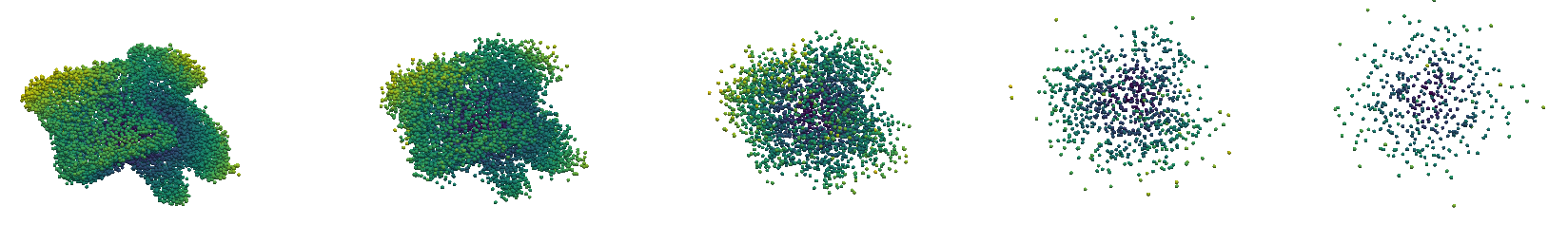
(a)

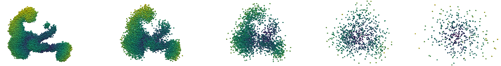
(b)

Figure 5: Additional Qualitative Results on MedShapeNet Dataset. We display reconstructed 3D shapes Spine L3 vertebra and Colon in MedShapeNet dataset which comprise $2.0e^{+3}$ points.

Example: Sampling of MF-CDMs on MedShapeNet. In the experiments targeting a cardinality of $2.0e^{+3}$ on MedShapeNet, we initiate by simulating denoising particle paths starting from a lower cardinality of $N_{0}=1.25e^{+3}$, proceeding until the first branching steps at $\{50\}\in\mathbb{K}^{\prime}/\mathbb{K}^{\prime}$. In the branching step, we apply a point branching function to the simulated particles, which increases to twice the number of particle profiles, $N_{100\in\mathbb{K}^{\prime}}=2.5e^{+3}$. The following diagram provides an overview of how the branching operation increases cardinality during the denoising process:

$$\underbrace{N_{0}\rightarrow\cdots\rightarrow N_{49\in\mathbb{K}/\mathbb{K}^{\prime}}}_{\textbf{Card}:\leavevmode\nobreak\ 1.25e^{+3}}\xlongrightarrow[\Phi^{*}]{\text{Branching}}\underbrace{N_{50\in\mathbb{K}^{\prime}}\rightarrow\cdots\rightarrow N_{99\in\mathbb{K}/\mathbb{K}^{\prime}}}_{\textbf{Card}:\leavevmode\nobreak\ 2.5e^{+3}}\xlongrightarrow[\Phi^{*}]{\text{Branching}}\underbrace{N_{100\in\mathbb{K}^{\prime}}\rightarrow\cdots\rightarrow N_{149}}_{\textbf{Card}:\leavevmode\nobreak\ 5.0e^{+3}}\\ \xlongrightarrow[\Phi^{*}]{\text{Branching}}\underbrace{N_{150\in\mathbb{K}^{\prime}}\rightarrow\cdots\rightarrow N_{199\in\mathbb{K}/\mathbb{K}^{\prime}}}_{\textbf{Card}:1.0e^{+4}}\xlongrightarrow[\Phi^{*}]{\text{Branching}}\underbrace{N_{200\in\mathbb{K}^{\prime}}\rightarrow\cdots\rightarrow N_{299\in\mathbb{K}/\mathbb{K}^{\prime}}}_{\textbf{Card}:2.0e^{+4}}.$$ (172)

Sec A.9.2 provides a detailed algorithmic procedure.

Datasets. This paper utilizes ShapeNet, a widely recognized dataset comprising a vast collection of 3D object models across multiple categories, and MedShapeNet, a curated collection of medical shape data designed for advanced imaging analysis.

1. ShapeNet. (Chang et al., 2015) We adhered to the standard protocol suggested by (Yang et al., 2019) for preprocessing (e.g., random shuffling, normalization) point-sets from 3D shapes, but adjusted the number of points to $10,000$, which is approximately five times larger than the standard setup. All categories were utilized in our experiments.

2. MedShapeNet. (Li et al., 2023) This dataset contains nearly $100,000$ medical shapes, including bones, organs, vessels, muscles, etc., as well as surgical instruments. Our data preprocessing pipeline involves randomizing the arrangement of nodes and selecting a subset of $20,000$ points to form a standardized 3D point cloud. Considering the segmentation of each organ shape into smaller and incomplete parts in the dataset, we focused on utilizing only $1,000$ fully aggregated instances within the dataset. We applied uniform normalization and resized each shape to align within a predefined cubic space of $[-1,1]^{3}\subset\mathbb{R}^{3}$, facilitating comparative and computational analyses.

Neural Network Architectures. In the experiment on a synthetic dataset, we utilized the similar architecture suggested in DPM (Luo & Hu, 2021) for both functions $\mathrm{A}_{\theta}$ and $\mathrm{B}_{\theta}$. In modeling mean-field interaction, we incorporated a local particle association module, akin to the one used in DCGNN (Wang et al., 2019b). This module dynamically pools particles with close geometric proximity during the inference. All experiments were conducted using a setup of $4$ NVIDIA A100 GPUs.

A.9.1 Training Mean-field Chaotic Diffusion Models

This section aims to present the algorithmic implementation of mean-field score matching and training procedure with objective $\mathbf{(P3)}$. We train our score networks based on a mean-field score objective, incorporating the Sobolev norm and reducible network structures. The training procedure is comprehensively outlined in the following three steps.

1. Initialization. Consider an index set $\mathbb{K}=\{0,\cdots,K\}$ for the discrete simulation of SDEs, and its subset $\mathbb{K^{\prime}}\subseteq\mathbb{K}$ for particle branching steps. This operation is selectively applied to steps $k\in\mathbb{K}^{\prime}$ out of the entire sequence of diffusion steps, $\mathbb{K}$. For simplicity, let us denote $\zeta_{t}\coloneqq\mathcal{N}(\mathbf{m}_{\zeta}(t),\sigma_{\zeta}^{2}(t)\mathbf{I}_{d})$, where Gaussian parameters are selected from Appendix C (Song et al., 2021a). Then, we sample $B$ i.i.d particles having a form of

   $$\nu_{t_{k}}\sim\mathbf{Y}_{t_{k}}^{b}=\begin{cases}\mathbf{Y}_{t_{k}}^{b,N_{k}}\sim\zeta_{t_{k}}^{\otimes N_{k}},\quad\forall k\in\mathbb{K}^{\prime},\\ \mathbf{Y}_{t_{k}}^{b,N_{k+1}}\sim(\mathbf{Id}^{\otimes\mathfrak{b}-1}\otimes\Psi^{\theta})_{\#}[\zeta_{t_{k}}^{\otimes N_{k}}],\quad\forall k\in\mathbb{K}\setminus\mathbb{K}^{\prime}.\end{cases}$$ (173)

   Consequently, the cardinality of particles changes with each diffusion step $k$. Specifically, if $k$ belongs to the set for particle branching, $\mathbf{Card}(\nu_{t_{k}})=N_{k+1}$; Otherwise, it remains at $\mathbf{Card}(\nu_{t_{k}})=N_{k}$.

2. Estimation of Sobolev Norm. We first define the discretization of progressively measurable process $\mathcal{G}_{t}^{\theta}$ with respect to $\mathbf{Y}_{t_{k}}^{b}$ and its Jacobian as follows:

   $$\mathcal{G}_{t_{k}}^{\theta}=\mathbf{s}_{\theta}^{\otimes\mathbf{Card}(\nu_{t_{k}})}(t_{k},\mathbf{Y}_{t_{k}}^{b},\nu_{t_{k}})-\nabla\log\zeta_{T-t_{k}}^{\otimes\mathbf{Card}(\nu_{t_{k}})}(\mathbf{Y}_{t_{k}}^{b})$$ (174)

   $$\mathcal{J}\mathcal{G}_{t_{k}}^{\theta}=\mathcal{J}\mathbf{s}_{\theta}^{\otimes\mathbf{Card}(\nu_{t_{k}})}(t_{k},\mathbf{Y}_{t_{k}}^{b},\nu_{t_{k}})-\nabla^{2}\log\zeta_{T-t_{k}}^{\otimes\mathbf{Card}(\nu_{t_{k}})}(\mathbf{Y}_{t_{k}}^{b}),$$ (175)

   where each term $\mathrm{A}_{\theta}^{\otimes N_{k}}$ and $\mathrm{B}_{\theta}$ for score networks $\mathbf{s}_{\theta}^{N_{k}}$ is estimated by the Table A.9.2, Step II. Note that $\mathbf{Card}(\nu_{t_{k}})$ denotes the cardinality of sampled particles.

3. Update Network Parameters. For the calculated estimations above, we update the networks by MF-SM with respect to the subdivision of chaotic entropy, $\mathbf{(P3)}$ in Eq. 28:

   $$\theta\leavevmode\nobreak\ \longleftarrow\leavevmode\nobreak\ \theta-\nabla_{\theta}\frac{1}{B|\mathbb{K}|}\sum_{b}^{B}\sum_{k\in\mathbb{K}}\left[\frac{1}{\mathfrak{b}^{k}}\mathbb{E}\left[{\norm{\mathcal{G}_{t_{k}}^{\theta}}_{E}^{2}+\norm{\mathcal{J}\mathcal{G}_{t_{k}}^{\theta}}_{F}^{2}}\right]\right].$$ (176)

A.9.2 Sampling Scheme for Mean-field Chaos Diffusion Models

To sample the denoising dynamics, this work proposes a modified Euler scheme, adapted for mean-field interacting particle systems (Bossy & Talay, 1997; dos Reis et al., 2022), and approximate the stochastic differential equations in the mean-field limit. The proposed scheme involves a four-step sampling procedure.

1. Initialization. Consider an index set $\mathbb{K}=\{0,\cdots,K\}$ for the discrete simulation of SDEs, and its subset $\mathbb{K^{\prime}}\subseteq\mathbb{K}$ for particle branching steps. In the initial step $k=0$, the probability measure $\varrho_{t_{0}}^{N_{0}}d\mathbf{x}^{N_{k}}$ is set to $N_{0}$-product of standard Gaussian density, $\textit{i}.\textit{e}.,\mathcal{N}^{\otimes N_{0}}(\mathbf{I}_{N_{0}d})$. For the steps $k>0$, we sample i.i.d $B$ particles from the branched probability measure obtained in the previous step: $\{\mathbf{X}_{t_{k}}^{b,N_{k}}\}_{b\leq B}\sim\varrho_{t_{k}}^{N_{k}}d\mathbf{x}^{N_{k}}.$

2. Estimation of Vector fields. Given sampled $(N_{k}d)$-dimensional $B$ vectors in the previous step, we estimate the vector fields in this step. Recall that the vector fields are given as $\nabla V^{N}(t,\mathbf{x},\nu_{t}^{N};\theta)\coloneqq f_{t}^{\otimes N}(\mathbf{x})-\sigma_{t}^{2}\mathbf{s}_{\theta}(t,\mathbf{x},\nu_{t})$. Given the definition of MF VP-SDE where $(\beta_{\text{max}},\beta_{\text{min}})=(20,0.1)$, we have

   $$f_{t}^{\otimes N_{k}}(\mathbf{X}_{t}^{b,N_{k}})=-\frac{\beta_{t}}{2}\mathbf{X}_{t}^{b,N_{k}},\quad\beta_{t}=\beta_{\text{min}}+t(\beta_{\text{max}}-\beta_{\text{min}}),\quad b\leq B.$$ (177)

   To estimate $\mathrm{A}_{\theta}$, we adhere to the definition of a reducible architecture explored in Sec A.3, namely, the concatenation of equi-weighted, identical networks.

   $$\mathrm{A}_{\theta}^{\otimes N_{k}}(t_{k},\mathbf{X}_{t_{k}}^{b,N_{k}})=\frac{1}{N_{k}}[\mathrm{A}_{\theta}(t_{k},\mathbf{X}_{t_{k}}^{b,1,N_{k}}),\cdots,\mathrm{A}_{\theta}(t_{k},\mathbf{X}_{t_{k}}^{b,N_{k},N_{k}})]^{T}\in\mathcal{X}^{N_{k}}.$$ (178)

   The mean-field interaction is formally redefined in the following manner: it involves the projection of the probability measure as $\pi_{\#}^{i}\nu_{t}^{N_{k}}=\nu_{t}^{i,N_{k}}\sim\{\mathbf{X}_{t_{k}}^{b,i,N_{k}}\}_{b\leq B}$:

   $$\quad\left([\mathrm{B}_{\theta}*\nu_{\mathbb{B}_{R}}^{i}](\mathbf{X}_{t_{k}}^{b,N_{k}})\right)^{\otimes N_{k}}=\frac{1}{N_{k}}\left[[\mathrm{B}*\pi^{1}_{\#}\nu_{t_{k}}^{N_{k}}],\cdots,[\mathrm{B}*{\pi_{\#}}_{t_{k}}^{N_{k}}]\right]^{T}(\mathbf{X}_{t_{k}}^{b,N_{k}}).$$ (179)

   With the finite cut-off radius $R$, we consider Euclidean balls to define truncated convolution:

   $$\mathbb{B}_{R}\coloneqq\mathbb{B}_{R}^{\mathbf{x}=\mathbf{X}_{t_{k}}^{b,i,N_{k}}}=\left\{\mathbf{y};d_{E}^{2}(\mathbf{y},\mathbf{X}_{t_{k}}^{b,i,N_{k}})\leq R\right\}.$$ (180)

   Given definition above, each component in Eq. 179 is given by

   $$\begin{split}[\mathrm{B}_{\theta}*\nu_{\mathbb{B}_{R}}^{i}](\mathbf{X}_{t_{k}}^{b,i,N_{k}})&\propto\frac{1}{N_{k}-1}\sum_{i\neq j}^{N_{k}}\int_{\mathbb{B}_{R}}\mathrm{B}_{\theta}(\mathbf{X}_{t_{k}}^{b,i,N_{k}}-\mathbf{X}_{t_{k}}^{b,j,N_{k}})\nu_{t_{k}}^{j,N_{k}}(d\mathbf{X}_{t_{k}}^{b,i,N_{k}}).\end{split}$$ (181)

3. Applying Euler Schemes. Having collected estimated terms from the previous step, we apply the Euler scheme to have particle simulation of dWGFs accordingly.

   $$\mathbf{X}_{t_{k+1}}^{b,N_{k}}=\mathbf{X}_{t_{k}}^{b,N_{k}}+\nabla V^{N}(t,\mathbf{X}_{t_{k}}^{b,N_{k}},\nu_{t_{k}}^{N_{k}};\theta)\Delta_{t}+\sqrt{\beta_{t}}\Delta_{t}B_{t_{k}}^{N_{k}},\quad b\leq B,$$ (182)

   where $\Delta_{t}B_{t_{k}}^{N_{k}}\coloneqq B_{t_{k}}^{N_{k}}-B_{t_{k-1}}^{N_{k}}\sim\mathcal{N}[\Delta_{t}I_{d{N_{k}}}]$.

4. Particle Branching. In the final step, we apply the particle branching operation to enhance the cardinality. This operation is selectively applied to steps $k\in\mathbb{K}^{\prime}$ out of the entire sequence of diffusion steps, $\mathbb{K}$.

   $$[\mathbf{X}_{t_{k}}^{B,\otimes(\mathfrak{b}-1)N_{k}},\leavevmode\nobreak\ \Psi_{\theta}(\mathbf{X}_{t_{k}}^{B,N_{k}})]\leavevmode\nobreak\ \rightharpoonup\leavevmode\nobreak\ \mathbf{X}_{t_{k}}^{B,N_{k+1}},\quad(\mathbf{Id}^{\otimes\mathfrak{b}-1}\otimes\Psi^{\theta}_{N_{k+1}})_{\#}[\varrho_{t_{k}}^{N_{k}}]\leavevmode\nobreak\ \rightharpoonup\leavevmode\nobreak\ \varrho_{t_{k}}^{N_{k+1}}d\mathbf{x}^{N_{k+1}}.$$ (183)

   When branching particles, the cardinality grows as $N_{k+1}=\mathfrak{b}N_{k}$, and the entire sampling scheme is repeated until reaching the final step $k\rightarrow K$.

References

• Adams & Fournier (2003) Adams, R. A. and Fournier, J. J. Sobolev spaces. Elsevier, 2003.
• Anonymous (2023) Anonymous. Score-based generative models break the curse of dimensionality in learning a family of sub-gaussian distributions. In Submitted to The Twelfth International Conference on Learning Representations, 2023. under review.
• Anstine & Isayev (2023) Anstine, D. M. and Isayev, O. Generative models as an emerging paradigm in the chemical sciences. Journal of the American Chemical Society, 145(16):8736–8750, 2023.
• Bakry (1997) Bakry, D. On sobolev and logarithmic sobolev inequalities for markov semigroups. New trends in stochastic analysis (Charingworth, 1994), pp. 43–75, 1997.
• Bakry et al. (2014) Bakry, D., Gentil, I., Ledoux, M., et al. Analysis and geometry of Markov diffusion operators, volume 103. Springer, 2014.
• Beaulieu-Jones et al. (2019) Beaulieu-Jones, B. K., Wu, Z. S., Williams, C., Lee, R., Bhavnani, S. P., Byrd, J. B., and Greene, C. S. Privacy-preserving generative deep neural networks support clinical data sharing. Circulation: Cardiovascular Quality and Outcomes, 12(7):e005122, 2019.
• Bensoussan et al. (2013) Bensoussan, A., Frehse, J., Yam, P., et al. Mean field games and mean field type control theory, volume 101. Springer, 2013.
• Bensoussan et al. (2017) Bensoussan, A., Frehse, J., and Yam, S. C. P. On the interpretation of the master equation. Stochastic Processes and their Applications, 127(7):2093–2137, 2017.
• Bolley (2010) Bolley, F. Quantitative concentration inequalities on sample path space for mean field interaction. ESAIM: Probability and Statistics, 14:192–209, 2010. doi: 10.1051/ps:2008033.
• Bolley et al. (2007) Bolley, F., Guillin, A., and Villani, C. Quantitative concentration inequalities for empirical measures on non-compact spaces. Probability Theory and Related Fields, 137:541–593, 2007.
• Bossy & Talay (1997) Bossy, M. and Talay, D. A stochastic particle method for the mckean-vlasov and the burgers equation. Mathematics of computation, 66(217):157–192, 1997.
• Brezis & Brézis (2011) Brezis, H. and Brézis, H. Functional analysis, Sobolev spaces and partial differential equations, volume 2. Springer, 2011.
• Cardaliaguet (2010) Cardaliaguet, P. Notes on mean field games. Technical report, Technical report, 2010.
• Cardaliaguet & Lehalle (2018) Cardaliaguet, P. and Lehalle, C.-A. Mean field game of controls and an application to trade crowding. Mathematics and Financial Economics, 12:335–363, 2018.
• Carmona & Delarue (2013) Carmona, R. and Delarue, F. Probabilistic analysis of mean-field games. SIAM Journal on Control and Optimization, 51(4):2705–2734, 2013.
• Carmona & Delarue (2015) Carmona, R. and Delarue, F. Forward–backward stochastic differential equations and controlled mckean–vlasov dynamics. 2015.
• Carmona & Laurière (2021) Carmona, R. and Laurière, M. Convergence analysis of machine learning algorithms for the numerical solution of mean field control and games i: the ergodic case. SIAM Journal on Numerical Analysis, 59(3):1455–1485, 2021.
• Carmona & Laurière (2022) Carmona, R. and Laurière, M. Convergence analysis of machine learning algorithms for the numerical solution of mean field control and games: Ii—the finite horizon case. The Annals of Applied Probability, 32(6):4065–4105, 2022.
• Carmona et al. (2018) Carmona, R., Delarue, F., et al. Probabilistic theory of mean field games with applications I-II. Springer, 2018.
• Carrillo et al. (2003) Carrillo, J. A., McCann, R. J., and Villani, C. Kinetic equilibration rates for granular media and related equations: entropy dissipation and mass transportation estimates. Revista Matematica Iberoamericana, 19(3):971–1018, 2003.
• Carrillo et al. (2006) Carrillo, J. A., McCann, R. J., and Villani, C. Contractions in the 2-wasserstein length space and thermalization of granular media. Archive for Rational Mechanics and Analysis, 179:217–263, 2006.
• Chaintron & Diez (2022) Chaintron, L.-P. and Diez, A. Propagation of chaos: A review of models, methods and applications. .. applications. Kinetic and Related Models, 15(6):1017–1173, 2022.
• Chang et al. (2015) Chang, A. X., Funkhouser, T., Guibas, L., Hanrahan, P., Huang, Q., Li, Z., Savarese, S., Savva, M., Song, S., Su, H., et al. Shapenet: An information-rich 3d model repository. arXiv preprint arXiv:1512.03012, 2015.
• Chen et al. (2023) Chen, H., Lee, H., and Lu, J. Improved analysis of score-based generative modeling: User-friendly bounds under minimal smoothness assumptions. In International Conference on Machine Learning, pp. 4735–4763. PMLR, 2023.
• Chen et al. (2021) Chen, T., Liu, G.-H., and Theodorou, E. A. Likelihood training of schr$\backslash$” odinger bridge using forward-backward sdes theory. arXiv preprint arXiv:2110.11291, 2021.
• Collet & Malrieu (2008) Collet, J.-F. and Malrieu, F. Logarithmic sobolev inequalities for inhomogeneous markov semigroups. ESAIM: Probability and Statistics, 12:492–504, 2008.
• Daskalakis et al. (2009) Daskalakis, C., Goldberg, P. W., and Papadimitriou, C. H. The complexity of computing a nash equilibrium. SIAM Journal on Computing, 39(1):195–259, 2009.
• De Bortoli (2022) De Bortoli, V. Convergence of denoising diffusion models under the manifold hypothesis. arXiv preprint arXiv:2208.05314, 2022.
• Del Moral (2013) Del Moral, P. Mean field simulation for Monte Carlo integration. CRC press, 2013.
• Dembo & Zeitouni (2009) Dembo, A. and Zeitouni, O. Large deviations techniques and applications, volume 38. Springer Science & Business Media, 2009.
• Dockhorn et al. (2022) Dockhorn, T., Vahdat, A., and Kreis, K. Score-based generative modeling with critically-damped langevin diffusion. In International Conference on Learning Representations, 2022.
• Dos Reis & Platonov (2023) Dos Reis, G. and Platonov, V. Itô-wentzell-lions formula for measure dependent random fields under full and conditional measure flows. Potential Analysis, 59(3):1313–1344, 2023.
• dos Reis et al. (2022) dos Reis, G., Engelhardt, S., and Smith, G. Simulation of mckean–vlasov sdes with super-linear growth. IMA Journal of Numerical Analysis, 42(1):874–922, 2022.
• Dutordoir et al. (2023) Dutordoir, V., Saul, A., Ghahramani, Z., and Simpson, F. Neural diffusion processes, 2023.
• Ethier & Kurtz (2009) Ethier, S. N. and Kurtz, T. G. Markov processes: characterization and convergence. John Wiley & Sons, 2009.
• Fournier & Guillin (2015) Fournier, N. and Guillin, A. On the rate of convergence in wasserstein distance of the empirical measure. Probability theory and related fields, 162(3-4):707–738, 2015.
• Franceschi et al. (2023) Franceschi, J.-Y., Gartrell, M., Santos, L. D., Issenhuth, T., de Bézenac, E., Chen, M., and Rakotomamonjy, A. Unifying gans and score-based diffusion as generative particle models, 2023.
• Germain et al. (2022) Germain, M., Mikael, J., and Warin, X. Numerical resolution of mckean-vlasov fbsdes using neural networks. Methodology and Computing in Applied Probability, 24(4):2557–2586, 2022.
• Gottlieb (1998) Gottlieb, A. D. Markov transitions and the propagation of chaos. University of California, Berkeley, 1998.
• Guillin et al. (2021) Guillin, A., Liu, W., Wu, L., and Zhang, C. The kinetic fokker-planck equation with mean field interaction. Journal de Mathématiques Pures et Appliquées, 150:1–23, 2021.
• Guo et al. (2023) Guo, X., Pham, H., and Wei, X. Itô’s formula for flows of measures on semimartingales. Stochastic Processes and their Applications, 159:350–390, 2023.
• Hagemann et al. (2023) Hagemann, P., Ruthotto, L., Steidl, G., and Yang, N. T. Multilevel diffusion: Infinite dimensional score-based diffusion models for image generation. arXiv preprint arXiv:2303.04772, 2023.
• Han et al. (2022) Han, J., Hu, R., and Long, J. Learning high-dimensional mckean-vlasov forward-backward stochastic differential equations with general distribution dependence. arXiv preprint arXiv:2204.11924, 2022.
• Hauray & Mischler (2014) Hauray, M. and Mischler, S. On kac’s chaos and related problems. Journal of Functional Analysis, 266(10):6055–6157, 2014.
• Ho & Salimans (2022) Ho, J. and Salimans, T. Classifier-free diffusion guidance, 2022.
• Hoogeboom et al. (2022) Hoogeboom, E., Satorras, V. G., Vignac, C., and Welling, M. Equivariant diffusion for molecule generation in 3d. In International conference on machine learning, pp. 8867–8887. PMLR, 2022.
• Jabin & Wang (2017) Jabin, P.-E. and Wang, Z. Mean field limit for stochastic particle systems. Active Particles, Volume 1: Advances in Theory, Models, and Applications, pp.  379–402, 2017.
• Jo et al. (2022) Jo, J., Lee, S., and Hwang, S. J. Score-based generative modeling of graphs via the system of stochastic differential equations. In International Conference on Machine Learning, pp. 10362–10383. PMLR, 2022.
• Kac (1956) Kac, M. Foundations of kinetic theory. In Proceedings of The third Berkeley symposium on mathematical statistics and probability, volume 3, pp.  171–197, 1956.
• Kadanoff (2009) Kadanoff, L. P. More is the same; phase transitions and mean field theories. Journal of Statistical Physics, 137:777–797, 2009.
• Kaissis et al. (2020) Kaissis, G. A., Makowski, M. R., Rückert, D., and Braren, R. F. Secure, privacy-preserving and federated machine learning in medical imaging. Nature Machine Intelligence, 2(6):305–311, 2020.
• Karniadakis et al. (2021) Karniadakis, G. E., Kevrekidis, I. G., Lu, L., Perdikaris, P., Wang, S., and Yang, L. Physics-informed machine learning. Nature Reviews Physics, 3(6):422–440, 2021.
• Karras et al. (2017) Karras, T., Aila, T., Laine, S., and Lehtinen, J. Progressive growing of gans for improved quality, stability, and variation. arXiv preprint arXiv:1710.10196, 2017.
• Kerrigan et al. (2023) Kerrigan, G., Ley, J., and Smyth, P. Diffusion generative models in infinite dimensions. In International Conference on Artificial Intelligence and Statistics, pp.  9538–9563. PMLR, 2023.
• Kim et al. (2021) Kim, J., Yoo, J., Lee, J., and Hong, S. Setvae: Learning hierarchical composition for generative modeling of set-structured data. In Proceedings of the IEEE/CVF Conference on Computer Vision and Pattern Recognition, pp.  15059–15068, 2021.
• Kloeckner (2010) Kloeckner, B. A geometric study of wasserstein spaces: Euclidean spaces. Annali della Scuola Normale Superiore di Pisa-Classe di Scienze, 9(2):297–323, 2010.
• Koehl & Delarue (1994) Koehl, P. and Delarue, M. Application of a self-consistent mean field theory to predict protein side-chains conformation and estimate their conformational entropy. Journal of molecular biology, 239(2):249–275, 1994.
• Kolouri et al. (2019) Kolouri, S., Nadjahi, K., Simsekli, U., Badeau, R., and Rohde, G. Generalized sliced wasserstein distances. Advances in neural information processing systems, 32, 2019.
• Koshizuka & Sato (2023) Koshizuka, T. and Sato, I. Neural lagrangian schr\”{o}dinger bridge: Diffusion modeling for population dynamics. In The Eleventh International Conference on Learning Representations, 2023.
• Kunita (1997) Kunita, H. Stochastic flows and stochastic differential equations, volume 24. Cambridge university press, 1997.
• Lachapelle et al. (2010) Lachapelle, A., Salomon, J., and Turinici, G. Computation of mean field equilibria in economics. Mathematical Models and Methods in Applied Sciences, 20(04):567–588, 2010.
• Ledoux (2006) Ledoux, M. Concentration of measure and logarithmic sobolev inequalities. In Seminaire de probabilites XXXIII, pp.  120–216. Springer, 2006.
• Lee et al. (2022) Lee, H., Lu, J., and Tan, Y. Convergence for score-based generative modeling with polynomial complexity. In Oh, A. H., Agarwal, A., Belgrave, D., and Cho, K. (eds.), Advances in Neural Information Processing Systems, 2022.
• Li et al. (2023) Li, J., Pepe, A., Gsaxner, C., Luijten, G., Jin, Y., Ambigapathy, N., Nasca, E., Solak, N., Melito, G. M., Memon, A. R., et al. Medshapenet–a large-scale dataset of 3d medical shapes for computer vision. arXiv preprint arXiv:2308.16139, 2023.
• Lim et al. (2023) Lim, S., Yoon, E., Byun, T., Kang, T., Kim, S., Lee, K., and Choi, S. Score-based generative modeling through stochastic evolution equations in hilbert spaces. In Thirty-seventh Conference on Neural Information Processing Systems, 2023.
• Liu et al. (2022) Liu, G.-H., Chen, T., So, O., and Theodorou, E. Deep generalized schrödinger bridge. In Advances in Neural Information Processing Systems, 2022.
• Lott (2008) Lott, J. Some geometric calculations on wasserstein space. Communications in Mathematical Physics, 277(2):423–437, 2008.
• Lu et al. (2022) Lu, C., Zheng, K., Bao, F., Chen, J., Li, C., and Zhu, J. Maximum likelihood training for score-based diffusion odes by high order denoising score matching. In International Conference on Machine Learning, pp. 14429–14460. PMLR, 2022.
• Lu et al. (2023) Lu, J., Wu, Y., and Xiang, Y. Score-based transport modeling for mean-field fokker-planck equations. arXiv preprint arXiv:2305.03729, 2023.
• Luo & Hu (2021) Luo, S. and Hu, W. Diffusion probabilistic models for 3d point cloud generation. In Proceedings of the IEEE/CVF Conference on Computer Vision and Pattern Recognition, pp.  2837–2845, 2021.
• Malagò et al. (2018) Malagò, L., Montrucchio, L., and Pistone, G. Wasserstein riemannian geometry of gaussian densities. Information Geometry, 1:137–179, 2018.
• Malrieu (2001) Malrieu, F. Logarithmic sobolev inequalities for some nonlinear pde’s. Stochastic processes and their applications, 95(1):109–132, 2001.
• Malrieu (2003) Malrieu, F. Convergence to equilibrium for granular media equations and their euler schemes. The Annals of Applied Probability, 13(2):540–560, 2003.
• Niu et al. (2020) Niu, C., Song, Y., Song, J., Zhao, S., Grover, A., and Ermon, S. Permutation invariant graph generation via score-based generative modeling. In International Conference on Artificial Intelligence and Statistics, pp.  4474–4484. PMLR, 2020.
• Øksendal & Øksendal (2003) Øksendal, B. and Øksendal, B. Stochastic differential equations. Springer, 2003.
• Otto & Villani (2000) Otto, F. and Villani, C. Generalization of an inequality by talagrand and links with the logarithmic sobolev inequality. Journal of Functional Analysis, 173(2):361–400, 2000.
• Panaretos & Zemel (2019) Panaretos, V. M. and Zemel, Y. Statistical aspects of wasserstein distances. Annual review of statistics and its application, 6:405–431, 2019.
• Park et al. (2023) Park, S., Park, B., Lee, M., and Lee, C. Neural stochastic differential games for time-series analysis. In Proceedings of the 40th International Conference on Machine Learning, ICML’23, 2023.
• Pidstrigach et al. (2023) Pidstrigach, J., Marzouk, Y., Reich, S., and Wang, S. Infinite-dimensional diffusion models for function spaces. arXiv preprint arXiv:2302.10130, 2023.
• Qi et al. (2017a) Qi, C. R., Yi, L., Su, H., and Guibas, L. J. Pointnet++: Deep hierarchical feature learning on point sets in a metric space. Advances in neural information processing systems, 30, 2017a.
• Qi et al. (2017b) Qi, C. R., Yi, L., Su, H., and Guibas, L. J. Pointnet++: Deep hierarchical feature learning on point sets in a metric space. Advances in neural information processing systems, 30, 2017b.
• Rasul et al. (2021) Rasul, K., Seward, C., Schuster, I., and Vollgraf, R. Autoregressive denoising diffusion models for multivariate probabilistic time series forecasting. In International Conference on Machine Learning, pp. 8857–8868. PMLR, 2021.
• Rezende & Mohamed (2015) Rezende, D. and Mohamed, S. Variational inference with normalizing flows. In International conference on machine learning, pp. 1530–1538. PMLR, 2015.
• Rombach et al. (2022) Rombach, R., Blattmann, A., Lorenz, D., Esser, P., and Ommer, B. High-resolution image synthesis with latent diffusion models. In Proceedings of the IEEE/CVF Conference on Computer Vision and Pattern Recognition, pp.  10684–10695, 2022.
• Ruthotto et al. (2020) Ruthotto, L., Osher, S. J., Li, W., Nurbekyan, L., and Fung, S. W. A machine learning framework for solving high-dimensional mean field game and mean field control problems. Proceedings of the National Academy of Sciences, 117(17):9183–9193, 2020.
• Santambrogio (2015) Santambrogio, F. Optimal transport for applied mathematicians. Birkäuser, NY, 55(58-63):94, 2015.
• Santambrogio (2017) Santambrogio, F. $\{$Euclidean, metric, and Wasserstein$\}$ gradient flows: an overview. Bulletin of Mathematical Sciences, 7:87–154, 2017.
• Shi et al. (2023) Shi, Y., Bortoli, V. D., Campbell, A., and Doucet, A. Diffusion schrödinger bridge matching. In Thirty-seventh Conference on Neural Information Processing Systems, 2023.
• Song et al. (2021a) Song, J., Meng, C., and Ermon, S. Denoising diffusion implicit models. In International Conference on Learning Representations, 2021a.
• Song et al. (2021b) Song, Y., Durkan, C., Murray, I., and Ermon, S. Maximum likelihood training of score-based diffusion models. Advances in Neural Information Processing Systems, 34:1415–1428, 2021b.
• Song et al. (2021c) Song, Y., Sohl-Dickstein, J., Kingma, D. P., Kumar, A., Ermon, S., and Poole, B. Score-based generative modeling through stochastic differential equations. In International Conference on Learning Representations, 2021c.
• Song et al. (2023) Song, Y., Dhariwal, P., Chen, M., and Sutskever, I. Consistency models, 2023.
• Strocchi et al. (2020) Strocchi, M., Augustin, C. M., Gsell, M. A., Karabelas, E., Neic, A., Gillette, K., Razeghi, O., Prassl, A. J., Vigmond, E. J., Behar, J. M., et al. A publicly available virtual cohort of four-chamber heart meshes for cardiac electro-mechanics simulations. PloS one, 15(6):e0235145, 2020.
• Sznitman (1991a) Sznitman, A.-S. Topics in propagation of chaos. Lecture notes in mathematics, pp.  165–251, 1991a.
• Sznitman (1991b) Sznitman, A.-S. Topics in propagation of chaos. In Ecole d’Eté de Probabilités de Saint-Flour XIX — 1989, pp.  165–251. Springer Berlin Heidelberg, 1991b.
• Tashiro et al. (2021) Tashiro, Y., Song, J., Song, Y., and Ermon, S. Csdi: Conditional score-based diffusion models for probabilistic time series imputation. Advances in Neural Information Processing Systems, 34:24804–24816, 2021.
• Thorpe et al. (2022) Thorpe, M., Nguyen, T. M., Xia, H., Strohmer, T., Bertozzi, A., Osher, S., and Wang, B. GRAND++: Graph neural diffusion with a source term. In International Conference on Learning Representations, 2022.
• Tyszkiewicz et al. (2023) Tyszkiewicz, M. J., Fua, P., and Trulls, E. Gecco: Geometrically-conditioned point diffusion models. arXiv preprint arXiv:2303.05916, 2023.
• Villani (2006) Villani, C. Hypocoercivity, 2006.
• Wang et al. (2019a) Wang, Y., Sun, Y., Liu, Z., Sarma, S. E., Bronstein, M. M., and Solomon, J. M. Dynamic graph cnn for learning on point clouds. ACM Transactions on Graphics (tog), 38(5):1–12, 2019a.
• Wang et al. (2019b) Wang, Y. et al. Dynamic graph cnn for learning on point clouds. ACM Transactions on Graphics, 38(5):146, 2019b.
• Xu et al. (2023) Xu, M., Powers, A. S., Dror, R. O., Ermon, S., and Leskovec, J. Geometric latent diffusion models for 3d molecule generation. In International Conference on Machine Learning, pp. 38592–38610. PMLR, 2023.
• Yang et al. (2019) Yang, G., Huang, X., Hao, Z., Liu, M.-Y., Belongie, S., and Hariharan, B. Pointflow: 3d point cloud generation with continuous normalizing flows. In Proceedings of the IEEE/CVF international conference on computer vision, pp.  4541–4550, 2019.
• Zaheer et al. (2017) Zaheer, M., Kottur, S., Ravanbakhsh, S., Poczos, B., Salakhutdinov, R. R., and Smola, A. J. Deep sets. Advances in neural information processing systems, 30, 2017.
• Zeng et al. (2022) Zeng, X., Vahdat, A., Williams, F., Gojcic, Z., Litany, O., Fidler, S., and Kreis, K. Lion: Latent point diffusion models for 3d shape generation. In Advances in Neural Information Processing Systems, 2022.
• Zhao et al. (2016) Zhao, J., Mathieu, M., and LeCun, Y. Energy-based generative adversarial networks. In International Conference on Learning Representations, 2016.
• Zhou et al. (2021) Zhou, L., Du, Y., and Wu, J. 3d shape generation and completion through point-voxel diffusion. In Proceedings of the IEEE/CVF International Conference on Computer Vision, pp.  5826–5835, 2021.