Exploiting Monotonicity to Design an Adaptive PI Passivity-Based Controller for a Fuel-Cell System

Abstract

We present a controller for a power electronic system composed of a fuel cell (FC) connected to a boost converter which feeds a resistive load. The controller aims to regulate the output voltage of the converter regardless of the uncertainty of the load. Leveraging the monotonicity feature of the fuel cell polarization curve we prove that the nonlinear system can be controlled by means of a passivity-based proportional-integral controller. We afterward extend the result to an adaptive version, allowing the controller to deal with parameter uncertainties, such as inductor parasitic resistance, load, and FC polarization curve parameters. This adaptive design is based on an indirect control approach with online parameter identification performed by a “hybrid” estimator which combines two techniques: the gradient-descent and immersion-and-invariance algorithms. The overall system is proved to be stable with the output voltage regulated to its reference. Experimental results validate our proposal under two real-life scenarios: pulsating load and output voltage reference changes.

I Introduction

A clean and non-intermittent source that is helping in the goal of CO2 reduction is the hydrogen fuel cell (FC) [1]. This device efficiently converts chemical energy into electrical energy using an electrochemical reaction that consumes oxygen and hydrogen to generate electrical energy, water, and heat. Much study in recent years has focused on the Proton-Exchange Membrane FC (PEMFC), a type of FC that stands out for its high power density, rapid start-up, versatility, and low operating temperature, among others [2]. Possible applications of PEMFCs are transportation electrification and microgrids [3]. In addition, due to the non-linear relationship between the output current and voltage, it is required to employ a power converter as an interface between the PEMFC and a DC link, forming a FC system. This converter routes energy from the FC to the load at voltage levels compatible with the operation of the load. However, advanced control algorithms are necessary to drive the overall operation of this FC system, to ensure tight output voltage regulation despite load changes, to meet specific dynamic responses, and to have robustness against parameter uncertainties. Furthermore, each PEMFC exhibits a characteristic current and voltage relationship in a steady-state operation called polarization curve, which is a widely used diagnostic approach for evaluating the performance of a PEMFC [4]. This plot can be mathematically characterized using empirical models that include nonlinear functions of the current and constant parameters to approximate the voltage drops experienced in a real PEMFC. For instance, a nonlinear static model, which uses three parameters is detailed in [5]. Another case is the fifth-order polynomial model given in [6]. Moreover, in [7], the well-known Larminie-Dicks model is detailed, where the voltage losses (activation, ohmic, and concentration) are taken into account. Additionally, in [8], a two-termed power function model is detailed, where the parameters are the open circuit voltage and two positive constants. In general, to accurately predict the operation of the FC, the knowledge of model parameters is crucial. A way to determine these values is through offline estimation with data-fitting procedures, performed before the system starts its operation. However, in a real setting, these parameters are sensible to several factors such as temperature, humidity, etc. As a result of that, they change slowly while the system operation is in progress. In this regard, online estimation provides a solution to deal with these variations by continuously updating these estimates while the system operates. For example, in [9], the parameters for a nonlinear PEMFC model are estimated online. To obtain the regressor, its nonlinear parametric model is linearized using Taylor series expansion. Then, an adaptive estimator is designed to achieve exponential parameter convergence, proved via Lyapunov stability theory. Experimental results validate the correct performance of this estimator. On the other hand, in [10] an online parameter estimator of a PEMFC modeled by an equivalent electrical circuit is designed. Its objective is the assessment of a PEMFC remaining useful life. For this, a Lyapunov-based adaptive law is developed. It proves asymptotic stability and parameter convergence and its performance is validated through experimental results.

In this work, we consider a system composed of a PEMFC, a boost converter, and a load. As a control problem, the derivation of control strategies that permit the voltage regulation of the system poses a challenge due to the non-linearities describing the behavior of the FC. Besides, due to the non-minimum phase (NMP) behavior, the output voltage regulation of the boost converter is carried out indirectly, through current mode control (CMC) [11]. As widely reported, this issue is circumvented by a scheme consisting of two control loops, each one evolving in a different time scale: a “voltage” outer loop and a “current” inner loop. The rationale of this control strategy is the following. The inner control loop regulates the current to a desired reference. On the other hand, the outer loop regulates the voltage to its setpoint by providing to the inner loop the corresponding reference of the current that makes possible such task. Traditionally, the voltage loop is implemented with a proportional-integral (PI) controller, and the current loop with linear or non-linear controllers, such as passivity-based control (PBC), backstepping, and sliding mode control, among others. In particular, for the system under consideration, the CMC scheme is employed in [12], where the inner current loop is designed with backstepping control, and the outer voltage loop is designed using a classical PI action over the output voltage. Moreover, in [13], the current loop is designed with classical PBC, and the robustness of this CMC scheme is enhanced by online estimating of the parasitic resistance of the inductor and the load conductance using Immersion and Invariance (I&I) [14]. In these previous works, Lyapunov stability is demonstrated, tight voltage regulation is obtained, and the PEMFC is modeled with a two-termed power function with their parameters estimated with offline data fitting procedures. On the other hand, a simplified scheme using a single control PI loop, based on passivity, is presented in [7], where offline estimation of the PEMFC parameters and online estimation of the load are performed to compute the equilibrium points required by the proposed controller. This approach exploits the monotonic nature of the polarization curve to design the control scheme. Relying on this property, the practical stability of the system operation is proven for the joint operation of the controller with the estimator.

In this work, an improvement of the adaptive controller designed in [7] is presented. This is done by adding the gradient-descent (online) algorithm [15]—a standard approach in engineering applications—to estimate the FC parameters. The algorithm operates simultaneously with an I&I algorithm, which estimates the converter parameters. This enables the online estimation of the equilibrium point required by the PI-PBC scheme. Besides, in this note, it is also proven exponential stability of the controller when all parameters are known and asymptotically stability of the overall adaptive system. Finally, we remark that as far as the authors’ knowledge, there is no previous work in literature where the FC polarization curve is estimated online in closed-loop operation.

The rest of the paper is organized as follows. Section 2 presents the FC system under study and introduces the PI-PBC assuming the parameters are known. Then, in Section 3, this controller is turned adaptive with an online estimator based on I&I and gradient-descent theory. Experimental results revealing the closed-loop performance of the system are presented in Section 4. Finally, in Section 5, the conclusions of the results are presented and suggestions for further research are provided.

Notation. $I_{n}$ corresponds to the $n\times n$ identity matrix. When clear from the context the arguments of the functions are omitted. Given a full-rank matrix $G(x)\in\mathbb{R}^{n\times m}$, with $n>m$, we denote its left annihilator as $G^{\perp}(x)\in\mathbb{R}^{(n-m)\times n}$ and its pseudo inverse as $G^{+}(x):=[G^{\top}(x)G(x)]^{-1}G^{\top}(x)$—i.e., they satisfy $G^{\perp}G=0$ and $G^{+}G=I_{m}$. We denote $v_{i}$ as a vector of the standard basis with its $i$-th element equal to one—its dimension can be inferred from the context. We refer to $\mathcal{L}_{2}$ as the set of square-integrable functions $f:\mathbb{R}_{+}\to\mathbb{R}$, namely, they satisfy $\int_{0}^{\infty}|f(t)|^{2}dt<\infty.$

II System description and control

The electrical circuit of the FC system under consideration is given in Fig. 1. As can be seen from the figure, the system is composed of a PEMFC which feeds a load through a protective diode $D_{p}$ and a boost DC-DC converter. The converter regulates the output voltage to which the load is connected. This voltage is kept constant at a desired setpoint regardless of how much power it is being consumed by the load.

The model of the system in Fig. 1 is represented by the equations [7, 16]

$$C_{fc}\dot{v}_{fc}= i_{fc}-i_{L},$$ (1a)

$$L\dot{i}_{L}= -R_{p}i_{L}+v_{fc}-(1-D)v_{o},$$ (1b)

$$C\dot{v}_{o}= -v_{o}/R_{L}+(1-D)i_{L},$$ (1c)

where $C_{fc}$ and $C$ are the coupling fuel-cell capacitor and output converter capacitor, respectively. Also, $L$ is the converter inductance, $R_{p}$ is the inductor parasitic resistance, $R_{L}$ is the load resistance. The signal $D\in(0,1)$ corresponds to the converter duty cycle. On the other hand, $v_{o}$ is the capacitor output voltage, whereas $v_{fc}$ and $i_{fc}$ are the fuel-cell voltage and current, respectively. These two last variables relate to each other by means of the polarization curve [8]

$$I_{fc}(v_{fc}):=i_{fc}=\left(\frac{E_{oc}-v_{fc}}{\theta_{s1}}\right)^{\frac{1}{\theta_{s2}}},$$ (2)

where $E_{oc}\geq 0$ refers to the open-circuit voltage of the FC. Also, the parameters $\theta_{s1}$ and $\theta_{s2}$ are positive. According with the physical operation of the FC System, its current and voltage variables satisfy the following

• $v_{fc}$ is nonnegative and $E_{oc}-v_{fc}>0.$

• $i_{fc}$ and $v_{o}$ are nonnegative.

Therefore, P1 and P2 are standing assumptions throughout this note.

Fact 1

The relation between the voltage and current in the function $-I_{fc}$ is strongly monotonic. Namely, for any scalars $a$ and $b$ satisfying P1, there exists a constant $\alpha>0$ such that the following inequality holds

$$(a-b)\Big{[}[-I_{fc}(a)]-[-I_{fc}(b)]\Big{]}\geq\alpha(a-b)^{2}.$$ (3)

Proof:

The derivative of $-I_{fc}$ with respect to $v_{fc}$ is

$$\frac{d}{dv_{fc}}[-I_{fc}(v_{fc})]=\frac{1}{\theta_{s1}\theta_{s2}}\left(\frac{E_{oc}-v_{fc}}{\theta_{s1}}\right)^{\frac{1}{\theta_{s2}}-1},$$

which is positive, proving the claim [17]. $\Box\Box\Box$

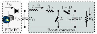
Figure 1: FC System under consideration.

We now replace (2) into (1a). The resulting equations (1) can be equivalently written as follows.

Fact 2

The FC System (1) can be represented by the dynamical system

$$Q\dot{x}=[J_{0}+J_{1}u-R]x+v_{1}I_{fc}(x_{1}),$$ (4)

where $u:=1-D$,

$$x :=\begin{bmatrix}v_{fc}\\ i_{L}\\ v_{o}\end{bmatrix},\;Q:=\begin{bmatrix}C_{fc}&0&0\\ 0&L&0\\ 0&0&C\end{bmatrix},\;J_{0}:=\begin{bmatrix}0&-1&0\\ 1&0&0\\ 0&0&0\end{bmatrix},$$

$$J_{1} :=\begin{bmatrix}0&0&0\\ 0&0&-1\\ 0&1&0\end{bmatrix},\;R:=\begin{bmatrix}0&0&0\\ 0&\theta_{r1}&0\\ 0&0&\theta_{r2}\end{bmatrix}.\;$$

For convenience, we also define the following vectors of parameters

$$\theta_{s}:=\begin{bmatrix}\theta_{s1}\\ \theta_{s2}\end{bmatrix},\;\theta_{r}:=\begin{bmatrix}\theta_{r1}\\ \theta_{r2}\end{bmatrix},\;\theta:=\begin{bmatrix}\theta_{r}\\ \theta_{s}\end{bmatrix}.$$

II-A Assignable equilibrium points

The control objective is to regulate the converter output voltage $x_{3}$ to some reference $x_{3}^{\star}>0$. According to that, the possible closed-loop equilibrium points are given in the following lemma.

Lemma 1

The assignable equilibrium points of (4) and the associated constant input are those values in the set

$$\mathcal{E} :=\left\{(x,u)\in\mathbb{R}^{4}:x_{1}=E_{oc}-\theta_{s1}x_{2}^{\theta_{s2}},\;p(x_{2},\theta)=0,\right.$$

$$\left.\hskip 42.67912ptx_{3}=x_{3}^{\star},\;u=x_{3}^{\star}\frac{(\theta_{r2}-\theta_{r1})x_{2}+x_{1}}{x_{2}^{2}+(x_{3}^{\star})^{2}}\right\},$$ (5)

where

$$p(x_{2},\theta):=\theta_{r1}x_{2}^{2}+\theta_{r2}(x_{3}^{\star})^{2}-x_{2}[E_{oc}-\theta_{s1}x_{2}^{\theta_{s2}}].$$

Proof:

Notice that (4) can be written in the affine form $Q\dot{x}=f(x)+g(x)u$ with

$$f(x):=(J_{0}-R)x,\;g(x):=\begin{bmatrix}0\\ -x_{3}\\ x_{2}\end{bmatrix}.$$ (6)

A full-rank left-hand annihilator of $g(x)$ is

$$g^{\perp}(x)=\begin{bmatrix}1&0&0\\ x_{1}&x_{2}&x_{3}\end{bmatrix}.$$

Therefore, at the equilibrium, the next relation holds

$$g^{\perp}(x)f(x)=\begin{bmatrix}I_{fc}-x_{2}\\ -\theta_{r1}x_{2}^{2}-\theta_{r2}x_{3}^{2}+x_{2}x_{1}\end{bmatrix}=0.$$ (7)

From (2), we obtain the voltage $x_{1}$ as

$$x_{1}=E_{oc}-\theta_{s1}I_{fc}^{\theta_{s2}}.$$ (8)

Employing the first equation in (7) produces the equilibrium value of $x_{1}$ showed in $\eqref{eqp}$. Replacing it into the second equation of (7), with $x_{3}=x_{3}^{\star}$, results in the second equation of $\mathcal{E}$. The control input $u$ in (1) is obtained using the left inverse as follows

$$u=-g^{+}(x)f(x).$$

$\Box\Box\Box$

II-B The full-information PI Passivity-based control

The proposition below introduces the PI-PBC for (4). As a first approach, we assume that all parameters in $\theta$ are known. An adaptive version of this controller is later presented, where the parameters are estimated online. For both the full-information PI-PBC and its adaptive extension, we assume the following.

Assumption 1

$x$ and $i_{fc}$ are measurable.

Lemma 2

Consider the FC System modeled by (4). Assume that all the parameters are known. Fix a desired, constant value for $x_{3}$ as $x_{3}^{\star}>0$ and compute from $\mathcal{E}$ the associated equilibrium vector $x^{\star}$. Consider the PI-PBC

$$\dot{x}_{c}= y_{N}(x),$$ (9a)

$$u= -K_{P}y_{N}(x)-K_{I}x_{c},$$ (9b)

where the input signal to the PI is defined as

$$y_{N}(x)= x_{2}^{\star}x_{3}-x_{3}^{\star}x_{2}.$$ (10)

For all positive constants $K_{p}$ and $K_{I}$ we have that all signals remain bounded ensuring the exponential convergence

$$\lim_{t\to\infty}\begin{bmatrix}x(t)\\ x_{c}(t)\end{bmatrix}=\begin{bmatrix}x^{\star}\\ x_{c}^{\star}\end{bmatrix},$$

where $x_{c}^{\star}=-K_{I}^{-1}u^{\star}$ with $u^{\star}\in\mathcal{E}$ the value of the control input at the equilibrium.

Proof:

We will first show that the system is stable. It follows modifying the proof of [18, Prop. 2] to include the presence of the term $I_{fc}$ and then invoke the monotonicity of Fact 1.

From (4), the error dynamics are

$$Q\dot{\tilde{x}}= \big{[}J_{0}+J_{1}(\tilde{u}+u^{\star})-R\big{]}(x^{\star}+\tilde{x})+v_{1}I_{fc}\pm v_{1}I_{fc}^{\star},$$

$$= (J_{0}+J_{1}u^{\star}-R)x^{\star}+v_{1}I_{fc}^{\star}+(J_{0}+J_{1}u-R)\tilde{x}$$

$$\hskip 105.2751pt+\tilde{u}J_{1}x^{\star}+v_{1}(I_{fc}-I_{fc}^{\star}),$$

$$= (J_{0}+J_{1}u-R)\tilde{x}+J_{1}x^{\star}\tilde{u}+v_{1}(I_{fc}-I_{fc}^{\star}),$$ (11)

where $\tilde{()}:=()-()^{\star}$, $I_{fc}^{\star}:=I_{fc}(x_{1}^{\star})$ and we use the equilibrium equation

$$(J_{0}+J_{1}u^{\star}-R)x^{\star}+v_{1}I_{fc}^{\star}=0,$$

to get the third identity. Now, we notice from (10) that the passive output $y_{N}$ may be written as

$$y_{N}=x^{\top}J_{1}x^{\star},$$

and moreover that $y_{N}(x^{\star})=0$, hence

$$y_{N}(x)=y_{N}(\tilde{x})=\tilde{x}^{\top}J_{1}x^{\star}.$$

Consider the Lyapunov function candidate for the system (9) and (11)

$$V(\tilde{x},\tilde{x}_{c})=\frac{1}{2}\tilde{x}^{\top}Q\tilde{x}+\frac{K_{I}}{2}\tilde{x}^{2}_{c}.$$

Its time derivative satisfies

$$\dot{V}= -\tilde{x}^{\top}R\tilde{x}+\tilde{u}y_{N}(\tilde{x})+K_{I}\tilde{x}_{c}y_{N}(\tilde{x})+\tilde{x}_{1}[I_{fc}-I_{fc}^{\star}].$$

From the inequality (3) in Fact 1, we have that

$$(x_{1}-x_{1}^{\star})[I_{fc}-I_{fc}^{\star}]=\tilde{x}_{1}[I_{fc}-I_{fc}^{\star}]\leq-\alpha\tilde{x}_{1}^{2}.$$

Therefore,

$$\dot{V}\leq -\tilde{x}^{\top}R\tilde{x}-\alpha\tilde{x}_{1}^{2}+\tilde{u}y_{N}(\tilde{x})+K_{I}\tilde{x}_{c}y_{N}(\tilde{x}),$$

$$= -\tilde{x}^{\top}R\tilde{x}-\alpha\tilde{x}_{1}^{2}+(u-u^{\star})y_{N}(\tilde{x})+K_{I}\tilde{x}_{c}y_{N}(\tilde{x}),$$

$$= -\tilde{x}^{\top}R\tilde{x}-\alpha\tilde{x}_{1}^{2}+\big{[}-K_{P}y_{N}(x)-K_{I}x_{c}$$

$$\hskip 85.35826pt+K_{I}x_{c}^{\star}\big{]}y_{N}(\tilde{x})+K_{I}\tilde{x}_{c}y_{N}(\tilde{x}),$$

$$= -\tilde{x}^{\top}R\tilde{x}-\alpha\tilde{x}_{1}^{2}-K_{P}y_{N}^{2}(\tilde{x}),$$

$$\leq -\tilde{x}^{\top}\mathrm{diag}(\alpha,\theta_{r1},\theta_{r2})\tilde{x}-K_{P}y_{N}^{2}(\tilde{x}),$$

$$\leq -\kappa|\tilde{x}|^{2}-K_{P}(\tilde{x}^{\top}g_{\star})^{2},$$

with $\kappa:=\mathrm{min}(\alpha,\theta_{r1},\theta_{r2})$ and, from (6), $g_{\star}:=g(x^{\star})=J_{1}x^{\star}$. We conclude that $\tilde{x}$ and $\tilde{x}_{c}$ are bounded. Consequently, $\tilde{u}$ and $u$ are also bounded. Moreover, the error dynamics of the closed loop are

$$Q\dot{\tilde{x}}= [R-J_{0}u+J_{1}]x-g_{\star}[K_{P}g_{\star}^{\top}\tilde{x}+K_{I}\tilde{x}_{c}]$$

$$\hskip 119.50148pt+v_{1}(I_{fc}-I_{fc}^{\star}),$$

$$\dot{\tilde{x}}_{c}= g_{\star}^{\top}\tilde{x},$$

The second step of this proof consists in demonstrating exponential stability as in [19, proposition 2]. For, we consider the following function

$$W(\tilde{x},\tilde{x}_{c})= V(\tilde{x},\tilde{x}_{c})+\epsilon K_{I}\tilde{x}^{\top}g_{\star}\tilde{x}_{c},$$

$$= \frac{1}{2}\chi^{\top}\begin{bmatrix}Q&\epsilon K_{I}g_{\star}\\ \epsilon K_{I}g_{\star}^{\top}&K_{I}\end{bmatrix}\chi,$$

where $\chi:=\mathrm{col}(\tilde{x},\tilde{x}_{c})$ and a constant $\epsilon>0$. The function $W$ is positive definite iff

$$Q-\epsilon^{2}K_{I}g_{\star}g_{\star}^{\top}>0.$$ (12)

The time derivative of $W$ is

$$\dot{W}= \dot{V}+\epsilon K_{I}\tilde{x}^{\top}g_{\star}\dot{\tilde{x}}_{c}+\epsilon K_{I}\tilde{x}_{c}g_{\star}^{\top}\dot{\tilde{x}},$$

$$\leq -\kappa|\tilde{x}|^{2}-K_{P}(\tilde{x}^{\top}g_{\star})^{2}+\epsilon K_{I}(\tilde{x}^{\top}g_{\star})^{2}+\epsilon K_{I}\tilde{x}_{c}g_{\star}^{\top}\dot{\tilde{x}},$$

$$= -\kappa|\tilde{x}|^{2}-(K_{P}-\epsilon K_{I})(\tilde{x}^{\top}g_{\star})^{2}$$

$$\hskip 14.22636pt+\epsilon K_{I}\tilde{x}_{c}\big{(}g_{\star}^{\top}Q^{-1}[J_{o}u+J_{1}-R]$$

$$\hskip 14.22636pt-K_{P}g_{\star}^{\top}Q^{-1}g_{\star}g_{\star}^{\top}\big{)}\tilde{x}-\epsilon K_{I}^{2}g_{\star}^{\top}Q^{-1}g_{\star}\tilde{x}_{c}^{2},$$

$$= -\kappa|\tilde{x}|^{2}-(K_{P}-\epsilon K_{I})(\tilde{x}^{\top}g_{\star})^{2}$$

$$\hskip 56.9055pt-\epsilon\tilde{x}_{c}s^{\top}\tilde{x}-\epsilon K_{I}^{2}g_{\star}^{\top}Q^{-1}g_{\star}\tilde{x}_{c}^{2},$$

where, to obtain the expression in the third line, we used the fact that the product $g_{\star}^{\top}\dot{\tilde{x}}$ is

$$g_{\star}^{\top}\dot{\tilde{x}},= g_{\star}^{\top}Q^{-1}\left\{[J_{0}u+J_{1}-R]\tilde{x}-g_{\star}[K_{p}g_{\star}^{\top}\tilde{x}+K_{I}\tilde{x}_{c}]\right.$$

$$\hskip 133.72786pt\left.+v_{1}(I_{fc}-I_{fc}^{\star})\right\},$$

with

$$g_{\star}^{\top}Q^{-1}v_{1}(I_{fc}-I_{fc}^{\star})=0.$$ (13)

Also, to obtain the expression in the forth line, we defined

$$s^{\top}:=-K_{I}g_{\star}^{\top}Q^{-1}[J_{0}u+J_{1}-R]+K_{I}K_{p}g_{\star}^{\top}Q^{-1}g_{\star}g_{\star}^{\top},$$

The inequality above can be written in the matrix form

$$\dot{W}\leq-\chi^{\top}M\chi,$$ (14)

where

$$M:=\begin{bmatrix}\kappa I_{3}+(K_{P}-\epsilon K_{I})g_{\star}g_{\star}^{\top}&\frac{\epsilon}{2}s\\ \frac{\epsilon}{2}s^{\top}&\epsilon K_{I}^{2}g_{\star}^{\top}Q^{-1}g_{\star}\end{bmatrix}.$$

The matrix $M$ is positive definite iff

$$\kappa I_{3}+ K_{p}g_{\star}g_{\star}^{\top}-\epsilon\left[K_{I}g_{\star}g_{\star}^{\top}\right.$$

$$\hskip 71.13188pt\left.+\frac{1}{4K_{I}^{2}}s(g_{\star}^{\top}Q^{-1}g_{\star})^{-1}s^{\top}\right]>0.$$ (15)

We conclude the proof noting that there exists a sufficiently small constant $\epsilon>0$ satisfying (12) and (II-B). Exponential convergence follows [khalil, Theorem 4.10]. $\Box\Box\Box$

III Main result

III-A Estimation of $\theta$

An estimator of $\theta$ is a dynamical system of the form

$$\dot{\eta}(t)= \chi_{\eta}(t,\eta(t),x(t)),$$ (16)

$$\hat{\theta}(t)= \chi_{\theta}(t,\eta(t),x(t)),$$

where $\hat{\theta}$ is the estimate of $\theta$. Such that

$$\lim_{t\to\infty}\hat{\theta}(t)=\theta.$$ (17)

Here below, an estimation algorithm for $\theta$ in (4) is proposed. This combines two already reported estimation approaches: the I&I technique [14] and the gradient-descent estimator [15] techniques. More precisely, the I&I approach is employed to estimate $\theta_{r}$ whereas the gradient-descent estimator is implemented to identify $\theta_{s}$.

The next lemma introduces a linear regression equation (LRE) obtained from the polarization curve (2). This LRE is part of the estimator equations introduced below. The proof can be found in [16, Lemma 4].

Lemma 3

Consider the algebraic relation in (2) with $E_{oc}$ as a known parameter. Then, the next LRE holds

$$Y(t)=\phi(t)\theta_{s2},$$ (18)

where

$$Y =\mathcal{F}\{\ln(E_{oc}-x_{1})\},$$

$$\phi =\mathcal{F}\{\ln(i_{fc})\},$$

and the operator $\mathcal{F}\{\cdot\}$ is the stable, LTI filter

$$\mathcal{F}:=\frac{\lambda p}{p+\lambda},\;\lambda>0.$$

Before introducing the estimation algorithm, the following excitation assumption is in order.

Assumption 2

$x_{2},x_{3}$ and $\phi\not\in\mathcal{L}_{2}$.

Proposition 1 (Parameter estimator)

Let the estimator (16) be composed of the following dynamics:

• (Estimation of $\theta_{s}$) The gradient-descent estimator:

  $$\dot{\hat{\theta}}_{s2}= \gamma\phi(Y-\phi\hat{\theta}_{s2}),$$ (19a)

  $$\hat{\theta}_{s1}= (E_{oc}-x_{1})i_{fc}^{-\hat{\theta}_{s2}},$$ (19b)

  for a positive gain $\gamma.$

• (Estimation of $\theta_{r}$) The I&I estimator:

  $$\dot{r}_{1}= -k_{1}x_{2}\left(-x_{1}-\frac{1}{2}k_{1}Lx_{2}^{3}+r_{1}x_{2}+x_{3}u\right),$$ (20a)

  $$\dot{r}_{2}= -k_{2}x_{3}\left(-x_{2}u-\frac{1}{2}k_{2}Cx_{3}^{3}+r_{2}x_{3}\right)\;,$$ (20b)

  $$\hat{\theta}_{r1}= -{k_{1}\over 2}Lx^{2}_{2}+r_{1},$$ (20c)

  $$\hat{\theta}_{r2}= -{k_{2}\over 2}Cx^{2}_{3}+r_{2},$$ (20d)

  where $k_{1}$ and $k_{2}$ are positive gains.

Fulfillment of Assumption 2 ensures that the estimation error, defined as $e:=\hat{\theta}-\theta$, is bounded and

$$\lim_{t\to\infty}e(t)=0,$$ (21)

Proof:

The gradient-descent estimator in (19a) is a standard estimation algorithm. Its error $e_{s2}$, defined as $e_{s2}:=\hat{\theta}_{s2}-\theta_{s2}$, has the following dynamic

$$\dot{e}_{s2}=-\gamma\phi^{2}e_{s2}.$$

Assumption 2 implies the convergence of $e_{r2}$. Moreover, using (2) with $\hat{\theta}_{s2}$ instead of the actual parameter value $\theta_{s2}$, it is possible to obtain an estimate of $\theta_{s1}$ as in (19b).

We now prove the convergence of the I&I estimator. The estimation error $e_{r1}$, defined as $e_{r1}:=\hat{\theta}_{r1}-\theta_{r1}$, has the following dynamics

$$\dot{e}_{r1}= \dot{r}_{1}-k_{1}Lx_{2}\dot{x}_{2},$$

$$= k_{1}x_{2}(x_{1}-r_{1}x_{2}+{k_{1}\over 2}Lx^{3}_{2}-x_{3}u)$$

$$\hskip 51.21504pt-k_{1}x_{2}[-(\hat{\theta}_{r1}-\tilde{\theta}_{r1})x_{2}+x_{1}-x_{3}u],$$

$$= -k_{1}x_{2}(x_{3}u+\hat{\theta}_{r1}x_{2})$$

$$\hskip 51.21504pt-k_{1}x_{2}[-(\hat{\theta}_{r1}-\tilde{\theta}_{r1})x_{2}-x_{3}u],$$

$$= -k_{1}x_{2}^{2}\tilde{\theta}_{r1},$$

where (20c) was used to obtain the third equality. With a similar procedure, the estimation error $e_{r2}:=\hat{\theta}_{r2}-\theta_{r2}$, evolves according to the following dynamics

$$\dot{{e}}_{r2}= \dot{r}_{2}-k_{2}Cx_{3}\dot{x}_{3},$$

$$= k_{2}x_{3}[x_{2}u-r_{2}x_{3}+{k_{2}\over 2}Cx^{3}_{3}]$$

$$\hskip 42.67912pt-k_{2}x_{3}[-(\hat{\theta}_{r2}-\tilde{\theta}_{r2})x_{3}+x_{2}u],$$

$$= k_{2}x_{3}(x_{2}u-\hat{\theta}_{r2}x_{3})-k_{2}x_{3}[-(\hat{\theta}_{r2}-\tilde{\theta}_{r2})x_{3}+x_{2}u],$$

$$= -k_{2}x_{3}^{2}\tilde{\theta}_{r2}.$$

Again, since $x_{2}$ and $x_{3}\not\in\mathcal{L}_{2}$ by assumption, $e_{r1}$ and $e_{r2}$ converge to zero.

$\Box\Box\Box$

III-B The proposed adaptive PI-PBC

The full-information PI-PBC of Lemma 2 depends on the equilibrium points. When parameters are available, the equilibrium are numerically computed by a root-finding procedure applied to the equilibrium equations of $\mathcal{E}$. On the other hand, when these parameters are unknown, a parameter estimation has to be performed. An estimate of the equilibrium point can be carried out by solving the equations of (1) that result from replacing the actual parameters with their estimate $\hat{\theta}$. In other words, for a given $\hat{\theta}$, the estimate of the equilibrium point, denoted as $\hat{x}^{\star}$, belongs to the set

$$\hat{\mathcal{E}}:= \left\{x\in\mathbb{R}^{3}:x_{1}=E_{oc}-\hat{\theta}_{s1}x_{2}^{\hat{\theta}_{s2}}\right.,$$

$$\hskip 85.35826pt\;\left.p(x_{2},\hat{\theta})=0,~{}x_{3}=x_{3}^{\star}\right\},$$ (22)

where the mapping $p(\cdot,\cdot)$ has been defined in (1). It can be noted that finding the elements in $\hat{\mathcal{E}}$ involves the search of a root of $p(x_{2},\hat{\theta})=0$, which in principle, may not exist. In this sense, the Implicit Function theorem (see, for example, [20, Section A.1]) provides sufficient conditions for the existence of solutions of this equation.

Lemma 4

Let $x^{\star}\in\mathcal{E}$ be an assignable equilibrium point of (4) and assume that

$$2{\theta}_{r1}x_{2}^{\star}+(\theta_{s2}+1)\theta_{s1}(x_{2}^{\star})^{{\theta}_{s2}}-E_{oc}\not=0.$$ (23)

Then, there exist $\varepsilon>0$ and $\hat{x}_{2}^{\star}\in\mathbb{R}$ such that for any $\hat{\theta}$ satisfying $|\hat{\theta}-\theta|<\varepsilon$, it holds that

$$p(\hat{x}_{2}^{\star},\hat{\theta})=0.$$

Namely, a solution of the second equation in (22) exists.

Proof:

The derivative of $p(x_{2},\hat{\theta})$ with respect to $x_{2}$ is

$$\frac{dp}{dx_{2}}(x_{2},\hat{\theta})= 2\hat{\theta}_{r1}x_{2}+(\hat{\theta}_{s2}+1)\hat{\theta}_{s1}x_{2}^{\hat{\theta}_{s2}}-E_{oc}.$$

We then evaluate the last expression in $(x_{2},\hat{\theta})=(x_{2}^{\star},\theta)$. The resulting equation is prevented from being zero by condition (23). Consequently, the Implicit Function theorem guarantees the existence of a smooth function $h(\hat{\theta})$, mapping each $\hat{\theta}$ in a neighborhood of $\theta$ to a point $\hat{x}_{2}^{\star}$ in a neighborhood of $x_{2}^{\star}$ such that

$$p(h(\hat{\theta}),\hat{\theta})=0.$$

$\Box\Box\Box$

We are now in position to state our main contribution which is summarized by the next proposition that introduces an adaptive PI-PBC (API-PBC) for (4).

Proposition 2 (Adaptive PI-PBC)

Consider the closed loop of the FC System modeled by eqs. (4), the parameter estimator (19)-(20) and the API-PBC

$$u= -K_{p}\hat{y}_{N}-K_{I}x_{c},$$ (24a)

$$\dot{x}_{c}= \hat{y}_{N},$$ (24b)

where $\hat{y}_{N}(x):=\hat{x}_{2}^{\star}x_{3}-x_{3}^{\star}x_{2}$, $K_{p}$ and $K_{I}$ are positive tunning gains, $x_{3}^{\star}>0$ is the voltage setpoint and $\hat{x}_{2}^{\star}$ is the estimation of $x_{2}^{\star}$ computed from (22). Suppose that (23) together with Assumptions 1 and 2 are satisfied. Then, all signals remain bounded and the equilibrium point $(\hat{\theta},x,x_{c})=(\theta,x^{\star},-K_{I}^{-1}u^{\star})$ is asymptotically stable.

Proof:

Note that the adaptive PI-PBC (24) depends on the estimate $\hat{x}^{\star}_{2}$. It can be represented by the function $u=\beta(x,\hat{x}_{2}^{\star},x_{3}^{\star},x_{c})$. We write $\hat{x}_{2}^{\star}$ as the addition $\hat{x}^{\star}_{2}=x^{\star}_{2}+\delta$, where $\delta:=\hat{x}^{\star}_{2}-x^{\star}_{2}$ is the deviation of the estimation of the equilibrium with respect to its actual value. The dynamics of the FC System in a closed loop with the controller has the form

$$\dot{x}= f_{cl}(x,\beta(x,x^{\star}_{2}+\delta,x_{3}^{\star},x_{c})),$$ (25)

$$\dot{x}_{c}= g_{cl}(x,x^{\star}_{2}+\delta,x_{3}^{\star}).$$

Setting $\delta=0$ in (25) results in the system of Lemma 2 which has been proven to be exponentially stable. On other hand, from Proposition 1, $\hat{\theta}$ is bounded and converges to $\theta$. From Lemma (4), $\hat{x}_{2}^{\star}$, a root of $p(x_{2},\hat{\theta})=0$, is guaranteed to exist in a neighborhood of $\theta$. The error $\delta$ is then bounded and $\delta\to 0$ as $\hat{\theta}\to\theta$. Now, in virtue of [21, Corollary 9.2], the equilibrium point $(x,x_{c})=(x^{\star},-K_{I}^{-1}u^{\star})$ of (25) is asymptotically stable. $\Box\Box\Box$

IV Experimental results

Experimental validation of the API-PBC for output voltage regulation is performed with the test bench shown in Fig. 2. It consists of: 1) a data acquisition system dSPACE-DS1104, 2) a fully automated 1.2 kW Nexa$\textregistered$ PEMFC power stack, 3) a 250 W boost converter prototype, 4) a resistive load, 5) a function generator, 6) an oscilloscope, and 7) a conditioning circuit boards for voltage and current sensing. The dSPACE is configured with the Euler numerical solver and a fixed-time step of 100 $\mu$s. The nominal values of the experimental setup and the gain values are shown in Table I. The open-circuit voltage of the PEMFC was manually measured before starting the experimentation session. It reached a value of $E_{oc}=38.84$ V. An implementation block diagram of the API-PBC is illustrated in Fig. 3. In this figure, the block labeled as “Computation of equilibria” receives the parameter estimate $\hat{\theta}$. From this vector, an estimation of the equilibrium point $\hat{x}^{\star}_{2}\in\hat{\mathcal{E}}$ is computed via the Newton-Raphson Method. That is, a numerical solution of

$$p(x_{2},\hat{\theta})=0,$$

is online found, for each value $\hat{\theta}$ given by the estimation algorithm.

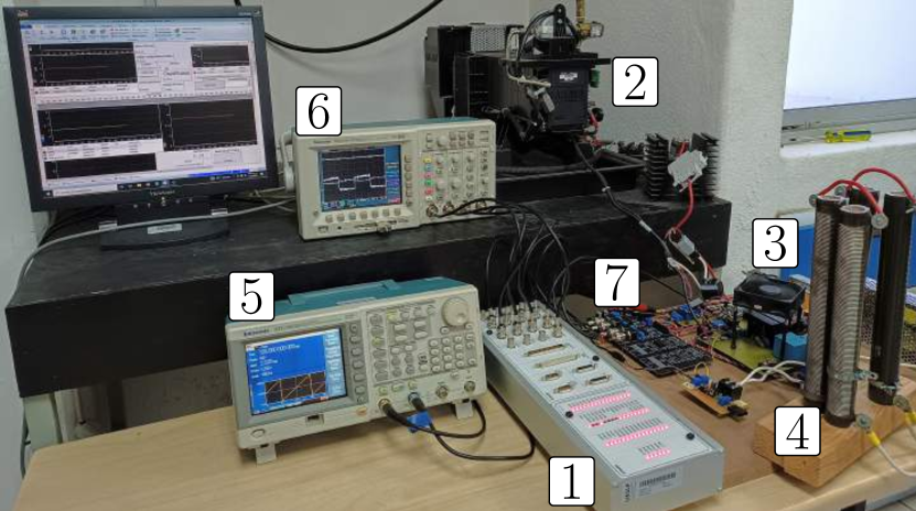
Figure 2: Experimental testbench for the FC System with the Nexa® PEMFC power stack.

Parameters	Nominal value	Unit	Gains	Values
$C$	136	$\mu$F	$k_{1}$	2.00
$C_{fc}$	5.19	mF	$k_{2}$	2.00
$L$	38.6	$\mu$H	$K_{P}$	19.0$\times 10^{-6}$
$\theta_{r1}$	8.30	m$\Omega$	$K_{I}$	0.28
$\theta_{r2}$	47.1 or 94.2	mS	$\lambda$	4.50
$f_{sw}$	100	kHz	$\gamma$	3.00
$E_{oc}$	38.84	V

TABLE I: Parameters and gains used during experimental validation.

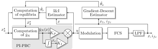
Figure 3: Implementation diagram of the API-PBC

The correct performance of the API-PBC for output voltage regulation is verified against two standard and real-life scenarios. First, pulsating changes are considered in the voltage reference while the load is kept constant. Second, pulsating changes are considered in the load while the voltage reference is kept constant. The results of both scenarios are detailed below.

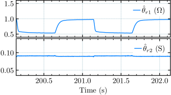
(a) Online estimations with voltage reference changes.

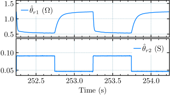
(b) Online estimations with load changes.

Figure 4: Experimental results of the online estimation of the parasitic resistance of the inductor and the load conductance through I&I.

IV-1 Pulsating voltage reference changes

The voltage reference pulsates at 1.0 Hz from 48.0 V to 38.0 V while the load is kept constant at 90.15 mS. This scenario is performed from 141.7 s to 208.7 s. In Figs. 5, 4(a), and 7 we present the dynamic response of the system states, PEMFC current, control signal, and online estimations. It is important to reiterate that voltage regulation requires a suitable estimation of the current reference $\hat{x}_{2}^{\star}$, which requires the online estimations of (19)-(20) and is the numerical solution of the polynomial of (1). Inspection of Figs. 5(a) and 5(b) indicate that each state is tracking its reference until the voltage reference changes, causing a significant error in the output voltage. After this, in less than 80 ms the output voltage is again tightly regulated and the other states track their references. This implies that a suitable current $\hat{x}_{2}^{\star}$ is obtained through the self-tuning of the estimator and the solution of (1). Moreover, it is also observed that the PEMFC voltage reference is being appropriately estimated with the power function model and values taken by the control signal are achievable. As can be seen in Fig. 4(a), the estimate $\hat{\theta}_{r1}$ is not constant, since it captures not only the parasitic resistance of the inductor, but also unmodeled resistances such as diode and switch ON resistances, and capacitor equivalent series and leakage resistances. On the other hand, as expected, the estimate $\hat{\theta}_{r2}$ has no significant variations. The online estimation of $\hat{\theta}_{s}$ can be observed in Fig. 7. As mentioned previously, only $\hat{\theta}_{s2}$ is estimated online. This estimation takes a minimum of 0.680 and a maximum of 0.997 during this scenario. Calculating average values of the data, it is obtained $\bar{\hat{\theta}}_{s}=(0.984,\;0.865)$. Observe that this estimation has small variations due to the hysteresis phenomenon exhibited by the PEMFC, although this fact is of no consequence for the estimation of the current reference $\hat{x}_{2}^{\star}$ or the PEMFC voltage $\hat{x}_{1}^{\star}$. Finally, the resulting steady-state values are $\hat{x}^{\star}=(33.32\;\mathrm{V}$, $7.11\;\mathrm{A},48.0\;\mathrm{V})$ with $\hat{\theta}_{r}^{\star}=(542.31\;\mathrm{m}\Omega,90.85\;\mathrm{mS})$ and $\hat{x}^{\star}=(35.75\;\mathrm{V},4.05\;\mathrm{A},38.0\;\mathrm{V})$ with $\hat{\theta}_{r}^{\star}=(978.28\;\mathrm{m}\Omega,89.50\;\mathrm{mS})$.

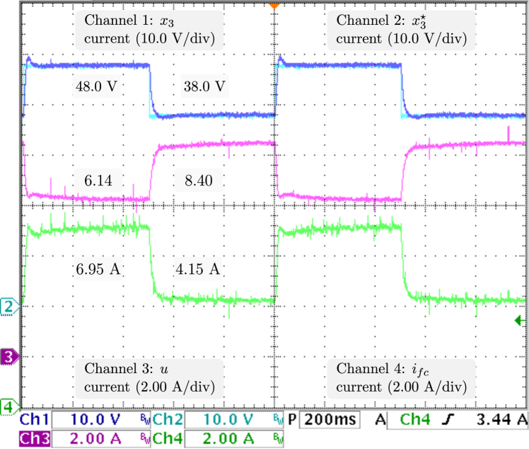
(a) From top to bottom: $x_{3}$ (Ch1), $x_{3}^{\star}$ (Ch2), $u$ (Ch3), and $i_{fc}$ (Ch4).

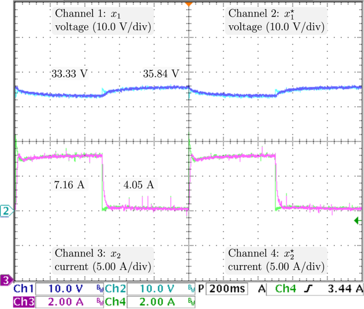
(b) From top to bottom: $x_{1}$ (Ch1), $x_{1}^{\star}$ (Ch2), $x_{2}$ (Ch3), and $x_{2}^{\star}$ (Ch4).

Figure 5: Experimental results of the output voltage regulation under pulsating voltage reference changes at 1 Hz. The resulting equilibria are $x^{\star}=($33.32 V, 7.11 A, 48.0 V$)$ and $x^{\star}=($35.75 V, 4.05 A, 38.0 V$)$.

IV-2 Pulsating load changes

The load pulsates at 1.0 Hz from 90.87 mS to 46.54 mS while the voltage reference remains at 48.0 V. This scenario is performed from 219.9 s to 278.4 s. In Figs. 6, 4(b), and 7, we present the dynamic response of the system states, PEMFC current, control signal, and online estimations. As we can see from Figs. 6(a), 6(b), and 4(b), each state is tracking its reference until the load changes, which produces a noticeable error in the output voltage. Then, in less than 120 ms, the output voltage is again tightly regulated and the other states track their references. This implies that a suitable current $\hat{x}_{2}^{\star}$ is obtained through the self-tuning of the hybrid estimator and the solution of (1). Also, similar to the previous scenario, the PEMFC voltage is properly estimated and the values taken by the control signal are achievable. Similar to the previous scenario, we observe from Fig. 4(b) that $\hat{\theta}_{r1}$ has smooth variations, while the estimation $\hat{\theta}_{r2}$ is done quickly. The online estimation of $\hat{\theta}_{s}$ can be found in Fig. 7. In this scenario, the online estimation $\hat{\theta}_{s2}$ takes a minimum of 0.600 and a maximum of 1.167. Computing average data values $\bar{\theta}_{s}^{\star}=(0.999,\;0.921)$. Note that in this scenario we also see variations in the estimates. Finally, the resulting steady-state values are $\hat{x}^{\star}=(33.12\;\mathrm{V},7.15\;\mathrm{A},48.0\;\mathrm{V})$, with $\hat{\theta}_{r}^{\star}=(536.18\;\mathrm{m}\Omega,90.87\;\mathrm{mS})$ and $\hat{x}^{\star}=($36.29$\;\mathrm{V}$, 3.31$\;\mathrm{A},48.0\;\mathrm{V})$, with $\hat{\theta}_{r}^{\star}=(1.22\;\Omega,46.54\;\mathrm{mS})$.

Lastly, in Fig. 8 we compare experimental “data” obtained of more than ten thousand $(i_{fc},v_{fc})$ measurements with a model of the polarization curve for each scenario, “Scenario 1” and “Scenario 2”. These models are computed using the measured $E_{oc}$ and their respective averaged $\bar{\hat{\theta}}_{s}$. As we can see, the hysteresis phenomena is observed in the experimental data, and is worth mentioning that modeling this complex dynamics is beyond the scope of this study. Nevertheless, in steady-state operation the power model “Scenario 1” fits the central section of the hysteresis band, meanwhile the power model of “Scenario 2” fits only at low currents. It should be noted that average values $\bar{\hat{\theta}}_{s}$ obtained off-line were used only for the comparison. Recall that online estimation of $\hat{\theta}_{s}$, as shown in Fig. 7, is given to the API-PBC and during both scenarios a suitable estimation of the inductor current and PEMFC voltage equilibrium points are obtained.

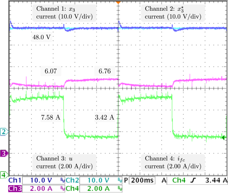
(a) From top to bottom: $x_{3}$ (Ch1), $x_{3}^{\star}$ (Ch2), $u$ (Ch3), and $i_{fc}$ (Ch4).

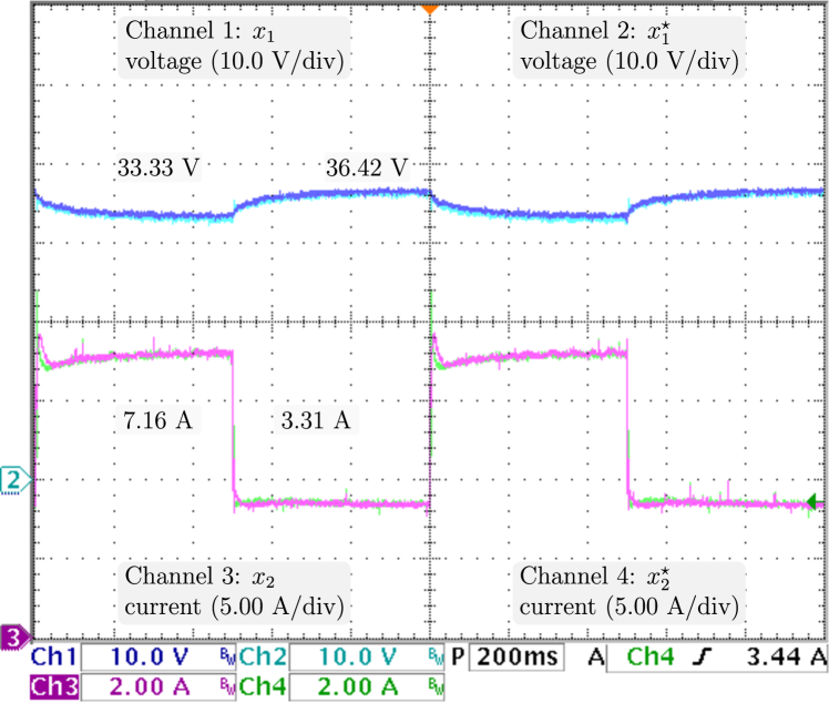
(b) From top to bottom: $x_{1}$ (Ch1), $x_{1}^{\star}$ (Ch2), $x_{2}$ (Ch3), and $x_{2}^{\star}$ (Ch4).

Figure 6: Experimental results of the output voltage regulation under pulsating voltage reference changes at 1 Hz. The resulting equilibria are $x^{\star}=($33.12 V, 7.15 A, 48.0 V$)$ and $x^{\star}=($36.29 V, 3.31 A, 48.0 V$)$.

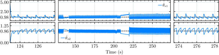
Figure 7: Experimental results of the online PEMFC parameters estimations through gradient-descend.

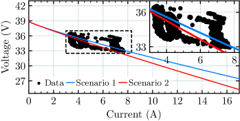
Figure 8: Comparison of experimental “Data” with the polarization curve model computed using the average values for the estimations in both scenarios, “Scenario 1” and “Scenario 2”.

V Conclusions

We derived a PI-PBC for the fuel-cell system of eq. (4). The resulting controller has the same structure as that in [18] in spite of the fact that the class of systems to which the FC System belongs is not the one therein addressed. An adaptive version of the approach is afterward introduced, based on an indirect output voltage regulation control scheme. Parameter estimation is carried out using the I&I and the gradient-descent online algorithms.

As a final comment, we notice that system (4) can be generalized to systems having the form

$$Q\dot{x}=[J_{0}-R]x+\sum_{i=1}^{m}g_{i}(x)u_{i}+d(x),$$ (26)

where $d:\mathbb{R}^{n}\to\mathbb{R}^{n}$ and

$$g_{i}(x)=J_{i}x+b_{i}.$$

Clearly, (26) enlarges the family of systems considered in [18]. On the other hand, we identify that the two key features that make possible to apply the PI-PBC (and the stability analysis) presented in [19] and [18] to the system (4) are the monotonicity property (3) and (13). The first feature allows, together with the matrix $R$, to have dissipation. The second feature yields the quadratic form of (14).

In this manner, an immediate attempt to extend Lemma 2 would lead to the imposition on system (26) of the following two (restrictive) conditions:

1. The $\ell$-th entry of vector $d$ is the mapping $d_{\ell}(x_{\ell})$, which satisfies strong monotonicity. That is, for any scalars $y$ and $z$ there exists a non-negative constant $\alpha_{\ell}$ such that

   $$(y-z)^{\top}\big{[}[-d_{\ell}(y)]-[-d_{\ell}(z)]\big{]}\geq\alpha_{\ell}|y-z|^{2},$$

   with $\ell=1,\cdots,n$.

2. For $y$ and $z\in\mathbb{R}^{n}$ and $i=1,\cdots,m$,

   $$g_{i}^{\top}(y)Q^{-1}d(z)=0.$$

Future work is oriented to the relaxation of conditions C1 and C2 in order for the PI-PBC to be applied.

References

• [1] K. Jiao, J. Xuan, Q. Du, Z. Bao, B. Xie, B. Wang, Y. Zhao, L. Fan, H. Wang, Z. Hou, S. Huo, N. P. Brandon, Y. Yin, and M. D. Guiver, “Designing the next generation of proton-exchange membrane fuel cells,” Nature, vol. 595, pp. 361–369, 7 2021.
• [2] Y. Wang, D. F. R. Diaz, K. S. Chen, Z. Wang, and X. C. Adroher, “Materials, technological status, and fundamentals of pem fuel cells – a review,” Materials Today, vol. 32, pp. 178–203, 1 2020.
• [3] E. Ogungbemi, T. Wilberforce, O. Ijaodola, J. Thompson, and A. Olabi, “Selection of proton exchange membrane fuel cell for transportation,” International Journal of Hydrogen Energy, vol. 46, pp. 30 625–30 640, 8 2021.
• [4] D. A. J. Dicks, Andrew; Rand, Fuel cell systems explained, third edition ed.   Wiley, 2018.
• [5] A. Shahin, M. Hinaje, J.-P. Martin, S. Pierfederici, S. Rael, and B. Davat, “High voltage ratio dc–dc converter for fuel-cell applications,” IEEE Transactions on Industrial Electronics, vol. 57, pp. 3944–3955, 12 2010.
• [6] M. Hilairet, M. Ghanes, O. Béthoux, V. Tanasa, J.-P. Barbot, and D. Normand-Cyrot, “A passivity-based controller for coordination of converters in a fuel cell system,” Control Engineering Practice, vol. 21, pp. 1097–1109, 8 2013.
• [7] R. Cisneros, R. Ortega, C. Beltrán, D. Langarica-Córdoba, and L. Díaz, “Output voltage regulation of a fuel cell/boost converter system: A PI-PBC approach,” International Journal of Adaptive and Control Signal Processing, vol. 9, no. 39, pp. 286–295, 2023.
• [8] Y. A. Zúñiga-Ventura, J. Leyva-Ramos, L. H. Díaz-Saldiema, I. A. Díaz-Díaz, and D. Langarica-Córdoba, “Nonlinear voltage regulation strategy for a fuel cell/supercapacitor power source system,” in IECON 2018 - 44th Annual Conference of the IEEE Industrial Electronics Society, 2018, pp. 2373–2378.
• [9] Y. Xing, J. Na, and R. Costa-Castello, “Real-time adaptive parameter estimation for a polymer electrolyte membrane fuel cell,” IEEE Transactions on Industrial Informatics, vol. 15, pp. 6048–6057, 11 2019.
• [10] H. Chaoui, M. Kandidayeni, L. Boulon, S. Kelouwani, and H. Gualous, “Real-time parameter estimation of a fuel cell for remaining useful life assessment,” IEEE Transactions on Power Electronics, vol. 36, pp. 7470–7479, 7 2021.
• [11] Y. Furukawa, Y. Shibata, H. Eto, I. Colak, and F. Kurokawa, “Static analysis of a digital peak current mode control dc–dc converter using current–frequency conversion,” IEEE Transactions on Power Electronics, vol. 37, no. 7, pp. 7688–7704, 2022.
• [12] Y. A. Zúñiga Ventura, D. Langarica-Córdoba, J. Leyva-Ramos, L. Díaz-Saldierna, and V. Ramírez-Rivera, “Adaptive backstepping control for a fuel cell/boost converter system,” IEEE Journal of Emerging and Selected Topics in Power Electronics, vol. 6, pp. 686–695, 2018.
• [13] C. Beltrán, L. Díaz-Saldierna, D. Langarica-Córdoba, and P. Martínez-Rodríguez, “Passivity-based control for output voltage regulation in a fuel cell/boost converter system,” Micromachines, vol. 14, p. 187, 2023.
• [14] A. Astolfi, D. Karagiannis, and R. Ortega, Nonlinear and adaptive control with applications.   Berlin: Springer-Verlag, 2008.
• [15] S. Sastry and M. Bodson, Adaptive control: Stability, convergence and robustness.   Dover Publications, 2011.
• [16] C. Beltrán, A. Bobsov, R. Ortega, D. Langarica-Córdoba, R. Cisneros, and L. Díaz, “Online parameter estimation of the polarization curve of a fuel cell with guaranteed convergence properties: Theoretical and experimental results,” IEEE Transactions on Industrial Electronics, vol. 54, no. 2, pp. 286–295, 2024.
• [17] A. Pavlov, A. Pogromsky, N. van de Wouw, and H. Nijmeijer, “Convergent dynamics, a tribute to Boris Pavlovich Demidovich,” System & Control Letters, vol. 52, no. 3-4, pp. 257–261, 2004.
• [18] M. Hernández-Gómez, R. Ortega, F. Lamnabhi-Lagarrigue, and G. Escobar, “Adaptive PI stabilization of switched power converters,” IEEE Transactions on Control System Technology, vol. 18, no. 3, pp. 688–698, 2010.
• [19] D. Zonetti, G. Bergna-Díaz, R. Ortega, and N. Monshizadeh, “PID passivity-based control of power converters,” International Journal on Robust and Nonlinear Control, vol. 32, no. 1, pp. 1769–1795, 2022.
• [20] A. Isidori, Nonlinear Systems, 2nd ed.   Springer, 1994.
• [21] W. Terrell, Stability and stabilization: An introduction, 1st ed.   Princeton University Press, 2009.