Dissipation rates from experimental uncertainty

Abstract

Experimental uncertainty prompted the early development of the quantum uncertainty relations now known as speed limits. However, it has not yet been a part of the development of thermodynamic speed limits on dissipation. Here, we predict the maximal rates of heat and entropy production using experimentally accessible uncertainties in a thermodynamic speed limit. Because these rates can be difficult to measure directly, we reparametrize the speed limit to predict these observables indirectly from quantities that are readily measurable with experiments. From this transformed speed limit, we identify the resolution an experiment will need to upper bound nonequilibrium rates. Without models for the dynamics, these speed limit predictions agree with calorimetric measurements of the energy dissipated by a pulled Brownian particle and a microtubule active gel, validating the approach and suggesting potential for the design of experiments.

Introduction.– Dissipation rates determine the efficiency of biological materials [1, 2] and are a critical feature in the design of active synthetic systems [3, 4, 5, 6, 7, 8, 9, 10]. For example, it is now possible to create active cytoskeletal materials in a nonequilibrium state consuming chemical energy and dissipating heat at picowatt rates [11]. Recently, it has become possible to measure these rates across length and time scales with sophisticated calorimetry techniques [12], which can be interpreted with models for the rate limiting reactions and direct observations of dissipative degrees of freedom in space and time, e.g., with high-resolution microscopy [13]. Theoretically-grounded estimates of nonequilibrium observables could guide this experimentation on functional materials and their design [14, 15, 16]. However, it is theoretically challenging to predict dissipation rates and other thermodynamic costs a priori from available experimental data (e.g., concentrations, particle positions) without reliable models of the dynamics.

Surveying stochastic thermodynamics [17, 18], the thermodynamic speed limit [19, 20] set by the Fisher information [21, 22, 23] $I_{F}=\tau^{-2}$ has potential for direct application to experiments. This single timescale upper bounds the rate of heat, entropy production, dissipated work, chemical work [24, 20] and, more recently, mechanical work [25, 26]. For example, a system that dissipates energy as heat with a rate $\dot{Q}$ and is subject to energy fluctuates with a standard deviation $\Delta\epsilon$ has the speed limit [20] on the speed of heat flow,

$$\tau_{Q}^{-1}:=\frac{|\dot{Q}|}{\Delta\epsilon}\leq\sqrt{I_{F}}=:\tau^{-1},$$ (1)

even if work is done on or by the system . Speed limits on dissipation rates are now known in quantum [28, 29, 30], classical deterministic [31, 32], and stochastic [33, 34, 35, 20] dynamics. Alternative approaches to infer dissipation, such as the thermodynamic uncertainty relation [36, 37, 38, 39, 40, 41, 42, 43, 44, 45] and its extensions [46, 47], estimate dissipation through the statistics of currents [48], while others use optimization methods and transition rates [49, 50] or waiting times [49, 51]. However, these approaches give lower bounds on entropy production rates and not necessarily explicit functions of easily measurable observables or estimates of the energy dissipated as heat. By contrast, estimates of the Fisher information in Eq. (1) would give upper bounds on the maximum rate of dissipation of entropy, heat, and free energy.

The fluctuations and Fisher information also create potential for using experimental measures of uncertainty as input for the thermodynamic speed limit. Historically, the analysis of uncertainty was important in Heisenberg’s arguments for quantum mechanical uncertainty relations. The time-energy uncertainty relation he proposed is now considered a quantum speed limit, the speed limit being the quantum Fisher information [52, 53]. So far, the classical analog in Eq. (1) is unique in that it can be combined with the time-energy uncertainty relation [54] to bound dynamical observables of open quantum systems [55]. Beyond speed limits, both classical and quantum Fisher information is also widely used in the statistical design of experiments on systems ranging from chemical reactions and biological populations to dark matter [56]; its utility stems from the ability to input known experimental errors into the Fisher information (or the Fisher information matrix) to predict a priori the minimum error of any measured quantity [57]. The Fisher information predicts the minimum error in an observable before the measurement, a prediction that allows the experimenter to assess the measurement sensitivity to experimental control variables and minimize these errors to ensure more precise parameter estimation.

Here, we predict the rates of nonequilibrium observables using experimental uncertainties and the thermodynamic speed limit in Eq. (1). To predict heat rates that can be difficult to measure, we show how to transform the coordinates of the Fisher information so that we can use available experimental uncertainties. As input, we use the thermal fluctuations of the environment and concentrations, reaction rates of chemical species in the system [11]. Our predictions confirm experimentally measured dissipation rates in active cytoskeleton materials composed of kinesin motors and microtubules [11] that required advances in picocalorimetry [12]. The agreement between experiment and the speed limit prediction suggest this approach could be useful for the design of active materials and further experimentation.

Predicting dissipated heat by propagating error through speed limits.– To illustrate the approach, first consider the net rate of heat generation $|\dot{Q}|$ when dragging an optically trapped colloidal particle at a speed $|v|$ through a viscous medium at a temperature $T$. If we model this system, we might consider the particle motion to be Brownian and the trap as a harmonic potential (Figure 1), the particle position $x$ relative to the trap center will vary over a time $t$. In the laboratory frame, the position is initially delta function distributed $\rho(x,t_{0})=\delta(x-x(t_{0}))$, but eventually evolves as $\rho(x,t)=e^{-|x-vt|^{2}/2\sigma_{x}^{2}}/\sqrt{2\pi\sigma_{x}^{2}}$ [58]. Because of the Brownian dynamics and thermal energy fluctuations, the position is a stochastic variable with a standard deviation $\sigma_{x}$ that increases over time from zero to a finite value.

Experimentally, however, the true position distribution is unknown beforehand, so its statistical parameters must be estimated from repeated measurements. Repeatedly measuring the spatial location of the particle with an estimator $\hat{x}$ will lead to a measured standard deviation $\Delta\hat{x}=\sigma_{x}\pm|\mathcal{E}|$ with error $\mathcal{E}$. The outcomes $x_{i}$ depend on the distribution $\rho(\hat{x},t)$ changing at an intrinsic rate $\hat{r}=-\partial_{t}\ln\rho(\hat{x},t)$, which has a variance that is the Fisher information $\Delta\hat{r}^{2}$. At first glance, the speed limit set by the Fisher information needs the probability distribution from experiments $\rho(\hat{x},t)$ or a dynamical model $\rho(x,t)$. However, because the Fisher information is a variance, we can change its coordinates, effectively propagating the error from the uncertainty in the particle position (Supplementary material, SM Sec. 1).

Because the particle position is subject to noise, estimates of the rate of change of the distribution with any estimator $\hat{r}$ will fluctuate away from the true value $r$. The measurements of position will have an average value $\langle\hat{x}\rangle$ but also uncertainty $\Delta\hat{x}$ that cause some inaccuracy $\Delta\hat{r}$ in the estimate of $r$. The variance $\Delta\hat{r}$ propagated from $\hat{x}$ predicts the thermodynamic speed limit $\Delta r^{2}=I_{F}=\tau^{-2}$ in Eq. (1) [20]. Since the estimator $\hat{r}$ is a function $\hat{r}=f(\hat{x})$, the uncertainty $\Delta\hat{x}$ propagates to the speed limit $\Delta\hat{r}$ through [59]

$$\tilde{\tau}^{-1}:=\Delta\hat{r}=\frac{\Delta\hat{x}}{|\partial_{f}\hat{x}|}+\mathcal{O}(\Delta\hat{x}^{2}).$$ (2)

Rearranging to $\Delta\hat{x}^{2}=(\partial_{f}\hat{x})\tilde{\tau}^{-2}(\partial_{f}\hat{x})$ shows that the uncertainty in position is a coordinate transformation of the Fisher information. Thus, a measurable experimental uncertainty $\Delta\hat{x}$ is directly related to the speed $\tilde{\tau}^{-1}=\Delta\hat{r}$.

Predicting the speed limit does not necessarily require a dynamical model of particle motion. If the distribution is unknown, one can use regression techniques for the relationship between the rate $\hat{r}=f(\hat{x})$ [24] and chosen observable $\hat{x}$ to find the derivatives. For example, an optimal linear model $f(\hat{x})=a+b\hat{x}$ has $b=\partial_{\hat{x}}f=v/\Delta\hat{x}^{2}$. Using this relation, the speed limit $\tilde{\tau}^{-1}=|v|/\Delta\hat{x}$ is in terms of the pulling speed and sample variance $\Delta\hat{x}$. The distribution of $\hat{x}$ need not be Gaussian or even known analytically. So, all together, this prediction $\tilde{\tau}^{-1}$ of the true speed limit $\tau^{-1}$ is directly accessible from experimental measurements of particle position.

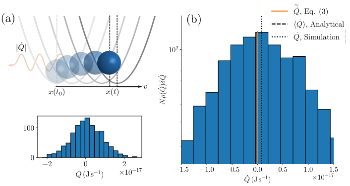
Figure 1: (a) A Brownian particle dissipates energy as heat when pulled by a harmonic trap. Initially, $t=t_{0}$ and the particle is at the trap center $x(t_{0})$. Translating the trap through space forces the average particle position to be higher on the potential. During the process, heat is dissipated at a rate $|\dot{Q}|$ into the environment. (b) Histogram of the heat dissipated to the environment from a simulation of the overdamped Langevin dynamics over 1000 noise realizations (SM Sec. 2). Heat rate from Eq. (3) (orange) agrees with the sample mean from the simulations (black line hidden by orange line) and the analytical mean (black dotted line).

Generally, observables like the heat rate can be difficult to predict a priori without a physical model. However, predictions of the heat rate and the other nonequilibrium observables satisfying Eq. (1) are possible through the speed limit. For the heat rate $\widetilde{\dot{Q}}$, we express the true rate from Eq. (1) as $|\dot{Q}|=\tau_{Q}^{-1}\Delta\epsilon$. Truncating Eq. (2) to first order, we can estimate $\widetilde{\tau}_{Q}^{-1}\Delta\hat{\epsilon}\approx\tilde{\tau}^{-1}\Delta\hat{\epsilon}$ . For the pulled particle, the predicted heat rate

$$|\widetilde{\dot{Q}}|=\tilde{\tau}_{Q}^{-1}\Delta\hat{\epsilon}\approx|v|\Delta\hat{\epsilon}/\Delta\hat{x},$$ (3)

is entirely in terms of known quantities from the experimental setup: the pulling speed and the uncertainties in the particle position and energy (SM Sec. 2). Take a particle with radius $1\mu$m in a trap with a force constant $k_{f}=6.67\times 10^{-7}$ N m^-1 being pulled at a speed [61] $|v|=1$ $\mu$m s^-1 through water, which has a viscosity $\eta=10^{-3}$ Pa s at 296.5 K . Under these conditions, the standard deviation in position is known to be $\Delta\hat{x}\approx\sigma_{\hat{x}}=\sqrt{k_{B}T/k_{f}}=78.32$ nm (errors can be of order $\pm 2$ nm [61]), and the standard deviation in energy is $\Delta\hat{\epsilon}\approx k_{B}T$. Using only these experimental values, Eq. (3) predicts a heat rate of $|\widetilde{\dot{Q}}|=|v|\sqrt{k_{f}/\beta}=5.22\times 10^{-20}$ W, which agrees well with the values from the Brownian dynamics model $|\langle\dot{Q}\rangle|=v^{2}/\gamma=1.885\times 10^{-20}$ W and our numerical simulations $6.69\times 10^{-19}$ W (SM Sec. 2).

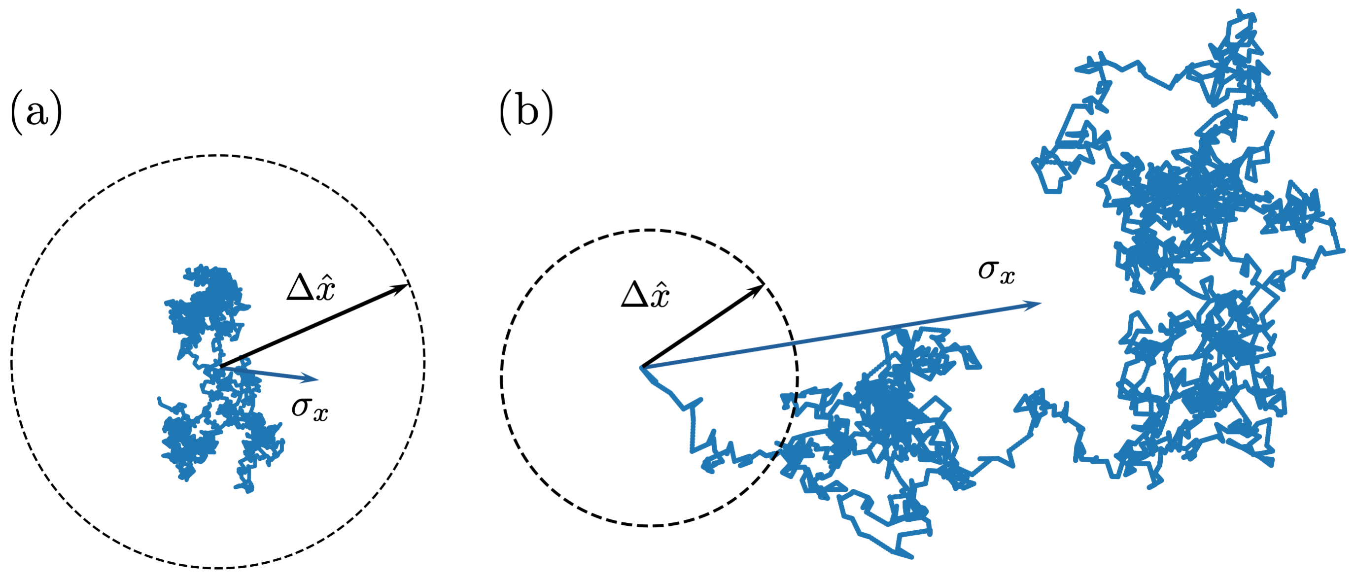
Figure 2: Illustration of conditions on the speed limit set by the Fisher information from the spatial resolution of experimental measurements of a particle undergoing Brownian motion. (a) A lower resolution (higher uncertainty) than required to measure position fluctuations of a Brownian particle leads to an upper bound on the speed limit, $\tilde{\tau}^{-1}\leq\tau^{-1}$. (b) A higher resolution (lower uncertainty) than required to measure position fluctuations leads to a lower bound, $\tilde{\tau}^{-1}\geq\tau^{-1}$.

Thermodynamic speed limits from experimental uncertainty.– As this example highlights, there are several advantages to predicting dissipation rates with the speed limit in Eq. (1). First, a single speed – the square root of the Fisher information – bounds multiple dissipation rates. Second, the Fisher information can transform into the variance of more accessible quantities (e.g., position, concentration). Third, while we used the true dynamics of the Brownian particle for validation, the coordinate transformation of the Fisher information, together with a linear model relating $\hat{r}$ and $\hat{x}$, bypasses the need for the full probability distribution of a dynamical model. These features are part of a more framework based on error propagation and the coordinate transformation of the Fisher information.

Take $X$ to be a quantity that is measurable by experiment. Because of the statistical error introduced by the measurement, we can model this quantity as a random variable with mean $\mu_{X}$, variance $\sigma_{X}^{2}$, and known distribution $\rho_{X}(x)$. But, imagine the system evolves under a dynamics described by the random variable $Y$ that is a known function $Y=f(X)$ of the state space $X$. From this perspective, standard propagation of error is a simple approximation of the distribution $\rho_{Y}(y)$ of $Y$ with only the first two moments, $\mu_{Y}$ and $\sigma_{Y}^{2}$: Gauss’s error propagation law [59] predicts the variance $\sigma_{Y}^{2}=\sigma_{X}^{2}(\partial_{X}f|_{X=\mu_{X}})^{2}$ and the Taylor expansion $Y=f(\mu_{X})+\partial_{X}f|_{X=\mu_{X}}(X-\mu_{X})$ predicts the mean $\mu_{Y}=f(\mu_{X})$.

Since the only quantities in the speed limit are variances and covariances, we can use Gauss’s law or its generalization to transform the speed limit. More generally, Taylor expanding a $m$ functions $f$ of $n$ measured quantities $\bm{X}$ gives

$$f_{i}(\bm{X})=f_{i}(\bm{\mu})+\gradient f_{i}^{\top}|_{\bm{X}=\bm{\mu}}(\bm{X}-\bm{\mu})+\varepsilon$$

with the Jacobian $\gradient f_{i}=(\partial_{X_{1}}f_{i},\partial_{X_{2}}f_{i},\ldots)^{\top}$. Taking the error to be uncorrelated with the inputs $X_{i}$, the covariances $(\bm{C}_{Y})_{kl}=\operatorname{cov}\left(f_{k},f_{l}\right)$ propagate from measured variables $(\bm{C}_{X})_{ij}=\operatorname{cov}\left(X_{i},X_{j}\right)$ [63]:

$$\bm{C}_{Y}=\gradient\bm{f}^{\top}\bm{C}_{X}\gradient\bm{f}+\sigma^{2}_{\varepsilon}.$$ (4)

Gauss’s law is a special case in which the function $f$ is linear, making the error $\varepsilon=0$ and $\sigma^{2}_{\varepsilon}=0$. From Eq. (4), even if these measurable variables are correlated with covariance matrix $\bm{C}$, one can predict the variance of several $\bm{f}(\bm{X})$ or a single function $Y=f(\bm{X})$.

The Brownian dynamics of a dragged colloidal particle are an example of the more general case in which $Y=\hat{r}$ is exactly a linear function of $X$. If the dependence is nonlinear (e.g., when $p_{Y}(y)$ is non-Gaussian), higher order terms may be neglected a desired level of approximation. Linear functions $\hat{r}=a+\bm{b}^{\top}\bm{X}$ have a distinct advantage here, even if the relation is nonlinear. (i) Linear statistical models saturate the bound $\tilde{\tau}_{Q}^{-1}=\tilde{\tau}^{-1}$ [24]. (ii) As was shown in Ref. [24], the optimal slope is $b_{\textrm{opt}}=\operatorname{cov}(X,\hat{r})/\Delta X^{2}=\dot{\mathcal{X}}/\Delta X^{2}$. Leveraging this result, we can choose a linear model and use $\dot{\mathcal{X}}/\Delta X^{2}$, which, as we have seen, avoids the need for the analytical expression for the nonequilibrium probability distribution over time when the rate $\dot{\mathcal{X}}$ and the variance $\Delta X^{2}$ are measurable.

The Fisher information in the speed limit obeys a coordinate transformation of the same form as Eq. (4). When $Y=\hat{r}$, the Fisher information transforms from the coordinates of a parameter space to the coordinates of a function space for a set of measurable quantities $\{X_{i}\}$:

$$\tilde{\tau}^{-2}=\Delta\hat{r}^{2}=\gradient f^{\top}(\bm{X})\,\bm{C}_{\bm{X}}\,\gradient f(\bm{X}).$$ (5)

This equation is an example of a coordinate transformation of the Fisher information, $I_{F}(\theta)=(\partial_{\theta}f(\theta))^{2}I_{F}(f(\theta))$ for a parameter, $I_{F}(\theta)$, to a function of that parameter, $I_{F}(f(\theta))$, in which $I_{F}(f(\theta))=\Delta\theta^{2}$. It is the multivariable version of $\tilde{\tau}^{-2}=(\partial_{\hat{x}}f)\Delta\hat{x}^{2}(\partial_{\hat{x}}f)$ used in the Brownian particle example; we recover Eq. (3) by recognizing that the Jacobian from $\theta=\hat{x}$ to $f(\theta)=\hat{r}$ is $|\partial_{\hat{x}}\hat{r}|=|d_{t}{\hat{x}}|/\Delta\hat{x}^{2}=|v|/\Delta\hat{x}^{2}$. The observables we consider here are expressible as a covariance with the rate $\hat{r}$, and the input variables, which have a finite variance, represent the state of the system. All together, these features of this this speed limit generally allow one to choose the input variances in $\bm{C}_{X}$ based on experimental convenience.

Necessary condition for upper bound.– For an observable $X$, only when $\tau_{X}^{-1}\leq\tau^{-1}\leq\tilde{\tau}^{-1}$ does the transformed speed limit $\tilde{\tau}^{-1}$ upper bound the heat rate, entropy production rate, and dissipated work. Whether this condition is satisfied depends on the relative magnitudes of experimental $\Delta\hat{x}$ and intrinsic fluctuations $\sigma_{x}$, which in our first example are due to Brownian motion $\sigma_{\hat{x}}$. For the harmonically trapped particle, the position is Gaussian distributed and the ratio of the true and error propagated speed limits is

$$\frac{\tau^{-1}}{\tilde{\tau}^{-1}}=\frac{\tau^{-1}}{\tilde{\tau}_{Q}^{-1}}=\frac{\sigma_{\hat{x}}}{\Delta\hat{x}}.$$ (6)

From this equality, whether the transformed speed limit is above or below depends on the measurement error, which can be assessed independently through experimental calibration. When the measurement error causes overestimates (underestimates) the intrinsic fluctuations such that $\Delta\hat{x}>\sigma_{\hat{x}}$, the speed limit will be overestimated $\tau^{-1}<\tilde{\tau}^{-1}$ (resp. underestimated), Fig. 2. The predicted speed limit is exact when there is no measurement error $\mathcal{E}$. Eq. (6) holds for systems with a linear or quadratic relation between $\hat{r}$ and the experimentally accessible variable $\hat{x}$.

From Eq. (6), it also follows that the measurement error also determines whether predictions of $|\widetilde{\dot{Q}}|$ are above or below the true heat rate $|\dot{Q}|$. For the pulled particle, the ratio of the Fisher informations clearly satisfies Eq. (6): The true Fisher information for the dragged particle is $I_{F}=\tau^{-2}=v^{2}\sigma_{\hat{x}}^{2}$ and the Fisher information propagated from the error in $\hat{x}$ is $\tilde{I}_{F}=v^{2}\Delta\hat{x}^{2}$ (SM Sec. 2). Numerically, when the error is $-|\mathcal{E}|=-10$ nm, the predicted heat rate $|\widetilde{\dot{Q}}|=6.67\times 10^{-21}$ W is less than the true mean value $|\dot{Q}|=1.88\times 10^{-20}$ W. For driven systems without experimental estimates of dissipation, we can predict the heat rate using the above equality. We confirmed this relation with several systems, including an active gel.

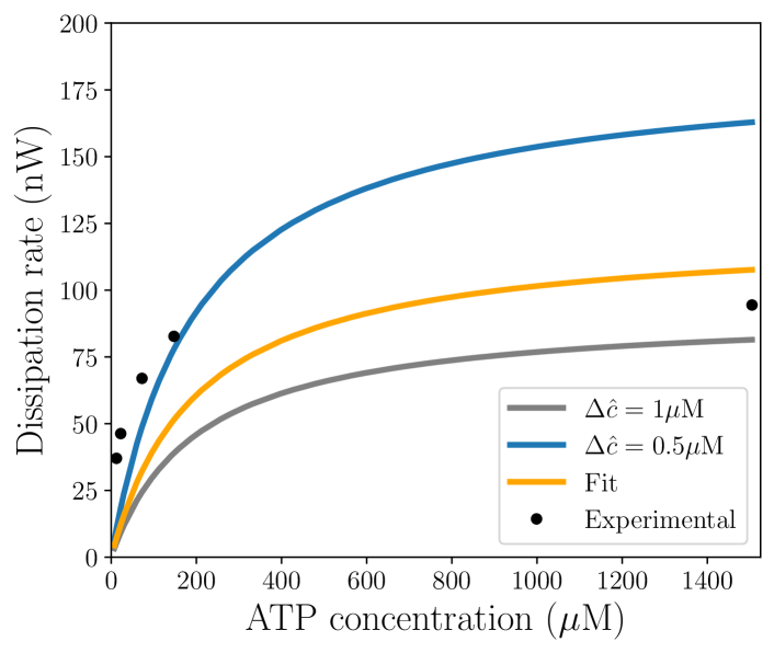
Figure 3: Comparison of predicted heat rate with experimental measurement. Dissipation rate versus ATP concentration with $[\text{K401}]=210$ nM, $[\text{MT}]=16$ $\mu$M. We use $\Delta\hat{\epsilon}=10^{-8}$ W $\times 1000$ s $=10^{-5}$ J and the rate constants: $k_{\text{D,ATP}}=96.4$ $\mu$M, $k_{\text{D,MT}}=17.4$ $\mu$M, and $k_{\text{cat}}=44s^{-1}$. The fit (orange) is the chemical kinetics model to the data (black points) from Ref. [11].

Prediction of energy dissipation rates for active gels.– With this framework and a necessary condition for upper bounding the true speed limit, we validated the predicted the heat rate against experimental measurements. This framework could be useful in guiding ongoing experiments on active materials, which continuously dissipate energy to sustain their nonequilibrium behavior. We analyzed microtuble active gels in which kinesin motors cross-link microtubule pairs and are driven by the chemical energy from ATP hydrolysis [11]. The first picocalorimetry measurements [12] suggest the energy efficiency of these materials is low: the minority of the input chemical energy propagating to productive emergent flows and the majority dissipated away as waste heat [11].

Given the advances required for these experiments [12] and their potential for designing the behavior of active materials [11], we compared our predictions to recent measurements of the energy dissipation rates. Using the concentration of chemical species in our framework, the predicted heat rate

$$|\widetilde{\dot{Q}}|=|\partial_{c}\hat{r}|\Delta\hat{c}\Delta\hat{\epsilon}=\frac{|d_{t}{\hat{c}}|}{\Delta\hat{c}}\Delta\hat{\epsilon}$$ (7)

is in terms of $|d_{t}{\hat{c}}|$ the average rate of the ATP hydrolysis reaction and the standard deviations in concentration and energy. The rate of ATP hydrolysis depends on the initial concentrations of kinesin, microtubule, ATP, and rate constants (SM Sec. 5). It can be determined with a previously parametrized model or without a model from the numerical derivative of concentration measurements.

The predicted heat rate agrees well with picocalorimetry measurements [11]. Figure 3 shows the predicted heat dissipation rate as a function of ATP concentration with all other concentrations fixed. The measured and predicted dissipation rates increase with the initial ATP concentration; the total sample volume is $0.5$ $\mu$L and the initial ATP concentration varies from $1.5-1500$ $\mu$M. Pipetting error is likely the dominant source of error in these measurements; propagating the 5% error in dose volume $\Delta\hat{c}=\hat{c}V^{-1}\Delta V$, the uncertainty in concentration is on the order of 1 $\mu$M for ATP concentrations in the range $12.5$-$190$ $\mu$M. Estimating the uncertainty in concentration $\Delta\hat{c}$ with 0.5 or 1 $\mu$M, the predicted heat rate is less than a factor of two of the experimental values. For low ATP concentrations, the prediction with $\Delta\hat{c}=0.5$ $\mu$M agrees better with the measured data than the fit with a chemical kinetics model (SM Eq. 19 [11]). Other potential sources of uncertainty are the pipetting protocol and fitted rate constants, which could also be accounted for in the prediction using Eq. (5). From a theoretical perspective, the heat rate in Eq. (7) only assumes a linear relationship between $r$ and $\hat{c}$ and does not require a known probability density function of the ATP concentration. We did confirm that the probability density for the number of ATP molecules over time in a Markov model (SM Sec. 6) satisfy the analog of Eq. (6).

Conclusions.– Fisher information is widely used in the statistical design of experiments: with known experimental errors, one can predict a priori the minimum error in a measured quantity [57]. Similarly, by leveraging its appearance in the thermodynamic speed limit here, we can, in principle, predict dissipation rates before performing an experiment. These predictions could be useful in determining the sensitivity of measurements to experimental control variables and in determining the experimental uncertainty needed for accurate measurements of dissipation rates. Used in these ways, the thermodynamic speed limit set by the Fisher information and the transformation to more convenient variables is a potentially efficient method to guide both the design of experiments and synthetic active materials. Since these speed limit predictions of dissipation rates are independent of specific dynamical evolution equation and the distance from thermal equilibrium, they apply across the length and time scales relevant for active materials.

I Acknowledgments