C-Mamba: Channel Correlation Enhanced State Space Models for Multivariate Time Series Forecasting

Abstract

In recent years, significant progress has been made in multivariate time series forecasting using Linear-based, Transformer-based, and Convolution-based models. However, these approaches face notable limitations: linear forecasters struggle with representation capacities, attention mechanisms suffer from quadratic complexity, and convolutional models have a restricted receptive field. These constraints impede their effectiveness in modeling complex time series, particularly those with numerous variables. Additionally, many models adopt the Channel-Independent (CI) strategy, treating multivariate time series as uncorrelated univariate series while ignoring their correlations. For models considering inter-channel relationships, whether through the self-attention mechanism, linear combination, or convolution, they all incur high computational costs and focus solely on weighted summation relationships, neglecting potential proportional relationships between channels. In this work, we address these issues by leveraging the newly introduced state space model and propose C-Mamba, a novel approach that captures cross-channel dependencies while maintaining linear complexity without losing the global receptive field. Our model consists of two key components: (i) channel mixup, where two channels are mixed to enhance the training sets; (ii) channel attention enhanced patch-wise Mamba encoder that leverages the ability of the state space models to capture cross-time dependencies and models correlations between channels by mining their weight relationships. Our model achieves state-of-the-art performance on seven real-world time series datasets. Moreover, the proposed mixup and attention strategy exhibits strong generalizability across other frameworks.

1 Introduction

Multivariate time series forecasting (MTSF) is essential in various fields, such as weather prediction [1], traffic management [2, 3, 4], economics [5], and event prediction [6]. MTSF aims to predict future values of temporal variations based on historical observations. Due to its great practical significance, numerous deep learning models have emerged in recent years, among which, Linear-based [7, 8, 9, 10], Transformer-based [11, 12, 13, 14, 15], and Convolution-based [16, 17, 18, 19] models develop rapidly and achieve notable performance.

Despite significant progress, existing models still have some shortcomings. Linear-based models are limited by their weak representation capabilities, while Convolution-based models are restricted by their small receptive fields. Consequently, both are ill-suited for long-term time series with a large number of variables. Transformer-based models, benefiting from their self-attention mechanism, possess global effective receptive fields, which allows them to better capture cross-time dependencies. However, this mechanism encodes each time step based on its attention to the entire sequence, resulting in quadratic complexity and redundant coding. Recently, the state space models [20, 21] (SSMs) have shown great potential in modeling long-term dependencies and have achieved progress in the computer vision field [22, 23]. SSMs adopt an RNN-like approach to capture long-range dependencies, achieving linear complexity and avoiding redundant coding.

In addition to cross-time dependencies, cross-channel dependencies are also vital for MTSF. As shown in Fig. 1, we depict the curves of two variables over time in the ETT dataset. We could draw the

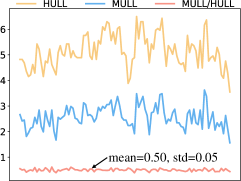
Figure 1: An illustration of the proportional relationship of variables in the ETT dataset. HULL means High UseLess Load and MULL means Middle UseLess Load.

following observations: (i) The two variables exhibit strong temporal characteristics similarity. (ii) They show a strong proportional relationship, that is, MULL (Middle UseLess Load) is roughly equivalent to half of HULL (High UseLess Load). These phenomena demonstrate the necessity of modeling cross-channel dependencies from proportional relationships. When dealing with cross-channel dependencies, there are generally two strategies: the Channel-Independent (CI) strategy that ignores cross-channel dependencies and the Channel-Dependent (CD) strategy that mixes channels according to a certain mechanism. Both strategies have their advantages and disadvantages. CD methods have higher capacity but lack robustness for distributionally drifted time series, whereas CI approaches trade capacity for robust predictions [24]. Many state-of-the-art models rely heavily on the CI strategy. These models [7, 14, 10] treat multivariate time series as independent univariate time series and simply treat different channels as different training samples. For others [18, 15, 19] considering cross-channel dependencies, whether through the self-attention mechanism, linear combination, or convolution, they all pay a large computational cost, and only regard the relationship between channels as a weighted summation relationship while ignoring their proportional relationship.

To better capture cross-time and cross-channel dependencies, we propose C-Mamba, a channel-enhanced state space model. First, to address the oversmoothing caused by the CD strategy, we introduce a channel mixup strategy, inspired by mixup data augmentation used in image classification [25, 26, 27] and time series data [28, 29]. This strategy fuses two channels via a linear combination for training. The generated virtual channels integrate characteristics from different channels while retaining their shared cross-time dependencies, which is expected to improve the generalizability of models. Then, a channel attention enhanced patch-wise Mamba encoder is introduced to capture both cross-time and cross-channel dependencies. For cross-time dependencies, we capture them with the selective state space mechanism, i.e., Mamba. While Mamba performs excellently in language sequences, for time series data, the lack of semantic information in a single time step limits its ability. Therefore, following the patching operation proposed by PatchTST [14], we introduce a patch-wise Mamba module, capturing temporal dependencies among various time patches. For cross-channel dependencies, we propose to model them via channel attention, a lightweight mechanism that considers various relationships between channels, including both weighted summation relationships and proportional relationships. Technically, our main contributions are summarized as follows:

• We dive into cross-channel dependencies in multivariate time series and propose a general framework, namely channel mixup and channel attention, capturing cross-channel dependencies while avoiding the oversmoothing problem caused by the CD strategy.

• We propose C-Mamba, a patch-wise state space model that captures cross-time dependencies through the selective state space mechanism and models cross-channel dependencies via channel mixup and channel attention.

• Experiments on seven real-world benchmarks demonstrate that our proposed framework achieves superior performance. We extensively apply the proposed channel mixup and channel attention to other models, indicating the broad versatility of our method.

2 Related Work

2.1 State Space Models

Traditional state space models (SSMs), such as hidden Markov models and recurrent neural networks (RNNs), process sequences by storing messages in their hidden states and using these states along with the current input to update the output. This recurrent mechanism limits their training efficiency and leads to problems like vanishing and exploding gradients [30]. Recently, several SSMs with linear-time complexity have been proposed, including S4 [31], H3 [32], and RWKV [33]. Mamba [21] further enhances S4 by introducing a data-dependent selection mechanism that balances short-term and long-term dependencies. Mamba has demonstrated powerful long-sequence modeling capabilities and has been successfully extended to the visual [22, 23] and graph domains [34].

2.2 Mixup

Mixup is an effective data augmentation technique widely used in vision [25, 26, 27], natural language processing [35, 36], and more recently, time series analysis [28, 29]. The vanilla mixup technique randomly mixes two input data samples via linear interpolation. Its variants extend this by mixing either input samples or hidden embedding to gain better generalization. In multivariate time series, each sample contains multiple time series. Hence, rather than mixing two samples, our proposed channel mixup mixes time series of the same sample. This strategy not only enhances the generalization of models but also facilitates the CD approach.

2.3 Attention Mechanism

The attention mechanism can be interpreted as a data-driven approach that assigns weights to each data point based on observations from the entire sequence. There are various types of attention mechanisms, such as self-attention [37], channel attention [38], and spatial attention [39], all of which play important roles in current models. In time series analysis, the self-attention mechanism has garnered particular interest [12, 14, 15]. While spatial attention is suited for data with spatial information, channel attention is applicable to any multivariate or multichannel data. Recent work [40] explores channel and frequency attention of time series in the frequency domain. However, we assume that the correlations between different channels remain stable over time. Thus, the vanilla channel attention could well capture these dependencies.

3 Preliminary

3.1 Multivariate Time Series Forecasting

In multivariate time series forecasting, given the historical time series $\mathbf{X}=\{\mathbf{x}_{1},...,\mathbf{x}_{L}\}\in\mathbb{R}^{L\times V}$ with a look-back window $L$ and the number of channels $V$, the goal is to predict the $T$ future values $\mathbf{Y}=\{\mathbf{x}_{L+1},...,\mathbf{x}_{L+T}\}\in\mathbb{R}^{T\times V}$. In the following sections, we denote $\textbf{X}_{t,:}$ as the value of all channels at time step $t$, and $\textbf{X}_{:,v}$ as the entire sequence of the channel indexed by $v$. The same annotation also applies to Y. In this paper, we focus on the long-term series forecasting task, where the prediction length is greater than or equal to 96.

3.2 Mamba

Given input $\mathbf{x}(t)\in\mathbb{R}$, the continuous state space mechanism produces a response $\mathbf{y}(t)\in\mathbb{R}$ based on the observation of hidden state $\mathbf{h}(t)\in\mathbb{R}^{N}$ and the input $\mathbf{x}(t)$, which can be formulated as:

$$\mathbf{h}^{\prime}(t) =\mathbf{A}\mathbf{h}(t)+\mathbf{B}\mathbf{x}(t),$$ (1)

$$\mathbf{y}(t) =\mathbf{C}\mathbf{h}(t),$$

where $\mathbf{A}\in\mathbb{R}^{N\times N}$ is the state transition matrix, $\mathbf{B}\in\mathbb{R}^{N\times 1}$ and $\mathbf{C}\in\mathbb{R}^{1\times N}$ are projection matrices. When the input and response contain $V$ channels, i.e., $\mathbf{x}(t)\in\mathbb{R}^{V}$ and $\mathbf{y}(t)\in\mathbb{R}^{V}$, the SSM is applied independently to each channel, that is, $\mathbf{A}\in\mathbb{R}^{V\times N\times N}$, $\mathbf{B}\in\mathbb{R}^{V\times N}$, and $\mathbf{C}\in\mathbb{R}^{V\times N}$. For efficient memory utilization, $\mathbf{A}$ can be compressed to $V\times N$. Hereafter, unless otherwise stated, we only consider multichannel systems and the compressed form of $\mathbf{A}$. For the discrete system, Eq. 1 could be discretized as:

$$\overline{\mathbf{A}} =\exp(\Delta\mathbf{A}),$$ (2)

$$\overline{\mathbf{B}} =(\Delta\mathbf{A})^{-1}(\exp(\Delta\mathbf{A})-\mathbf{I})\Delta\mathbf{B},$$

$$\mathbf{h}_{t} =\overline{\mathbf{A}}\mathbf{h}_{t-1}+\overline{\mathbf{B}}\mathbf{x}_{t},$$

$$\mathbf{y}_{t} =\mathbf{C}\mathbf{h}_{t},$$

where $\Delta\in\mathbb{R}^{V}$ is the sampling time interval. The above operation could be easily computed via a global convolution:

$$\overline{\mathbf{K}} =(\mathbf{C}\overline{\mathbf{B}},\mathbf{C}\overline{\mathbf{A}}\overline{\mathbf{B}},...,\mathbf{C}\overline{\mathbf{A}}^{L-1}\overline{\mathbf{B}}),$$ (3)

$$\mathbf{Y} =\mathbf{X}\ast\overline{\mathbf{K}},$$

where $L$ is the length of the sequence.

Selective scan mechanism Previous methods keep transfer parameters (e.g., $\mathbf{B}$ and $\mathbf{C}$) unchanged during sequence processing, ignoring their relationships with the input. Mamba adopts a selective scan strategy where $\mathbf{B}\in\mathbb{R}^{L\times V\times N}$, $\mathbf{C}\in\mathbb{R}^{L\times V\times N}$, and $\Delta\in\mathbb{R}^{L\times V}$ are derived from the input $\mathbf{X}\in\mathbb{R}^{L\times V}$. Such a data-dependent mechanism allows Mamba to perceive the contextual information of the input, enabling it to selectively perform state transitions.

4 Methodology

The overall structure of our C-Mamba is illustrated in Fig. 2. Before training, the channel mixup module mixes the input multivariate time series in the channel dimension. Then, we make use of the vanilla Mamba module followed by the channel attention module as our core architecture and propose our C-Mamba block, which exploits both cross-time and cross-channel dependencies. C-Mamba takes patch-wise sequences as input and makes predictions via a single linear layer. The details will be discussed in the following sections.

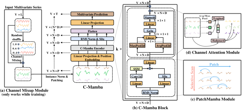
Figure 2: The overall framework of C-Mamba. (a) Channel mixup module, only working during training, fuses the channels of one sample and produces a new sample, which then serves as a virtual sample. New samples are normalized via instance norm and divided into different patches before being fed into the model. (b) C-Mamba block consists of two parts: the patch-wise Mamba module and channel attention before residual connection. (c) PatchMamba module is applied to capture cross-time dependencies. (d) Channel attention module captures cross-channel dependencies.

4.1 Channel Mixup

Previous mixup methods [25] mix two training samples via linear interpolation. For two feature-target vectors $(x_{i},y_{i})$ and $(x_{j},y_{j})$ randomly drawn from the training set, the process is defined as:

$$\tilde{x} =\lambda x_{i}+(1-\lambda)x_{j},$$ (4)

$$\tilde{y} =\lambda y_{i}+(1-\lambda)y_{j},$$

where $(\tilde{x},\tilde{y})$ is the synthesized virtual sample, and $\lambda\in[0,1]$. For multivariate time series, directly migrating the vanilla mixup often yields subpar results and may degrade model performance [28]. The reason might be that mixing samples drawn from different time intervals would disrupt the temporal characteristics of the dataset, such as periodicity, etc. However, different channels of multivariate time series share similar temporal characteristics, which is the reason why the CI strategy works [24]. Mixing different channels could introduce new variables while preserving their shared temporal features. Considering that the CD strategy tends to cause overfitting due to its lack of robustness to distributionally drifted time series [24], training with unseen channels should mitigate this issue. Generally, the channel mixup could be formulated as:

$$\textbf{X}^{\prime} =\textbf{X}_{:,i}+\lambda\textbf{X}_{:,j},~{}i,j=0,...,V-1,$$ (5)

$$\textbf{Y}^{\prime} =\textbf{Y}_{:,i}+\lambda\textbf{Y}_{:,j},~{}i,j=0,...,V-1,$$

where $\textbf{X}^{\prime}\in~{}\mathbb{R}^{L\times 1}$ and $\textbf{Y}^{\prime}\in~{}\mathbb{R}^{T\times 1}$ are hybrid channels resulting from the linear combination of channel $i$ and channel $j$. $\lambda\sim N(0,\sigma^{2})$ is the linear combination coefficient with $\sigma$ as the standard derivation. We use a normal distribution with a mean of $0$, ensuring that the overall characteristics of each channel remain unchanged. In practice, as shown in Alg. 1, we mix the channels of each sample and replace the original sample with the constructed virtual sample:

0:  training data $\mathbf{X}\in\mathbb{R}^{L\times V},\mathbf{Y}\in\mathbb{R}^{T\times V}$; standard derivation $\sigma$; the number of channels $V$

1:  perm = randperm($V$) # perm$\in\mathbb{R}^{V}$

2:  $\lambda$ = normal(mean=0, std=$\sigma$, size=($V$,))

3:  $\mathbf{X}^{\prime}$ = $\mathbf{X}$ + $\lambda$ * $\mathbf{X}$[:, perm]

4:  $\mathbf{Y}^{\prime}$ = $\mathbf{Y}$ + $\lambda$ * $\mathbf{Y}$[:, perm]

4:  $(\mathbf{X}^{\prime},\mathbf{Y}^{\prime})$

Algorithm 1 Channel mixup for multivariate time series forecasting

where $\text{randperm}(V)$ generates a randomly arranged array of $0\sim V-1$.

4.2 C-Mamba Block

Our proposed C-Mamba block consists of two key components: the patch-wise Mamba module and the channel attention module, which capture cross-time and cross-channel dependencies respectively.

4.2.1 PatchMamba

Mamba has demonstrated significant potential in NLP [21], CV [23, 22], and stock prediction [41]. In these fields, consistency in semantic information allows treating words, picture patches, or stock indicators as tokens. However, in multivariate time series, different channels may have completely different physical meanings [15], making it unsuitable to treat channels at the same time point as a token. While a single time step of each channel lacks semantic meaning, patching [42, 14] aggregates time points into subseries-level patches, enriching the semantic information and local receptive fields of tokens. Hence, we retain the structure of the vanilla Mamba module while dividing the input time series into patches to serve as the input of the Mamba module.

Patching Given multivariate time series $\mathbf{X}$, for each univariate series $\mathbf{X}_{:v}\in\mathbb{R}^{L}$, we divide it into patches via moving window with patch length $P$ and stride $S$:

$$\hat{\mathbf{X}}_{:v}=\text{Patching}(\mathbf{X}_{:v}),$$ (6)

where $\hat{\mathbf{X}}_{:v}\in\mathbb{R}^{N\times P}$ is a sequence of patches and $N=\lfloor\frac{(L-P)}{S}\rfloor+2$ is the number of patches.

4.2.2 Channel Attention

Fig. 2 (b) and (d) illustrate the structure of the channel attention module. For the patch-wise multivariate time series embedding after the $l^{th}$ PatchMamba module $\mathbf{H}_{l}\in\mathbb{R}^{V\times N\times D}$, the channel attention could be formulated as:

$$\mathbf{Att}_{l}=\text{sigmoid}(\text{MLP}(\text{MaxPool}(\mathbf{H}_{l}))+\text{MLP}(\text{AvgPool}(\mathbf{H}_{l}))),$$ (7)

which could be elaborated as:

$$\mathbf{Att}_{l}=\text{sigmoid}(\mathbf{W}_{1}(\text{Gelu}(\mathbf{W}_{0}\mathbf{F}_{max}^{l}))+\mathbf{W}_{1}(\text{Gelu}(\mathbf{W}_{0}\mathbf{F}_{avg}^{l}))).$$ (8)

Here, AvgPool and MaxPool are applied to the last two dimensions, generating descriptors $\mathbf{F}_{max}^{l}\in\mathbb{R}^{V\times 1\times 1}$ and $\mathbf{F}_{avg}^{l}\in\mathbb{R}^{V\times 1\times 1}$ that reflect the overall characteristics of each channel. MLP, parameterized by $\mathbf{W}_{0}\in\mathbb{R}^{V/r\times V}$ and $\mathbf{W}_{1}\in\mathbb{R}^{V\times V/r}$, is shared by both descriptors. $r$, controlling the parameter complexity, denotes the reduction ratio. It is essential for time series with hundreds of channels. We tune it in $\{2,4,8\}$. $\mathbf{Att}_{l}\in\mathbb{R}^{V\times 1\times 1}$ measures the weight of different channels based on their correlations. The output of the channel attention module is denoted as:

$$\mathbf{CA}_{l}=\mathbf{Att}_{l}\odot\mathbf{H}_{l}.$$ (9)

4.3 Overall Pipeline

Here, we summarize the previous description and outline the process of training and testing our model. In the training stage, given a sample $\{\mathbf{X},\mathbf{Y}\}$, it is converted to a virtual sample via channel mixup, followed by instance normalization that mitigates the distribution shifts:

$$\mathbf{X}^{\prime},\mathbf{Y}^{\prime} =\text{Mixup}(\mathbf{X},\mathbf{Y}),$$ (10)

$$\mathbf{X}^{\prime}_{norm} =\text{InstanceNorm}(\mathbf{X}^{\prime}).$$

Next, each channel is transformed into patches with the same patch length $P$ and patch number $N$. The patch-wise tokens are then linearly projected to vectors with size $D$ followed by a learnable position encoding $\mathbf{W}_{pos}$. The process could be formulated as:

$$\hat{\mathbf{X}} =\text{Patching}(\mathbf{X}^{\prime}_{norm}),$$ (11)

$$\mathbf{Z}_{0} =\hat{\mathbf{X}}\mathbf{W}_{p}+\mathbf{W}_{pos},$$

where $\hat{\mathbf{X}}\in\mathbb{R}^{V\times N\times P}$, $\mathbf{W}_{p}\in\mathbb{R}^{P\times D}$, $\mathbf{W}_{pos}\in\mathbb{R}^{N\times D}$, and $\mathbf{Z}_{0}\in\mathbb{R}^{V\times N\times D}$. $\mathbf{Z}_{0}$ is then fed into the C-Mamba encoder, consisting of $k$ C-Mamba blocks:

$$\mathbf{H}_{l} =\text{PatchMamba}(\mathbf{Z}_{l-1}),$$ (12)

$$\mathbf{Z}_{l} =\mathbf{Att}_{l}(\mathbf{H}_{l})\odot\mathbf{H}_{l}+\mathbf{Z}_{l-1},$$

where PatchMamba indicates the PatchMamba module and $l=1,...,k$. Our prediction is generated by a linear projection layer parameterized by $\mathbf{W}_{proj}\in\mathbf{R}^{(N*D)\times T}$:

$$\hat{\mathbf{Y}}_{p}=\text{Flatten}(\text{Silu}(\text{RMS}(\mathbf{Z}_{k})))\mathbf{W}_{proj},$$ (13)

where RMS denotes RMS norm and $\hat{\mathbf{Y}}_{p}\in\mathbb{R}^{V\times T}$.

In the testing stage, we remove the channel mixup module and only test on the original testing set.

5 Experiments

Dataset We evaluate our proposed C-Mamba on seven well-established datasets: ETTm1, ETTm2, ETTh1, ETTh2, Electricity, Weather, and Traffic. All of these datasets are publicly available [13]. We follow the public splits and apply zero-mean normalization to each dataset. More details about datasets are provided in Appendix 5.

Baselines We select ten advanced models as our baselines, including (i) Linear-based models: DLinear [7], RLinear [8], TiDE [9], TimeMixer [10]; (ii) Transformer-based models: Crossformer [12], PatchTST [14], iTransformer [15]; and (iii) Convolution-based models: MICN [17], TimesNet [18], ModernTCN [19].

Implementation We fix the look-back window $L=96$ and report the Mean Squared Error (MSE) as well as the Mean Absolute Error (MAE) for four prediction lengths $T\in\{96,192,336,720\}$. We reuse most of the baseline results from iTransformer [15] but we rerun MICN [17], TimeMixer [10], and ModernTCN [19] due to their different experimental settings. All experiments are repeated five times, and we report the mean. More details about hyperparameters can be found in Appendix A.2.

Table 1: Average results of the long-term forecasting task with prediction lengths $T\in\{96,192,336,720\}$. We fix the look-back window $L=96$ and report the average performance of all prediction lengths. The best is highlighted in red and the runner-up in blue. Full results are provided in Appendix D.1.

Models	C-Mamba  (Ours)		ModernTCN (2024)		iTransformer (2023c)		TimeMixer (2023)		RLinear (2023)		PatchTST (2022)		Crossformer (2022)		TiDE (2023)		TimesNet (2022)		MICN (2022)		DLinear (2023)
Metric	MSE	MAE	MSE	MAE	MSE	MAE	MSE	MAE	MSE	MAE	MSE	MAE	MSE	MAE	MSE	MAE	MSE	MAE	MSE	MAE	MSE	MAE
ETTm1	0.383	0.396	0.386	0.401	0.407	0.410	0.384	0.397	0.414	0.407	0.387	0.400	0.513	0.496	0.419	0.419	0.400	0.406	0.407	0.432	0.403	0.407
ETTm2	0.279	0.327	0.278	0.322	0.288	0.332	0.279	0.325	0.286	0.327	0.281	0.326	0.757	0.610	0.358	0.404	0.291	0.333	0.339	0.386	0.350	0.401
ETTh1	0.432	0.432	0.445	0.432	0.454	0.447	0.470	0.451	0.446	0.434	0.469	0.454	0.529	0.522	0.541	0.507	0.485	0.450	0.559	0.524	0.456	0.452
ETTh2	0.373	0.398	0.381	0.404	0.383	0.407	0.389	0.409	0.374	0.398	0.387	0.407	0.942	0.684	0.611	0.550	0.414	0.427	0.580	0.526	0.559	0.515
Electricity	0.176	0.266	0.197	0.282	0.178	0.270	0.183	0.272	0.219	0.298	0.216	0.304	0.244	0.334	0.251	0.344	0.192	0.295	0.185	0.296	0.212	0.300
Weather	0.244	0.271	0.240	0.271	0.258	0.279	0.245	0.274	0.272	0.291	0.259	0.281	0.259	0.315	0.271	0.320	0.259	0.287	0.267	0.318	0.265	0.317
Traffic	0.446	0.283	0.546	0.348	0.428	0.282	0.496	0.298	0.626	0.378	0.555	0.362	0.550	0.304	0.760	0.473	0.620	0.336	0.544	0.319	0.625	0.383

5.1 Main Results

Overall performance The comprehensive results for multivariate long-term forecasting are presented in Table 1. We report the average performance for four prediction lengths $T\in\{96,192,336,720\}$ in the main text, with full results available in Appendix D.1. Compared to state-of-the-art methods, C-Mamba ranks top 1 in 9 out of the 14 settings of varying metrics and top 2 in 13 settings. Actually, across all prediction lengths and metrics, encompassing 70 settings, C-Mamba ranks top 1 in 40 settings and top 2 in 62 settings (detailed in Appendix D.1). Notably, for datasets with numerous time series, such as Electricity, Weather, and Traffic, C-Mamba performs as well as or better than iTransformer. iTransformer captures cross-channel dependencies via the self-attention mechanism, incurring high computational costs and focusing only on the weighted summation relationships. These results underscore the importance of proportional correlations and demonstrate our method’s effectiveness. For experiments with a longer look-back length, we provide the results in Appendix C.1.

Generalizability We evaluate the effectiveness of channel mixup and channel attention on four recent models: iTransformer [15] and PatchTST [14] (Transformer-based), RLinear [8] (Linear-based), and TimesNet [18] (Convolution-based). Among them, iTransformer and TimesNet adopt a CD strategy, while PatchTST and RLinear utilize a CI approach. We retain the original architectures of these models but process the input via channel mixup during training and insert the channel attention module into the original models. The modified frameworks are detailed in Appendix B.2. As shown in Table 2, our pipeline consistently improves performance over various models. For TimesNet and iTransformer, which have already taken cross-channel dependencies into account, the proposed modules do not result in major improvements. However, for PatchTST, which adopts a CI strategy, the proposed modules prevent oversmoothing and yield significant performance gains. Although RLinear also utilizes a CI strategy, its single linear layer limits the benefits of channel mixup and channel attention.

Table 2: Performance promotion obtained by our proposed channel mixup and channel attention when applying them to other frameworks. We fix the look-back window $L=96$ and prediction length $T=96$.

Method		iTransformer		PatchTST		RLinear		TimesNet
Metric		MSE	MAE	MSE	MAE	MSE	MAE	MSE	MAE
Electricity	Original	0.148	0.240	0.195	0.285	0.201	0.281	0.168	0.272
	w/ channel mixup and attention	0.142	0.238	0.159	0.254	0.195	0.276	0.161	0.267
	Promotion	4.1%	0.8%	18.5%	10.9%	3.0%	1.9%	4.2%	1.8%
Weather	Original	0.174	0.214	0.177	0.218	0.192	0.232	0.172	0.220
	w/ channel mixup and attention	0.165	0.207	0.165	0.207	0.187	0.231	0.170	0.217
	Promotion	5.2%	3.3%	6.8%	5.0%	2.6%	0.4%	1.2%	1.4%

5.2 Ablation Studies

Ablation of module design To validate the effectiveness of each module in C-Mamba, we conduct ablation studies on the channel mixup and channel attention modules. As seen in Table 3, we report the average performance across four prediction lengths while including full results in Appendix D.2. Overall, the joint use of both modules achieves state-of-the-art performance. In most cases, both modules could work independently and provide significant improvements. However, for the Traffic dataset, channel attention alone degrades the performance, confirming our assertion that the Channel-Dependent (CD) strategy without channel mixup suffers from distribution shifts and overfitting. A more detailed analysis of the effectiveness of channel mixup is presented in Section 5.3.

Table 3: Ablation of channel mixup and channel attention. We list the average MSE/MAE of different prediction lengths. Full results are provide in Appendix D.2.

Channel Mixup	Channel Attention	ETTm1		ETTm2		ETTh1		ETTh2		Electricity		Weather		Traffic
		MSE	MAE	MSE	MAE	MSE	MAE	MSE	MAE	MSE	MAE	MSE	MAE	MSE	MAE
-	-	0.391	0.405	0.286	0.333	0.436	0.437	0.376	0.402	0.191	0.277	0.258	0.280	0.449	0.283
✓	-	0.389	0.401	0.283	0.329	0.433	0.434	0.374	0.399	0.189	0.273	0.258	0.278	0.448	0.281
-	✓	0.388	0.401	0.284	0.331	0.442	0.436	0.377	0.400	0.186	0.277	0.245	0.274	0.529	0.310
✓	✓	0.383	0.396	0.279	0.327	0.432	0.432	0.373	0.398	0.176	0.266	0.244	0.271	0.446	0.283

Ablation of Mamba In this paper, we choose Mamba as our backbone rather than Transformers. Table 4 compares the patch-wise Transformer (PatchTST) [14] and our patch-wise Mamba (PatchMamba). PatchMamba is the vanilla Mamba with patch-wise time series input and the Channel-Independent (CI) strategy. Overall, PatchMamba outperforms PatchTST in 5 out of 7 datasets, especially those with numerous channels, such as Electricity and Traffic. Fig. 3 (a) and (b) illustrate the final embedding of different patches in ETTh2, showing that attention-based encoding (PatchTST) is more segmented, while SSM-based encoding (PatchMamba) is more discretized. In addition, different patches encoded by PatchTST exhibit a higher silhouette coefficient (SC) than those of PatchMamba, indicating greater similarity and redundancy between patch encoding in PatchTST, which may explain why PatchMamba outperforms PatchTST. Beyond prediction accuracy, we also compare their model complexity, including parameters and FLOPs. As shown in Fig. 3 (c) and (d), to achieve comparable performance, PatchTST requires a larger number of parameters and FLOPs, indicating the lightweight and efficient nature of Mamba.

Table 4: Mamba vs. Transformers.

Model	ETTm1		ETTm2		ETTh1		ETTh2		Electricity		Weather		Traffic
	MSE	MAE	MSE	MAE	MSE	MAE	MSE	MAE	MSE	MAE	MSE	MAE	MSE	MAE
PatchMamba	0.391	0.405	0.286	0.333	0.436	0.437	0.376	0.402	0.191	0.277	0.258	0.280	0.449	0.283
PatchTST	0.387	0.400	0.281	0.326	0.469	0.454	0.387	0.407	0.216	0.304	0.259	0.281	0.555	0.362

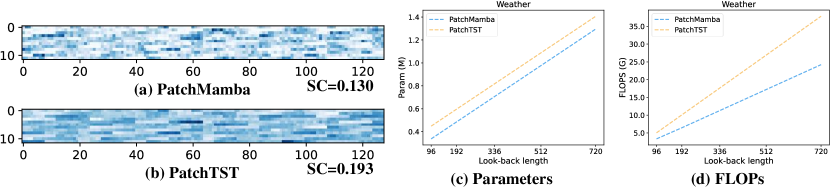
Figure 3: Comparisons of PatchMamba and PatchTST. (a) & (b) Visualization of patch embedding of ETTh2. There are 12 patches and the dimension of patch embedding is 128. SC measures the distance between sample groups and a higher coefficient means more intra-group similarity. (c) & (d) Complexity of PatchMamba and PachTST with the increment of the look-back window. The results are recorded on the Weather dataset with a batch size of 64 and a prediction length of 96.

5.3 Model Analysis

Effectiveness of channel mixup In Table 3, applying channel attention significantly degrades the performance on the Traffic dataset which contains 862 channels. However, as shown in Fig. 4 (a), the training loss of models with channel attention (yellow curve) is much lower than that without it (blue curve). While the training loss continues to decrease, the validation loss for models with channel attention increases, indicating serious oversmoothing caused by the CD strategy. The vanilla mixup (green curve) could alleviate this phenomenon to some extent, but it still fails to provide robust generalization. Thanks to channel mixup, our proposed C-Mamba (red curve) demonstrates stronger generalization capabilities and benefits from cross-channel dependencies.

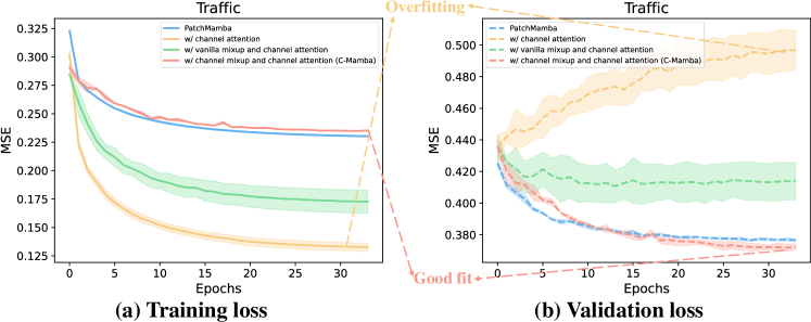
Figure 4: Loss curves for the Traffic dataset. PatchMamba is the vanilla model. The others are obtained by adding specified modules. (a) Training loss. (b) Validation loss.

Visualization of channel attention To validate whether the channel attention module successfully captures cross-channel dependencies, we visualize the generated attention of channels in each C-Mamba block. As shown in Fig. 5 (a), the channel attention module assigns weights to each channel based on its observations of all channels. Fig. 5 (b) and (d) show that channels with similar trends and values tend to have consistent attention weights. For channels with fewer similarities, models do assign them different attention, e.g., Fig. 5 (c). Notably, channels with negative correlations, as depicted in Fig. 5 (e), exhibit similar attention weights across different layers. The reason might be that channels with linear proportional relationships have proportional historical values. To ensure that the predicted values also remain proportional, their attention weights should be consistent. This confirms that channel attention could effectively identify proportional relationships between channels.

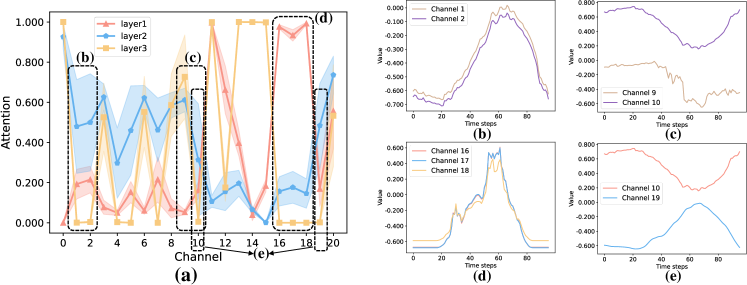
Figure 5: Visualization of the Weather dataset. (a) Channel attention across layers. (b) Series of channel 1 and 2. (c) Series of channel 9 and 10. (d) Series of channel 16, 17, and 18. (e) Series of channel 10 and 19.

6 Conclusions

We propose C-Mamba, a novel state space model for multivariate time series forecasting. To balance cross-time and cross-channel dependencies, C-Mamba consists of two key components: a channel mixup training strategy that enhances generalization and facilitates the CD approach, and a channel attention enhanced patch-wise Mamba encoder that captures cross-time dependencies via the selective state space mechanism and captures cross-channel dependencies using channel attention. Extensive experiments demonstrate that C-Mamba achieves state-of-the-art performance on seven real-world datasets. Notably, the channel mixup and channel attention modules could be seamlessly inserted into other models with minimal cost, showcasing remarkable framework versatility. In the future, we aim to explore more effective techniques to capture cross-time and cross-channel dependencies.

Appendix A Implementation Details

A.1 Dataset Descriptions

We conduct experiments on seven real-world datasets following the setups in previous works [Liu et al., 2023c, Nie et al., 2022]. (1) Four ETT (Electricity Transformer Temperature) datasets contain seven indicators from two different electric transformers in two years, each of which contains two different resolutions: 15 minutes (ETTm1 and ETTm2) and 1 hour (ETTh1 and ETTh2). (2) Electricity comprises the hourly electricity consumption of 321 customers in two years. (3) Weather contains 21 meteorological factors recorded every 10 minutes in Germany in 2020. (4) Traffic collects the hourly road occupancy rates from 862 different sensors on San Francisco freeways in two years. More details are provided in Table 5.

Table 5: Detailed dataset descriptions. $Channel$ indicates the number of variates. $Frequency$ denotes the sampling intervals of time steps. $Domain$ indicates the physical realm of each dataset. $Prediction~{}Length$ denotes the future time points to be predicted. The last row indicates the ratio of training, validation, and testing sets.

Dataset	Channel	Frequency	Domain	Prediction Length	Training:Validation:Testing
ETTm1	7	15 minutes	Electricity	$\{96,192,336,720\}$	6:2:2
ETTm2	7	15 minutes	Electricity	$\{96,192,336,720\}$	6:2:2
ETTh1	7	1 hour	Electricity	$\{96,192,336,720\}$	6:2:2
ETTh2	7	1 hour	Electricity	$\{96,192,336,720\}$	6:2:2
Electricity	321	1 hour	Electricity	$\{96,192,336,720\}$	7:1:2
Weather	21	10 minutes	Weather	$\{96,192,336,720\}$	7:1:2
Traffic	862	1 hour	Transportation	$\{96,192,336,720\}$	7:1:2

A.2 Hyperparameters

We conduct experiments on a single NVIDIA A30 24GB GPU. We utilize Adam [Kingma and Ba, 2014] optimizer with L2 loss and tune the initial learning rate in $\{0.0001,0.0005,0.001\}$. We fix the patch length at $16$ and the patch stride at $8$. The embedding of patches is selected from $\{128,256\}$. The number of C-Mamba blocks is searched in $\{2,3,4,5\}$. The reduction rate $r$ for channel attention is set from $\{2,4,8\}$. The standard deviation of channel mixup $\sigma$ is tuned from $0.5$ to $5$ with an adjustment step of $0.5$. The dropout rate is searched in $\{0,0.1\}$. For the PatchMamba module, we fix the dimension of the hidden state at $16$, the receptive field of convolution at $4$, and the expansion rate of the linear layer at $1$. To ensure robustness, we run our model five times under five random seeds in each setting. The average performance along with the standard deviation is presented in Table 6.

Table 6: Robustness of the proposed C-Mamba performance. The results are generated from five random seeds.

Dataset Horizon		ETTm1	ETTm2	ETTh1	ETTh2	Electricity	Weather	Traffic
96	MSE	0.324$\pm$0.005	0.175$\pm$0.001	0.374$\pm$0.002	0.290$\pm$0.002	0.147$\pm$0.001	0.157$\pm$0.001	0.414$\pm$0.002
	MAE	0.361$\pm$0.003	0.259$\pm$0.001	0.394$\pm$0.001	0.339$\pm$0.001	0.239$\pm$0.001	0.203$\pm$0.002	0.271$\pm$0.002
192	MSE	0.362$\pm$0.002	0.241$\pm$0.001	0.422$\pm$0.002	0.371$\pm$0.002	0.162$\pm$0.001	0.207$\pm$0.001	0.436$\pm$0.005
	MAE	0.382$\pm$0.001	0.304$\pm$0.001	0.423$\pm$0.001	0.390$\pm$0.000	0.253$\pm$0.001	0.250$\pm$0.001	0.277$\pm$0.002
336	MSE	0.395$\pm$0.002	0.302$\pm$0.001	0.462$\pm$0.006	0.415$\pm$0.003	0.178$\pm$0.001	0.266$\pm$0.001	0.445$\pm$0.002
	MAE	0.404$\pm$0.001	0.344$\pm$0.001	0.443$\pm$0.001	0.425$\pm$0.001	0.269$\pm$0.001	0.291$\pm$0.001	0.284$\pm$0.001
720	MSE	0.452$\pm$0.003	0.399$\pm$0.002	0.471$\pm$0.004	0.418$\pm$0.003	0.217$\pm$0.002	0.347$\pm$0.000	0.487$\pm$0.003
	MAE	0.438$\pm$0.001	0.399$\pm$0.002	0.469$\pm$0.003	0.437$\pm$0.003	0.303$\pm$0.002	0.342$\pm$0.001	0.299$\pm$0.002

Appendix B Baselines

B.1 Baseline Descriptions

We carefully selected 10 state-of-the-art models for our study. Their details are as follows:

1) DLinear [Zeng et al., 2023] is a Linear-based model utilizing decomposition and a Channel-Independent strategy. The source code is available at https://github.com/cure-lab/LTSF-Linear.

2) MICN [Wang et al., 2022] is a Convolution-based model featuring multi-scale hybrid decomposition and multi-scale convolution. The source code is available at https://github.com/wanghq21/MICN.

3) TimesNet [Wu et al., 2022] decomposes 1D time series into 2D time series based on multi-periodicity and captures intra-period and inter-period correlations via convolution. The source code is available at https://github.com/thuml/Time-Series-Library.

4) TiDE [Das et al., 2023] adopts a pure MLP structure and a Channel-Independent strategy. The source code is available at https://github.com/google-research/google-research/tree/master/tide.

5) Crossformer [Zhang and Yan, 2022] is a patch-wise Transformer-based model with two-stage attention that captures cross-time and cross-channel dependencies, respectively. The source code is available at https://github.com/Thinklab-SJTU/Crossformer.

6) PatchTST [Nie et al., 2022] is a patch-wise Transformer-based model that adopts a Channel-Independent strategy. The source code is available at https://github.com/yuqinie98/PatchTST.

7) RLinear [Li et al., 2023] is a Linear-based model with RevIN and a Channel-Independent strategy. The source code is available at https://github.com/plumprc/RTSF.

8) TimeMixer [Wang et al., 2023] is a fully MLP-based model that leverages multiscale time series. It makes predictions based on the multiscale seasonal and trend information of time series. The source code is available at https://github.com/kwuking/TimeMixer.

9) iTransformer [Liu et al., 2023c] is an inverted Transformer-based model that captures cross-channel dependencies via the self-attention mechanism and captures cross-time dependencies via linear projection. The source code is available at https://github.com/thuml/iTransformer.

10) ModernTCN [Luo and Wang, 2024] is a Convolution-based model with larger receptive fields. It utilizes depth-wise convolution to learn the patch-wise temporal information and two point-wise convolution layers to capture cross-time and cross-channel dependencies respectively. The source code is available at https://github.com/luodhhh/ModernTCN.

Notably, the source code of most of these models is available at https://github.com/thuml/Time-Series-Library.

B.2 Baseline Modification

In Section 5.1, we evaluate the effects of channel mixup and channel attention modules on four state-of-the-art models. During experiments, We retain the original architecture unchanged but process the input via channel mixup during training and insert the channel attention module into the original model. The modified frameworks of these models are shown in Fig. 6. All models adopt instance norm or RevIN [Kim et al., 2021] based on their original settings. We only tune the reduction rate $r$, standard deviation $\sigma$, and learning rate $lr$. The specific hyperparameters are listed in Table 7.

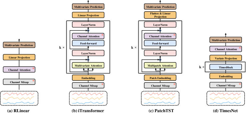
Figure 6: Modifications of the four chosen baselines. We retain the original architecture unchanged but apply channel mixup during training and insert the channel attention module into the original model. The ${\color[rgb]{1,0,0}*}$ modules represent channel mixup and channel attention.

Table 7: Hyperparameters for four models equipped with the channel mixup and channel attention module. $r$ denotes the reduction rate for channel attention. $\sigma$ indicates the standard derivation for channel mixup. $lr$ is the learning rate.

Dataset	Weather			Electricity
Hyperparameter	$r$	$\sigma$	$lr$	$r$	$\sigma$	$lr$
RLinear	2	0.5	0.005	4	1.0	0.001
iTransformer	2	0.5	0.0001	8	0.5	0.001
PatchTST	2	0.5	0.0001	4	1.0	0.001
TimesNet	2	0.1	0.001	8	0.5	0.001

Appendix C More Evaluation

C.1 Longer Look-back Length

Like other state-of-the-art models, our forecasting performance improves with larger historical windows, consistent with the assumption that a larger receptive field leads to better prediction performance. The results are illustrated in Fig. 7.

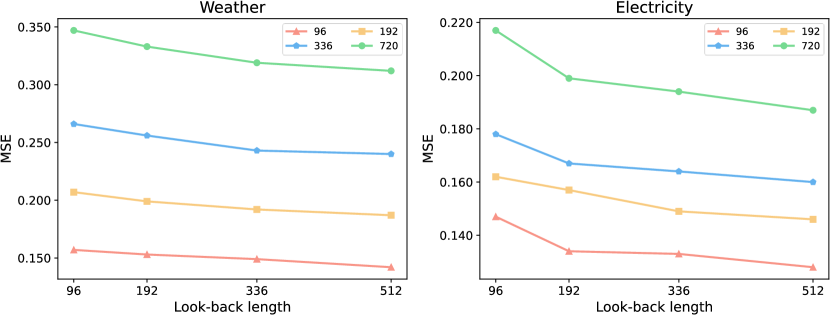
Figure 7: Performance promotion with longer look-back lengths.

Considering that the performance of different models is influenced by the look-back length, we further compare our model with state-of-the-art frameworks under the optimal look-back length. As shown in Table 8, we compare the performance of each model using their best look-back window. For C-Mamba, we search the look-back length in $\{96,192,336,512\}$ and ultimately select $512$ for both datasets. For other benchmarks, we rerun iTransformer since its look-back length is fixed at $96$ in the original paper, and we collect results for other models from tables in ModernTCN [Luo and Wang, 2024], TimeMixer [Wang et al., 2023], and TiDE [Das et al., 2023]. The results indicate that our model still achieves state-of-the-art performance.

Table 8: Full results of the long-term forecasting task under the optimal look-back window. We search the look-back window of C-Mamba in $\{96,192,336,512\}$ and finally choose $512$ for four prediction lengths. Avg means the average metrics for four prediction lengths. The best is highlighted in red and the runner-up in blue. We report the average results of five random seeds.

Models		C-Mamba  (Ours)		ModernTCN (2024)		iTransformer (2023c)		TimeMixer (2023)		RLinear (2023)		PatchTST (2022)		Crossformer (2022)		TiDE (2023)		TimesNet (2022)		MICN (2022)		DLinear (2023)
Metric		MSE	MAE	MSE	MAE	MSE	MAE	MSE	MAE	MSE	MAE	MSE	MAE	MSE	MAE	MSE	MAE	MSE	MAE	MSE	MAE	MSE	MAE
Electricity	96	0.128	0.221	0.129	0.226	0.132	0.228	0.129	0.224	0.140	0.235	0.129	0.222	0.219	0.314	0.132	0.229	0.168	0.272	0.159	0.267	0.153	0.237
	192	0.146	0.241	0.143	0.239	0.154	0.247	0.140	0.220	0.154	0.248	0.147	0.240	0.231	0.322	0.147	0.243	0.184	0.289	0.168	0.279	0.152	0.249
	336	0.160	0.256	0.161	0.259	0.172	0.266	0.161	0.255	0.171	0.264	0.163	0.259	0.246	0.337	0.161	0.261	0.198	0.300	0.196	0.308	0.169	0.267
	720	0.187	0.282	0.191	0.286	0.210	0.303	0.194	0.287	0.209	0.297	0.197	0.290	0.280	0.363	0.196	0.294	0.220	0.320	0.203	0.312	0.233	0.344
	Avg	0.155	0.250	0.156	0.253	0.167	0.261	0.156	0.246	0.169	0.261	0.159	0.253	0.244	0.334	0.159	0.257	0.192	0.295	0.182	0.292	0.177	0.274
Weather	96	0.142	0.191	0.149	0.200	0.162	0.212	0.147	0.197	0.175	0.225	0.149	0.198	0.153	0.217	0.166	0.222	0.172	0.220	0.161	0.226	0.152	0.237
	192	0.187	0.236	0.196	0.245	0.204	0.252	0.189	0.239	0.218	0.260	0.194	0.241	0.197	0.269	0.209	0.263	0.219	0.261	0.220	0.283	0.220	0.282
	336	0.240	0.273	0.238	0.277	0.256	0.290	0.241	0.280	0.265	0.294	0.245	0.282	0.252	0.311	0.254	0.301	0.280	0.306	0.275	0.328	0.265	0.319
	720	0.312	0.330	0.314	0.334	0.326	0.338	0.310	0.330	0.329	0.339	0.314	0.334	0.318	0.363	0.313	0.340	0.365	0.359	0.311	0.356	0.323	0.362
	Avg	0.220	0.257	0.224	0.264	0.237	0.273	0.222	0.262	0.247	0.279	0.226	0.264	0.230	0.290	0.236	0.282	0.259	0.287	0.242	0.298	0.240	0.300

C.2 Computational Cost

We report the computational cost introduced by the channel attention module in Table 9, quantified by FLOPs (G).

Table 9: Computational cost of channel attention. We use FLOPs (G) to measure the computational complexity.

Dataset	ETT	Weather	Electricity	Traffic
Channel	7	21	321	862
w/o channel attention	1.0762	3.2287	49.3529	66.2652
w/ channel attention	1.0783	3.2351	49.4674	66.4278
FLOPs increment	0.20%	0.20%	0.23%	0.25%

For a fair comparison, we conduct experiments on our C-Mamba with a fixed hidden size of $128$, three layers, and a batch size of 64 for the ETT, Weather, and Electricity datasets. Due to memory limitations, the batch size of the Traffic dataset is set to $32$. As shown in Table 9, the channel attention module has a negligible impact on the computational cost of models. Even for the Traffic dataset, which contains 862 channels, the increase in FLOPs is only 0.25%.

C.3 Hyperparameter Sensitivity

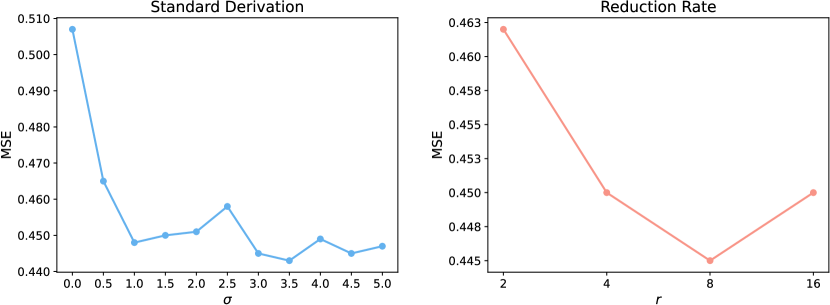
Figure 8: Hyperparameter sensitivity of the standard derivation $\sigma$ for channel mixup (left) and the reduction rate $r$ for channel attention (right).

We extensively evaluate the hyperparameters influencing the performance of C-Mamba. Specifically, we consider two factors: the standard derivation $\sigma$ for channel mixup and the reduction rate $r$ for channel attention. Experiments are conducted on the Traffic dataset with a fixed look-back window of $96$ and a prediction length of $336$. We adjust only the factors under consideration while keeping other hyperparameters consistent with Table 1. The results are shown in Fig. 8. As one of our core modules, $\sigma$ should be carefully selected to optimize the performance of channel mixup. Regarding channel attention, the reduction rate $r$ significantly influences both model complexity and performance. A well-chosen reduction rate can both reduce model complexity and enhance generalization ability. Therefore, the reduction rate is a hyperparameter that needs to be carefully tuned. Empirically, for datasets with a large number of channels ($\geq 200$), reducing the number of channels to around $100$ proves to be an effective choice.

C.4 Limitations

In this work, we mainly focus on the multivariate time series forecasting task with endogenous variables, meaning that the values we aim to predict and the values treated as features only differ in terms of time steps. However, real-world scenarios often involve the influence of exogenous variables on the variables we seek to predict, a topic extensively discussed in prior research [Wang et al., 2024b]. In addition, the experimental results show that our model exhibits significant improvements on some datasets with large-scale channels, such as Weather and Electricity. However, the improvements are relatively limited on the Traffic dataset, which contains 862 channels. This discrepancy could be attributed to the pronounced periodicity observed in traffic data compared to other domains. These periodic patterns are highly time-dependent, causing different channels to exhibit similar characteristics and obscuring their physical interconnections. Therefore, incorporating external variables and utilizing prior knowledge about the relationships between channels, such as the connectivity of traffic roads, might further enhance the prediction accuracy.

Appendix D Full Results

D.1 Full Main Results

Here, we present the complete results of all chosen models and our C-Mamba under four different prediction lengths in Table 10. Generally, the proposed C-Mamba demonstrates stable performance across various datasets and prediction lengths, consistently ranking among the top performers. Specifically, our model ranks top 1 in 40 out of 70 settings and ranks top 2 in 62 settings, while the runner-up, ModernTCN [Luo and Wang, 2024] ranks top 1 in only 20 settings and top 2 in 29 settings.

Table 10: Full results of the long-term forecasting task. We fix the look-back window $L=96$ and make predictions for $T=\{96,192,336,720\}$. Avg means the average metrics for four prediction lengths. The best is highlighted in red and the runner-up in blue. We report the average results of five random seeds.

Models		C-Mamba  (Ours)		ModernTCN (2024)		iTransformer (2023c)		TimeMixer (2023)		RLinear (2023)		PatchTST (2022)		Crossformer (2022)		TiDE (2023)		TimesNet (2022)		MICN (2022)		DLinear (2023)
Metric		MSE	MAE	MSE	MAE	MSE	MAE	MSE	MAE	MSE	MAE	MSE	MAE	MSE	MAE	MSE	MAE	MSE	MAE	MSE	MAE	MSE	MAE
ETTm1	96	0.324	0.361	0.317	0.362	0.334	0.368	0.320	0.355	0.355	0.376	0.329	0.367	0.404	0.426	0.364	0.387	0.338	0.375	0.317	0.367	0.345	0.372
	192	0.362	0.382	0.363	0.389	0.377	0.391	0.362	0.382	0.391	0.392	0.367	0.385	0.450	0.451	0.398	0.404	0.374	0.387	0.382	0.413	0.380	0.389
	336	0.395	0.404	0.403	0.412	0.426	0.420	0.396	0.406	0.424	0.415	0.399	0.410	0.532	0.515	0.428	0.425	0.410	0.411	0.417	0.443	0.413	0.413
	720	0.452	0.438	0.461	0.443	0.491	0.459	0.458	0.445	0.487	0.450	0.454	0.439	0.666	0.589	0.487	0.461	0.478	0.450	0.511	0.505	0.474	0.453
	Avg	0.383	0.396	0.386	0.401	0.407	0.410	0.384	0.397	0.414	0.407	0.387	0.400	0.513	0.496	0.419	0.419	0.400	0.406	0.407	0.432	0.403	0.407
ETTm2	96	0.175	0.259	0.173	0.255	0.180	0.264	0.176	0.259	0.182	0.265	0.175	0.259	0.287	0.366	0.207	0.305	0.187	0.267	0.182	0.278	0.193	0.292
	192	0.241	0.304	0.235	0.296	0.250	0.309	0.242	0.303	0.246	0.304	0.241	0.302	0.414	0.492	0.290	0.364	0.249	0.309	0.288	0.357	0.284	0.362
	336	0.302	0.344	0.308	0.344	0.311	0.348	0.303	0.339	0.307	0.342	0.305	0.343	0.597	0.542	0.377	0.422	0.321	0.351	0.370	0.413	0.369	0.427
	720	0.399	0.399	0.398	0.394	0.412	0.407	0.396	0.399	0.407	0.398	0.402	0.400	1.730	1.042	0.558	0.524	0.408	0.403	0.519	0.495	0.554	0.522
	Avg	0.279	0.327	0.278	0.322	0.288	0.332	0.279	0.325	0.286	0.327	0.281	0.326	0.757	0.610	0.358	0.404	0.291	0.333	0.339	0.386	0.350	0.401
ETTh1	96	0.374	0.394	0.386	0.394	0.386	0.405	0.384	0.400	0.386	0.395	0.414	0.419	0.423	0.448	0.479	0.464	0.384	0.402	0.417	0.436	0.386	0.400
	192	0.422	0.423	0.436	0.423	0.441	0.436	0.437	0.429	0.439	0.424	0.460	0.445	0.471	0.474	0.525	0.492	0.436	0.429	0.488	0.476	0.437	0.432
	336	0.462	0.443	0.479	0.445	0.487	0.458	0.472	0.446	0.479	0.446	0.501	0.466	0.570	0.546	0.565	0.515	0.491	0.469	0.599	0.549	0.481	0.459
	720	0.471	0.469	0.481	0.469	0.503	0.491	0.586	0.531	0.481	0.470	0.500	0.488	0.653	0.621	0.594	0.558	0.521	0.500	0.730	0.634	0.519	0.516
	Avg	0.432	0.432	0.445	0.432	0.454	0.447	0.470	0.451	0.446	0.434	0.469	0.454	0.529	0.522	0.541	0.507	0.485	0.450	0.559	0.524	0.456	0.452
ETTh2	96	0.290	0.339	0.292	0.340	0.297	0.349	0.297	0.348	0.288	0.338	0.302	0.348	0.745	0.584	0.400	0.440	0.340	0.374	0.355	0.402	0.333	0.387
	192	0.371	0.390	0.377	0.395	0.380	0.400	0.369	0.392	0.374	0.390	0.388	0.400	0.877	0.656	0.528	0.509	0.402	0.414	0.511	0.491	0.477	0.476
	336	0.415	0.425	0.424	0.434	0.428	0.432	0.427	0.435	0.415	0.426	0.426	0.433	1.043	0.732	0.643	0.571	0.452	0.452	0.618	0.551	0.594	0.541
	720	0.418	0.437	0.433	0.448	0.427	0.445	0.462	0.463	0.420	0.440	0.431	0.446	1.104	0.763	0.874	0.679	0.462	0.468	0.835	0.660	0.831	0.657
	Avg	0.373	0.398	0.381	0.404	0.383	0.407	0.389	0.409	0.374	0.398	0.387	0.407	0.942	0.684	0.611	0.550	0.414	0.427	0.580	0.526	0.559	0.515
Electricity	96	0.147	0.239	0.173	0.260	0.148	0.240	0.153	0.244	0.201	0.281	0.195	0.285	0.219	0.314	0.237	0.329	0.168	0.272	0.172	0.285	0.197	0.282
	192	0.162	0.253	0.181	0.267	0.162	0.253	0.168	0.259	0.201	0.283	0.199	0.289	0.231	0.322	0.236	0.330	0.184	0.289	0.177	0.287	0.196	0.285
	336	0.178	0.269	0.196	0.283	0.178	0.269	0.185	0.275	0.215	0.298	0.215	0.305	0.246	0.337	0.249	0.344	0.198	0.300	0.186	0.297	0.209	0.301
	720	0.217	0.303	0.238	0.316	0.225	0.319	0.227	0.312	0.257	0.331	0.256	0.337	0.280	0.363	0.284	0.373	0.220	0.320	0.204	0.314	0.245	0.333
	Avg	0.176	0.266	0.197	0.282	0.178	0.270	0.183	0.272	0.219	0.298	0.216	0.304	0.244	0.334	0.251	0.344	0.192	0.295	0.185	0.296	0.212	0.300
Weather	96	0.157	0.203	0.155	0.203	0.174	0.214	0.162	0.208	0.192	0.232	0.177	0.218	0.158	0.230	0.202	0.261	0.172	0.220	0.194	0.253	0.196	0.255
	192	0.207	0.250	0.202	0.247	0.221	0.254	0.208	0.252	0.240	0.271	0.225	0.259	0.206	0.277	0.242	0.298	0.219	0.261	0.240	0.301	0.237	0.296
	336	0.266	0.291	0.263	0.293	0.278	0.296	0.263	0.293	0.292	0.307	0.278	0.297	0.272	0.335	0.287	0.335	0.280	0.306	0.284	0.334	0.283	0.335
	720	0.347	0.342	0.341	0.343	0.358	0.349	0.345	0.345	0.364	0.353	0.354	0.348	0.398	0.418	0.351	0.386	0.365	0.359	0.351	0.387	0.345	0.381
	Avg	0.244	0.271	0.240	0.271	0.258	0.279	0.245	0.274	0.272	0.291	0.259	0.281	0.259	0.315	0.271	0.320	0.259	0.287	0.267	0.318	0.265	0.317
Traffic	96	0.414	0.271	0.550	0.355	0.395	0.268	0.473	0.287	0.649	0.389	0.544	0.359	0.522	0.290	0.805	0.493	0.593	0.321	0.521	0.310	0.650	0.396
	192	0.436	0.277	0.527	0.337	0.417	0.276	0.486	0.294	0.601	0.366	0.540	0.354	0.530	0.293	0.756	0.474	0.617	0.336	0.536	0.314	0.598	0.370
	336	0.445	0.284	0.537	0.342	0.433	0.283	0.488	0.298	0.609	0.369	0.551	0.358	0.558	0.305	0.762	0.477	0.629	0.336	0.550	0.321	0.605	0.373
	720	0.487	0.299	0.570	0.359	0.467	0.302	0.536	0.314	0.647	0.387	0.586	0.375	0.589	0.328	0.719	0.449	0.640	0.350	0.571	0.329	0.645	0.394
	Avg	0.446	0.283	0.546	0.348	0.428	0.282	0.496	0.298	0.626	0.378	0.555	0.362	0.550	0.304	0.760	0.473	0.620	0.336	0.544	0.319	0.625	0.383
$1^{\text{st}}$Count		17	23	9	11	7	6	4	3	2	3	0	0	0	0	0	0	0	0	2	0	0	0

D.2 Full Ablation Results

In the main text, we only present the improvements brought by the proposed modules in the average case. To validate the effectiveness of our design, we provide the complete results in Table 11 and Table 12. Consistent with our claims, channel attention alone can easily lead to oversmoothing. However, when combined with the channel mixup, our model consistently achieves state-of-the-art performance.

Table 11: Full results of ablation studies for ETTm1, ETTm2, ETTh1, and ETTh2. We fix the look-back window $L=96$ and make predictions for $T=\{96,192,336,720\}$. The best is highlighted in red and the runner-up in blue. We report the average results of five random seeds.

Channel Mixup	Channel Attention	Metric	ETTm1				ETTm2				ETTh1				ETTh2
			96	192	336	720	96	192	336	720	96	192	336	720	96	192	336	720
-	-	MSE	0.331	0.370	0.403	0.459	0.178	0.248	0.310	0.408	0.377	0.425	0.462	0.481	0.292	0.373	0.417	0.424
		MAE	0.372	0.389	0.411	0.450	0.264	0.309	0.350	0.408	0.398	0.428	0.445	0.476	0.342	0.393	0.430	0.443
✓	-	MSE	0.329	0.369	0.396	0.461	0.176	0.243	0.307	0.405	0.373	0.422	0.461	0.478	0.291	0.371	0.414	0.420
		MAE	0.364	0.386	0.407	0.444	0.260	0.305	0.347	0.403	0.394	0.423	0.445	0.475	0.340	0.390	0.425	0.439
-	✓	MSE	0.327	0.368	0.396	0.461	0.177	0.244	0.306	0.411	0.382	0.431	0.470	0.483	0.292	0.373	0.418	0.425
		MAE	0.363	0.387	0.407	0.447	0.262	0.307	0.347	0.409	0.399	0.427	0.445	0.474	0.341	0.391	0.428	0.442
✓	✓	MSE	0.324	0.362	0.395	0.452	0.175	0.241	0.302	0.399	0.374	0.422	0.462	0.471	0.290	0.371	0.415	0.418
		MAE	0.361	0.382	0.404	0.438	0.259	0.304	0.344	0.399	0.394	0.423	0.443	0.469	0.339	0.390	0.425	0.437

Table 12: Full results of ablation studies for Electricity, Weather, and Traffic. We fix the look-back window $L=96$ and make predictions for $T=\{96,192,336,720\}$. The best is highlighted in red and the runner-up in blue. We report the average results of five random seeds.

Channel Mixup	Channel Attention	Metric	Electricity				Weather				Traffic
			96	192	336	720	96	192	336	720	96	192	336	720
-	-	MSE	0.166	0.175	0.192	0.231	0.175	0.224	0.277	0.354	0.424	0.435	0.452	0.484
		MAE	0.253	0.263	0.279	0.312	0.216	0.259	0.297	0.347	0.272	0.276	0.284	0.301
✓	-	MSE	0.164	0.172	0.189	0.230	0.174	0.223	0.277	0.356	0.423	0.436	0.451	0.482
		MAE	0.250	0.259	0.275	0.310	0.214	0.256	0.295	0.346	0.270	0.274	0.281	0.298
-	✓	MSE	0.158	0.172	0.188	0.225	0.160	0.210	0.266	0.345	0.507	0.518	0.535	0.558
		MAE	0.253	0.265	0.280	0.311	0.206	0.252	0.293	0.344	0.313	0.303	0.309	0.314
✓	✓	MSE	0.147	0.162	0.178	0.217	0.157	0.207	0.266	0.347	0.414	0.436	0.445	0.487
		MAE	0.239	0.253	0.269	0.303	0.203	0.250	0.291	0.342	0.271	0.277	0.284	0.299

Appendix E Showcases

E.1 Comparison with Baselines

As depicted in Fig. 9, Fig. 10, Fig. 11, and Fig. 12, Fig. 13, Fig. 14, we visualize the forecasting results on the Electricity and Traffic dataset of our model, ModernTCN [Luo and Wang, 2024], and TimeMixer [Wang et al., 2023]. Overall, our model fits the data better. Especially when dealing with non-periodic changes. For instance, in Prediction-96 of the Electricity dataset, our model exhibits significantly better performance compared to the others.

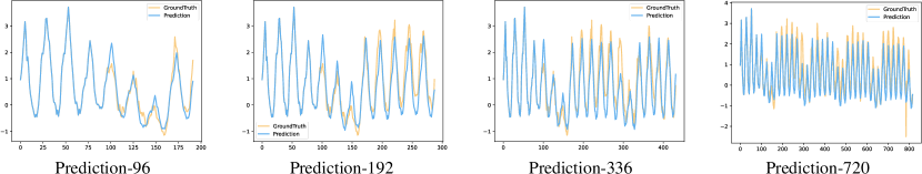
Figure 9: Prediction cases for Electricity under C-Mamba.

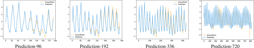
Figure 10: Prediction cases for Electricity under ModernTCN.

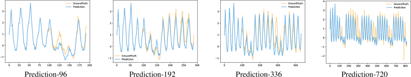
Figure 11: Prediction cases for Electricity under TimeMixer.

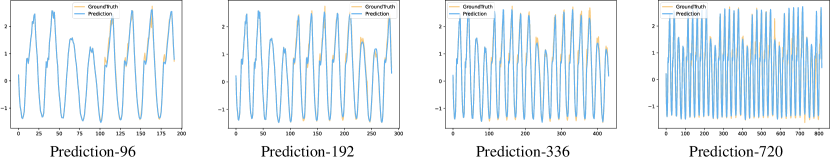
Figure 12: Prediction cases for Traffic under C-Mamba.

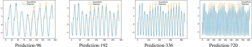
Figure 13: Prediction cases for Traffic under ModernTCN.

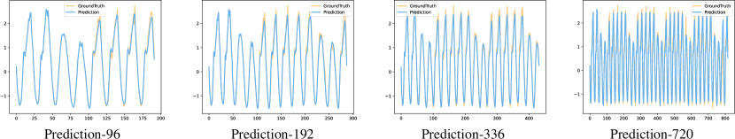
Figure 14: Prediction cases for Traffic under TimeMixer.

E.2 More Showcases

As shown in Fig. 15, Fig. 16, Fig. 17, Fig. 18, and Fig. 19, we visualize the forecasting results of other datasets under C-Mamba. The results demonstrate that C-Mamba achieves consistently stable performance under various datasets.

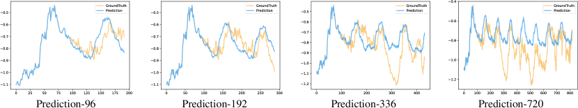
Figure 15: Prediction cases for ETTm1 under C-Mamba.

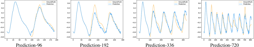
Figure 16: Prediction cases for ETTm2 under C-Mamba.

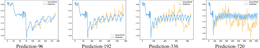
Figure 17: Prediction cases for ETTh1 under C-Mamba.

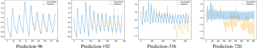
Figure 18: Prediction cases for ETTh2 under C-Mamba.

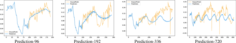
Figure 19: Prediction cases for Weather under C-Mamba.

References

- Chen et al. [2023] Shengchao Chen, Guodong Long, Tao Shen, Tianyi Zhou, and Jing Jiang. Spatial-temporal prompt learning for federated weather forecasting. arXiv preprint arXiv:2305.14244, 2023.
- Liu et al. [2023a] Zhanyu Liu, Chumeng Liang, Guanjie Zheng, and Hua Wei. Fdti: Fine-grained deep traffic inference with roadnet-enriched graph. In Joint European Conference on Machine Learning and Knowledge Discovery in Databases, pages 174–191. Springer, 2023a.
- Liu et al. [2023b] Zhanyu Liu, Guanjie Zheng, and Yanwei Yu. Cross-city few-shot traffic forecasting via traffic pattern bank. In Proceedings of the 32nd ACM International Conference on Information and Knowledge Management, pages 1451–1460, 2023b.
- Liu et al. [2024a] Zhanyu Liu, Guanjie Zheng, and Yanwei Yu. Multi-scale traffic pattern bank for cross-city few-shot traffic forecasting. arXiv preprint arXiv:2402.00397, 2024a.
- Xu and Cohen [2018] Yumo Xu and Shay B Cohen. Stock movement prediction from tweets and historical prices. In Proceedings of the 56th Annual Meeting of the Association for Computational Linguistics (Volume 1: Long Papers), pages 1970–1979, 2018.
- Xue et al. [2023] Siqiao Xue, Xiaoming Shi, Zhixuan Chu, Yan Wang, Fan Zhou, Hongyan Hao, Caigao Jiang, Chen Pan, Yi Xu, James Y Zhang, et al. Easytpp: Towards open benchmarking the temporal point processes. arXiv preprint arXiv:2307.08097, 2023.
- Zeng et al. [2023] Ailing Zeng, Muxi Chen, Lei Zhang, and Qiang Xu. Are transformers effective for time series forecasting? In Proceedings of the AAAI conference on artificial intelligence, volume 37, pages 11121–11128, 2023.
- Li et al. [2023] Zhe Li, Shiyi Qi, Yiduo Li, and Zenglin Xu. Revisiting long-term time series forecasting: An investigation on linear mapping. arXiv preprint arXiv:2305.10721, 2023.
- Das et al. [2023] Abhimanyu Das, Weihao Kong, Andrew Leach, Shaan Mathur, Rajat Sen, and Rose Yu. Long-term forecasting with tide: Time-series dense encoder. arXiv preprint arXiv:2304.08424, 2023.
- Wang et al. [2023] Shiyu Wang, Haixu Wu, Xiaoming Shi, Tengge Hu, Huakun Luo, Lintao Ma, James Y Zhang, and JUN ZHOU. Timemixer: Decomposable multiscale mixing for time series forecasting. In The Twelfth International Conference on Learning Representations, 2023.
- Zhou et al. [2022] Tian Zhou, Ziqing Ma, Qingsong Wen, Xue Wang, Liang Sun, and Rong Jin. Fedformer: Frequency enhanced decomposed transformer for long-term series forecasting. In International conference on machine learning, pages 27268–27286. PMLR, 2022.
- Zhang and Yan [2022] Yunhao Zhang and Junchi Yan. Crossformer: Transformer utilizing cross-dimension dependency for multivariate time series forecasting. In The eleventh international conference on learning representations, 2022.
- Wu et al. [2021] Haixu Wu, Jiehui Xu, Jianmin Wang, and Mingsheng Long. Autoformer: Decomposition transformers with auto-correlation for long-term series forecasting. Advances in neural information processing systems, 34:22419–22430, 2021.
- Nie et al. [2022] Yuqi Nie, Nam H Nguyen, Phanwadee Sinthong, and Jayant Kalagnanam. A time series is worth 64 words: Long-term forecasting with transformers. arXiv preprint arXiv:2211.14730, 2022.
- Liu et al. [2023c] Yong Liu, Tengge Hu, Haoran Zhang, Haixu Wu, Shiyu Wang, Lintao Ma, and Mingsheng Long. itransformer: Inverted transformers are effective for time series forecasting. arXiv preprint arXiv:2310.06625, 2023c.
- Liu et al. [2022] Minhao Liu, Ailing Zeng, Muxi Chen, Zhijian Xu, Qiuxia Lai, Lingna Ma, and Qiang Xu. Scinet: Time series modeling and forecasting with sample convolution and interaction. Advances in Neural Information Processing Systems, 35:5816–5828, 2022.
- Wang et al. [2022] Huiqiang Wang, Jian Peng, Feihu Huang, Jince Wang, Junhui Chen, and Yifei Xiao. Micn: Multi-scale local and global context modeling for long-term series forecasting. In The Eleventh International Conference on Learning Representations, 2022.
- Wu et al. [2022] Haixu Wu, Tengge Hu, Yong Liu, Hang Zhou, Jianmin Wang, and Mingsheng Long. Timesnet: Temporal 2d-variation modeling for general time series analysis. In The eleventh international conference on learning representations, 2022.
- Luo and Wang [2024] Donghao Luo and Xue Wang. Moderntcn: A modern pure convolution structure for general time series analysis. In The Twelfth International Conference on Learning Representations, 2024.
- Mehta et al. [2022] Harsh Mehta, Ankit Gupta, Ashok Cutkosky, and Behnam Neyshabur. Long range language modeling via gated state spaces. arXiv preprint arXiv:2206.13947, 2022.
- Gu and Dao [2023] Albert Gu and Tri Dao. Mamba: Linear-time sequence modeling with selective state spaces. arXiv preprint arXiv:2312.00752, 2023.
- Liu et al. [2024b] Yue Liu, Yunjie Tian, Yuzhong Zhao, Hongtian Yu, Lingxi Xie, Yaowei Wang, Qixiang Ye, and Yunfan Liu. Vmamba: Visual state space model. arXiv preprint arXiv:2401.10166, 2024b.
- Zhu et al. [2024] Lianghui Zhu, Bencheng Liao, Qian Zhang, Xinlong Wang, Wenyu Liu, and Xinggang Wang. Vision mamba: Efficient visual representation learning with bidirectional state space model. arXiv preprint arXiv:2401.09417, 2024.
- Han et al. [2023] Lu Han, Han-Jia Ye, and De-Chuan Zhan. The capacity and robustness trade-off: Revisiting the channel independent strategy for multivariate time series forecasting. arXiv preprint arXiv:2304.05206, 2023.
- Zhang et al. [2017] Hongyi Zhang, Moustapha Cisse, Yann N Dauphin, and David Lopez-Paz. mixup: Beyond empirical risk minimization. arXiv preprint arXiv:1710.09412, 2017.
- Yun et al. [2019] Sangdoo Yun, Dongyoon Han, Seong Joon Oh, Sanghyuk Chun, Junsuk Choe, and Youngjoon Yoo. Cutmix: Regularization strategy to train strong classifiers with localizable features. In Proceedings of the IEEE/CVF international conference on computer vision, pages 6023–6032, 2019.
- Verma et al. [2019] Vikas Verma, Alex Lamb, Christopher Beckham, Amir Najafi, Ioannis Mitliagkas, David Lopez-Paz, and Yoshua Bengio. Manifold mixup: Better representations by interpolating hidden states. In International conference on machine learning, pages 6438–6447. PMLR, 2019.
- Zhou et al. [2023] Yun Zhou, Liwen You, Wenzhen Zhu, and Panpan Xu. Improving time series forecasting with mixup data augmentation. 2023.
- Ansari et al. [2024] Abdul Fatir Ansari, Lorenzo Stella, Caner Turkmen, Xiyuan Zhang, Pedro Mercado, Huibin Shen, Oleksandr Shchur, Syama Sundar Rangapuram, Sebastian Pineda Arango, Shubham Kapoor, et al. Chronos: Learning the language of time series. arXiv preprint arXiv:2403.07815, 2024.
- Hochreiter and Schmidhuber [1997] Sepp Hochreiter and Jürgen Schmidhuber. Long short-term memory. Neural computation, 9(8):1735–1780, 1997.
- Gu et al. [2021] Albert Gu, Karan Goel, and Christopher Ré. Efficiently modeling long sequences with structured state spaces. arXiv preprint arXiv:2111.00396, 2021.
- Fu et al. [2022] Daniel Y Fu, Tri Dao, Khaled K Saab, Armin W Thomas, Atri Rudra, and Christopher Ré. Hungry hungry hippos: Towards language modeling with state space models. arXiv preprint arXiv:2212.14052, 2022.
- Peng et al. [2023] Bo Peng, Eric Alcaide, Quentin Anthony, Alon Albalak, Samuel Arcadinho, Huanqi Cao, Xin Cheng, Michael Chung, Matteo Grella, Kranthi Kiran GV, et al. Rwkv: Reinventing rnns for the transformer era. arXiv preprint arXiv:2305.13048, 2023.
- Wang et al. [2024a] Chloe Wang, Oleksii Tsepa, Jun Ma, and Bo Wang. Graph-mamba: Towards long-range graph sequence modeling with selective state spaces. arXiv preprint arXiv:2402.00789, 2024a.
- Guo et al. [2019] Hongyu Guo, Yongyi Mao, and Richong Zhang. Augmenting data with mixup for sentence classification: An empirical study. arXiv preprint arXiv:1905.08941, 2019.
- Sun et al. [2020] Lichao Sun, Congying Xia, Wenpeng Yin, Tingting Liang, Philip S Yu, and Lifang He. Mixup-transformer: dynamic data augmentation for nlp tasks. arXiv preprint arXiv:2010.02394, 2020.
- Vaswani et al. [2017] Ashish Vaswani, Noam Shazeer, Niki Parmar, Jakob Uszkoreit, Llion Jones, Aidan N Gomez, Łukasz Kaiser, and Illia Polosukhin. Attention is all you need. Advances in neural information processing systems, 30, 2017.
- Hu et al. [2018] Jie Hu, Li Shen, and Gang Sun. Squeeze-and-excitation networks. In Proceedings of the IEEE conference on computer vision and pattern recognition, pages 7132–7141, 2018.
- Woo et al. [2018] Sanghyun Woo, Jongchan Park, Joon-Young Lee, and In So Kweon. Cbam: Convolutional block attention module. In Proceedings of the European conference on computer vision (ECCV), pages 3–19, 2018.
- Jiang et al. [2023] Maowei Jiang, Pengyu Zeng, Kai Wang, Huan Liu, Wenbo Chen, and Haoran Liu. Fecam: Frequency enhanced channel attention mechanism for time series forecasting. Advanced Engineering Informatics, 58:102158, 2023.
- Shi [2024] Zhuangwei Shi. Mambastock: Selective state space model for stock prediction. arXiv preprint arXiv:2402.18959, 2024.
- Dosovitskiy et al. [2020] Alexey Dosovitskiy, Lucas Beyer, Alexander Kolesnikov, Dirk Weissenborn, Xiaohua Zhai, Thomas Unterthiner, Mostafa Dehghani, Matthias Minderer, Georg Heigold, Sylvain Gelly, et al. An image is worth 16x16 words: Transformers for image recognition at scale. arXiv preprint arXiv:2010.11929, 2020.
- Kingma and Ba [2014] Diederik P Kingma and Jimmy Ba. Adam: A method for stochastic optimization. arXiv preprint arXiv:1412.6980, 2014.
- Kim et al. [2021] Taesung Kim, Jinhee Kim, Yunwon Tae, Cheonbok Park, Jang-Ho Choi, and Jaegul Choo. Reversible instance normalization for accurate time-series forecasting against distribution shift. In International Conference on Learning Representations, 2021.
- Wang et al. [2024b] Yuxuan Wang, Haixu Wu, Jiaxiang Dong, Yong Liu, Yunzhong Qiu, Haoran Zhang, Jianmin Wang, and Mingsheng Long. Timexer: Empowering transformers for time series forecasting with exogenous variables. arXiv preprint arXiv:2402.19072, 2024b.