Deep convolutional demosaicking network for multispectral polarization filter array

Abstract

To address the demosaicking problem in multispectral polarization filter array (MSPFA) imaging, we propose a multispectral polarization demosaicking network (MSPDNet) that improves image reconstruction accuracy. Imaging with a multispectral polarization filter array acquires multispectral polarization information in a snapshot. The full-resolution multispectral polarization image must be reconstructed from a mosaic image. In the proposed method, a sparse image in which pixel values of the same channel are extracted from a mosaic image is used as input to MSPDNet. Missing pixels are interpolated by learning spatial and wavelength correlations from the observed pixels in the mosaic image. Moreover, by using 3D convolution, features are extracted at each convolution layer, and by deepening the network, even detailed features of the multispectral polarization image can be learned. Experimental results show that MSPDNet can reconstruct multi-wavelength and multi-polarization angle information with high accuracy in terms of peak signal-to-noise ratio (PSNR) evaluation and visual quality, indicating the effectiveness of the proposed method compared to other methods.

1 Introduction

A multispectral polarization image is an image that combines more wavelength information than RGB with polarization information in a specific polarization direction, and is useful for detecting and identifying objects and identifying material properties. Multispectral polarization images are used for nighttime vegetation observations [1], ocean and atmospheric particle characterization [2], and crude oil species identification [3].

Y. Zhao [4] proposed a method to capture multispectral and polarization images by rotating the spectral and polarimetric filter wheels. In this method, an unpolarized beam splitter is used to split the incident light into two halves. One is used for multispectral measurements by a spectral filter wheel with six narrow-band filters, and the other is used for polarimetric measurements by a polarimetric filter wheel with four polarizers. This method requires multiple exposures and scans and is not suitable for acquiring spectral and polarization information from dynamic scenes of moving objects. On the other hand, a method [5] has been proposed to simultaneously measure spectral and polarization information by using multiple cameras with a color filter and a linear polarizer attached to each camera. However, this method requires the use of multiple cameras, which makes the system large and expensive. In addition, each camera has a different angle of view, so calibration is required.

As one of these solutions, some studies [6, 7, 8, 9] have proposed filter arrays to acquire multiple wavelengths and polarization components. The CMOS sensor (IMX250MYR, SONY) with a color polarization filter array as shown in Fig. 1 (a) has been put to practical use. K. Shinoda [7] proposed a multispectral polarization filter array (MSPFA) as shown Fig. 1 (b) by changing the wave structure of the photonic crystal at each pixel.

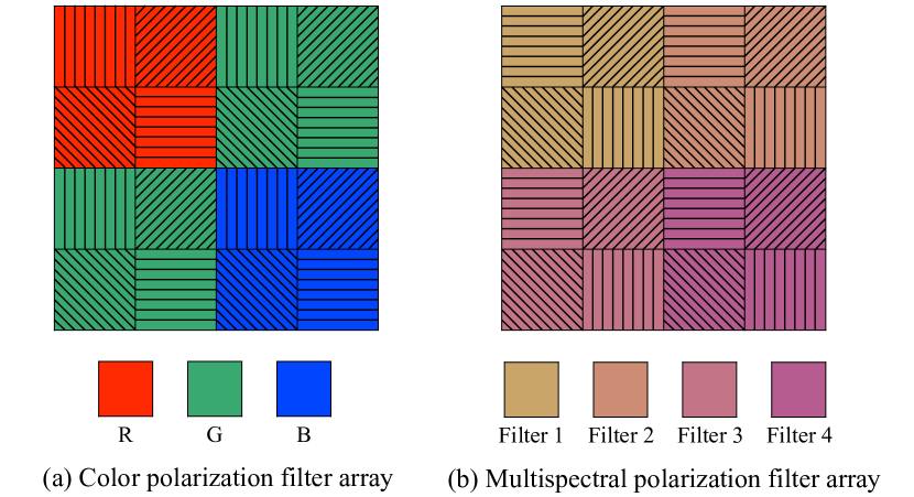
Figure 1: Filter array pattern.

On the other hand, filter array imaging, requires image reconstruction from a mosaic image in a single shot. This demosaicking process is an important step in filter array-based imaging because it strongly affects image quality. Demosaicking methods for filter array have been proposed for RGB, polarization, and color polarization imaging. Since multispectral polarization filter array have more unmeasured pixels than polarization filter array (PFA) and color polarization filter array (CPFA), a demosaicking method with higher accuracy is required.

In this study, we propose a multispectral polarization demosaicking network (MSPDNet) to improve the accuracy of multispectral polarization image reconstruction. The proposed convolutional neural network (CNN) architecture consists of a trilinear module (Tri-Module) in the trilinear interpolation layer and a multispectral module (MS-Module) in the non-linear mapping learning layer. The sparse image is generated from the mosaic image captured by snapshot multispectral polarization imaging by extracting pixel values of the same channel. The Tri-Module interpolates missing pixels by learning spatial and wavelength correlations from observed pixels in the mosaic image. The trilinear interpolation, which learns spatial and wavelength correlations, refers to values for all wavelengths, not just adjacent wavelengths. The interpolated image is refined by deep multilayer 3D convolution of the non-linear mapping learning layer. Simulation experiments showed that MSPDNet outperforms the conventional methods by 4.8 ~6.5 dB in peak signal-to-noise ratio (PSNR), and the reconstructed images are closest to the ground truth. This paper is organized as follows. Section 2 describes the related works. Section 3 presents the details of the proposed multispectral polarization demosaicking method. Section 4 presents the ablation study and a comparison with existing demosaicking methods. Section 5 presents the conclusions of this study.

2 Related works

2.1 Non-learning based demosaicking method

Many non-learning approaches have been proposed for imaging with filter array. In demosaicking polarization images, some methods [10, 11, 12, 13, 14] have been proposed to exploit the properties of polarization images with the goal of capturing a full-resolution image representing the four polarization channels (0°, 45°, 90°, and 135°). R. Wu [10] proposed a method to reconstruct three initial predictions for each missing polarization channel at a certain pixel position using different channel differences. The weights are determined by the proposed polarization channel difference prior distribution, and the edge polarization information is reconstructed. N. Li proposed a method [14] that combines Newton’s polynomial interpolation with a polarization difference model to reduce interpolation errors. The polarization difference model reduces high-frequency energy by exploiting the fact that the four polarization channels are polarization-correlated and have similar image structures.

Not only demosaicking methods of single-channel polarization images, but also a demosaicking methods of color polarization images [15, 16, 17, 18] have been proposed. These color polarization demosaics take into account the interaction between polarization and color information to improve the color reproduction accuracy of the image. M. Morimatsu [15] proposed a method based on intensity-induced residual interpolation (IGRI). The intensity guided image is generated by considering the intensity and polarization edge information in four directions. S. Qiu [16] proposed a method to solve the inverse problem of polarization mosaic model in the alternating direction method of multipliers (ADMM) framework. The Huber penalty [19] is employed as a regularization term, and physical properties are imposed as constraints to improve the reconstruction of Stokes vectors.

As a multispectral polarization demosaicking method, K. Shinoda [7] proposed a method that solves the $l_{2}$-norm minimization problem of the estimation error between the original incident light and the demosaicked image, assuming the filter array imaging as a linear model.

The disadvantage of non-learning based methods is their limited performance. Non-learning based methods have been reported to have lower demosaicking performance than learning based methods [20]. This paper [20] also discussed that many non-learning based methods are less versatile because they can only be applied to unique filter array patterns.

2.2 Learning based demosaicking method

Many CNN-based methods have been proposed for polarization demosaickings [21, 22, 23, 24] and color polarization demosaickings [25, 26, 27, 28, 29] because learning-based methods can achieve high reconstruct accuracy. M. Pistellato [22] proposed a Polarisation Filter Array Demosaicing Network (PFADN), a polarization demosaicking network consisting of two parallel branches that output the intensity and angle of linear polarization (AoLP) of unpolarized light. PFADN performs feature extraction from mosaiced images by mosaiced convolution with kernels and strides that take into account the structure of the filter array. S. C. Sargent [24] proposed a method based on conditional generative adversarial network (cGAN) [30]. This method [24] employs PatchGAN [31] as a discriminator to emphasize high-frequency components in the polarization intensity measurements and to reduce aliasing. Y. Sun [25] proposed a color polarization demosaicking convolutional neural network (CPDCNN) consisting of two branches. Branch 1 is a modified version of their previously proposed polarization demosaicking CNN (PDCNN) [23] with skip connections to reduce polarization crosstalk. Branch 2, consisting of seven dense blocks (DBs) [32], reconstructs high-frequency components from the mosaic image. For color polarization images, a color polarization filter array and its demosaicking methods [28, 29] have been proposed, in which a polarization filter is sparsely placed on a Bayer color filter and a white filter is placed in the polarization pixel area. T. Kurita [28] proposed a stokes network architecture (SNA) that compensates for low-resolution polarization information using refined RGB images as a guide.

Proposals for multispectral polarization images, which have more information in multiple dimensions than polarization images or color polarization images, are limited, and few learning-based methods exist. Learning-based methods for polarization images and color polarization images achieve sufficient accuracy even with 2D convolution, since they reconstruct one channel or three RGB channels for four polarization angles. On the other hand, multispectral polarization images reconstruct not only polarization information but also information about more wavelengths than RGB, so it is necessary to consider wavelength correlation in the learning process. Therefore, applying the network for polarization and color polarization directly to the demosaicking of a multispectral polarization image does not necessarily result in a high reconstruction. Many methods [23, 24, 25, 27] with U-net based network structures have been proposed, but they repeatedly scale the spatial resolution of the feature map by the pooling layer of the encoder and the deconvolution layer of the decoder. This scaling process does not take advantage of the spatial, wavelength, and polarization information of each pixel value in the mosaic image.

3 Proposed demosaicking method

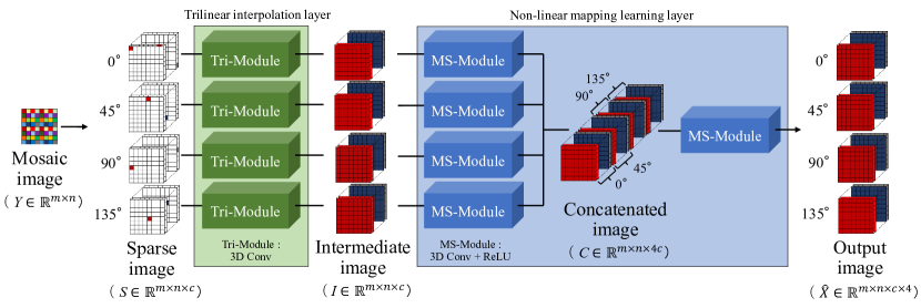
Figure 2: Architecture of the proposed MSPDNet.

In this study, we propose a demosaicking method that preserves the dimensionality of the feature map so as not to lose the observed pixel value information of the mosaic image. The proposed multispectral polarization demosaicking network (MSPDNet) is shown in the Fig. 2. The network architecture consists of a trilinear module (Tri-Module) for the trilinear interpolation layer and a multispectral module (MS-Module) for the non-linear mapping learning layer. In this paper, the mosaic image is denoted as $Y\in\mathbb{R}^{m\times n}$ ($m$, $n$ are the height and width of the image) and the demosaicked image as $\hat{X}\in\mathbb{R}^{m\times n\times c\times 4}$ ($c$ is the number of wavelengths). The sparse image $S\in\mathbb{R}^{m\times n\times c}$ is extracted from the mosaic image $Y$ for each polarization and input to the trilinear interpolation layer. The Tri-Module performs trilinear interpolation, which learns spatial and wavelength correlations by referring to values at all wavelengths. The intermediate image $I\in\mathbb{R}^{m\times n\times c}$ after trilinear interpolation is input to four parallel MS-Modules in the non-linear mapping learning layer. The MS-Module consists of a multilayer 3D convolution to extract features for each of the four polarization angles from the intermediate image $I$. Furthermore, MSPDNet inputs the concatenated image $C\in\mathbb{R}^{m\times n\times 4c}$, which is the concatenation of the outputs of the MS-Module in the wavelength direction, to the MS-Module again. The last MS-Module learns the correlation between the four polarizations based on the connected image $C$. The non-linear mapping learning layer is a deep network that concatenates MS-Module into four parallel MS-Modules. Thus, MSPDNet can learn detailed features of the multispectral polarization image and the correlation between polarizations by generating sparse images from mosaic images and by broadening and deepening the learning network.

In the following sections, section 3.1 describes the trilinear interpolation layer consisting of Tri-Modules. Section 3.2 describes the non-linear mapping learning layer consisting of the MS-Modules. Section 3.3 describes the loss function of MSPDNet.

3.1 Trilinear interpolation layer

The trilinear interpolation layer interpolates missing pixels by learning spatial and wavelength correlations from the observed pixels in the mosaic image. This trilinear interpolation refers to the values of all wavelengths, not just adjacent wavelengths.

To learn spatial and wavelength correlations, MSPDNet generates a sparse image $S\in\mathbb{R}^{m\times n\times c}$ from a mosaic image $Y\in\mathbb{R}^{m\times n}$. The mosaic image has the same spectral polarization information periodically. The sparse image is generated by extracting the pixel values of the same channel for each polarization from the mosaic image. The missing spectral information in the sparse image is set to 0. Each $m\times n$ in the sparse image has only pixel values of the same channel. The sparse images at 0°, 45°, 90°, and 135° are input to four parallel Tri-Modules in the trilinear interpolation layer. The Tri-Module consists of a single 3D convolutional layer. In the Tri-Module, the sparse image is trilinearly interpolated by kernel of 3D convolution using the correlation between wavelengths in addition to the spatial correlation of the image to obtain the intermediate image $I\in\mathbb{R}^{m\times n\times c}$. In order to use multiple observation pixels in a single convolution, it is reasonable to use a kernel size wider than the period of the filter array. Therefore, when the size of the multispectral polarization filter array is $h\times w$, the kernel size of the 3D convolution layer of Tri-Module is $(2h-1)\times(2w-1)\times c$. The first two dimensions of $(2h-1)\times(2w-1)$ are intended to utilize multiple observation pixels in a single convolution. Also, in order to learn the correlation of all wavelengths, the third dimension size of the kernel was set to $c$.

3.2 Non-linear mapping learning layer

Each intermediate image $I\in\mathbb{R}^{m\times n\times c}$ from the four Tri-Modules is input to four parallel MS-Modules in the non-linear mapping learning layer. The MS-Module learns deeper features from the intermediate image interpolated by the Tri-Module. The MS-Module is a network proposed as a demosaicking of spectral images [33], and its network structure is shown in the Fig. 3. The MS-Module has a residual network (ResNet) [34] and 3D convolution. The 3D convolution has kernel sizes of $3\times 3\times 3$ and $1\times 1\times 1$, and the number of filters is 1, 8, 16, 32, and 64. ResNet is expected to reduce errors between the demosaicked image and the training data, while 3D-CNN [35] is expected to efficiently learn local signal changes in both the spatial and spectral dimensions of the feature cube. In addition, the longest shortcut connection from the initial input to the final output effectively suppresses artifacts in demosaicked images. The outputs from the four MS-Modules are arranged wavelength-wise in the order of polarization 0°, 45°, 90°, and 135° to produce a concatenated image $C\in\mathbb{R}^{m\times n\times 4c}$, which is again given to the MS-Module.

The non-linear mapping layer first learns the wavelength correlation for each polarization from the intermediate image. The last MS-Module in the non-linear mapping layer learns not only wavelength correlation but also polarization correlation by concatenating the processed features for each polarization. The non-linear mapping layer is further deepened by concatenating the last MS-Module with four parallel MS-Modules. Additionally, since the proposed method does not have a pooling or deconvolution layer, it maintains the spatial resolution of the feature map and takes advantage of the spatial, wavelength, and polarization information of the mosaic image.

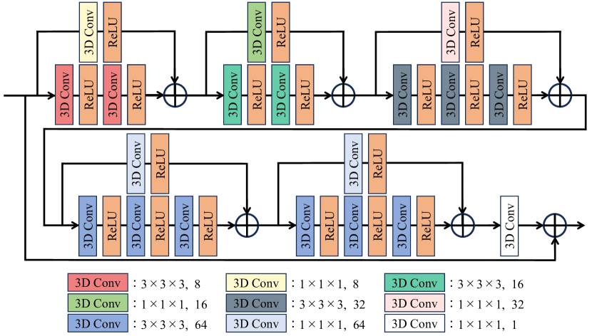
Figure 3: MS-Module architecture.

3.3 Loss function

This section describes the loss function used in MSPDNet training. The proposed loss function is designed to minimize the error between the demosaicked image and the ground truth of multispectral polarization image $X\in\mathbb{R}^{m\times n\times c\times 4}$. MSPDNet aims to learn a mapping function F() from a mosaic image $Y\in\mathbb{R}^{m\times n}$ to produce a high-quality demosaicked image. MSPDNet solves the following problems:

$$\hat{w}=\arg\min_{w}l(F(Y;w),X),$$ (1)

where $l$ denotes the loss function of MSPDNet and $w$ the network parameters.

Given the training pair $\textstyle\sum_{k=1}^{M}\left\{Y^{(k)},X^{(k)}\right\}$ (M is the number of data sets), MSPDNet learns the optimal F() that minimizes the difference between the obtained predicted value and the ground truth. The mean square error (MSE) $\textstyle\sum_{k=1}^{M}\left(\left\|X^{(k)}-F\left(Y^{(k)}\right)\right\|_{F}^{2}\right)$ is widely used to calculate the difference between predictions and ground truth. In addition to using MSE, we introduce a gradient error into the loss function that also accounts for edge errors and prevents excessive smoothing by MSE. The map obtained by calculating the first-order differential of an image in the vertical and horizontal directions is called a gradient map G. Combining MSE and gradient error, the loss function of MSPDNet can be shown as

$$l=\frac{1}{M}\sum_{k=1}^{M}\left(\left\|X^{(k)}-F\left(Y^{(k)}\right)\right\|_{F}^{2}+\lambda\left\|G_{gt}^{(k)}-G^{(k)}\right\|_{F}^{2}\right),$$ (2)

where $G\in\mathbb{R}^{m\times n\times c\times 4\times 2}$ is the gradient map, ${G_{gt}}$ is the ground truth, and $\lambda$ is the balance parameter. $\lambda$ is empirically set to 1.0.

4 Experimental results

We implemented an experiment of demosaicking in simulation with snapshot imaging using a multispectral polarization filter array. The ground truth was acquired in a system of multiple shots with a single camera, then a mosaic image was generated from the ground truth based on the pattern of the band-pass filter array. The mosaic image and the ground truth are used for demosaicking with the model trained by MSPDNet. The PSNR of the ground truth and demosaicked images are used to evaluate the image reconstruction accuracy. The effectiveness of the proposed method is confirmed by ablation study and comparison with existing methods.

4.1 Multispectral polarization dataset

Since MSPDNet training requires ground truth, multispectral polarization images were acquired by taking multiple shots with a single camera. A monochrome camera (Point Grey Grasshopper3), a lens (Nikon AI Nikkor 50mm f/1.4S), and a spectral filter (CRi VariSpec) were used in the imaging system. The spectral filter contains a linear polarizer, which was rotated at 0°, 45°, 90°, and 135° using a motorized rotor (Thorlabs K-Cube™ Brushed DC Servo Motor Controller). Two light sources (SERIC SOLAX 100W series artificial solar illuminators) were used for illumination. 20 scenes were captured with a resolution of $1800\times 1300$ pixel and a bit depth of 12 bits. The spectral information is 31 wavelengths at 10 nm intervals from 420 nm to 720 nm, and the polarization information is four polarization angles: 0°, 45°, 90°, and 135°. Fig. 4 shows a data set consisting of 20 scenes. The multispectral polarization image dataset is publicly available for research use.

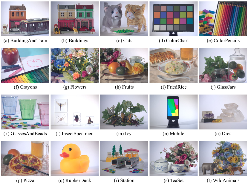
Figure 4: 20 scenes in the dataset. (http://www.is.utsunomiya-u.ac.jp/shinodalab/mspi-en.html)

4.2 Training details

The constructed multispectral polarization image dataset was used to randomly select 16 scenes for training and validation images and four scenes (in this paper, we use Fig. 4 (b), (g), (k), (n)) for test images. The training and validation images of the 16 scenes were cropped to $128\times 128$, making a total of 2,240 patches. Of the 2,240 patches, 1,960 patches were used for training and the remaining 280 patches were used for validation. For training, 16 wavelengths (420 nm to 720 nm, every 20 nm) and 4 polarization angles (0°, 45°, 90°, and 135°) were used for spectral information. First, a mosaic image is created from the dataset by passing through the multispectral polarization filter array. Fig. 5 shows a conceptual diagram of the band-pass multispectral polarization filter array set up for this simulation. The band-pass in this paper observes only the light intensity at one specific wavelength and one polarization angle. To capture a mosaic image with information on four polarization angles at 16 wavelengths, the size of the multispectral polarization filter array is $128\times 128$. It has been reported that filter arrays are advantageous for demosaicking by separating bands with close spectral bands [36, 37, 38]. Therefore, the pattern of the band-pass filter array is arranged so that consecutive bands are not adjacent to each other. Furthermore, each polarization direction (0°, 45°, 90°, 135°) is evenly spaced to collect multispectral polarization information in a balanced manner. We used Adam [39] to train MSPDNet with a learning rate of $10^{-4}$, a batch size of 1, and 50 epochs.

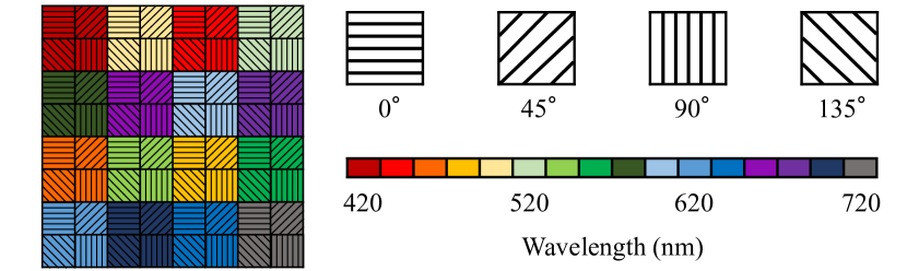
Figure 5: MSPFA of 16 wavelengths and 4 polarization angles.

4.3 Ablation study

To investigate the effectiveness of the components of MSPDNet, we compared the reconstruction accuracy with four different networks. The first network (Net1) removes the non-linear mapping learning layer from MSPDNet. The second network (Net2) changes the convolution layer of MSPDNet to a 2D convolution. The third network (Net3) removes the last MS-Module in the non-linear mapping learning layer. The fourth network (Net4) removes the gradient from the MSPDNet loss function. Net1 has 1000 epochs with a learning rate of $10^{-4}$ and a batch size of 1. Net2, Net3, and Net4 have 50 epochs each, with the same learning rate and batch size as Net1. PSNR is used as the reconstruction accuracy. The PSNR of the multispectral polarization image is the average of all polarizations at all wavelengths. In addition, the PSNR of degree of linear polarization (DoLP) is also measured. DoLP takes values between 0 and 1 and is defined by the following equation.

$$\mathrm{DoLP}=\frac{\sqrt{S_{1}^{2}+S_{2}^{2}}}{S_{0}},$$ (3)

$$\left\{\begin{array}[]{l}S_{0}=\left(I_{0^{\circ}}+I_{45^{\circ}}+I_{90^{\circ}}+I_{135^{\circ}}\right)/2\\ S_{1}=I_{0^{\circ}}-I_{90^{\circ}}\\ S_{2}=I_{45^{\circ}}-I_{135^{\circ}}\end{array},\right.$$ (4)

where $I_{\theta},\theta\in\left\{0^{\circ},45^{\circ},90^{\circ},135^{\circ}\right\}$ is the light intensity for each polarization.

Table. 1 shows the reconstruction accuracy of each network. MSPDNet has higher reconstruction accuracy than Net1, Net2, and Net3. On the other hand, there was no significant difference between Net4 and MSPDNet in the Multispectral polarization image and PSNR values. Then, the reconstructed DoLP image (720nm) is shown in Fig. 6. MSPDNet reconstructs edges more clearly than Net4, closer to ground truth. Therefore, although MSPDNet and Net4 did not differ significantly in the PSNR value of the reconstructed image, the reconstructed image of MSPDNet is visually superior to that of Net4, and the gradient error added to the loss function contributes to the improvement of the reconstruction accuracy.

Table 1: PSNR comparison of different network configurations.
(Net1 : w/o non-linear mapping learning layer, Net2 : MS-Module convolution layer to 2D, Net3 : w/o last MS-Module, Net4 : w/o gradient loss)

	Buildings		Flowers		GlassesAndBeads		Mobile		Average
Method	MSPI	DoLP	MSPI	DoLP	MSPI	DoLP	MSPI	DoLP	MSPI	DoLP
Net1	31.26	19.54	31.52	18.86	26.75	24.59	32.19	21.82	29.82	20.69
Net2	33.82	23.89	32.90	20.58	29.43	27.83	36.27	26.71	32.39	23.82
Net3	34.29	23.96	33.41	21.00	30.40	28.20	37.01	26.59	33.14	24.07
Net4	34.56	24.15	33.59	20.79	30.53	28.23	37.22	26.87	33.32	24.05
MSPDNet	34.62	24.04	33.68	20.85	30.66	28.43	37.25	26.72	33.42	24.05

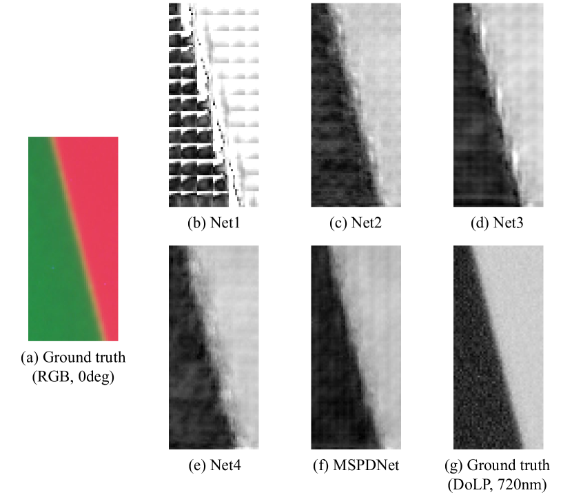
Figure 6: Demosaicked images by different network configurations.
(Net1 : w/o non-linear mapping learning layer, Net2 : MS-Module convolution layer to 2D, Net3 : w/o last MS-Module, Net4 : w/o gradient loss)

4.4 Comparison with existing demosaicking methods

We compared MSPDNet with two non-learning methods: bilinear interpolation, Wiener estimation, and two learning methods: chromatic polarization demosaicing network (CPDNet) [26], two-step color-polarization demosaicking network (TCPDNet) [27]. CPDNet and TCPDNet are color polarization demosaicking networks. CPDNet consists of a network that reconstructs RGB information from the mosaic image and then reconstructs polarization information for each wavelength using three parallel Polarization-Simulation-Modules. On the other hand, TCPDNet interpolates the mosaic image by bilinear interpolation and refines the interpolated image with a U-Net based CNN. TCPDNet consists of two steps: a four-parallel color demosaicking network and a three-parallel polarization demosaicking network. Thus, CPDNet and TCPDNet assume the reconstruction of three wavelengths (R, G, and B), resulting in three parallel networks for the reconstruction of polarization information. Since the number of wavelengths in this simulation is 16, the number of parallel networks for polarization information reconstruction is changed to 16. The number of filters in some convolutional layers was also changed to accommodate the number of parallels. For comparison, the convolution layer of the conventional methods (CPDNet and TCPDNet) was changed from 2D to 3D convolution. Since the number of datasets for the conventional methods and our proposed method is different, the number of epochs is set to 100 for CPDNet (2DConv), 2000 for CPDNet (3DConv), 10 for TCPDNet (2DConv), and 50 for TCPDNet (3DConv) based on the learning curve. The batch size for TCPDNet was changed to 1.

Table. 2 shows the PSNR values different seven methods. MSPDNet has the highest PSNR values for both the multispectral polarization image and the DoLP image. The RGB and DoLP images of the ground truth and reconstructed images are shown in Figs. 7 and 8. The red boxes in GlassesAndBeads (Figs. 7 and 8 (a)) are the areas of the patches shown in (b)~(i). An enlarged image of a portion of the image is shown in the upper left corner of each reconstructed image. Bilinear (Figs. 7 and 8 (b)) shows blur and Wiener (Figs. 7 and 8 (c)) shows block noise. CPDNet (3DConv, Figs. 7 and 8 (e)) has low color reproducibility in RGB images and does not accurately reconstruct polarization information in DoLP image. The low reconstruction accuracy of CPDNet (3DConv) could be attributed to the relatively shallow network. TCPDNet (3DConv, Figs. 7 and 8 (g)) is a deeper network than CPDNet (3DConv) and thus has higher reconstruction accuracy than CPDNet (3DConv). CPDNet (2DConv, Figs. 7 and 8 (d)) and TCPDNet (2DConv, Figs. 7 and 8 (f)) have lower reconstruction accuracy than 3DConv-based structures, indicating that wavelength correlation cannot be learned sufficiently with 2DConv-based structures. On the other hand, MSPDNet (Figs. 7 and 8 (h)) was closest to ground truth (Figs. 7 and 8 (i)) for RGB and DoLP images. To evaluate the spectral reconstruction, the root mean squared error (RMSE) of the reflectance of each spectrum with the ground truth at $S_{0}$ of the test data for each method (except CPDNet (2DConv), which has significantly lower reconstruction accuracy) is shown in Fig. 9. MSPDNet shows higher reconstruction accuracy than conventional methods in terms of spectral reconstruction. Finally, the spectral reflectance graph of $S_{0}$ for a portion of the test patch demosaicked with MSPDNet is shown in the Figs. 10 and 11. It can be seen that the spectral shape is almost identical to the original spectrum.

Table 2: PSNR comparison with conventional methods.

	Buildings		Flowers		GlassesAndBeads		Mobile		Average
Method	MSPI	DoLP	MSPI	DoLP	MSPI	DoLP	MSPI	DoLP	MSPI	DoLP
Bilinear	26.43	23.03	27.28	21.02	25.70	26.07	28.66	26.00	28.02	21.56
Wiener	30.70	21.43	32.13	19.92	28.42	25.31	24.67	21.21	26.88	23.50
CPDNet (2DConv)	17.63	18.38	17.71	17.97	14.95	18.50	16.20	14.73	16.47	17.08
CPDNet (3DConv)	32.77	23.50	31.95	20.16	21.76	25.44	34.49	25.57	26.89	23.07
TCPDNet (2DConv)	30.02	21.14	29.79	19.24	22.84	23.51	29.53	22.62	26.91	21.32
TCPDNet (3DConv)	31.96	22.13	30.96	18.73	24.52	24.67	32.53	22.57	28.65	21.48
MSPDNet	34.62	24.04	33.68	20.85	30.66	28.43	37.25	26.72	33.42	24.05

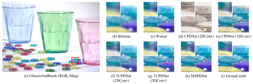
Figure 7: Demosaicked images (RGB, 0deg) of seven methods.

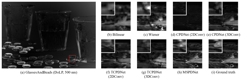
Figure 8: Demosaicked images (DoLP, 500nm) of seven methods.

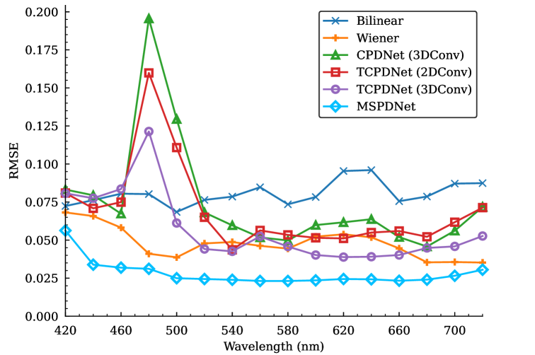
Figure 9: RMSE comparison of spectral reflectance with conventional methods.

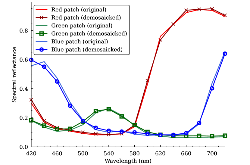
Figure 10: Reconstructed spectral reflectance.

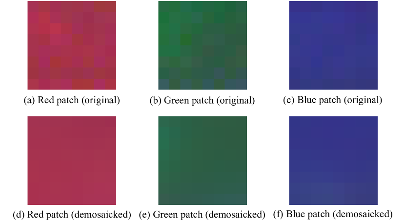
Figure 11: RGB reproduced patches with original and demosaicked reflectance.

5 Conclusion

In conclusion, we proposed MSPDNet, a demosaicking method for multispectral polarization image by deep convolution. Many conventional methods have not been able to effectively utilize the information possessed by each pixel value of the mosaic image, but MSPDNet effectively utilizes the information of spatial, wavelength, and polarization by using the sparse image as an input of the network. The reconstruction accuracy was improved by using 3D convolution and a deep and wide network of MS-Modules in parallel and series configuration. The ablation study clarified the effectiveness of the MSPDNet components. MSPDNet showed higher reconstruction accuracy than conventional methods when comparing ground-truth and demosaicked images in terms of PSNR and spectral reflectance.

By integrating this method with a multispectral polarization filter array, imaging can be performed with a single exposure, leading to downsizing of the imaging device and real-time imaging. Since MSPDNet can be applied to demosaicking various multispectral polarization filter arrays, multispectral polarization filter arrays may be incorporated in many cameras in the future. This paper is probably the first deep learning demosaicking network that can be applied to multispectral polarization filter array of four or more wavelengths, and its results are expected to lead to advances in remote sensing and medical imaging applications.

References

- [1] Siyuan Li, Jiannan Jiao, and Chi Wang. Research on polarized multi-spectral system and fusion algorithm for remote sensing of vegetation status at night. Remote Sensing, 13(17):3510, September 2021.
- [2] Ahmed EI-Habashi, Jeffrey Bowles, Deric Gray, and Malik Chami. Polarized observations for advanced atmosphere-ocean algorithms using airborne multi-spectral hyper-angular polarimetric imager. Journal of Quantitave Spectroscopy and Radiative Transfer, 262:107515, March 2021.
- [3] Sharon Gomes Ribeiro, Adunias dos Santos Teixeira, Marcio Regys Rabelo de Oliveira, Mirian Cristina Gomes Costa, Isabel Cristina da Silva Araújo, Luis Clenio Jario Moreira, and Fernando Bezerra Lopes. Soil organic carbon content prediction using soil-reflected spectra: A comparison of two regression methods. Remote Sensing, 23(13):4752, November 2021.
- [4] Y. Zhao, L. Zhang, D. Zhang, and Q. Pan. Object separation by polarimetric and spectral imagery fusion. Computer Vision and Image Understanding, 8(123), September 2009.
- [5] Brett Hooper, B. Baxter, C. C. Piotrowski, J. Z. Williams, and J. P. Dugan. An airborne imaging multispectral polarimeter. OCEANS 2009, (11154981):1–10, October 2009.
- [6] Jihwan Kim and Michael J. Escuti. Snapshot imaging spectropolarimeter utilizing polarization gratings. Optical Engineering + Applications, page 708603, August 2008.
- [7] Kazuma Shinoda, Yasuo Ohtera, and Madoka Hasegawa. Snapshot multispectral polarization imaging using a photonic crystal filter array. Optcs Express, 26(12):15948–15961, June 2018.
- [8] Tianxin Wang, Shuai Wang, Bo Gao, Chenxi Li, and Weixing Yu. Design of mantis-shrimp-inspired multifunctional imaging sensors with simultaneous spectrum and polarization detection capability at a wide waveband. Sensors, 5(24):1689, March 2024.
- [9] Jiang Shun, Li Jinzhao, Li Junyu, Lai Jianjun, and Yi Fei. Metamaterial microbolometers for multi-spectral infrared polarization imaging. Optics Express, 30(6):9065, March 2022.
- [10] Roungyuan Wu, Yongqiang Zhao, Ning LI, and Seong G. Kong. Polarization image demosaicking using polarization channel difference prior. Optics Express, 14(29):22066, July 2021.
- [11] Ashfaq Ahmed, Xiaojin Zhao, Viktor Gruev, Junchao Zhang, and Amine Bermak. Residual interpolation for division of focal plane polarization image sensors. Optics Express, 9(25), May 2017.
- [12] Junchao Zhang, Haibo Luo, Rongguang Liang, Ashfaq Ahmed, Xiangyue Zhang, Bin Hui, and Zheng Chang. Sparse representation-based demosaicing method for microgrid polarimeter imagery. Optics Letters, 43(14), July 2018.
- [13] Shumin Liu, Jiajia Chen, Yuan Xun, and Xiaojin Zhao. A new polarization image demosaicking algorithm by exploiting inter-channel correlations with guided filtering. IEEE Transactions on Image Processing, 29, 2020.
- [14] Ning Li, Yongqiang Zhao, Quan Pan, and Seong G. Kong. Demosaicking dofp images using newton’s polynomial interpolation and polarization difference model. Optics Express, 27(2):1376–1391, January 2019.
- [15] Miki Morimatsu, Yusuke Monno, Masayuki Tanaka, and Masatoshi Okutomi. Monochrome and color polarization demosaicking using edge-aware residual interpolation. arXiv:2007.14292, 2020.
- [16] Simeng Qiu, Qiang Fu, Congli Wang, and Wolfgang Heidrich. Linear polarization demosaicking for monochrome and colour polarization focal plane arrays. Computer Graphics Forum, 40(6), September 2021.
- [17] Sijia Wen and Yinqiang Zheng. A sparse representation based joint demosaicing method for single-chip polarized color sensor. IEEE Transactions on Image Processing, (30), 2021.
- [18] Lei Yan, Kaiwen Jiang, Yi Lin, Hongying Zhao, Ruihua Zhang, and Fangang Zeng. Polarized intensity ratio constraint demosaicing for the division of a focal-plane polarimetric image. Remote Sensing, 14(14), July 2022.
- [19] Huber and Peter J. Robust estimation of a location parameter. The Annals of Mathematical Statistics, 35(1):73–101, 1964.
- [20] Stojkovic Ana, Shopovska Ivana, Luong Hiep, Aelterman Jan, Jovanov Ljubomir, and Philips Wilfried. The effect of the color filter array layout choice on state-of-the-art demosaicing. Sensors, 19(14):3215, July 2019.
- [21] Xianglong Zeng, Yuan Luo, Xiaojing Zhao, and Wenbin Ye. An end-to-end fully-convolutional neural network for division of focal plane sensors to reconstruct s0, dolp, and aop. Optcs Express, 27(6):8566–8577, March 2019.
- [22] Mara Pistellato, Filippo Bergamasco, Tehreem Fatima, and Andrea Torsello. Deep demosaicing for polarimetric filter array cameras. IEEE Transactions on Image Processing, 31:2017–2026, February 2022.
- [23] Junchao Zhang, Jianbo Shao, Haibo Luo, Xiangyue Zhang, Bin Hui, Zheng Chang, and Rongguang Liang. Learning a convolutional demosaicing network for microgrid polarimeter imagery. Optics Letters, 43(18):4534–4537, September 2018.
- [24] Sargent, Garrett C., Bradley M. Ratliff, and Vijayan K. Asari. Conditional generative adversarial network demosaicing strategy for division of focal plane polarimeters. Optics Express, 25(28):38419, December 2020.
- [25] Yuanyuan Sun, Junchao Zhang, and Rongguang Liang. Color polarization demosaicking by a convolutional neural network. Optics Letters, 46(17):4338–4341, September 2021.
- [26] Sijia Wen, Yinqiang Zheng, Feng Lu, and Qinping Zhao. Convolutional demosaicing network for joint chromatic and polarimetric imagery. Optics Letters, 44(22):5646–5649, November 2019.
- [27] Vy Nguyen, Masayuki Tanaka, Yusuke Monno, and Masatoshi Okutomi. Two-step color-polarization demosaicking network. 2022 IEEE International Conference on Image Processing (ICIP), (22623880):16–19, October 2022.
- [28] Teppei Kurita, Yuhi Kondo, Legong Sun, and Yusuke Moriuchi. Simultaneous acquisition of high quality rgb image and polarization information using a sparse polarization sensor. 2023 IEEE/CVF Winter Conference on Applications of Computer Vision (WACV), pages 178–188, Januray 2023.
- [29] Liu Ju, Jin Duan, Youfei Hao, Guangqiu Chen, Hao Zhang, and Yue Zheng. Polarization image demosaicing and rgb image enhancement for a color polarization sparse focal plane array. Optics Express, 14(31):23475, July 2023.
- [30] Phillip Isola, Jun-Yan Zhu, Tinghui Zhou, and Alexei A. Efros. Image-to-image translation with conditional adversarial networks. IEEE Conference on Computer Vision and Pattern Recognition, pages 5967–5976, 2017.
- [31] Phillip Isola, Jun-Yan Zhu, Tinghui Zhou, and Alexei A. Efros. Image-to-image translation with conditional adversarial networks. Proceedings of the IEEE Conference on Computer Vision and Pattern Recognition, pages 1125–1134, 2017.
- [32] Huang Gao, Liu Zhuang, Van Der Maaten Laurens, and Weinberger Kilian Q. Densely connected convolutional networks. IEEE Conference on Computer Vision and Pattern Recognition, pages 2261–2269, 2017.
- [33] Kazuma Shinoda, Shoichiro Yoshiba, and Madoka Hasegawa. Deep demosaicking for multispectral filter arrays. arXiv, October 2018.
- [34] Kaiming He, Xiangyu Zhang, Shaoqing Ren, and Jian Sun. Deep residual learning for image recognition. Proceedings of the IEEE Computer Society Conference on Computer Vision and Pattern, pages 770–778, June 2016.
- [35] Haokui Zhang Ying Li and Qiang Shen. Spectral-spatial classification of hyperspectral imagery with 3d convolutional neural network. Remote Sensing, 9(1):67, January 2017.
- [36] Lidan Miao and Hairong Qi. The design and evaluation of a generic method for generating mosaicked multispectral filter arrays. IEEE Trans. on Image Process., 15(9):2780–2791, September 2006.
- [37] Kazuma Shinoda, Yudai Yanagi, Yoshio Hayasaki, and Madoka Hasegawa. Multispectral filter array design without training images. Optical Review, 24(4):554–571, August 2017.
- [38] Kazuma Shinoda. Unsupervised design for broadband multispectral and polarization filter array patterns. Applied Optics, 62(27):7145, September 2023.
- [39] Diederik P. Kingma and Jimmy Ba. Adam: A method for stochastic optimization. In International Conference on Learning Representations, page 44939, May 2015.