Fermi-Liquid Theory for Unconventional Superconductors
Published in “Strongly Correlated Electronic Materials - The Los Alamos Symposium 1993”, K. Bedell, Z. Wang, D. Meltzer, A. Balatsky and E. Abrahams, eds., Addison-Wesley Publishing Co., New York (1994). ISBN 0-2-1-40930-5.

Abstract

Fermi liquid theory is used to generate the Ginzburg-Landau free energy functionals for unconventional superconductors belonging to various representations. The parameters defining the GL functional depend on Fermi surface anisotropy, impurity scattering and the symmetry class of the pairing interaction. As applications I consider the basic models for the superconducting phases of UPt₃. Two predictions of Fermi liquid theory for the two-dimensional representations of the hexagonal symmetry group are (i) the zero-field equilibrium state exhibits spontaneously broken time-reversal symmetry, and (ii) the gradient energies for the different 2D representations, although described by a similar GL functionals, are particularly sensitive to the orbital symmetry of the pairing state and Fermi surface anisotropy.

I Introduction

The heavy fermions and cuprates represent classes of strongly correlated metals in which the mechanism responsible for superconductivity is probably electronic in origin. In the heavy fermions the metallic state develops below a coherence temperature $T^{*}\sim 10\,K$, well below the Debye temperature. Heavy electronic quasiparticles have Fermi velocities comparable to the sound velocity. Thus, Migdal’s expansion in $c_{s}/v_{f}$, which is the basis for the theory of conventional strong-coupling superconductors, breaks down. Overscreening of the Coulomb interaction by ions is suppressed, leaving strong, short-range Coulomb interactions to dominate the effective interaction between heavy electron quasiparticles. Phonon-mediated superconductivity is possible, but the breakdown of the Migdal expansion favors electronically driven superconductivity, or requires an electron-phonon coupling that is strongly enhanced by electronic correlations.¹ Similarly, for high $T_{c}$ materials there is no ‘theorem’ precluding superconductivity at $T_{c}\sim\,100\,K$ from the electron-phonon interaction, but the existence of high transition temperatures has often been given as reason enough for abandoning phonons as the mechanism for superconductivity in the cuprates.² Indeed much of the theoretical effort in trying to understand the origin of superconductivity in the cuprates is devoted to models based on electronic mechanisms of superconductivity (c.f. these proceedings).

An important consequence of many electronic models for superconductivity is that they often favor a superconducting state with an unconventional order parameter, i.e.  a pair amplitude that spontaneously breaks one or more symmetries of the metallic phase in addition to gauge symmetry. An order parameter with lower symmetry than the normal metallic phase can lead to dramatic effects on the superconductivity and low-lying excitation spectrum. The gap in the quasiparticle excitation spectrum may vanish at points or lines on the Fermi surface, reflecting a particular broken symmetry. Such nodes are robust features of the excitation spectrum that lead to power law behavior as $T\rightarrow 0$ for Fermi-surface averaged thermodynamic and transport properties. These average properties have been the focus of a considerable experimental and theoretical effort in order to identify the nature of the order parameter, particularly in the heavy fermion superconductors.³

However, the most striking differences between conventional and unconventional superconductors are those properties that exhibit a broken symmetry, or reveal the residual symmetry, of the order parameter. Examples of properties are (i) spontaneously broken rotational symmetries exhibited by the anisotropy of the penetration depth tensor in tetragonal, hexagonal and cubic lattice structures, (ii) new types of vortices also reflecting broken symmetries of the ordered phases, (iii) new collective modes of the order parameter that are distinct from the phase and amplitude mode in conventional superconductors, (iv) sensitivity of the superconductivity to non-magnetic impurity and surface scattering, (v) anomalous Josephson effects associated of combined gauge-rotation symmetries of the order parameter, and (vi) complex phase diagrams associated with superconducting phases with different residual symmetries. Indeed, the strongest evidence for unconventional superconductivity in metals is the multiple superconducting phases of $(U,Th)Be_{13}$ and $UPt_{3}$.^4,5 For further discussion of these issues see the reviews by Gorkov,⁶ Sigrist and Ueda,⁷ and Muzikar, et al. ⁸

At this workshop I summarized experimental evidence for, and theoreticial interpretations of, unconventional superconductivity in the heavy fermion superconductor. I focussed on UPt₃ because its complex phase diagram leads to strong constraints on the symmetry of superconducting order parameter. Another reason is that superconductivity onsets at $T_{c}\sim 0.5\,K\ll T^{*}\sim 10\,K$, in the well-developed Fermi-liquid. This separation in energy scales is important for formulating a theory of superconductivity in strongly correlated Fermion systems with predictive power. In this article I discuss the theoretical framework that supports the phenomenology on unconventional superconductivity in UPt₃ that I presented at the workshop.

The heavy fermion metals, high-$T_{c}$ cuprates and liquid ³He are strongly correlated fermion systems for which we do not have a practical first-principals theory of superconductivity and superfluidity. However, we have powerful and successful phenomenological theories for superconductivity in such systems: the Ginzburg-Landau theory and the Fermi-liquid theory of superconductivity. The full power of these phenomenological theories is realized in there connection to one another and to the experimental data on low energy phenomena. The Fermi-liquid theory of superconductivity reduces to GL theory in the limit $T\rightarrow T_{c}$, with specific predictions for the material parameters in terms of those of Fermi-liquid theory, e.g.  the Fermi surface, Fermi velocity, electronic density of states, electronic interactions, mean-free path, etc. Fermi-liquid theory then extends beyond the range of the GL theory, to low-temperatures, higher fields, and shorter wavelengths. In what follows I develop the Fermi-liquid theory of strongly correlated metals and derive the GL functionals for superconductors with an unconventional order parameter. As applications I examine the basic models for the superconducting phases of UPt₃.⁹

In Section II I summarize the GL theory for superconductors with an unconventional order parameter, and construct free energy functionals for several models of superconductivity in the heavy fermion superconductors. Section III deals with the formulation of Fermi-liquid theory for strongly correlated metals from microscopic theory. I start with the stationary free-energy functional of Luttinger and Ward,¹⁰ then formulate the Fermi-liquid theory in terms of an expansion in the low-energy, long-wavelength parameters represented by $\mbox{\sl small}\sim T/T^{*}$, $\Delta/T^{*}$, $1/k_{f}\xi_{0}$, etc. For inhomogeneous superconducting states the central equation of the Fermi-liquid theory is the quasiclassical transport equation, which generalizes the Boltzmann-Landau transport equation to superconducting Fermi liquids. External fields couple to the quasiparticle excitations and enter the transport equation through the self energy. The leading order self-energies describe impurity scattering, electron-electron interactions and the coupling to external magnetic fields. The resulting stationary free energy functional, due to Rainer and Serene,¹¹ combined with the leading order self energies, is the basis for derivations the GL theory from Fermi-liquid theory.

Material parameters are calculated for the 2D representations that have been discussed for UPt₃. An important prediction of the leading order Fermi-liquid theory, for any of the 2D representations in uniaxial superconductors, is that the equilibrium state in zero field spontaneously breaks time-reversal symmetry. The result is robust; it is independent of the details of the Fermi surface anisotropy, the basis functions determining the anisotropic gap function, as well as s-wave impurity scattering.

Extensions of the theory to low-temperature properties are also discussed. The linearized gap equation, with both diamagnetic and paramagnetic contributions, for odd-parity superconductors with strong spin-orbit coupling is examined. The gradient terms of the GL free-energy functional are related to Fermi-surface averages of products of the Fermi velocity and the pairing basis functions. These coefficients differ substantially for the various 2D representations, even though the phenomenological GL functionals of all the 2D representations are formally the same. The effects of Fermi surface anisotropy on the gradient coefficients are calculated for order parameters belonging to the E_1u and E_2u representations of $D_{6h}$ (appropriate for UPt₃). All of these results have implications for models of the superconducting phases of UPt₃, and perhaps other heavy Fermion superconductors.⁹

II Ginzburg-Landau Theory

Landau’s theory of second-order phase transitions is very general; the structure of the theory is determined principally by symmetry and a few constraints on the parameters defining the theory. Its quantitative accuracy relies on the size of the pair correlation length being large compared to the atomic scale $k_{f}^{-1}$ i.e.  $1/k_{f}\xi_{0}\sim T_{c}/T^{*}<<1$, which are well satisfied in most superconductors, including many of the heavy fermions. The generality of Ginzburg-Landau (GL) theory comes at the price of restricted predictive power; the GL theory depends on phenomenological material parameters that must be determined by comparison with experiment, or from a more fundamental theory. Futhermore, different GL theories (based on order parameters with different symmetry properties) can lead to similar phase diagrams and thermodynamic properties. Nevertheless, GL theory is an essential tool for interpreting the magnetic and thermodynamic properties of superconductors, and it has been used extensively to examine the possible phases for superconductors with an unconventional order parameter.^12-19

I assume that heavy fermion superconductors, and possibly the cuprates, are all described by an equal-time pairing amplitude of the form,

$$f_{\alpha\beta}(\vec{k}_{f})\sim\left<a_{\vec{k}_{f}\alpha}a_{-\vec{k}_{f}\beta}\right>\,,$$ (1)

where $\alpha,\beta$ are spin labels of the quasiparticles. In conventional superconductors the pair amplitude has the form, $f_{\alpha\beta}(\vec{k}_{f})=f_{0}(\vec{k}_{f})\,(i\sigma_{y})_{\alpha\beta}\,$, describing pairs with total spin zero and a (complex) amplitude $f_{0}(\vec{k}_{f})$ that breaks gauge symmetry, but otherwise retains the full symmetry of the normal metal. Unconventional superconductivity occurs when the pair amplitude spontaneously breaks additional symmetries of the normal metallic state, i.e.  if there exists an operation $R\,\varepsilon\,{\bf G}$, other than a gauge transformation, for which $R*f(R^{-1}*\vec{k}_{f})\neq f(\vec{k}_{f})$; ${\bf G}$ is the space group of the normal state, combined with time-reversal and the gauge group, ${\bf G}=G_{s}\times{\cal T}\times U(1)$. I assume that translation symmetry of the normal metal is unbroken at the superconducting transition, in which case $G_{s}$ may be indentified with the symmetry group of rotations and inversions. In the heavy fermion superconductors it is generally assumed that the spin-orbit interaction is strong (on the scale of $T_{c}$) so that only joint rotations of the orbital and spin coordinates are symmetry operations.^20,12 In this case, $G_{s}$ is identified with the point group, $G_{p}$. The labels for the quasiparticle states near the Fermi level are not eigenvalues of the spin operator for electrons. Nevertheless, in zero-field the Kramers degeneracy guarantees that each $\vec{k}$ state is two-fold degenerate, and thus, may be labeled by a pseudo-spin quantum number $\alpha$, which can take on two possible values. Furthermore, the degeneracy of each $\vec{k}$-state is lifted by a magnetic field, which is described by a Zeeman energy that couples the magnetic field to the pseudo-spin with an effective moment that in general depends on the orientation of the magnetic field relative to crystal coordinates, and possibly the wavevector $\vec{k}$. In the opposite limit of negligible spin-orbit coupling the normal state is separately invariant under rotations in spin space, so $G_{s}=SO(3)_{spin}\times G_{p}$.

Fermion statistics of the quasiparticles requires the pair amplitude to obey the anti-symmetry condition,

$$f_{\alpha\beta}(\vec{k}_{f})=-f_{\beta\alpha}(-\vec{k}_{f})\,.$$ (2)

If the normal metal has inversion symmetry, then ${\bf G}$ contains the two-element subgroup $(1,{\cal C}_{i})$. This is the case for nearly all systems of interest. For example, UPt₃, which is hexagonal with an inversion center, is described by the group ${\bf G}=D_{6h}\times{\cal T}\times U(1)$ for strong spin-orbit coupling, while the layered $CuO$ superconductors have tetragonal symmetry with a point group $D_{4h}$, or are weakly orthorhombic. The pairing interaction which drives the superconducting instability depends on the momenta and spins of quasiparticle pairs $(\vec{k}_{f}\alpha,-\vec{k}_{f}\beta)$ and $(\vec{k}_{f}^{\prime}\alpha,-\vec{k}_{f}^{\prime}\beta)$ and, and necessarily decomposes into even- and odd-parity sectors,

$$V_{\alpha\beta;\gamma\rho}(\vec{k}_{f},\vec{k}_{f}^{\prime}) = \sum_{\Gamma}^{even}\,V_{\Gamma}\,\sum_{i=1}^{d_{\Gamma}}\,{\cal Y}_{i}^{(\Gamma)}(\vec{k}_{f})(i\sigma_{y})_{\alpha\beta}\,{\cal Y}_{i}^{(\Gamma)}(\vec{k}_{f}^{\prime})^{*}(i\sigma_{y})_{\gamma\rho}$$ (3)

$$+ \sum_{\Gamma}^{odd}\,V_{\Gamma}\,\sum_{i=1}^{d_{\Gamma}}\,\vec{{\cal Y}}_{i}^{(\Gamma)}(\vec{k}_{f})\cdot(i\sigma_{y}\vec{\sigma})_{\alpha\beta}\,\vec{{\cal Y}}_{i}^{(\Gamma)}(\vec{k}_{f}^{\prime})^{*}\cdot(i\vec{\sigma}\sigma_{y})_{\gamma\rho}\,.$$

The interaction is invariant under the operations of the group ${\bf G}$ and decomposes into a sum over invariant bilinear products of basis functions for each irreducible representation $\Gamma$ of the point group, with both even- and odd-parity. The basis functions, $\{{\cal Y}^{(\Gamma)}_{i}(\vec{k}_{f})\}$, for the symmetry groups of the heavy fermion superconductors are tabulated in Ref. 21. Representative basis functions for the group $D_{6h}$, appropriate for UPt₃ with strong spin-orbit coupling, are given in Table I.

Table I: Basis functions for $D_{6h}$

  $\Gamma$ Even parity $\Gamma$ Odd parity ($\vec{d}||\hat{z}$) A_1g 1 A_1u $k_{z}$ A_2g $Im(k_{x}+ik_{y})^{6}$ A_2u $k_{z}Im(k_{x}+ik_{y})^{6}$ B_1g $k_{z}\,Im(k_{x}+ik_{y})^{3}$ B_1u $Im(k_{x}+ik_{y})^{3}$ B_2g $k_{z}\,Re(k_{x}+ik_{y})^{3}$ B_2u $Re(k_{x}+ik_{y})^{3}$ $E_{1g}$ $k_{z}{\matrix{k_{x}\cr k_{y}\cr}}$ E_1u $\left(\matrix{k_{x}\cr k_{y}\cr}\right)$ E_2g $\left(\matrix{k_{x}^{2}-k_{y}^{2}\cr 2k_{x}k_{y}\cr}\right)$ E_2u $k_{z}\left(\matrix{k_{x}^{2}-k_{y}^{2}\cr 2k_{x}k_{y}\cr}\right)$  

The order parameter separates into even- and odd-parity sectors:

$$f_{\alpha\beta}(\vec{k}_{f})=f(\vec{k}_{f})\,(i\sigma_{y})_{\alpha\beta}+\vec{f}(\vec{k}_{f})\cdot(i\vec{\sigma}\sigma_{y})_{\alpha\beta}\,,$$ (4)

where the even-parity (singlet) and odd-parity (triplet) order parameters have the general form,

$$f(\vec{k}_{f})=\sum_{\Gamma}^{even}\sum_{i}^{d_{\Gamma}}\,\eta_{i}^{(\Gamma)}\,{\cal Y}^{(\Gamma)}_{i}(\vec{k}_{f})\quad,\quad\vec{f}(\vec{k}_{f})=\sum_{\Gamma}^{odd}\sum_{i}^{d_{\Gamma}}\,\eta_{i}^{(\Gamma)}\,\vec{{\cal Y}}^{(\Gamma)}_{i}(\vec{k}_{f})\,.$$ (5)

There is an interaction parameter $V_{\Gamma}$ for each irreducible representation $\Gamma$. The superconducting instability is determined by the irreducible representation $\Gamma^{*}$ with the highest transition temperature, and barring accidental degeneracies, the order parameter, at least near $T_{c}$, will belong to the representation $\Gamma^{*}$.

II.1 Free Energy Functionals

In order to analyze the stability of the possible superconducting states a free-energy functional of the order parameter is needed; for temperatures close to the transition temperature this is the Ginzburg-Landau functional. The GL functional is invariant under the symmetry operations of the group ${\bf G}$ of the normal state, and is stationary at the equilibrium values of $\{\eta_{i}^{(\Gamma)}\}$ and equal to the thermodynamic potential. The general form of the GL functional is constructed from a symmetry analysis of the transformation properties of products of the order parameter and gradients of the order parameter. The procedure is well known and has been carried out for many of the possible realizations of unconventional superconductivity.⁷

The general form of the GL functional includes one quadratic invariant for each irreducible representation,

$$\Omega_{GL}=\sum_{\Gamma}^{irrep}\,\alpha_{\Gamma}(T)\,\sum_{i}^{d_{\Gamma}}(\eta_{i}^{(\Gamma)}\eta_{i}^{(\Gamma)*})+...\,.$$ (6)

The coefficients $\alpha_{\Gamma}(T)$ are material parameters that depend on temperature and pressure. Above $T_{c}$ all the coefficients $\alpha_{\Gamma}(T)>0$. The instability to the superconducting state is the point at which one of the coefficients vanishes, e.g.  $\alpha_{\Gamma^{*}}(T_{c})=0$. Thus, near $T_{c}$ $\alpha_{\Gamma^{*}}(T)\simeq\alpha^{\prime}(T-T_{c})$ and $\alpha_{\Gamma}>0$ for $\Gamma\neq\Gamma^{*}$. At $T_{c}$ the system is unstable to the development of all the amplitudes $\{\eta_{i}^{(\Gamma^{*})}\}$, however, the higher order terms in the GL functional which stabilize the system, also select the ground state order parameter from the manifold of degenerate states at $T_{c}$. In most superconductors the instability is in the even-parity, $A_{1g}$ channel. This is conventional superconductivity in which only gauge symmetry is spontaneously broken. An instability in any other channel is a particular realization of unconventional superconductivity.

There are two representative classes of GL theories; (i) those based on a single primary order parameter belonging to a higher dimensional representation of ${\bf G}$, and (ii) models based on two primary order parameters belonging to different irreducible representations which are nearly degenerate. Both types of model have been examined as models for the the multiple superconducting phases of UPt₃ and $(U,Th)Be_{13}$. The specific applications of these GL theories to the phase diagrams of UPt₃ and $UBe_{13}$ are discussed in detail elsewhere.^7,9,16,18,19

II.2 2D Representations of $D_{6h}$

Consider the 2D representation, E_2u, of hexagonal symmetry, with strong spin-orbit coupling. The GL functional is constructed from the amplitudes that parametrize $\vec{f}(\vec{k}_{f})$ in terms of the basis functions of Table I,

$$\vec{f}(\vec{k}_{f})=\hat{z}\left(\eta_{1}\,{\cal Y}_{1}(\vec{k}_{f})+\eta_{2}\,{\cal Y}_{2}(\vec{k}_{f})\right)\,.$$ (7)

The GL order parameter is then a complex two-component vector, $\vec{\eta}=(\eta_{1},\eta_{2})$, transforming according to the E_2u representation. The terms in the GL functional must be invariant under the symmetry group, $G=D_{6h}\times{\cal T}\times U(1)$, of point rotations, time-reversal and gauge transformations. The form of the GL functional, $\Omega_{GL}$, is governed by the linearly independent invariants that can be constructed from fourth-order products, $\sum\,b_{ijkl}\,\eta_{i}\eta_{j}\eta_{k}^{*}\eta_{l}^{*}$, and second-order gradient terms, $\sum\,\kappa_{ijkl}(D_{i}\eta_{j})(D_{k}\eta_{l})^{*}$, where the gauge-invariant derivatives are denoted by $D_{i}=\partial_{i}+i{2e\over\hbar c}A_{i}$. The fourth-order product $\eta_{i}\eta_{j}\eta_{k}^{*}\eta_{l}^{*}$ transforms as $(E_{2}\otimes E_{2})_{{\rm sym}}\otimes(E_{2}\otimes E_{2})_{{\rm sym}}=(A_{1}\oplus E_{2})\otimes(A_{1}\oplus E_{2})=2\,A_{1}\oplus A_{2}\oplus 3\,E_{2}$, yielding two linearly independent invariants. Similarly, the in-plane gradient $D_{i}\eta_{j}$ transforms as $E_{1}\otimes E_{2}=B_{1}\oplus B_{2}\oplus E_{1}$, which generates three second-order invariants. In addition, the c-axis gradient $D_{z}\eta_{i}$, which transforms as $E_{2}$, yields a fourth second-order invariant. The resulting GL functional then has the general form,^6,7

$$\Omega_{GL}\left[{\vec{\;\eta},\vec{A\;}}\right] = \int\limits d^{3}R\;\Big{\{}\,\alpha(T)\vec{\,\eta}\cdot\vec{\eta}^{*}+\beta_{1}\left({\vec{\,\eta}\cdot\vec{\eta}^{*}}\right)^{2}+\beta_{2}\left|{\vec{\eta}\cdot\vec{\eta}}\right|^{2}$$ (8)

$$+ \kappa_{1}\left({D_{i}\eta_{j}}\right)\left({D_{i}\eta_{j}}\right)^{*}+\kappa_{2}\left({D_{i}\eta_{i}}\right)\left({D_{j}\eta_{j}}\right)^{*}+\kappa_{3}\left({D_{i}\eta_{j}}\right)\left({D_{j}\eta_{i}}\right)^{*}$$

$$+ \kappa_{4}\left({D_{z}\eta_{j}}\right)\left({D_{z}\eta_{j}}\right)^{*}+\frac{1}{8\pi}\left\{|\vec{\partial}\times\vec{A}|^{2}-2\,\vec{H}\cdot\vec{\partial}\times\vec{A}\right\}\Big{\}}\,.$$

The last two terms represent the magnetic field energy for a fixed external field $\vec{H}$.

The coefficients of each invariant, $\{\alpha(T),\beta_{1},\beta_{2},\kappa_{1},\kappa_{2},\kappa_{3},\kappa_{4}\}$ are material parameters that must be determined from comparision with experiment or calculated from a more microscopic theory. A similar analysis follows for any of the 2D representations, and yields formally equivalent GL functionals, even though the order parameters belong to different representations. Thus, at the phenomenological level these GL theories yield identical results for the thermodynamic and magnetic properties. However, similar GL theories can differ significantly in their predictions when we determine the material parameters of the GL functional from a more fundamental theory, i.e.  the Fermi-liquid theory.

The equilibrium order parameter and current distribution are determined by the Euler-Lagrange equations,

$${{\delta\Omega_{GL}\left[{\vec{\eta},\vec{A}}\right]}\over{\delta\eta^{*}_{i}}}=0\,,\qquad\qquad{{\delta\Omega_{GL}\left[{\vec{\eta},\vec{A}}\right]}\over{\delta A_{i}}}=0\,;$$ (9)

which yield the GL differential equations for the order parameter, magnetic field and supercurrent,

$$\kappa_{123}D_{x}^{2}\eta_{1}+\kappa_{1}D_{y}^{2}\eta_{1}+\kappa_{4}D_{z}^{2}\eta_{1}+(\kappa_{2}D_{x}D_{y}+\kappa_{3}D_{y}D_{x})\eta_{2}$$

$$+2\beta_{1}\left({\vec{\eta}\cdot\vec{\eta}^{*}}\right)\eta_{1}+2\beta_{2}\left({\vec{\eta}\cdot\vec{\eta}}\right)\eta^{*}_{1}=\alpha\,\eta_{1}\,,$$ (10)

$$\kappa_{1}D_{x}^{2}\eta_{2}+\kappa_{123}D_{y}^{2}\eta_{2}+\kappa_{4}D_{z}^{2}\eta_{2}+(\kappa_{2}D_{y}D_{x}+\kappa_{3}D_{x}D_{y})\eta_{1}$$

$$+2\beta_{1}\left({\vec{\eta}\cdot\vec{\eta}^{*}}\right)\eta_{2}+2\beta_{2}\left({\vec{\eta}\cdot\vec{\eta}}\right)\eta^{*}_{2}=\alpha\,\eta_{2}\,,$$ (11)

and the Maxwell equation,

$$(\nabla\times\vec{b})_{i}=-{{16\pi e}\over{\hbar c}}Im[\kappa_{1}\,\eta_{j}\left({D_{\perp,i}\eta_{j}}\right)^{*}+\kappa_{2}\,\eta_{i}\left({D_{\perp,j}\eta_{j}}\right)^{*}+\kappa_{3}\,\eta_{j}\left({D_{\perp,j}\eta_{i}}\right)^{*}$$

$$+\,\kappa_{4}\,\delta_{iz}\eta_{j}\left({D_{z}\eta_{j}}\right)^{*}]\,,$$ (12)

which are the basis for studies of the H-T phase diagram, vortices and related magnetic properties.^22-26 I use the notation, $\kappa_{ijk...}=\kappa_{i}+\kappa_{j}+\kappa_{k}+...$, etc. Below I summarize the basic solutions to the GL theory and the significance of the material parameters defining the GL functional.

There are two possible homogeneous equilibrium states depending on the sign of $\beta_{2}$. For $-\beta_{1}<\beta_{2}<0$ the equilibrium order parameter, $\vec{\eta}=\eta_{0}(1,0)$ with $\eta_{0}=[|\alpha(T)|/2\beta_{12}]^{1/2}$, breaks rotational symmetry in the basal plane, but preserves time-reversal symmetry. The equilibrium state is rotationally degenerate; however, the degeneracy for an arbitrary rotations of $\vec{\eta}$ in the basal plane is accidental and is lifted by higher-order terms in the GL functional. There are three sixth-order invariants that contribute,

$$\delta\Omega_{6} = \int d^{3}R\,\Big{\{}\gamma_{1}\,\left|\vec{\eta}\right|^{6}+\gamma_{2}\,\left(\vec{\eta}\cdot\vec{\eta}^{*}\right)\left|\vec{\eta}\cdot\vec{\eta}\right|^{2}$$ (13)

$$+ \gamma_{3}\,\left[\left|\eta_{1}\right|^{6}-\left|\eta_{2}\right|^{6}-3\left(3\left|\eta_{1}\right|^{2}\left|\eta_{2}\right|^{2}+\eta_{1}^{2}\eta_{2}^{*2}+\eta_{1}^{*2}\eta_{2}^{2}\right)\left(|\eta_{1}|^{2}-|\eta_{2}|^{2}\right)\right]\Big{\}}\,,\quad$$

including the leading term in the anisotropy energy, which lifts the degeneracy and aligns $\vec{\eta}$ along one of six remaining degenerate directions.

For $\beta_{2}>0$ the order parameter retains the full rotational symmetry (provided each rotation is combined with an appropriately chosen gauge transformation), but spontaneously breaks time-reversal symmetry. The equilibrium state is doubly-degenerate with an order parameter of the form $\vec{\eta}_{+}=(\eta_{0}/\sqrt{2})(1,i)$ [or $\vec{\eta}_{-}=\vec{\eta}_{+}^{*}$], where $\eta_{0}=[|\alpha(T)|/2\beta_{1}]^{1/2}$. The broken time-reversal symmetry of the two solutions, $\vec{\eta}_{\pm}$, is exhibited by the two possible orientations of the internal orbital angular momentum,

$$\vec{M}_{orb}=(\kappa_{2}-\kappa_{3})\left(\frac{2e}{\hbar c}\right)\,Im\left({\vec{\eta}\times\vec{\eta}^{\,*}}\right)\sim\pm\,\hat{c}\;,$$ (14)

or spontaneous magnetic moment of the Cooper pairs. The presence of this term in the GL functional is exhibited by rewriting the gradient terms (for $\vec{H}=0$) in the form,

$$\Omega_{grad} = \int d^{3}R\,\Bigg{\{}\kappa_{1}\,[|\vec{D}_{\perp}\eta_{1}|^{2}+|\vec{D}_{\perp}\eta_{2}|^{2}]+\kappa_{4}\,[|D_{z}\eta_{1}|^{2}+|D_{z}\eta_{2}|^{2}]$$ (15)

$$+ \kappa_{23}(|D_{x}\eta_{1}|^{2}+|D_{y}\eta_{2}|^{2})$$

$$+ \frac{1}{2}\kappa_{23}\left[(D_{x}\eta_{1})(D_{y}\eta_{2})^{*}+(D_{x}\eta_{2})(D_{y}\eta_{1})^{*}+c.c.\right]$$

$$+ (\kappa_{2}-\kappa_{3})\left[\left(\frac{2e}{\hbar c}\right)(i\vec{\eta}\times\vec{\eta}^{*})\cdot(\vec{\partial}\times\vec{A})\right]\Bigg{\}}\,.$$

The coefficients of the gradient energy determine the magnitude and anisotropy of the spatial variations of the order parameter and supercurrents. The symmetry of the superconducting state depends critically on the values of the material parameters of the GL functional. One of the important predictions of Fermi-liquid theory for the GL free energy of any of the 2D reprepresentations of D_6h is that $\beta_{2}/\beta_{1}\simeq\frac{1}{2}$; thus, the zero-field equilibrium order paramater spontaneously breaks time-reversal symmetry. However, estimates of the material parameters from Fermi-liquid theory predict an orbital moment that is small, and therefore difficult to observe because of Meissner screening.^6,27

III Fermi-Liquid Theory

At low temperatures $T\ll T^{*}$) and low excitation energies ($\epsilon\ll T^{*}$) the thermodynamic and transport properties of most strongly interacting Fermion systems are determined by low-lying excitations obeying Fermi statistics. In metals these excitations, called ‘conduction electrons’ or ‘quasiparticles’, have charge $\pm|e|$, spin $\frac{1}{2}$, and even though they are described by the intrinsic quantum numbers of non-interacting electrons quasiparticles are complicated states of correlated electrons resulting from electron-electron, electron-ion, electron-impurity interactions and Fermi statistics. Fermi-liquid theory has been remarkably sucessful in describing the low-energy properties of liquid ³He and correlated metals with strong electron-electron and electron-phonon interactions, including many of the heavy fermions at temperatures below the coherence temperature $T^{*}$.

The central component of Landau’s theory of strongly correlated Fermions (Fermi-liquid theory) is a classical transport equation (Boltzmann-Landau transport equation) for the distribution function $g(\vec{k}_{f},\vec{R};\epsilon,t)$ describing the ensemble of quasiparticle states, where $\vec{k}_{f}$ is the position on the Fermi surface, $(\vec{R},t)$ is the space-time coordinates of a quasiparticle moving with momentum $\vec{k}\simeq\vec{k}_{f}$ and excitation energy $\epsilon$.

Green’s function techniques have been used to derive the Boltzmann-Landau transport equation.^28-31 These methods lead to expressions for the drift, acceleration and collision terms of self-energies describing quasiparticle-quasiparticle, quasiparticle-phonon and quasiparticle-impurity interactions. These self-energies are functionals of the quasiparticle distribution function and are defined in terms of interaction vertices between quasiparticles and other quasiparticle, phonons and impurities. These interaction vertices have a precise meaning, but their calculation from first principles is outside the reach of current many-body techniques. Thus, these interaction vertices are phenomenological material parameters which must be taken from comparison with experiment. The most important material parameters, the leading contributions to the quasiparticle self-energy, are the Fermi surface, Fermi velocity and density of states at the Fermi energy.

III.1 The Luttinger-Ward Functional

In order to derive the Ginzburg-Landau free energy functional, and its extension to low temperatures, it is useful to formulate an expression for the thermodynamic potential in terms of the many-body Green’s function. Such a functional was derived by Luttinger and Ward for normal fermion systems,¹⁰ and generalized by deDominicis and Martin³² to superfluid systems.

The starting point is the many-body theory for the one-particle Green’s function. For superfluid Fermi liquids the basic fermion field must be enlarged in order to describe particle-hole coherence of the pair condensate.³³ This is accomplished by introducing the four-component field operator, $\Psi(x)={\rm column}(\psi_{\uparrow},\psi_{\downarrow},\bar{\psi}_{\uparrow},\bar{\psi}_{\downarrow})$, and the $4\times 4$ Nambu Green’s function,

$$\hat{G}_{\mu\nu}(x,x^{\prime})=-\left<T_{\tau}\,\Psi_{\mu}(x)\bar{\Psi}_{\nu}(x^{\prime})\right>\,,\quad\mu=1,...,4\,,$$ (16)

where $x=(\vec{x},\tau)$ denotes the space-imaginary-time coordinate and $<...>$ is the grand ensemble average. The many-body theory for the Nambu Green’s function is derived in the usual way;³⁴ $\hat{G}$ satisfies a matrix Dyson equation with the $4\times 4$ self energy function $\hat{\Sigma}$ defined in terms of the skeleton expansion for $\hat{\Sigma}_{skeleton}[{G}]$. The particle-hole space representations of $\hat{\Sigma}$ and $\hat{G}$ are

$$\hat{G}=\left(\matrix{G&F\cr\bar{F}&\bar{G}}\right)\qquad\,,\qquad\hat{\Sigma}=\left(\matrix{\Sigma&\Delta\cr\bar{\Delta}&\bar{\Sigma}}\right)\,,$$ (17)

where each element is a $2\times 2$ spin matrix; $G$ is the diagonal Green’s function,

$$G_{\alpha\beta}(x,x^{\prime})=-\left<T_{\tau}\psi_{\alpha}(x)\bar{\psi}_{\beta}(x^{\prime})\right>\,,$$ (18)

and $F$ is the anomalous Green’s function,

$$F_{\alpha\beta}(x,x^{\prime})=-\left<T_{\tau}\,\psi_{\alpha}(x)\psi_{\beta}(x^{\prime})\right>\,,$$ (19)

describing the pair-condensate of a superfluid Fermi-liquid. The functions $\bar{G}$ and $\bar{F}$ are related by the symmetry relations, $\bar{G}_{\alpha\beta}(x,x^{\prime})=-{G}_{\beta\alpha}(x^{\prime},x)$ and $\bar{F}_{\alpha\beta}(x,x^{\prime})={F}_{\beta\alpha}(x^{\prime}(-\tau^{\prime}),x(-\tau))^{*}$.

The generalization of the free energy functional of Luttinger and Ward to superfluid Fermi systems is straight-forward. Consider a homogeneous system and transform to momentum and frequency variables: $({x},{x}^{\prime})\rightarrow(\vec{k},\epsilon_{n})$, where $\vec{k}$ is the wavevector and $\epsilon_{n}=(2n+1)\pi T$ are the Matsubara frequencies. In this case the generalization of the Luttinger-Ward free-energy functional is,

$$\Omega[\hat{G},\hat{\Sigma}]=-\frac{1}{2}\int\,\frac{d^{3}k}{(2\pi)^{3}}\, T \sum_{n}\,{\rm Tr_{4}}\Big{\{}\hat{\Sigma}(\vec{k},\epsilon_{n})\hat{G}(\vec{k},\epsilon_{n})$$ (20)

$$+ \ln[-\hat{G}_{0}(\vec{k},\epsilon_{n})^{-1}+\hat{\Sigma}(\vec{k},\epsilon_{n})]\Big{\}}\,+\,\Phi[\hat{G}]\,,$$

where $\hat{G}_{0}(\vec{k},\epsilon_{n})$ Green’s function for non-interacting Fermions,

$$\hat{G}_{0}(\vec{k},\epsilon_{n})^{-1}=\pmatrix{i\epsilon_{n}-\xi^{0}_{\vec{k}}&0\cr 0&-i\epsilon_{n}-\xi^{0}_{-\vec{k}}\cr}\,.$$ (21)

The log-functional is a formal representation of the power series in $\hat{\Sigma}$, and $\Phi[\hat{G}]$ is a functional which generates the perturbation expansion for the skeleton self-energy diagrams,

$$\hat{\Sigma}_{skeleton}[\hat{G}]=2\,\frac{\delta\Phi}{\delta\hat{G}^{tr}(\vec{k},\epsilon_{n})}\,.$$ (22)

Formally, $\Omega$ is a functional of both $\hat{G}$ and $\hat{\Sigma}$; the physical Green’s function and self-energy are defined by the stationarity conditions,

$$\frac{\delta\Omega}{\delta\hat{G}^{tr}(\vec{k},\epsilon_{n})}=0\quad\Rightarrow\quad\hat{\Sigma}(\vec{k},\epsilon_{n})=\hat{\Sigma}_{skeleton}[\hat{G}]\,,$$ (23)

$$\frac{\delta\Omega}{\hat{\Sigma}^{tr}(\vec{k},\epsilon_{n})}=0\quad\Rightarrow\quad\hat{G}^{-1}(\vec{k},\epsilon_{n})=\hat{G}_{0}^{-1}(\vec{k},\epsilon_{n})-\hat{\Sigma}(\vec{k},\epsilon_{n})\,.$$ (24)

The first equation identifies $\hat{\Sigma}$ with the skeleton expansion evaluated at the physical propagator, while the second stationarity condition is the Dyson equation. The key point is that $\Omega$ is equal to the thermodynamic potential when evaluated with $\hat{\Sigma}$ and $\hat{G}$ that satisfy the stationarity conditions; $\Omega(T,\mu)=\Omega[\hat{G}_{physical},\hat{\Sigma}_{physical}]$.

III.2 The Rainer-Serene Functional

Rainer and Serene¹¹ developed this formal machinery into a powerful calculational scheme for strongly correlated Fermion superfluids, and used their functional to explain the phase diagram and thermodynamic properties of superfluid ³He. Their formulation of the free energy functional is based on a classification of the contributions to the free-energy functional in terms of a set of small expansion parameters, e.g.  $T/T^{*}$, $T_{c}/T^{*}$, $1/k_{f}l$, $1/k_{f}\xi_{0}$, where $T_{c}$ (pairing energy scale), $l$ (mean free path) and $\xi_{0}=v_{f}/2\pi T_{c}$ (pair correlation length) represent the low-energy scales, and $T^{*}$ (degeneracy energy) and $k_{f}^{-1}$ (Fermi wavelength) are the high-energy scales of the nomal-metal. These ratios are small in nearly all systems of interest; in most heavy fermion superconductors $T_{c}/T^{*}\sim 10^{-1}-10^{-2}$, and in most metals this ratio is much smaller. The application of the Fermi-liquid model to the high $T_{c}$ superconductors is more problematic; however, special versions of Fermi-liquid theory, e.g.  the nearly anti-ferromagnetic Fermi-liquid model,^35,36 and the coupled-2D-Fermi-liquid model with interlayer diffusion,³⁷ are promising steps towards a theory of superconductivity in layered cuprates. In the following I develop the free-energy functional of Rainer and Serene for Fermi-liquid superconductors and derive the GL free energy functional for an anisotropic superconductors with an unconventional order parameter.

The propagator-renormalized perturbation expansion for the skeleton self-energy functional (or the $\Phi$-functional) is formulated in terms of the full Green’s function and bare vertices for the electron-electron, electron-ion, and electron-impurity interactions. Although the skeleton expansion is an exact formulation of the many-body problem, it is ill-suited for describing the low-energy properties of strongly correlated Fermions. A formulation of the many-body perturbation theory in terms of low-energy excitations (quasiparticles) can be carried out by re-organizing the perturbation expansion for the self energy (or $\Phi$-functional).

III.3 High- and low-energy scales

The idea is to separate $\hat{G}(\vec{k},\epsilon_{n})$ into low- and high-energy parts by introducing a formal scale, $\omega_{c}$, intermediate between the high-energy scale (e.g. $T^{*}$, bandwidth, etc.) and the relevant low-energy scale, e.g. $T$; i.e. $T\ll\omega_{c}<T^{*}$.^38,39 The non-interacting Green’s function is similarly divided into low- and high-energy parts,

$$\hat{G}_{0}(\vec{k},\epsilon_{n})=\Bigg{\{}\matrix{\hat{G}_{0}(\vec{k},\epsilon_{n})_{low}\quad,&|\epsilon_{n}|<\omega_{c}\,\,{\rm and}\,\,|\xi_{\vec{k}}^{0}|<\omega_{c}\cr\hat{G}_{0}(\vec{k},\epsilon_{n})_{high}\quad,&|\epsilon_{n}|\,\,{\rm or}\,\,|\xi_{\vec{k}}^{0}|>\omega_{c}}\,.$$ (25)

Within the low-energy region the bare propagator is of order $\hat{G}_{0}(\vec{k},\epsilon_{n})_{low}\sim{\sl small}^{-1}$, while the order of magnitude in the high-energy region is $\hat{G}_{0}(\vec{k},\epsilon_{n})_{high}\sim{\sl small}^{\,0}$, where ${\sl small}\sim T/E_{f}\ll 1$. Bare vertices (when combined with appropriate factors of the density of states) are of order ${\sl small}^{\,0}$. The perturbation expansion is then enlarged to include diagrams for both low-energy and high-energy propagators, ad re-organized into an expansion in terms of low-energy propagators and block vertices.^38,39,40 The block vertices sum an infinite set of diagrams composed of bare vertices and high-energy propagators. An example of a contribution to the self-energy with high- and low-energy propagators and bare vertices is shown in Fig. (1e); the self-energy diagram (1d) with the block vertex sums all high-energy processes that couple to the same topological arrangement of low-energy propagators.

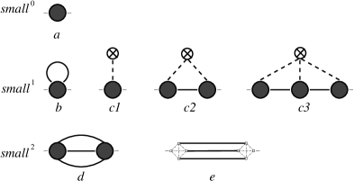
Figure 1: Leading order contributions to the quasiparticle self-energy. Block vertices couple to low-energy propagators (solid lines), and represent the summation to all orders of the bare interaction (open circle) and high-energy intermediate states (thin dotted lines).

In addition to the summation of high-energy processes into block vertices, the low-energy propagator is renormalized via the usual Dyson equation,

$$\hat{G}(\vec{k},\epsilon_{n})_{low}=\hat{G}_{0}(\vec{k},\epsilon_{n})_{low}+\hat{G}_{0}(\vec{k},\epsilon_{n})_{low}\hat{\Sigma}(\vec{k},\epsilon_{n})_{low}\hat{G}(\vec{k},\epsilon_{n})_{low}\,.$$ (26)

The low-energy part of the self energy can now be defined in terms of the set of skeleton diagrams defined as the set of $\hat{\Sigma}$ diagrams in which the self-energy insertions on internal (low-energy) propagator lines are summed to all orders by the replacement, $\hat{G}_{0}(\vec{k},\epsilon_{n})_{low}\rightarrow\hat{G}(\vec{k},\epsilon_{n})_{low}$; i.e.  $\hat{\Sigma}(\vec{k},\epsilon_{n})_{low}=\hat{\Sigma}_{skeleton}[\hat{G}_{low}]$.

The crucial assumption which makes the re-organized many-body theorytractable is that the summation of high-energy processes into block vertices does not introduce new low-energy physics that is not accounted for in the low-energy propagator and self-energy. Thus, all block vertices are estimated to be of order ${\sl small}^{\,0}$, and the renormalized low-energy propagator is assumed to be of order ${\sl small}^{-1}$. Furthermore, the block vertices, which depend on the momenta, $\vec{k}$, and energies, $\epsilon_{n}$, of the initial and final state (low-energy) excitations, are assumed to vary on the high-energy scale. Since block vertices couple only to the low-energy propagators their arguments can be evaluated with $\vec{k}\simeq\vec{k}_{f}$ and $\epsilon_{n}\simeq 0$. In addition to the order of magnitude estimates for $\hat{G}_{low}$ and the block vertices, phase space restrictions, $|\xi_{\vec{k}}|<\omega_{c}$ and $|\epsilon_{n}|<\omega_{c}$, imply the following factors,

$$T\sum_{n}^{|\epsilon_{n}|<\omega_{c}}\sim{\sl small}\quad,\quad\int_{-\omega_{c}}^{\omega_{c}}d\xi_{\vec{k}}\sim{\sl small}\,,$$

for summations and integrations over internal frequencies and momenta. These power counting rules are subject to constraints imposed by energy and momentum conservation (for details see Refs. (39)).

III.4 Leading-order theory

The leading order contributions to the low-energy electronic self-energy are shown in Fig.(1a-d). I omit the electron-phonon contributions; see Refs (39,40). The zeroth-order block vertex is the contribution to the self-energy from all high-energy processes. This term includes bandstructure and correlation effects of ion- and electron-electron interactions; the quasiparticle residue, $a(\vec{k}_{f})=(1-\partial\Sigma^{(a)}/\partial\epsilon)^{-1}$, is determined by this term. This zeroth-order self-energy term, including the quasiparticle residue, is absorbed into the renormalized quasiparticle dispersion relation, $\xi_{\vec{k}}$, and renormalized block vertices; i.e. $\xi^{0}_{\vec{k}}\rightarrow a(\vec{k})(\xi^{0}_{\vec{k}}-\Sigma^{(a)}(\vec{k}))$, and a factor of $a(\vec{k})^{1/2}$ is associated with each quasiparticle link to a block vertex.

The corrections of order ${\sl small}$ are shown as diagrams (b)-(c). Diagram (b), for the terms in particle-hole channel, corresponds to Landau’s Fermi-liquid corrections to the quasiparticle excitation energy,

$$\Sigma_{\gamma\alpha}(\vec{k})=\int\,\frac{d^{3}k^{\prime}}{(2\pi)^{3}}\,A_{\alpha\beta;\gamma\rho}(\vec{k},\vec{k}^{\prime})\,T\sum_{n^{\prime}}\,G_{\beta\rho}(\vec{k}^{\prime},\epsilon_{n^{\prime}})_{low}\,,$$ (27)

while the particle-particle channel contributes the electronic pairing energy,

$$\Delta_{\alpha\beta}(\vec{k})=\int\,\frac{d^{3}k^{\prime}}{(2\pi)^{3}}\,V_{\alpha\beta;\gamma\rho}(\vec{k},\vec{k}^{\prime})\,T\sum_{n^{\prime}}\,F_{\gamma\rho}(\vec{k}^{\prime},\epsilon_{n^{\prime}})_{low}\,.$$ (28)

The contributions to the $\Phi$-functional which generate these leading order diagonal and off-diagonal self-energies are easily constructed from eqs.(27-28),

$$\Phi^{(G)}=\frac{1}{4}\,T\sum_{n}\int\,\frac{d^{3}k}{(2\pi)^{3}}\,T\sum_{n^{\prime}}\int\,\frac{d^{3}k^{\prime}}{(2\pi)^{3}}\,G_{\gamma\alpha}(\vec{k},\epsilon_{n})_{low}\,A_{\alpha\beta;\gamma\rho}(\vec{k},\vec{k}^{\prime})\,G_{\beta\rho}(\vec{k},\epsilon_{n})_{low}\,,$$ (29)

$$\Phi^{(F)}=\frac{1}{2}\,T\sum_{n}\int\,\frac{d^{3}k}{(2\pi)^{3}}\,T\sum_{n^{\prime}}\int\,\frac{d^{3}k^{\prime}}{(2\pi)^{3}}\,F_{\alpha\beta}(\vec{k},\epsilon_{n})_{low}\,V_{\alpha\beta;\gamma\rho}(\vec{k},\vec{k}^{\prime})\,\bar{F}_{\gamma\rho}(\vec{k},\epsilon_{n})_{low}\,.$$ (30)

The functions, $A_{\alpha\beta;\gamma\rho}(\vec{k},\vec{k}^{\prime})$, and $V_{\alpha\beta;\gamma\rho}(\vec{k},\vec{k}^{\prime})$ represent the block vertices for the purely electronic interactions in the particle-hole and particle-particle channels, respectively. These ineractions may be further separated into spin-scalar and spin-vector functions for the particle-hole channel,

$$A_{\alpha\beta;\gamma\rho}(\vec{k},\vec{k}^{\prime})=A^{s}(\vec{k},\vec{k}^{\prime})\,\delta_{\alpha\gamma}\,\delta_{\beta\rho}+\vec{\sigma}_{\alpha\gamma}\cdot{\bf A}^{a}(\vec{k},\vec{k}^{\prime})\cdot\,\vec{\sigma}_{\beta\rho}\,,$$ (31)

and the spin-singlet and spin-triplet functions for the particle-particle channels,

$$V_{\alpha\beta;\gamma\rho}(\vec{k},\vec{k}^{\prime})=(i\sigma_{y})_{\alpha\beta}\,V^{(e)}(\vec{k},\vec{k}^{\prime})\,(i\sigma_{y})_{\gamma\rho}+\,(i\sigma_{y}\vec{\sigma})_{\alpha\beta}\cdot{\bf V}^{(o)}(\vec{k},\vec{k}^{\prime})\cdot(i\vec{\sigma}\sigma_{y})_{\gamma\rho}\,.$$ (32)

Thus, the singlet and triplet components of the pairing self energy become,

$$\Delta(\vec{k})=\int\,\frac{d^{3}k^{\prime}}{(2\pi)^{3}}\,V^{(e)}(\vec{k},\vec{k}^{\prime})\,T\sum_{n^{\prime}}\,F(\vec{k}^{\prime},\epsilon_{n^{\prime}})_{low}\,,$$ (33)

$$\vec{\Delta}(\vec{k})=\int\,\frac{d^{3}k^{\prime}}{(2\pi)^{3}}\,{\bf V}^{(o)}(\vec{k},\vec{k}^{\prime})\cdot\,T\sum_{n^{\prime}}\,\vec{F}(\vec{k}^{\prime},\epsilon_{n^{\prime}})_{low}\,,$$ (34)

where the singlet- and triplet-channel pairing interactions can be expanded in basis functions defined in terms of the even- and odd-parity irreducible representations of the crystal point group,

$$V^{(e)}(\vec{k},\vec{k}^{\prime})=\sum_{\Gamma}\,V_{\Gamma}\,\sum_{i}^{d_{\Gamma}}\,{\cal Y}_{i}^{(\Gamma)}(\vec{k}_{f})^{*}{\cal Y}_{i}^{(\Gamma)}(\vec{k}_{f}^{\prime})\,,$$ (35)

$${\bf V}^{(o)}(\vec{k},\vec{k}^{\prime})=\sum_{\Gamma}\,V_{\Gamma}\,\sum_{i}^{d_{\Gamma}}\,\vec{{\cal Y}}_{i}^{(\Gamma)}(\vec{k}_{f})^{*}\otimes\vec{{\cal Y}}_{i}^{(\Gamma)}(\vec{k}_{f}^{\prime})\,.$$ (36)

In addition to these mean-field electronic self-energies, impurity scattering contributes to leading order in ${\sl small}$. These terms are first-order in the impurity concentration and are collected to all orders in the quasiparticle-impurity vertex in the impurity scattering t-matrix,

$$\hat{\Sigma}_{imp}(\vec{k},\epsilon_{n})=n_{imp}\,\hat{t}(\vec{k},\vec{k};\epsilon_{n})\,,$$ (37)

where the low-energy t-matrix is given by,

$$\hat{t}(\vec{k},\vec{k}^{\prime};\epsilon_{n})=u(\vec{k},\vec{k}^{\prime})\,\hat{1}+\int\,\frac{d^{3}k^{\prime\prime}}{(2\pi)^{3}}\,u(\vec{k},\vec{k}^{\prime\prime})\,\hat{G}(\vec{k}^{\prime\prime},\epsilon_{n})_{low}\,\hat{t}(\vec{k}^{\prime\prime},\vec{k}^{\prime};\epsilon_{n})\,,$$ (38)

represents multiple scattering of low-energy excitations by the block vertex $u(\vec{k},\vec{k}^{\prime})\,\hat{1}$ for the non-magnetic quasiparticle-impurity interaction. For weak scattering the t-matrix is evaluated in second-order in the Born expansion (i.e. diagrams (c1) and (c2)). The first-order term is absorbed into $\xi_{\vec{k}}$, and the remaining piece of the impurity self-energy becomes,

$$\hat{\Sigma}_{imp}(\vec{k},\epsilon_{n})=\int\,\frac{d^{3}k^{\prime}}{(2\pi)^{3}}\,w(\vec{k},\vec{k}^{\prime})\,\hat{G}(\vec{k}^{\prime},\epsilon_{n})_{low}\,,$$ (39)

where $w(\vec{k},\vec{k}^{\prime})=n_{imp}|u(\vec{k},\vec{k}^{\prime})|^{2}$ is proportional to quasiparticle-impurity scattering probability. The corresponding contribution to the $\Phi$-functional is,

$$\Phi^{(imp)}=\frac{1}{4}\,T\sum_{n}\int\,\frac{d^{3}k}{(2\pi)^{3}}\,\int\,\frac{d^{3}k^{\prime}}{(2\pi)^{3}}\,w(\vec{k},\vec{k}^{\prime})\,Tr_{4}\,\{\hat{G}(\vec{k},\epsilon_{n})_{low}\hat{G}(\vec{k}^{\prime},\epsilon_{n})_{low}\}\,.$$ (40)

Higher order terms in ${\sl small}$ arise from electron-electron scattering (diagram (d)); this term is responsible for the inelastic quasiparticle lifetime, $1/\tau_{ee}$, and electronic strong-coupling corrections to the leading order pairing energies. The discussion that follows is confined to the leading order diagrams which define the Fermi-liquid theory of superconductivity.

The normal-state self energy, $\hat{\Sigma}_{N}$, and the propagator, $\hat{G}_{N}$, are solutions of the stationarity conditions (eqs.(23)-(24)). To leading order in ${\sl small}$ the normal-state propagator in the low-energy region is

$$\frac{1}{a}\hat{G}_{N}(\vec{k},\epsilon_{n})=\pmatrix{i\tilde{\epsilon}_{n}-\xi_{\vec{k}}&0\cr 0&-i\tilde{\epsilon}_{n}-\xi_{-\vec{k}}\cr}^{-1}\,,$$ (41)

where $\tilde{\epsilon}_{n}=\epsilon_{n}+{\rm sgn}(\epsilon_{n})/\tau$, and $\tau^{-1}=\pi N_{f}<w(\vec{k}_{f},\vec{k}_{f}^{\prime}>_{\vec{k}_{f}^{\prime}}$ is the lifetime due to impurity scattering in the normal state. Note that $<...>_{\vec{k}_{f}}$ represents the Fermi-surface average and $N_{f}$ is the density of states at the Fermi energy.

Since the pairing energy scale is of order ${\it small}$ we can construct a functional for the supercondcuting corrections to the normal-metal free energy by subtracting $\Omega_{N}=\Omega[\hat{\Sigma}_{N},\hat{G}_{N}]$ from the functional $\Omega[\hat{\Sigma}_{low},\hat{G}_{low}]$ to obtain

$$\delta\Omega\left[{\delta\hat{\Sigma},\delta\hat{G}}\right]=-{{1}\over{2}}T\sum\limits_{n}\int\limits{{d^{3}k}\over{({2\pi})^{3}}}\;Tr_{4}\;\Big{\{}\delta\hat{\Sigma}({\vec{k},\epsilon_{n}})\delta\hat{G}({\vec{k},\epsilon_{n}})\Big{\}}$$

$$-{{1}\over{2}}T\sum\limits_{n}\int\limits{{d^{3}k}\over{({2\pi})^{3}}}\;Tr_{4}\;\Big{\{}\ln^{\prime}\left[{\hat{1}-\hat{G}_{N}({\vec{k},\epsilon_{n}})\delta\hat{\Sigma}({\vec{k},\epsilon_{n}})}\right]\Big{\}}+\delta\Phi[{\delta\hat{G}({\vec{k},\epsilon_{n}})}]\ ,$$ (42)

where the $\delta\hat{\Sigma}=\hat{\Sigma}-\hat{\Sigma}_{N}$ and $\delta\hat{G}=\hat{G}-\hat{G}_{N}$ represent the superconducting corrections to the normal-state self-energy and propagator. Note that the subtracted functional contains no linear terms in $\delta\hat{\Sigma}$ or $\delta\hat{G}$ as a result of the stationarity conditions for the normal state self-energy and propagator. Thus, $\ln^{\prime}[1-x]=\ln[1-x]+x$, and the functional $\delta\Phi[\delta\hat{G}]$ is defined by

$$\delta\Phi[\delta\hat{G}]=\Phi[\hat{G}_{low}]-\Phi[\hat{G}_{N}]-\;Tr_{4}\;\Big{\{}\frac{\delta\Phi}{\delta\hat{G}^{tr}}\big{|}_{\hat{G}_{N}}\,\left(\hat{G}_{low}-\hat{G}_{N}\right)\Big{\}}\,.$$ (43)

Equation (42) for the superconducting corrections to the low-energy free energy functional, combined with the renormalized perturbation expansion in ${\sl small}$, were derived by Rainer and Serene in their work on the free energy of superfluid ³He.¹¹ This functional is used here to derive the Ginzburg-Landau free energy functional and extensions for several models of unconventional superconductivity.

III.5 Ginzburg-Landau Expansion

The free energy functional in eq. (42) depends on both the self-energies and propagators. In order to derive a free energy functional which depends only on the order parameter, it is necessary to eliminate the ‘excess’ information from the full functional. To leading order in ${\sl small}$ the stationarity condition of $\delta\Omega$ with respect to the anomalous propagator generates the mean field self-energy (gap equation) and the impurity renormalization of the gap function. The gap function provides a convenient definition of the order parameter. Reduction of the full functional to a functional of the order parameter alone is accomplished by inverting the stationarity condition relating the order parameter, $\Delta(\vec{k})$, and the anomalous propagator, $F(\vec{k},\epsilon_{n})$.

Since the mean-field self energies are independent of frequency, it is useful to introduce the frequency-summed propagator,

$$f_{\alpha\beta}({\vec{k}})=T\sum\limits_{n}\;F_{\alpha\beta}({\vec{k},\epsilon_{n}})_{low}\,.$$ (44)

Equations (33)-(34),

$$\Delta(\vec{k})=\int\frac{d^{3}k^{\prime}}{(2\pi)^{3}}\;V^{(e)}(\vec{k},\vec{k}^{\prime})f(\vec{k}^{\prime})\quad,\quad\vec{\Delta}(\vec{k})=\int\,\frac{d^{3}k^{\prime}}{(2\pi)^{3}}\,{\bf V}^{(o)}(\vec{k},\vec{k}^{\prime})\cdot\vec{f}(\vec{k}^{\prime})\,,$$ (45)

are inverted by expanding the order parameters and propagators in the basis functions that define the pairing interactions (eq.(3)), and applying the orthogonality condition,

$$\int\,d\vec{k}_{f}\,n(\vec{k}_{f})\,{\cal Y}^{\alpha(\Gamma)}_{i}(\vec{k}_{f}){\cal Y}^{\beta(\Gamma^{\prime})}_{j}(\vec{k}_{f})^{*}=\delta_{\Gamma\Gamma^{\prime}}\,\delta_{\alpha\beta}\,\delta_{ij}\,,$$ (46)

which is defined by integration over the Fermi surface with weight given by $n(\vec{k}_{f})$, the angle-resolved density of states at the Fermi surface; $\int\,d\vec{k}_{f}\,n(\vec{k}_{f})=1$. The resulting equations are,

$$\int_{-\omega_{c}}^{\omega_{c}}d\xi_{\vec{k}}\,f(\vec{k})=\sum_{\Gamma}^{even}\,\frac{1}{N_{f}V_{\Gamma}}\,\Delta^{\Gamma}(\vec{k}_{f})\quad,\quad\int_{-\omega_{c}}^{\omega_{c}}d\xi_{\vec{k}}\,\vec{f}(\vec{k})=\sum_{\Gamma}^{odd}\,\frac{1}{N_{f}V_{\Gamma}}\,\vec{\Delta}^{\Gamma}(\vec{k}_{f})\,,$$ (47)

where

$$\Delta^{\Gamma}(\vec{k}_{f})=\sum_{i=1}^{d_{\Gamma_{even}}}\,\eta^{\Gamma}_{i}\,{\cal Y}^{(\Gamma)}_{i}(\vec{k}_{f})\quad,\quad\vec{\Delta}^{\Gamma}(\vec{k}_{f})=\sum_{i=1}^{d_{\Gamma_{odd}}}\,\eta^{\Gamma}_{i}\,\vec{{\cal Y}}^{(\Gamma)}_{i}(\vec{k}_{f})\,,$$ (48)

are the order parameters belonging to even- and odd-parity representations of ${\bf G}$.

The terms in the $\delta\Phi$ functional of order small are obtained from $\Phi^{(G)}$, $\Phi^{(\bar{G})}$, $\Phi^{(F)}$ and $\Phi^{(imp)}$, and eq.(43) for $\delta\Phi$. Evaluating the $\delta\Phi$ functional at the stationary point, $\delta[\delta\Phi]/\delta[\delta\hat{G}_{low}]=0$, leads to

$$\delta\Phi=\frac{1}{4}\,T\sum\limits_{n}\int\limits{{d^{3}k}\over{\left({2\pi}\right)^{3}}}\;Tr_{4}\left\{{\delta\hat{\Sigma}(\vec{k},\epsilon_{n})\delta\hat{G}_{low}}(\vec{k},\epsilon_{n})\right\}\;,$$ (49)

where $\delta\hat{\Sigma}(\vec{k},\epsilon_{n})=\delta\hat{\Sigma}(\vec{k})_{mf}+\delta\hat{\Sigma}(\vec{k},\epsilon_{n})_{imp}$ is determined by eqs. (27)-(28) and (39). The $\delta\Phi$ contribution to the free energy functional can then be combined with the first term of eq. (42), $\delta\Omega_{1}$, to give $\delta\Omega_{1}+\delta\Phi=\frac{1}{2}\delta\Omega_{1}$. The contribution to $\delta\Omega_{1}$ coming from the diagonal self energy and propagator, although formally of order ${\sl small}^{\,2}$, vanishes at this order; thus,

$$\delta\Omega_{1}=-T\sum\limits_{n}\int\limits{{d^{3}k}\over{\left({2\pi}\right)^{3}}}\;tr\left\{{\Delta(\vec{k},\epsilon_{n})\bar{F}_{low}(\vec{k},\epsilon_{n})}\right\}\,.$$ (50)

III.6 Impurities

Elimination of the low-energy propagator is complicated by the impurity scattering contribution to $\Delta(\vec{k},\epsilon_{n})$. The probability $w(\vec{k},\vec{k}^{\prime})$ generally includes scattering in non-trivial symmetry channels. However, for point impurities (‘s-wave’ scatterers), the scattering probability can be replaced by a angle-independent scattering rate belonging to the identity representation, $N_{f}w_{0}=1/\pi\tau$. Isotropic scattering leads to considerable simplification in the reduction of $\delta\Omega[\hat{\Sigma},\hat{G}_{low}]$ to a functional of the mean-field order parameter. The order parameter is not renormalized by impurity scattering provided the scattering is in a channel other than the pairing channel. Thus, for isotropic impurity scattering any unconventional order parameter will be unrenormalized by impurity scattering,

$$\Delta_{imp}(\vec{k},\epsilon_{n})=\left<w(\vec{k}_{f},\vec{k}_{f}^{\prime})\,f(\vec{k}_{f}^{\prime},\epsilon_{n})\right>_{\vec{k}_{f}^{\prime}}\sim\frac{1}{\tau}\,\left<\Delta(\vec{k}_{f}^{\prime})\,I(\vec{k}_{f}^{\prime},\epsilon_{n})\right>_{\vec{k}_{f}^{\prime}}\,.$$ (51)

The stationary condition has been used to write $f(\vec{k},\epsilon_{n})=I(\vec{k},\epsilon_{n})\,\Delta(\vec{k}_{f})$, where $I(\vec{k},\epsilon_{n})$ is invariant under the symmetry group of the normal state. Thus, $\Delta_{imp}$ vanishes if $\Delta(\vec{k})$ belongs to any non-identity irreducible representation. As a result the impurity terms drop out of eq.(50); eliminating the frequency-summed propagator then gives,

$$\frac{1}{2}\delta\Omega_{1}=N_{f}\,\int\,d\vec{k}_{f}\,n(\vec{k}_{f})\,\Big{\{}\sum_{\Gamma}^{all}\frac{1}{N_{f}V_{\Gamma}}\,\frac{1}{2}\,tr\,\left(\Delta^{(\Gamma)}(\vec{k}_{f})\Delta^{(\Gamma)}(\vec{k}_{f})^{\dagger}\right)\Big{\}}\,,$$ (52)

where $\Delta^{(\Gamma)}(\vec{k}_{f})$ is the order parameter belonging to the representation $\Gamma$.

The remaining terms in $\delta\Omega$ come from the log-functional, and are evaluated in the GL limit by expanding in $[\hat{G}_{N}\hat{\Delta}]$ (again dropping terms higher order than ${\sl small}^{\,2}$),

$$\delta\Omega_{ln}=T\sum\limits_{n}\int\limits{{d^{3}k}\over{\left({2\pi}\right)^{3}}}\sum\limits_{m=1}^{\infty}{{\left({-1}\right)^{m}}\over{2m}}\left|{G_{N}\left({\vec{k},\epsilon_{n}}\right)}\right|^{2m}tr\left\{{(\Delta\Delta^{\dagger})^{m}}\right\}\;.$$ (53)

The resulting GL functional expanded through sixth-order in $\Delta$ becomes,

$$\Omega_{GL}\left[{\Delta}\right] = \sum\limits_{\Gamma}\alpha_{\Gamma}\left({T}\right)\left<{{1}\over{2}}tr\left({\Delta^{(\Gamma)}\Delta^{(\Gamma)\dagger}}\right)\right>+\beta_{{}_{0}}\left<{{1}\over{2}}tr\left({\Delta\Delta^{\dagger}}\right)^{2}\right>$$ (54)

$$+ \gamma_{{}_{0}}\left<{{1}\over{2}}tr\left({\Delta\Delta^{\dagger}}\right)^{3}\right>+\,...\;,$$

where the coefficients are given by,

$$\alpha_{\Gamma}(T)=N_{f}\,\Big{\{}\frac{1}{N_{f}V_{\Gamma}}-\pi T\sum_{n}^{|\epsilon_{n}|<\omega_{c}}\,\left(\frac{1}{|\epsilon_{n}|+1/\tau}\right)\Big{\}}\,,$$ (55)

$$\beta_{{}_{0}}=\frac{1}{4}N_{f}\,\pi T\sum_{n}\,\left(\frac{1}{|\epsilon_{n}|+1/\tau}\right)^{3}\quad,\quad\gamma_{{}_{0}}=-\frac{1}{8}N_{f}\,\pi T\sum_{n}\,\left(\frac{1}{|\epsilon_{n}|+1/\tau}\right)^{5}\,.$$ (56)

In the clean limit these parameters reduce to,

$$\alpha_{\Gamma}(T)=N_{f}\,\ln(T/T_{c\Gamma})\;,\;\beta_{{}_{0}}={7\zeta(3)N_{f}\over 16\,\pi^{2}T^{2}}\;,\;\gamma_{{}_{0}}=-{31\,\zeta(5)N_{f}\over 128\,\pi^{4}T^{4}}\,,$$ (57)

where $T_{c\Gamma}$ is the transition temperature of the $\Gamma$th irreducible representation; the highest $T_{c\Gamma}$ is the physical transition temperature $T_{c}$. In the vicinity of $T_{c}$, barring a near degeneracy of two irreducible representations, $\alpha_{\Gamma}$ will be positive except for the irreducible representation corresponding to $T_{c}$; thus, the order parameter will belong to a single representation near $T_{c}$.

Non-magnetic impurities are pair-breaking in unconventional superconductors. The reduction in $T_{c}$ is contained in eq. (55) for $\alpha(T)$, which can be written,

$$\alpha(T)=N_{f}\,\{\ln(T/T_{c0})+\psi(\frac{1}{2\pi\tau T}+\frac{1}{2})-\psi(\frac{1}{2})\}\,,$$ (58)

where the pairing interaction $V_{\Gamma}$ and the cutoff, $\omega_{c}$, have been eliminated in favor of $T_{c0}$, the clean-limit value for the transition temperature, and $\psi(x)$ is the di-gamma function. The equation for $T_{c}$ is given by the Abrikoso-Gorkov formula, $\ln(T_{c0}/T_{c})=\psi(\frac{1}{2\pi\tau T_{c}}+\frac{1}{2})-\psi(\frac{1}{2})$, but with $\tau$ due to non-magnetic scattering. Near $T_{c}$, $\alpha(T)\simeq\alpha^{\prime}(T-T_{c})$; impurity scattering reduces the coefficient $\alpha^{\prime}=_{f}/T_{c}\{1-\frac{1}{2\pi\tau T_{c}}\,\psi^{\prime}(\frac{1}{2\pi\tau T_{c}}+\frac{1}{2})\}$. Both $T_{c}(\tau)$ and $\alpha^{\prime}(\tau)$ vanish at the same critical value of $\tau$, $\frac{1}{2\pi\tau_{cr}T_{c0}}\sim 1$.

The impurity corrections to the higher order GL coefficients can also be expressed as functions of $\frac{1}{2\pi\tau T_{c}}$. In particular, the fourth-order coefficient is given by,

$$\beta_{{}_{0}}=\frac{N_{f}}{32\pi^{2}T_{c}^{2}}\,\left[-\psi^{\prime\prime}(\frac{1}{2\pi\tau T_{c}}+\frac{1}{2})\right]\,,$$ (59)

which reduces to eq.(57) in the clean limit. In the ‘dirty’ limit, $\frac{1}{2\pi\tau T_{c}}\rightarrow\infty$, which onsets rapidly for $\frac{1}{2\pi\tau T_{c0}}\sim 1$ since $T_{c}(\tau)$ is strongly suppressed, $\beta_{{}_{0}}^{dirty}\simeq\frac{1}{8}\tau^{2}$. Thus, impurities suppress the superconducting transition, but they do not change the order of the transition.

III.7 Two-dimensional representations

In order to proceed further it is necessary to specify the relevant pairing channel, and the general properties of the pairing interaction, particularly if an odd-parity channel is involved. The Fermi surface averages are carried out by expanding $\Delta(\vec{k}_{f})$ in the basis functions of the appropriate irreducible representation. For odd-parity representations the basis functions, and therefore the spin averages, depend on the strength of the spin-orbit interactions.

In the absence of spin-orbit coupling, the spin-triplet terms are due entirely to exchange interactions; thus, the odd-parity vertex is isotropic under separate rotations of the spin and orbital coordinates of the quasiparticles linked by the interaction vertex, i.e.  ${\bf V}^{(o)}(\vec{k},\vec{k}^{\prime})=\,{\bf 1}\,\times\,\sum_{\Gamma}^{odd}\,V_{\Gamma}\,\sum_{i=1}^{d_{\Gamma}}\,{\cal Y}_{i}^{(\Gamma)}(\vec{k}_{f}){\cal Y}_{i}^{(\Gamma)}(\vec{k}_{f}^{\prime})^{*}$. The direction of spin of the pairs represents a spontaneously broken continuous symmetry. Thus, small magnetic fields can orient the spin components of the order parameter.

By contrast, odd-parity superconductors with strong spin-orbit coupling have the spin-quantization axis determined (at least in part) by spin-orbit interactions which are large compared to the pairing energy scale, i.e.  of order ${\sl small}^{\,0}$. The general form of the basis functions, $\{\vec{{\cal Y}}^{(\Gamma)}_{i}(\vec{k}_{f})\}$, are quite complicated. However, if spin-orbit coupling selects a preferred spin quantization axis along a high-symmetry direction in the crystal, an ‘easy axis’, then the odd-parity interaction simplifies considerably.

Consider the case in which the spin quantization axis is locked to the six-fold rotation axis of a hexagonal crystal. The odd-parity interaction reduces to,

$${\bf V}^{(o)}(\vec{k},\vec{k}^{\prime})=\,\hat{z}\otimes\hat{z}\,\sum_{\Gamma}^{odd}\,V_{\Gamma}\,\sum_{i=1}^{d_{\Gamma}}\,{\cal Y}_{i}^{(\Gamma)}(\vec{k}_{f}){\cal Y}_{i}^{(\Gamma)}(\vec{k}_{f}^{\prime})^{*}\,.$$ (60)

The pairing interaction produces only pairing correlations with $\vec{\Delta}\sim\hat{z}$, i.e.  odd-parity, $S=1$ pairs with $\hat{z}\cdot\vec{S}=0$. Thus, strong spin-orbit coupling can have dramatic effect on the paramagnetic properties of odd-parity superconductors.

The GL functionals for the 1D representations are formally the same. The material parameters defining these functionals for different representations differ by minor factors of order one because of the Fermi surface averages of the basis functions for higher order invariants differ slightly. The most significant difference is the insensitivity of the identity representation to non-magnetic impurity scattering. For this case the impurity renormalization of $\Delta$ does not vanish, but cancels the impurity renormalization of the self-energy in the low-energy propagator $G_{N}(\vec{k},\epsilon_{n})$. All other 1D representations suffer from the pair-breaking effect of non-magnetic impurities.

The more interesting cases are the 2D representations with strong spin-orbit coupling. An order parameter belonging to a 2D represensentation of $D_{6h}$ has been proposed for the superconducting phases of UPt₃, and an odd-parity representation with $\vec{\Delta}\sim\hat{z}$ accounts for the anisotropy of $H_{c2}(T)$ at low temperatures (see Ref. (41) and below). Consider the odd-parity 2D representation of $D_{6h}$ with the spin quantization axis locked to $\hat{z}$ by strong spin-orbit coupling. For either $E_{1u}$ or $E_{2u}$,

$$\vec{\Delta}(\vec{k}_{f})=\hat{z}\,\left(\eta_{1}\,{\cal Y}_{1}(\vec{k}_{f})+\eta_{2}\,{\cal Y}_{2}(\vec{k}_{f})\right)\,,$$ (61)

where the orbital functions are listed in Table I. The Fermi-surface integrals are simplest in the RCP and LCP basis, ${\cal Y}_{\pm}(\vec{k}_{f})\sim\,k_{z}^{n-1}\,(k_{x}\pm ik_{y})^{n}$ for the odd-parity $E_{n}$ representation ($n=1,2$). The Fermi-surface averages for the fourth-order terms lead to the following: (i) $<|{\cal Y}_{+}|^{4}>=<|{\cal Y}_{-}|^{4}>=<|{\cal Y}_{+}|^{2}|{\cal Y}_{-}|^{2}>$, (ii) $<{\cal Y}_{+}{\cal Y}_{-}^{*}(|{\cal Y}_{+}|^{2}+|{\cal Y}_{-}|^{2})>=0$, and (iii) $<{\cal Y}_{+}^{2}{\cal Y}_{-}^{*2}>=0$. These relations and analogous relations for the sixth-order terms give the following results or the material parameters of the GL functional in eq.(8),

$$\beta_{1} = 2\beta_{2}=\beta_{{}_{0}}<|{\cal Y}_{+}(\vec{k}_{f})|^{4}>$$

$$\gamma_{1} = \frac{2}{3}\gamma_{2}=\gamma_{{}_{0}}<|{\cal Y}_{+}(\vec{k}_{f})|^{6}>\,\,,\quad\gamma_{3}=0\,.$$ (62)

There are a couple of important points to be made here. The sign of $\beta_{2}$ determines the relative stability of competing ground states; $\beta_{2}>0$ stabalizes a state with broken time-reversal symmetry of the form $\vec{\eta}\sim(1,\pm i)$. The leading order theory predicts $\beta_{2}/\beta_{1}=\frac{1}{2}$, and therefore a ground state with broken ${\cal T}$-symmetry for all of the four 2D representations with strong spin-orbit coupling. The ratio of $\frac{1}{2}$ is independent of the detailed geometry of the Fermi surface, and insensitive to impurity scattering. This latter result follows mainly from the assumption that the scattering probability is dominated by the channel corresponding to the identity representation, in which case the impurity renormalization of $\Delta(\vec{k}_{f})$ vanishes. The impurity effects completely factor out of the Fermi surface average when the scattering rate is isotropic, leaving the ratio for $\beta_{2}/\beta_{1}$ to be determined solely by symmetry. The importance of this result is two-fold: (i) the ground state of any of the 2D models exhibits broken ${\cal T}$ symmetry, and is doubly degenerate with $\vec{\eta}\sim(1,\pm i)$, and (ii) such a ground state (and therefore $\beta_{2}>0$) is a pre-requisite for explaining the double transition in zero field for UPt₃ in terms of a 2D order parameter of $D_{6h}$ coupled to a weak symmetry breaking field. These models are discussed in detail in Ref. (9). Note also that the hexagonal anisotropy energy, proportional to $\gamma_{3}$, vanishes in the leading order approximation.

The heat capacity jump at $T_{c}$ for the ground state $\vec{\eta}_{\pm}\sim\,\left(1,\pm i\right)$ is $\Delta C=\alpha^{2}/\left({2\beta_{1}T_{c}}\right)$, which in leading-order theory becomes,

$$\frac{\Delta C}{\gamma T_{c}}=\frac{24}{<|{\cal Y}_{+}(\vec{k}_{f})|^{4}>}\,\left\{\frac{(1-\frac{1}{2\pi\tau T_{c}}\,\psi^{\prime}(\frac{1}{2\pi\tau T_{c}}+\frac{1}{2}))^{2}}{-\psi^{\prime\prime}(\frac{1}{2\pi\tau T_{c}}+\frac{1}{2})}\right\}\,,$$ (63)

which depends on the specific geometry of the Fermi surface the details of the basis functions, and the pair-breaking effect of impurities. In the clean limit, $\Delta C/\gamma T_{c}=12\zeta(3)/<|{\cal Y}_{+}(\vec{k}_{f})|^{4}>$. As a rough estimate, the $E_{2u}$ basis functions with a spherical Fermi surface give a specific heat jump of $\Delta C/\gamma T_{c}\simeq 0.97$. Pair-breaking from impurity scattering leads to further reduction of the heat capacity jump.

Most heavy fermion superconductors show a specific heat jump significantly different from the value $\Delta C/\gamma T_{c}=1.43$ expected for a conventional BCS superconductor. In $UPt_{3}$ estimates of $\Delta C/\gamma T_{c}$ range from $\approx 0.33$ to $\approx 1.0$; more recent reports indicate that this spread in specific heat jumps is related to sample quality, and in the highest quality single crystals of $UPt_{3}$ (highest $T_{c}$) the specific-heat jump is $\approx 1.0$.⁴²

III.8 Quasiclassical Theory

The utility and predictive power of Fermi-liquid theory depends on the plausible, but essential, assumption that the low-energy propagator is of order ${\sl small}^{-1}$, compared to the high-energy part of the propagator and the block vertices which are of order ${\sl small}^{\,0}$, and varies on a scale small compared to the $\omega_{c}$. By contrast, the self-energy does not vary rapidly with $\xi_{\vec{k}}$. This allows a further simplification; the rapid variations of the low-energy propagator with $\xi_{\vec{k}}$, corresponding to the fast spatial oscillations of the propagator on the atomic scale of $k_{f}^{-1}$, can be integrated out of the low-energy functional. The relevant low-energy functions are the quasiclassical propagator,

$$\hat{g}(\vec{k}_{f},\epsilon_{n})=\frac{1}{a}\,\int_{-\omega_{c}}^{\omega_{c}}\,d\xi_{\vec{k}_{f}}\,\hat{\tau}_{3}\,\hat{G}(\vec{k},\epsilon_{n})_{low}\,,$$ (64)

and the quasiclassical self-energy, $\hat{\sigma}(\vec{k}_{f},\epsilon_{n})=a\,\hat{\Sigma}(\vec{k}_{f},\epsilon_{n})\hat{\tau}_{3}$, where the particle-hole matrix $\hat{\tau}_{3}$ is inserted for convenience. Products of the form $\int\,\frac{d^{3}k}{(2\pi)^{3}}\,\hat{\Sigma}(\vec{k},\epsilon_{n})\break\hat{G}(\vec{k},\epsilon_{n})_{low}$ are replaced by Fermi surface averages, $\int\,d\vec{k}_{f}\,n(\vec{k}_{f})\,\hat{\sigma}(\vec{k}_{f},\epsilon_{n})\,\hat{g}(\vec{k}_{f},\epsilon_{n})$. The advantage of $\xi_{\vec{k}}$-integrating is that the spatial variations on length scales large compared to $k_{f}^{-1}$ are easily incorporated into the low-energy theory. Such a formulation is essential for the description of inhomogeneous superconductivity, e.g. current carrying states, vortex structures, Josephson phenomena near interfaces and weak links, etc.⁴³ Indeed many of the unique properties of unconventional superconductors are connected with spatial variations of the order parameter on length scales of order $\xi_{0}=v_{f}/2\pi T_{c}$.⁴⁴

Eilenberger’s original formulation of the quasiclassical theory starts fromGorkov’s equations and integrates out the short-wavelength, high-energy structure to obtain the transport equation for the quasiclassical propagator,³⁰

$$\left[i\epsilon_{n}\hat{\tau}_{3}-\hat{\sigma}(\vec{k}_{f},\vec{R};\epsilon_{n})\,,\,\hat{g}(\vec{k}_{f},\vec{R};\epsilon_{n})\right]+i\vec{v}_{f}\cdot\vec{\nabla}\hat{g}(\vec{k}_{f},\vec{R};\epsilon_{n})=0\,.$$ (65)

In addition, the quasiclassical propagator satisfies the normalization condition,

$$\hat{g}(\vec{k}_{f},\vec{R};\epsilon_{n})^{2}=-\pi^{2}\,\hat{1}\,.$$ (66)

The generalization of the low-energy free-energy functional to include spatial variations on scales $R\gg k_{f}^{-1}$ is straight-forward; expressed in terms of the quasiclassical propagator and self-energy the Rainer-Serene functional becomes,

$$\delta\Omega\left[{\hat{g},\hat{\sigma}}\right]=-\frac{1}{2}N_{f}\int\limits d^{3}R\int\,d\vec{k}_{f}\,n(\vec{k}_{f})\,T\sum\limits_{n}Tr_{4}\Big{\{}\hat{\sigma}({\vec{k}_{f},\vec{R};\epsilon_{n}})\hat{g}({\vec{k}_{f},\vec{R};\epsilon_{n}})$$

$$+\int_{-\omega_{c}}^{\omega_{c}}\,d\xi_{\vec{k}}\;\ln\left[{-\hat{\tilde{G}}_{N}^{-1}({\vec{k},\vec{R};\epsilon_{n}})+\hat{\sigma}({\vec{k}_{f},\vec{R};\epsilon_{n}})}\right]\Big{\}}+\delta\Phi\left[{\hat{g}}\right]\;,$$ (67)

where $\hat{\tilde{G}}_{N}(\vec{k},\vec{R};\epsilon_{n})^{-1}=(i\epsilon_{n}\hat{\tau}_{3}-\xi_{\vec{k}}^{op})$ is a differential operator; $\xi_{\vec{k}}^{op}*g(\vec{k}_{f},\vec{R};\epsilon_{n})=\xi_{\vec{k}}\,g(\vec{k}_{f},\vec{R};\epsilon_{n})-\frac{i}{2}\vec{v}_{f}\cdot\vec{\nabla}g(\vec{k}_{f},\vec{R};\epsilon_{n})$. As a result the $\xi_{\vec{k}}$-integration is straight-forward only for homogeneous equilibrium. Nevertheless, this functional provides the basis for the free-energy analysis of inhomogenous superconducting states, and for $T\rightarrow T_{c}$ can be reduced to the GL functional for spatially varying configurations of the order parameter.

The stationarity condition $\delta[\delta\Omega]/\delta[\hat{\sigma}]=0$ generates the $\xi_{\vec{k}}$-integrated Dyson equation for the low-energy propagator,

$$\hat{g}({\vec{k}_{f},\vec{R};\epsilon_{n}})=\int_{-\omega_{c}}^{\omega_{c}}d\xi_{\vec{k}}\,({\hat{\tilde{G}}_{N}^{-1}-\hat{\sigma}})^{-1}\;,$$ (68)

which can be transformed into the quasiclassical transport equation (65). The transport equation and normalization condition are complete with the specification of the relevant self energy terms. In addition to the leading order self-energy terms (Fig. 1), magnetic fields couple to low-energy quasiparticles to leading order in ${\sl small}$ through the diamagnetic coupling,

$$\hat{\sigma}_{A}=\frac{e}{c}\vec{v}_{f}\cdot\vec{A}(\vec{R})\hat{\tau}_{3}\,,$$ (69)

and the Zeeman coupling,

$$\hat{\sigma}_{B}=-B_{i}(\vec{R})\,\mu_{ij}(\vec{k}_{f})\,\hat{S}_{j}\,,$$ (70)

where $\vec{B}=\vec{\nabla}\times\vec{A}$, $\hat{\vec{S}}=\frac{1}{2}(\hat{1}+\hat{\tau}_{3})\vec{\sigma}+\frac{1}{2}(\hat{1}-\hat{\tau}_{3})\vec{\sigma}^{tr}$ is the quasiparticle spin operator, and $\mu_{ij}(\vec{k}_{f})$ is the effective moment; for a uniaxial crystal with strong spin-orbit coupling $\mu_{ij}\rightarrow{\rm diag}\,(\mu_{\perp},\mu_{\perp},\mu_{||})$. The vertex for the diamagnetic coupling is $\frac{e}{c}\vec{v}_{f}$, which follows from gauge invariance.

III.9 Linearized Gap Equation

In the following I use the quasiclassical equations to derive the linearized gap equation for the upper critical field, including the paramagnetic corrections, and obtain the gradient coefficients of the GL functional for odd-parity, 2D representations of $D_{6h}$. Near the second-order transition line ($\Delta/T_{c}\rightarrow 0$) the quasiclassical equations may be linearized in $\Delta$; the diagonal propagator is given by its normal-state value,

$$\hat{g}_{N}(\vec{k}_{f},\vec{R};\epsilon_{n})=-i\pi\,{\rm sgn}(\epsilon_{n})\,\hat{\tau}_{3}\,,$$ (71)

while the linear correction is determined by the differential equation,

$$i\vec{v}_{f}\cdot\vec{D}f+2i\tilde{\epsilon}_{n}f+\mu(\vec{\sigma}\cdot\vec{B}\,f+f\,\sigma_{y}\vec{\sigma}\sigma_{y}\cdot\vec{B})=2i\pi\,{\rm sgn}(\epsilon_{n})\,\Delta(\vec{k}_{f},\vec{R};\epsilon_{n})\,,$$ (72)

where the diamagnetic coupling is combined with the derivative, $\vec{D}=\vec{\nabla}+i\frac{2e}{c}\vec{A}$ , $\tilde{\epsilon}_{n}=\epsilon_{n}+{\rm sgn}(\epsilon_{n})/\tau$ includes isotropic impurity scattering, and I assume an isotropic effective moment, $\mu$.

For an odd-parity representation the upper critical field is determined by the the linearized gap equation,

$$\vec{\Delta}(\vec{k}_{f},\vec{R})=N_{f}\int d\vec{k}_{f}^{\prime}\,{\bf V}(\vec{k}_{f},\vec{k}_{f}^{\prime})\cdot\,2\pi T\sum_{n}\int_{0}^{\infty}ds\exp\{-2s|\epsilon_{n}|-{\rm sgn}(\epsilon_{n})\,s\,\vec{v}_{f}^{\prime}\cdot\vec{D}\}$$

$$\left[1+\left(\cos(2s\mu B)-1\right)\hat{\bf h}\otimes\hat{\bf h}\right]\,\vec{\Delta}(\vec{k}_{f}^{\prime},\vec{R})\,,\quad$$ (73)

where I have specialized to the clean limit, and $\hat{\bf h}$ is the direction of the field. Note that the paramagnetic effect drops out of the gap equation for any odd-parity representation with $\vec{\Delta}\perp\vec{B}$. In the case of strong spin-orbit coupling with the quantization axis locked to $\hat{z}$, i.e. ${\bf V}=\hat{z}\otimes\hat{z}\,V_{\Gamma}\,{\cal Y}^{(\Gamma)}(\vec{k}_{f}){\cal Y}^{(\Gamma)}(\vec{k}_{f}^{\prime})^{*}$, the paramagnetic limiting of the upper critical field is strongly anisotropic, and vanishes for $\vec{B}\perp\hat{z}$. Choi and I argued that the strong anisotropy of $H_{c2}$ at low temperatures in UPt₃ is evidence for this type of pairing; i.e. odd-parity, with $\vec{\Delta}\sim\hat{z}$ locked by spin-orbit coupling.⁴¹

The anisotropy of the paramagnetic effect is also observable in the GL region. The Zeeman coupling contributes a term in the GL functional of the form,

$$\Omega_{Zeeman}=g_{z}\,\int d^{3}R\,|\vec{B}\cdot\vec{z}|^{2}\,\left(|\eta_{1}|^{2}+|\eta_{2}|^{2}\right)\,,$$ (74)

where the g-factor is determined by the effective moment,

$$g_{z}={7\zeta(3)}\frac{N_{f}\mu^{2}}{4\pi^{2}T_{c}^{2}}\,.$$ (75)

The important point is that the Zeeman energy is pair-breaking for $\vec{B}||\hat{z}$, but not for $\vec{B}\perp\hat{z}$. Thus, if $\vec{\Delta}||\hat{z}$ is enforced by strong spin-orbit coupling, then $H^{||}_{c2}(T)$ is suppressed by the Zeeman effect at low-temperatures, while the temperature dependence of $H_{c2}^{\perp}$ is determined only by diamagnetism; the paramagnetic terms drop out for this field orientation since the field merely shifts the population of Cooper pairs with spin directions $|\Leftarrow>$ and $|\Rightarrow>$, without any loss of condensation energy. The effects of impurity scattering on both even- and odd-parity superconductors is discussed in Ref.(45).

III.10 Gradient Coefficients for the 2D Representations of $D_{6h}$

Although the phenomenological GL theories are formally the same for any of the 2D representations, the predictions for the GL material parameters may differ substantially depending on the geometry of the Fermi surface and symmetry of the Cooper pair basis functions. For instance, for the homogeneous terms in the GL functional, the fourth-order free energy coefficients have the ratio, $\frac{\beta_{2}}{\beta_{1}}=\frac{1}{2}$ to leading order in ${\sl small}$ for any of the four 2D representations; this result is insensitive to hexagonal anisotropy of the Fermi surface and basis functions, and to non-magnetic, s-wave impurity scattering.

Significant differences between the 2D representations appear when one considers the gradient terms in the GL functional. In order to calculate the leading order gradient terms in the GL equation consider the linearized gap equation (73). Near $T_{c}$ the estimates $|\epsilon_{n}|\sim T_{c}$, $|\vec{v}_{f}\cdot\vec{D}|\sim T_{c}\sqrt{1-T/T_{c}}$ apply, so that to leading order in $\sqrt{1-T/T_{c}}$ the linearized equation for the odd-parity gap function becomes,

$$\vec{\Delta}(\vec{k}_{f},\vec{R})=\int\,d^{2}\vec{k}_{f}^{\prime}\,n(\vec{k}_{f}^{\prime})\,V(\vec{k}_{f},\vec{k}_{f}^{\prime})\left\{{\cal K}(T)+\frac{7\zeta(3)}{16\pi^{2}T_{c}^{2}}\,(\vec{v}_{f}^{\prime}\cdot\vec{D})^{2}\right\}\,\vec{\Delta}(\vec{k}_{f}^{\prime},\vec{R})\,,$$ (76)

where ${\cal K}(T)=\ln(1.13\,\omega_{c}/T)$. The same equation holds for the even-parity channel with appropriate substitutions for the gap function and pairing interaction. This equation is used to generate the coefficients of the gradient terms in the GL equations. For any of the even-parity, or odd-parity (with $\vec{\Delta}||\hat{z}$), 2D models the gradient coefficients become,

$$\kappa_{1} = \kappa_{0}\,\left<{\cal Y}_{1}(\vec{k}_{f})\,v_{fy}\,v_{fy}\,{\cal Y}_{1}(\vec{k}_{f})\right>$$

$$\kappa_{2} = \kappa_{3}=\kappa_{0}\,\left<{\cal Y}_{1}(\vec{k}_{f})\,v_{fx}\,v_{fy}\,{\cal Y}_{2}(\vec{k}_{f})\right>$$

$$\kappa_{4} = \kappa_{0}\,\left<{\cal Y}_{1}(\vec{k}_{f})\,v_{fz}\,v_{fz}\,{\cal Y}_{1}(\vec{k}_{f})\right>\,,$$ (77)

where ${\cal Y}_{i}(\vec{k}_{f})$ are the basis functions and $\kappa_{0}=\frac{7\zeta(3)}{16\pi^{2}T_{c}^{2}}\,N_{f}$. There are important differences between the E₁ and E₂ representations when we evaluate these averages for the in-plane stiffness coefficients. For a Fermi surface with weak hexagonal anisotropy, $\kappa_{2}=\kappa_{3}\simeq\kappa_{1}$, for the $E_{1}$ representation, while for the E₂ representation

$$\kappa_{2}=\kappa_{3}\ll\kappa_{1}\sim N_{f}\left(\frac{v_{f}^{\perp}}{\pi T_{c}}\right)^{2}\,.$$ (78)

In fact, the three in-plane coefficients are identical for the E₁ model in the limit where the in-plane hexagonal anisotropy of the Fermi surface vanishes. In contrast, the coefficients $\kappa_{2}$ and $\kappa_{3}$ for the E₂ model both vanish when the hexagonal anisotropy of the Fermi surface is neglected. This latter result follows directly from the approximation of a cylindrically symmetric Fermi surface and Fermi velocity, $\vec{v}_{f}=v_{f}^{\perp}(\hat{k}_{x}\,\vec{x}+\hat{k}_{y}\,\vec{y})+v_{f}^{||}\hat{k}_{z}\vec{z}$, and the higher angular momentum components of the E₂ basis functions, $\kappa_{2}(E_{2u})\propto\left<\hat{k}_{z}(\hat{k}_{x}^{2}-\hat{k}_{y}^{2})v_{fx}v_{fy}(2\hat{k}_{x}\hat{k}_{y})\hat{k}_{z}\right>\equiv 0$. The importance of Fermi surface anisotropy on the GL material parameters, and the implications of such effects for the identification of the phases of UPt₃ is discussed elsewhere.^9,46

This work was supported by the National Science Foundation through the Northwestern University Materials Science Center, Grant No. DMR 8821571.

References

1. J. Keller, R. Bulla, Th. Höhn, and K. Becker, Phys. Rev. B41,  1878, 1990.

2. P. Allen, Comments Cond. Mat. Phys. 15, 327, 1992.

3. S. Schmitt-Rink, K. Miyake, and C. Varma, Phys. Rev. Lett. 57, 2575, 1986.

4. L. Taillefer, Physica, B163, 278, 1990.

5. B. Sarma, M. Levy, S. Adenwalla, and J. Ketterson, Physical Acoustics, XX, 107, 1992.

6. L. Gor’kov, Sov. Sci. Rev. A  9,  1, 1987.

7. M. Sigrist and K. Ueda, Rev. Mod. Phys.  63,  239, 1991.

8. P. Muzikar, D. Rainer, and J. Sauls, NATO-ASI on “Vortices in Superfluids”, Kluwer Academic Press, 1994.

9. J. Sauls, Adv. Phys., 1994 (to appear).

10. J. Luttinger and J. Ward, Phys. Rev.  118,  1417, 1960.

11. D. Rainer and J. Serene, Phys. Rev.  B13,  4745, 1976.

12. G. Volovik and L. Gor’kov, Phys. JETP  61,  843, 1985.

13. D. Hess, T. Tokuyasu, and J. Sauls, J. Phys. Condens. Matter,  1,  8135, 1989.

14. K. Machida, and M. Ozaki, J. Phys. Soc. Jpn.  58,  2244, 1989.

15. R. Joynt, V. Mineev, G. Volovik, and M. Zhitomirskii Phys. Rev.  B42,  2014, 1990.

16. K. Machida, and M. Ozaki, Phys. Rev. Lett.,  66,  3293, 1991.

17. M. Palumbo and P. Muzikar, Phys. Rev. B45,  12620, 1992.

18. D. Chen and A. Garg, Phys. Rev. Lett.  70,  1689, 1993.

19. M. Zhitomirskii and I. Luk’yanchuk, Sov. Phys. JETP Lett. 58, 131, 1993.

20. P. Anderson, Phys. Rev.  B30,  4000, 1984.

21. S. Yip and A. Garg, Phys. Rev.  B48,  3304, 1993.

22. M. Sigrist, T. M. Rice, and K. Ueda, Phys. Rev. Lett. 63,  1727, 1989.

23. T. Tokuyasu, D. Hess, and J. Sauls, Phys. Rev.  B41,  8891, 1990.

24. M. Palumbo, P. Muzikar, J. and Sauls, Phys. Rev.  B42,  2681, 1990.

25. T. Tokuyasu, and J. Sauls, Physica B  165-166,  347, 1990.

26. Y. Barash and A. S. Mel’nikov, Sov. Phys. JETP  73,  170, 1991.

27. C. Choi and P. Muzikar, Phys. Rev.  B41,  1812, 1990.

28. G. Eliashberg, Sov. Phys. JETP 11, 696, 1960.

29. L. Kadanoff and G. Baym, “Quantum Statistical Mechanics”, W. A. Benjamin, Inc. 1962.

30. G. Eilenberger, Z. Physik 214, 195 (1968).

31. A. Larkin and Y. Ovchinnikov, Sov. Phys. JETP 28, 1200, 1969.

32. C. DeDominicus and P. Martin, J. Math Phys. 5,  14, 1964;  5,  31, 1964.

33. J. Schrieffer, “Theory of Superconductivity”, W. A. Benjamin, Inc. 1964.

34. A. Abrikosov, L. Gor’kov, and I. Dzyaloshinski, “Methods of Quantum Field Theory in Statistical Physics”, Prentice-Hall, Inc, 1963.

35. N. Bulut, D. Hone, D. Scalapino, and N. Bickers, Phys. Rev. B41, 1797, 1990.

36. A. Millis, H. Monien and D. Pines, Phys. Rev. B42, 167, 1990.

37. M. Graf, D. Rainer and J. Sauls, Phys. Rev. B47, 12087, 1993.

38. J. W. Serene and D. Rainer, Phys. Rep. 101,  221, 1983.

39. D. Rainer, in “Progress in Low Temperature Physics X”, ed. D. F. Brewer, Elsevier Science Pub., Amsterdam, 1986, p. 371.

40. D. Rainer and J. Sauls, in “Strong Coupling Theory of Superconductivity”, Spring College in Condensed Matter Physics on Superconductivity 1992, I.C.T.P. Trieste, World Scientific Pub., 1994 (to be published).

41. C. Choi and J. Sauls, Phys. Rev. Lett. 66, 484, 1991.

42. R. Fisher, S. Kim, B. Woodfield, N. Phillips, L. Taillefer, K. Hasselbach, J. Floquet, A. Giorgi, and J. Smith, Phys. Rev. Lett.  62, 1411, 1989.

43. D. Rainer and J. Sauls, Jpn. J. Appl. Phys. 26, 1804, 1987.

44. C. Choi and P. Muzikar, Phys. Rev. B39, 9664, 1989.

45. C. Choi and J. Sauls, Phys. Rev. B48, 13684, 1993.

46. V. Vinokour, J. Sauls, and M. Norman, unpublished.