Mixed-Curvature Decision Trees and Random Forests

Abstract

We extend decision tree and random forest algorithms to mixed-curvature product spaces. Such spaces, defined as Cartesian products of Euclidean, hyperspherical, and hyperbolic manifolds, can often embed points from pairwise distances with much lower distortion than in single manifolds. To date, all classifiers for product spaces fit a single linear decision boundary, and no regressor has been described. Our method overcomes these limitations by enabling simple, expressive classification and regression in product manifolds. We demonstrate the superior accuracy of our tool compared to Euclidean methods operating in the ambient space for component manifolds covering a wide range of curvatures, as well as on a selection of product manifolds.

1 Introduction

Product space manifolds, first described by Gu et al. (2018), can capture complex patterns in pairwise distances with much lower distortion than single manifolds can. As product space manifolds are simply Cartesian products of several constant-curvature component manifolds, and since most operations in product space manifolds neatly factorize across these component manifolds, they are quite elegant. Such manifolds are used in biology (McNeela et al., 2024) and knowledge graph representation (Wang et al., 2021).

However, the uptake of product manifold embeddings has thus far been limited. This is partially due to a lack of tools for even the simplest downstream inference tasks, such as classification and regression on the basis of product manifold coordinates. In fact, to our knowledge only Skopek et al. (2020) have ever proposed an approach to this problem at all. Their approach, while very cogent and influential to this paper, suffers from the major drawback of relying on a single linear decision boundary, which lacks the expressiveness of tools like decision trees and random forests.

Our inductive bias is that a good decision boundary should partition the space into convex decision regions and be equidistant to the closest two points it separates. For efficiency, we would also like to learn the entire tree in $O(ndt)$ time, where $n$ is the number of points, $d$ is the number of dimensions, and $t$ is the maximum depth of the tree. Since Euclidean decision trees violate convexity for some manifolds, we must modify them to suit these manifolds better. We propose such a method that works for all component manifolds, modify it further to work on product space manifolds, and benchmark both methods’ effectiveness.

Our contributions. Concretely, we contribute:

1. A generalized algorithm for fitting decision trees to hyperspherical, Euclidean, and hyperbolic manifolds,

2. A novel algorithm for fitting decision trees on product space manifolds,

3. A generalized technique for sampling Gaussian mixtures in product space manifolds, and

4. A preliminary benchmark demonstrating the effectiveness of our component- and product-space trees over classical decision trees for synthetic datasets.

2 Preliminaries

2.1 Riemannian manifolds

We will begin by reviewing key details of hyperspheres, hyperboloids, and Euclidean spaces. For more details, readers can consult Do Carmo (1992).

Each of the spaces described is a Riemannian manifold, meaning that it is locally isomorphic to Euclidean space and equipped with a distance metric. The shortest path between two points $\mathbf{u}$ and $\mathbf{v}$ on a manifold are referred to as geodesics. As all three spaces we consider have constant Gaussian curvature, we define simple closed-forms for geodesic distances in each of the following subsections, in lieu of a more general discussion of geodesic distances in arbitrary Riemannian manifolds.

Each of our manifolds is described by a dimensionality $D$ and a curvature $K$. They can also all be thought of as being embedded in an ambient space $\mathbb{R}^{D+1}$.

2.1.1 Euclidean space

First, we define the inner product (the dot product) used in Euclidean space:

$$\langle\mathbf{u},\mathbf{v}\rangle=u_{0}v_{0}+u_{1}v_{1}+\ldots+u_{2}v_{2}$$ (1)

Additionally, we use $\|\mathbf{u}\|=\sqrt{\langle\mathbf{u},\mathbf{u}\rangle}$. Then, we can define the Euclidean distance function (the $\ell_{2}$ norm):

$$\delta_{\mathbb{E}}(\mathbf{u},\mathbf{v})=\|\mathbf{u}-\mathbf{v}\|$$ (2)

2.1.2 Hyperspherical space

We will describe hyperspherical space in terms of its coordinates in the ambient space. Hyperspherical space uses the same inner products as Euclidean space. The hypersphere is the set of points of constant Euclidean norm:

$$\mathbb{S}^{D,K}=\{\mathbf{x}\in\mathbb{R}^{D}\ :\ \|x\|=1/K\}$$ (3)

We use the hyperspherical distance function:

$$\delta_{\mathbb{S}}(\mathbf{u},\mathbf{v})=\cos^{-1}(K^{2}\langle\mathbf{u},\mathbf{v}\rangle)/K.$$ (4)

2.1.3 Hyperbolic space

We will describe the hyperbolic space from the perspective of the hyperboloid model. First, we need to define the ambient Minkowski space. This is a vector space equipped with the Minkowski inner product:

$$\langle\mathbf{u},\mathbf{v}\rangle_{\mathcal{L}}=-u_{0}v_{0}+u_{1}v_{1}+\ldots+u_{n}v_{n}$$ (5)

Analogous to the Euclidean case, we let $\|\mathbf{u}\|_{\mathcal{L}}=\sqrt{\langle\mathbf{u},\mathbf{u}\rangle_{\mathcal{L}}}$. The hyperboloid of dimension $D$ and curvature $-K$, written $\mathbb{H}^{D,K}$, is a set of points with constant Minkowski norm:

$$\mathbb{H}^{D,K}=\{\mathbf{x}\in\mathbb{R}^{D}\ :\ \|\mathbf{x}\|_{\mathcal{L}}=-1/K\},$$ (6)

with the further restriction that $x_{0}>0$, i.e. we only consider the upper sheet of the hyperboloid.

Finally, this space uses a hyperbolic distance function:

$$\delta_{\mathbb{H}}(\mathbf{u},\mathbf{v})=\cosh^{-1}(-K^{2}\langle u,v\rangle_{\mathcal{L}})/K$$ (7)

2.1.4 Mixed-curvature product spaces

Following the convention of using $\prod_{i}\mathbf{X_{i}}$ to refer to the iterated Cartesian product over sets, we define a product space manifold as

$$\mathcal{P}=\prod_{i=1}^{n}\mathbb{S}^{s_{i},K_{i}}\times\prod_{j=1}^{m}\mathbb{H}^{h_{j},K^{\prime}_{j}}\times\mathbb{E}^{d}$$ (8)

The total number of dimensions is $\sum_{i}s_{i}+\sum_{j}h_{j}+d$. Each individual manifold is called a component manifold. The decomposition of the product space into component manifolds is called the signature. Informally, the signature can be thought of as a list of dimensionalities and curvatures for each component manifold.

Distances in product manifolds decompose as the $\ell_{2}$ norm of the distances in each of the component manifolds:

$$\delta_{\mathcal{P}}(\mathbf{u},\mathbf{v})=\sqrt{\sum_{\mathcal{M}\in\mathcal{P}}\delta_{\mathcal{M}}(\mathbf{u},\mathbf{v})^{2}},$$ (9)

where $\mathbf{u}$ and $\mathbf{v}$ are appropriately restricted to their coordinates in each component manifold and $\delta_{\mathcal{M}}$ refers the distance function in $\mathcal{M}$.

Note that this is the same formulation as in Gu et al. (2018).

2.2 Decision trees

The Classification and Regression Trees (CART) (Breiman, 2017) algorithm fits decision trees to a set of labels $\mathbf{y}$. Specifically, it greedily selects a split at each set to partition the dataset in such a way as to maximize the information gain:

$$\operatorname{IG}(\mathbf{y})=C(\mathbf{y})-\frac{|\mathbf{y}^{+}|}{|\mathbf{y}|}C(\mathbf{y}^{+})-\frac{|\mathbf{y}^{-}|}{|\mathbf{y}|}C(\mathbf{y}^{-})$$ (10)

In this case, $C(\cdot)$ is some sort of impurity function (in this paper, Gini impurity for classification, and variance for regression). Some splitting function $S(\cdot)$ is used to partition the labels $\mathbf{y}$ into two classes, $\mathbf{y}^{+}$ and $\mathbf{y}^{-}$; however, $S(\cdot)$ also partitions the input space (corresponding to some $\mathbf{X}$ that does not appear in Eq. 10) into decision regions. Classically, $S(\cdot)$ is a thresholding function and thus breaks the input space into box-like regions.

This algorithm is applied recursively to each of the decision regions until some stopping condition is met (for instance, information gain fails to hit some minimum threshold). The result is a fitted decision tree, $\mathcal{T}$, which can be used for inference. During inference, an unseen point $\mathbf{x}$ is passed through the decision tree until it reaches a leaf node corresponding to some decision region. For classification, the point is then assigned the majority label inside that region; for regression, it is assigned the mean value inside that region.

Finally, a random forest is an ensemble of decision trees that is typically trained on a subsample of the points and features in $\mathbf{X}$ (Breiman, 2001).

3 Mixed-curvature decision trees

For each component manifold, we adapt the method, first described in Chlenski et al. (2024), to fit decision trees using homogenous hyperplanes, i.e. hyperplanes that contain the origin of the ambient space. Such hyperplanes intersect any component manifold at geodesic submanifolds, meaning that if we let $\mathbb{P}$ be a plane, then $\mathcal{M}\cap\mathbb{P}$ contains all shortest paths between its own elements in the metric defined on $\mathcal{M}$.

For any decision tree, we must transform the input $\mathbf{X}$ into a set of candidate hyperplanes. We consider a restricted set of homogenous hyperplanes whose normal vectors are nonzero in at most two dimensions: one dimension $d$, which varies, and one dimension (always the first dimension in our component manifolds, which we denote using index 0) called the special dimension. The special dimension is used in every decision boundary fitting.

Given a dimension $d$ and a manifold $\mathcal{M}$, we first characterize each point as an angle:

$$\theta(\mathbf{x},d)=\tan^{-1}(x_{0}/x_{d})$$ (11)

Note that, in our implementation, we use the NumPy arctan2 function to ensure that we can recover the full range of angles in $[0,2\pi)$. This is essential for properly specifying decision boundaries in hyperspherical cases.

Once all angles are computed, we must compute angular midpoints such that we can find a hyperplane that intersects $\mathcal{M}$ in a location that is geodesically equidistant to both of the points considered. We provide angular midpoint formulas for each of the component manifolds in the following sections.

Given a set of angular midpoints, we fit a decision tree using the usual dot-product reformulation of decision boundaries by greedily maximizing the information gain (as defined in Eq. 10) at each decision split until the maximum depth is reached, or other stopping criteria are met. The exact annotation for a single point $\mathbf{x}$, a dimension index $d$, and an angle $\theta$, is given as

$$S(\mathbf{x},d,\theta)=\operatorname{sign}(\sin(\theta)x_{d}-\cos(\theta)x_{0}).$$ (12)

The rest of the algorithm exactly follows the description in Section 2.2.

3.1 Euclidean decision trees

While homogenous hyperplanes in $\mathbb{R}^{D}$ trivially intersect $\mathbb{E}^{D}$ at geodesic submanifolds, these lack the expressiveness of an ambient-space formulation. Thus, we instead think of $\mathbb{E}^{D}$ as embedded inside of $\mathbb{R}^{D+1}$ by applying a trivial lifting embedding:

$$\phi:\mathbb{R}^{D}\to\mathbb{R}^{D+1},\ \phi(\mathbf{u})=(1,\mathbf{u}).$$ (13)

For two points $\mathbf{u},\mathbf{v}\in\mathbb{E}^{D}$, the midpoint angles in $\mathbb{E}^{D}$ are

$$m_{\mathbb{E}}(\mathbf{u},\mathbf{v})=\tan^{-1}(2/(u_{d}+v_{d}).$$ (14)

While this presentation of Euclidean decision trees is unconventional, it is completely equivalent to thresholding in the basis dimensions. See Appendix C for the proof.

3.2 Hyperbolic decision trees

For two points $\mathbf{u},\mathbf{v}\in\mathbb{H}^{D,K}$, we compute $\theta_{u}$ and $\theta_{v}$ according to Eq 11 and follow Chlenski et al. (2024) in computing the hyperbolic midpoint angle in $\mathbb{H}^{D,K}$ as:

$$V :=\frac{\sin(2\theta_{u}-2\theta_{v})}{2\sin(\theta_{u}+\theta_{v})\sin(\theta_{v}-\theta_{u})}$$ (15)

$$m_{\mathbb{H}}(\mathbf{u},\mathbf{v}) =\begin{cases}\cot^{-1}(V-\sqrt{V^{2}-1})&\text{ if }\theta_{u}+\theta_{v}<\pi\\ \cot^{-1}(V+\sqrt{V^{2}-1})&\text{ otherwise}\end{cases}$$ (16)

3.3 Hyperspherical decision trees

The hyperspherical case is quite simple, except that unlike hyperbolic space and the “lifted” Euclidean space after applying Eq 13, we lack a natural choice of special dimension. We follow the convention of using the first dimension of the embedding space as the special dimension, which intuitively corresponds to fixing a “north pole” in the first dimension.

Given $\mathbf{u},\mathbf{v}\in\mathbb{S}^{D,K}$, the hyperspherical midpoint angle is the arithmetic arithmetic mean of $\theta_{u}$ and $\theta_{v}$ (computed using Eq 11):

$$m_{\mathbb{S}}(\mathbf{u},\mathbf{v})=(\theta_{u}+\theta_{v})/2$$ (17)

3.4 Product space algorithm

Intuitively, the only modification of a decision tree in a single component manifold is that we now iterate over all (non-special) dimensions of $\mathcal{P}$ and keep track of which special dimension must be used when computing angles for candidate hyperplanes. The full algorithm is given in Algorithm 1.

Allowing for a single decision tree to span all components—rather than, for instance, an ensemble of decision trees each operating in a single component—allows the model to discover which component manifolds are most relevant to a given task, and to allocate more capacity to those.

Complete pseudocode for this algorithm is in Appendix 1.

Note also that the regression and random forest formulations described in Section 2.2 can be applied to product space decision trees directly, without further modification.

4 Benchmarks

4.1 Sampling Gaussian mixtures in $\mathcal{P}$

We extend the method developed by Nagano et al. (2019) for Gaussians in $\mathbb{H}$ to sample Gaussian mixtures in $\mathcal{P}$. First, we follow Chlenski et al. (2024) in defining Gaussian mixtures in $\mathbb{H}$ by sampling a set of means in the tangent plane at the origin of $\mathcal{M}$ and projecting them directly onto $\mathcal{M}$. We add three further modifications:

1. We use the Wishart distribution (Wishart, 1928) to generate covariance matrices for Gaussian mixtures (Chatfield & Collins, 1980);

2. We rescale the covariance matrix according to the curvature to ensure the distribution of distances to the mean stays consistent across all submanifolds; and

3. To generate mixtures of gaussians in $\mathcal{P}$, we concatenate together embeddings from each component $\mathcal{M}$.

Full details of our sampling method are in Appendix A.

4.2 Component manifold benchmarks

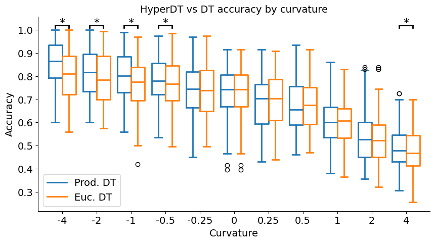
Figure 1: Classification accuracies for Gaussian mixtures on manifolds of varying curvatures using our method (blue) and a CART decision tree (red). The difference in accuracy between the methods becomes more pronounced with higher curvatures, and the methods are identical (not just comparable) at curvature 0. Statistical significance ($p<0.05$) is marked with an asterisk.

In Figure 1, we compare our method to CART in classification accuracy on Gaussian mixtures on a single component manifold $\mathcal{M}$ for both positive and negative curvatures. For each curvature, we tested 100 different samples of 1,000 points in two dimensions with four classes using an 80:20 train-test split. The negative-curvature results extend earlier findings by Chlenski et al. (2024) to the full range of negative curvatures; the positive-curvature results are novel. Both methods perform identically for curvature 0, corroborating the equivalence between our method and CART in the Euclidean case as shown in Appendix C.

4.3 Product manifold benchmarks

In Table 1, we show that our method outperforms Euclidean decision trees in classification accuracies across all tested product manifolds. We follow Gu et al. (2018) in choosing the six signatures tested, but opt to use a Gaussian mixture rather than a graph embedding for our benchmark. For each signature, we tested 20 different samples of 1,000 points with four classes using an 80:20 train-test split. Notably, our method outperformed Euclidean decision trees on all manifolds tested. Comparable random forest results are found in Table 2 in the Appendix.

Table 1: Benchmark results. We report 95% confidence intervals for classification accuracies on mixtures of four Gaussians over a representative sample of product manifolds. Each manifold has 10 total dimensions. Higher scores are bolded; asterisks mark statistical significance ($p<.05$).

Signature	Euc. DT	Prod. DT
$(\mathbb{H}^{5,1})$	$93.6\pm 1.1$	$\mathbf{97.3\pm 0.5^{*}}$
$(\mathbb{S}^{5,1})$	$62.2\pm 1.6$	$\mathbf{64.1\pm 1.5^{*}}$
$\mathbb{H}^{5,1}\times\mathbb{S}^{5,1}$	$93.7\pm 1.1$	$\mathbf{97.3\pm 0.5^{*}}$
$(\mathbb{H}^{2,1})^{5}$	$76.9\pm 1.9$	$\mathbf{78.6\pm 1.9^{*}}$
$(\mathbb{S}^{2,1})^{5}$	$60.4\pm 1.9$	$\mathbf{60.6\pm 1.9}$
$(\mathbb{H}^{2,1})^{2}\times(\mathbb{S}^{2,1})^{2}\times\mathbb{E}^{2}$	$78.2\pm 1.9$	$\mathbf{79.5\pm 1.9^{*}}$

5 Conclusion

Contributions.

We present strong preliminary evidence in favor of mixed-curvature decision tree algorithms. In particular, we motivate and describe our entire algorithm, and demonstrate the effectiveness of our method on effectiveness on component manifolds of all curvatures. We also offer some evidence of our method’s effectiveness for Gaussian mixtures in product spaces.

Future work.

Future work will prioritize more thorough benchmarking of our methods. In particular, we will compare our method to the product space classifier forms described in Skopek et al. (2020) and benchmark node classification on mixed-curvature embeddings for graphs embedded according to the method of Gu et al. (2018). We are especially interested in seeking out high-quality datasets for benchmarking the regression capabilities of our method, as well as in applications to biological data such as spatial transcriptomic.

Other work can include implementing algorithmic improvements such as boosting, exploring the implications of the lack of privileged basis dimensions in non-Euclidean spaces on the performance of decision tree algorithms, implementing other mixed-curvature classifiers such as multinomial and linear regression, testing ensembles of trees individually trained on single component manifolds, and exploring kernel-based interpretations of these methods.

Limitations.

Although this work is still in the early stages of implementation and benchmarking, we believe our method is mature enough to share. However, one limitation of our method is its discontinuity. Although we claim to vary curvature smoothly, the distance functions must change during the transition from negative to zero to positive curvature. Moreover, though the limit of the radius as $K$ approaches $\infty$ is also $\infty$, we lift our Euclidean embeddings to $x_{0}=1$ instead. A continuous unification and thorough benchmarks would substantially improve this work.

Appendix A Gaussian mixture details

A.1 Overall structure

The structure of our sampling algorithm is as follows. Note that, rather than letting $\mathcal{M}$ be a manifold of arbitrary curvature, we force its curvature to be one of $\{-1,0,1\}$ for implementation reasons. This necessitates rescaling steps, which take place in Equations 24, 28, and 34. The result is equivalent to performing the equivalent steps, without rescaling, on a manifold of the proper curvature.

1. Generate $\mathbf{c}$, a vector that divides $m$ samples into $n$ clusters:

   $$\mathbf{p_{raw}} =\langle p_{0},p_{1},\ldots,p_{n-1}\rangle$$ (18)

   $$p_{i} \sim\text{Uniform}(0,1)$$ (19)

   $$\mathbf{p_{norm}} =\frac{\mathbf{p_{raw}}}{\sum_{i=0}^{n-1}p_{i}}$$ (20)

   $$\mathbf{c} =\langle c_{0},c_{1},\ldots c_{m-1}\rangle$$ (21)

   $$c_{i} \sim\text{Categorical}(n,\mathbf{p_{norm}})$$ (22)

2. Sample $\mathbf{M_{euc}}$, an $n\times D$ matrix of $n$ class means:

   $$\mathbf{M_{euc}} =\langle\mathbf{m_{0},m_{1},\ldots,m_{n-1}}\rangle^{T}$$ (23)

   $$\mathbf{m_{i}} \sim\mathcal{N}(0,\sqrt{K}\mathbf{I}).$$ (24)

3. Move $\mathbf{M_{euc}}$ into $T_{0}\mathcal{M}$, the tangent plane at the origin of $\mathcal{M}$, by applying $\psi:\mathbf{x}\to(0,\mathbf{x})$ per-row to $\mathbf{M_{euc}}$:

   $$\mathbf{M_{tan}} =\langle\psi(\mathbf{m_{0}}),\psi(\mathbf{m_{1}}),\ldots\psi(\mathbf{m_{n-1}})\rangle^{T},$$ (25)

   $$\psi:\mathbb{R}^{D} \to\mathbb{R}^{D+1},\ \mathbf{x}\to\langle 0,\mathbf{x}\rangle.$$ (26)

4. Project $\mathbf{M_{tan}}$ onto $\mathcal{M}$ using the exponential map from $T_{0}\mathcal{M}$ to $\mathbf{M_{tan}}$:

   $$\mathbf{M}=\exp_{0}(\mathbf{M_{tan}}).$$ (27)

5. For $0\leq i<n$, sample a corresponding covariance matrix. Here, $\sigma$ is a variance scale parameter than can be set:

   $$\mathbf{\Sigma_{i}}\sim\text{Wishart}(\sigma\sqrt{K}\mathbf{I},D)$$ (28)

6. For $0\leq j<m$, sample $\mathbf{X_{euc}}$, a matrix of $m$ points according to their clusters’ covariance matrices:

   $$\mathbf{X_{euc}} =\langle\mathbf{x_{0},x_{1},\ldots x_{m-1}}\rangle^{T}$$ (29)

   $$x_{j} \sim\mathcal{N}(0,\mathbf{\Sigma_{c_{j}}}).$$ (30)

7. Apply $\psi(\cdot)$ from Eq 26 to each $\mathbf{x_{j}}$ to move it into $T_{0}\mathcal{M}$:

   $$\mathbf{X_{tan}}=\langle\psi(\mathbf{x_{0}}),\psi(\mathbf{x_{1}}),\ldots\psi(\mathbf{x_{m-1}})\rangle^{T}.$$ (31)

8. For each row in $\mathbf{X_{tan}}$, apply parallel transport from $T_{0}\mathcal{M}$ to its class mean:

   $$\mathbf{X_{PT}} =\langle\mathbf{x_{0,\mu},x_{1,\mu},\ldots,x_{m-1,\mu}}\rangle$$ (32)

   $$\mathbf{\mathbf{x}_{j,\mu}} =PT_{0\to\mathbf{m_{c_{j}}}}(\mathbf{x_{j}})$$ (33)

9. Use the exponential map at $T_{\mu}\mathcal{M}$ to move the points onto the manifold:

   $$\mathbf{X}_{\mathcal{M}} =\langle\mathbf{x_{0,\mathcal{M}},x_{1,\mathcal{M}},\ldots,x_{m-1,\mathcal{M}}}\rangle$$ (34)

   $$\mathbf{x_{j,\mathcal{M}}} =\frac{\exp_{\mathbf{m_{c_{j}}}}(\mathbf{x_{j,\mu}})}{\sqrt{K}}$$ (35)

10. Repeat steps 2–9 for as many manifolds as desired; produce a final embedding by concatenating all component embeddings column-wise:

    $$\mathbf{X}=\langle\mathbf{X}_{\mathcal{M}_{0}},\mathbf{X}_{\mathcal{M}_{1}},\ldots\mathbf{X}_{\mathcal{M}_{p}}\rangle$$ (36)

A.2 Equations for manifold operations

First, we provide the forms of the parallel transport operation in hyperbolic, hyperspherical, and Euclidean spaces:

$$PT_{\nu\to\mu}^{\mathbb{H}}(\mathbf{v}) =\mathbf{v}+\frac{\langle\mu-\alpha\nu,\nu\rangle_{\mathcal{L}}}{\alpha+1}(\nu+\mu)$$ (37)

$$\alpha =-\langle\nu,\mu\rangle_{\mathcal{L}}$$ (38)

$$PT_{\nu\to\mu}^{\mathbb{S}}(\mathbf{v}) =\mathbf{v}\cos(d)+\frac{\sin(d)}{d}(\mu-\cos(d)\nu)$$ (39)

$$d =\cos^{-1}(\nu\cdot\mu)$$ (40)

$$PT_{\nu\to\mu}^{\mathbb{E}}(\mathbf{v}) =\mathbf{v}+\mathbf{\mu-\nu}.$$ (41)

The exponential map is defined as follows in each of the three spaces:

$$\exp_{\mu}(\mathbf{u}) =\cosh(\|\mathbf{u}\|_{\mathcal{L}})\mu+\sinh(\|\mathbf{u}\|_{\mathcal{L}})\frac{\mathbf{u}}{\|\mathbf{u}\|_{\mathcal{L}}}$$ (42)

$$\exp_{\mu}(\mathbf{u}) =\cos(\|\mathbf{u}\|)\mu+\sin(\|\mathbf{u}\|)\frac{\mathbf{u}}{\|\mathbf{u}\|}$$ (43)

$$\exp_{\mu}(\mathbf{u}) =\mathbf{u}.$$ (44)

A.3 Relationship to other work

Nagano et al. (2019) developed the overall technique used for a single cluster and a single manifold, i.e. steps 6–9. Chlenski et al. (2024) modified this method to work for mixtures of Gaussians in $\mathbb{H}^{d,1}$, and deployed it for $d\in{2,4,8,16}$. This corresponds to steps 1–5 of our procedure (although note that our covariance matrices are sampled differently in step 5). Thus, our contribution is simply to add step 10, modify step 5 to use the Wishart distribution, and to add curvature-related scaling factors in Equations 24, 28, and 34.

Additionally, to the best of our knowledge we are the first to apply this to hyperspherical manifolds, for which the von Mises-Fisher (VMF) distribution is typically preferred. We do not argue for the superiority of our approach over the VMF distribution in general; however, we prefer to use ours for these benchmarks, as it allows us to draw simpler parallels between manifolds of different curvatures.

Appendix B Product space decision tree pseudocode

Algorithm 1 Product Space Decision Tree

1:  Procedure Fit:

2:      $\mathcal{P}$(signature of) product manifold

3:      $\mathbf{X}$data points

4:      $\mathbf{y}$target labels

5:  Initialize:

6:      $\mathcal{T}$an empty tree

7:  return  $\textsc{FitTree}(\mathbf{X},\mathbf{y},0)$

8:  

9:  Procedure FitTree:

10:      $\mathbf{X}$data points

11:      $\mathbf{y}$target labels

12:      $t$current depth of the tree.

13:  Initialize:

14:      $d_{\text{best}}$dimension of best split,

15:      $\theta_{\text{best}}$angle of best split,

16:      $IG_{\text{best}}$information gain of best split.

17:  for each $d\in\mathbf{D^{\prime}}$ do

18:     $\mathcal{M}\leftarrow$ component manifold for dimension $d$

19:     $\Theta\leftarrow\textsc{GetCandidates}(\mathcal{M},\mathbf{X},d)$

20:     for each candidate $\theta\in\Theta$ do

21:        Partition $\mathbf{X},\mathbf{y}$ into $\mathbf{X^{+},X^{-},y^{+},y^{-}}$ via Eq. 12.

22:        Apply Eq. 10 on $\mathbf{y^{+},y^{-}}$ to compute $IG_{\text{current}}$

23:        if $IG_{\text{current}}>IG_{\text{best}}$ then

24:           $d_{\text{best}},\ \theta_{\text{best}},\ IG_{\text{best}}\leftarrow d,\ \theta,\ IG_{\text{current}}$

25:        end if

26:     end for

27:  end for

28:  if no valid split was found then

29:     return  $\mathcal{N}$, a new leaf node with $\mathbf{y}$ probabilities.

30:  else

31:     Create $\mathcal{N}$, a decision node with $d_{\text{best}}$ and $\theta_{\text{best}}$

32:     $\mathcal{N}_{L}\leftarrow\textsc{FitTree}(\mathbf{X^{-}},\ \mathbf{y^{-}},\ t+1)$

33:     $\mathcal{N}_{R}\leftarrow\textsc{FitTree}(\mathbf{X^{+}},\ \mathbf{y^{+}},\ t+1)$

34:     return  $\mathcal{N}$ with left child $\mathcal{N}_{L}$ and right child $\mathcal{N}_{R}$

35:  end if

36:  

37:  Procedure GetCandidates:

38:      $\mathcal{M}$A component manifold

39:      $\mathbf{X}$A dataset of points in $\mathcal{M}$

40:      $d$A dimension index

41:  if $d$ is the special dimension then

42:     return  empty array []

43:  end if

44:  $\Theta\leftarrow$ Angles of $\mathbf{X}$ via Eq. 11

45:  $\Theta\leftarrow$ sort and deduplicate $\Theta$

46:  return  [$\theta_{m}$ for $\theta_{i},\theta_{i+1}\in\Theta$ via Eq. 14, 15, or 17] (depending on curvature of $\mathcal{M}$).

Appendix C Proof of equivalence for Euclidean case

A classical CART tree splits data points according to whether their value in a given dimension is greater than or less than some threshold value $t$. Midpoints are simple arithmetic means. This can be written as:

$$S^{\prime}(\mathbf{x},d,t) =\begin{cases}1\text{ if }x_{d}>t,\\ 0\text{ otherwise}.\end{cases}$$ (45)

$$m_{DT}(\mathbf{u},\mathbf{v}) =\frac{u_{d}+v_{d}}{2}.$$ (46)

In our transformed decision tree, we lift the data points by applying $\phi:\mathbf{x}\rightarrow(1,\mathbf{x})$ and then check which side of an axis-inclined hyperplane they fall on. The splitting function is based on the angle $\theta$ of inclination with respect to the $(0,d)$ plane, i.e., $\langle 1,x_{d}\rangle$. Our midpoints are computed to ensure equidistance in the original manifold:

$$S(\mathbf{x},d,\theta) =\operatorname{sign}(\sin(\theta)x_{d}-\cos(\theta)x_{0})$$ (47)

$$m_{\mathbb{E}}(\mathbf{u},\mathbf{v}) =\tan^{-1}\left(\frac{2}{u_{d}+v_{d}}\right)$$ (48)

To demonstrate the equivalence of the classical decision tree formulation to our transformed algorithm in $\mathbb{E}$, we will show that Equation 45 is equivalent to Equation 47 and Equation 46 is equivalent to Equation 48 under

$$\theta=\cot^{-1}(t).$$ (49)

C.1 Equivalence of Splits

First, we show that Equations 45 and 47 are equivalent, assuming $t\neq 0$:

$$S(\mathbf{x},d,\theta) =\operatorname{sign}(\sin(\theta)x_{d}-\cos(\theta)x_{0})=1$$ (50)

$$\iff\sin(\theta)x_{d}-\cos(\theta)>0$$ (51)

$$\iff\frac{\sin(\theta)}{\cos(\theta)}x_{d}=\tan(\theta)x_{d}>1$$ (52)

$$\iff x_{d}/t>1$$ (53)

$$\iff x_{d}>t$$ (54)

$$\iff S^{\prime}(\mathbf{x},d,t)=1$$ (55)

C.2 Equivalence of midpoints

Now, we show that Equations 46 and 48 are equivalent:

$$\cot^{-1}(m_{DT}(\mathbf{u},\mathbf{v})) =\cot^{-1}\left(\frac{u_{d}+v_{d}}{2}\right)$$ (56)

$$=\tan^{-1}\left(\frac{2}{u_{d}-v_{d}}\right)$$ (57)

$$=m_{\mathbb{E}}(\mathbf{u},\mathbf{v})$$ (58)

Appendix D Full benchmark table

We report the full version of Table 1 here, in Table 2.

Table 2: Benchmark results with decision trees and random forests. We report 95% confidence intervals for classification accuracies on mixtures of four Gaussians over a representative sample of product manifolds. Each manifold has 10 total dimensions. Higher scores are bolded; asterisks mark statistical significance ($p<.05$).

	Euclidean	Product space	Euclidean	Product space
Signature	decision tree	decision tree	random forest	random forest
$(\mathbb{H}^{5,1})$	$93.6\pm 1.1$	$\mathbf{97.3\pm 0.5^{*}}$	$90.2\pm 3.2$	$\mathbf{97.0\pm 1.4^{*}}$
$(\mathbb{S}^{5,1})$	$62.2\pm 1.6$	$\mathbf{64.1\pm 1.5^{*}}$	$60.3\pm 4.4$	$\mathbf{61.1\pm 4.0}$
$\mathbb{H}^{5,1}\times\mathbb{S}^{5,1}$	$93.7\pm 1.1$	$\mathbf{97.3\pm 0.5^{*}}$	$90.3\pm 2.5$	$\mathbf{97.1\pm 1.4^{*}}$
$(\mathbb{H}^{2,1})^{5}$	$76.9\pm 1.9$	$\mathbf{78.6\pm 1.9^{*}}$	$78.0\pm 4.7$	$\mathbf{80.8\pm 4.2^{*}}$
$(\mathbb{S}^{2,1})^{5}$	$60.4\pm 1.9$	$\mathbf{60.6\pm 1.9}$	$58.2\pm 4.4$	$\mathbf{58.3\pm 4.7}$
$(\mathbb{H}^{2,1})^{2}\times(\mathbb{S}^{2,1})^{2}\times\mathbb{E}^{2}$	$78.2\pm 1.9$	$\mathbf{79.5\pm 1.9^{*}}$	$78.1\pm 4.8$	$\mathbf{81.6\pm 3.9^{*}}$

References

- Breiman (2001) Breiman, L. Random forests. Machine Learning, 45(1):5–32, October 2001. ISSN 1573-0565. doi: 10.1023/A:1010933404324. URL https://doi.org/10.1023/A:1010933404324.
- Breiman (2017) Breiman, L. Classification and Regression Trees. Routledge, New York, October 2017. ISBN 978-1-315-13947-0. doi: 10.1201/9781315139470.
- Chatfield & Collins (1980) Chatfield, C. and Collins, A. J. Introduction to Multivariate Analysis. Springer US, Boston, MA, 1980. ISBN 978-0-412-16030-1 978-1-4899-3184-9. doi: 10.1007/978-1-4899-3184-9. URL http://link.springer.com/10.1007/978-1-4899-3184-9.
- Chlenski et al. (2024) Chlenski, P., Turok, E., Moretti, A., and Pe’er, I. Fast hyperboloid decision tree algorithms, March 2024. URL http://arxiv.org/abs/2310.13841. arXiv:2310.13841 [cs].
- Do Carmo (1992) Do Carmo, M. Riemannian Geometry. Springer US, 1992. URL https://link.springer.com/book/9780817634902.
- Gu et al. (2018) Gu, A., Sala, F., Gunel, B., and Ré, C. Learning Mixed-Curvature Representations in Product Spaces. September 2018. URL https://openreview.net/forum?id=HJxeWnCcF7.
- McNeela et al. (2024) McNeela, D., Sala, F., and Gitter, A. Product Manifold Representations for Learning on Biological Pathways, January 2024. URL http://arxiv.org/abs/2401.15478. arXiv:2401.15478 [cs, q-bio].
- Nagano et al. (2019) Nagano, Y., Yamaguchi, S., Fujita, Y., and Koyama, M. A Wrapped Normal Distribution on Hyperbolic Space for Gradient-Based Learning, May 2019. URL http://arxiv.org/abs/1902.02992. arXiv:1902.02992 [cs, stat].
- Skopek et al. (2020) Skopek, O., Ganea, O.-E., and Bécigneul, G. Mixed-curvature Variational Autoencoders, February 2020. URL http://arxiv.org/abs/1911.08411. arXiv:1911.08411 [cs, stat].
- Wang et al. (2021) Wang, S., Wei, X., Nogueira dos Santos, C. N., Wang, Z., Nallapati, R., Arnold, A., Xiang, B., Yu, P. S., and Cruz, I. F. Mixed-Curvature Multi-Relational Graph Neural Network for Knowledge Graph Completion. In Proceedings of the Web Conference 2021, WWW ’21, pp. 1761–1771, New York, NY, USA, June 2021. Association for Computing Machinery. ISBN 978-1-4503-8312-7. doi: 10.1145/3442381.3450118. URL https://doi.org/10.1145/3442381.3450118.
- Wishart (1928) Wishart, J. The generalised product moment distribution in samples from a normal multivariate population. Biometrika, 20A(1-2):32–52, December 1928. ISSN 0006-3444. doi: 10.1093/biomet/20A.1-2.32. URL https://doi.org/10.1093/biomet/20A.1-2.32.