ON-OFF Neuromorphic ISING Machines using Fowler-Nordheim Annealers

Abstract

We introduce NeuroSA, a neuromorphic architecture specifically designed to ensure asymptotic convergence to the ground state of an Ising problem using an annealing process that is governed by the physics of quantum mechanical tunneling using Fowler-Nordheim (FN). The core component of NeuroSA consists of a pair of asynchronous ON-OFF neurons, which effectively map classical simulated annealing (SA) dynamics onto a network of integrate-and-fire (IF) neurons. The threshold of each ON-OFF neuron pair is adaptively adjusted by an FN annealer which replicates the optimal escape mechanism and convergence of SA, particularly at low temperatures. To validate the effectiveness of our neuromorphic Ising machine, we systematically solved various benchmark MAX-CUT combinatorial optimization problems. Across multiple runs, NeuroSA consistently generates solutions that approach the state-of-the-art level with high accuracy (greater than 99%), and without any graph-specific hyperparameter tuning. For practical illustration, we present results from an implementation of NeuroSA on the SpiNNaker2 platform, highlighting the feasibility of mapping our proposed architecture onto a standard neuromorphic accelerator platform.

1 Introduction

Quadratic Unconstrained Binary Optimization (QUBO) and Ising models are considered fundamental to solving many combinatorial optimization problems (COP) [1, 2, 3] and in literature, both classical and quantum hardware accelerators have been proposed to efficiently solve QUBO/Ising problems [4, 5]. These accelerators use some form of annealing to guide the collective dynamics of the underlying optimization variables (e.g. spins) toward the global optima of the COP, which correspond to a specific system’s ground energy states. Examples of such accelerators include superconducting qubits-based quantum annealers [6], optical circuits-based coherent Ising machines (CIM) on [7, 8], CMOS-based oscillator networks [9, 10], memristor-based Hopfield Network [11, 12, 13], and digital circuits-based simulated annealing (SA) [14, 15, 16, 17]. Quantum Ising machines that use quantum annealing can theoretically guarantee finding the optimal solution to the QUBO/Ising problem, however, the approach cannot yet be physically scaled to solve large-scale problems [18, 19, 20, 21]. On the other hand, classical QUBO/Ising solvers such as simulated bifurcation machine (SBM) [22] and memristor-based Hopfield Network [11], exploit non-linear oscillator dynamics and noise injection to explore the solution space. Memristor-based Ising machines have been reported to achieve high energy efficiency, however, these platforms have only been demonstrated for small-scale or general purpose COPs [12].

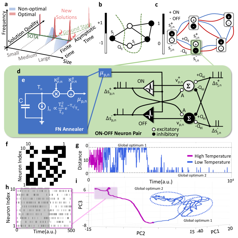
Figure 1: NeuroSA motivation for mapping of optimal simulated annealing into a neuromorphic architecture: (a) For larger/more complex COPs NeuroSA produces distribution of solutions that is concentrated near the SOTA and has the potential to produce novel, previously unknown solution that is closer to the Ising ground state; A MAX-CUT problem defined over a (b) graph with weights $Q_{ij}$ which is decomposed into (c) pairs of ON-OFF neurons by NeuroSA. (d) Each ON-OFF integrate-and-fire neurons are coupled to each other by an excitatory synapse with weight $A$ and the pair is connected differentially to other ON-OFF neuron pairs through the synaptic weights $Q_{ij},-Q_{ij}$. The thresholds for both ON-OFF neurons are dynamically adjusted by an (e) FN annealer which comprises an FN integrator, an exponentially-distributed noise source $\mathcal{N}_{n}^{E}$ and a Bernoulli noise source $\mathcal{N}_{n}^{B}$; Illustration of NeuroSA dynamics for a MAX-CUT graph with 10 vertices connected by a weight matrix $\mathbf{Q}$ shown in (f); (g) Evolution of the distance between the solutions generated by NeuroSA to the two known ground state solutions at a given time-instant which highlights the escape mechanisms in the high- and low-temperature regimes; (h) Raster plot of aggregated spiking activity generated by the ON and OFF neuron pairs, and (i) visualization of the NeuroSA trapping and escape dynamics using a PCA-based projection of the network spiking activity estimated within a moving time-window.

Neuromorphic hardware accelerators as a platform for solving large-scale Ising problems: Advances in neuromorphic hardware have now reached a point where the platform can simulate networks comprising billions of spiking neurons and trillions of synapses. Implementation of these neuromorphic supercomputers range from commercial-off-the-shelf (COTS) CPU-, GPU-based platforms [23, 24] to custom FPGA-, multi-core-, ASIC-based platforms [25, 26, 27]. As an example, the SpiNNaker2 microchip  [28], which has been used for illustrative experiments in this paper, can integrate more than 152,000 programmable neurons with more than 152 million synapses in total. While the primary motivation for developing these platforms has been to emulate/study neurobiological functions [29, 30] and to implement artificial intelligence (AI) tasks [31, 32, 33] with much needed energy efficiency  [34], it has been argued that the neuromorphic advantage can be demonstrated for tasks that can exploit noise and non-linear dynamics inherent in the current neuromorphic systems. These approaches exploit the emergent properties of an energy or entropy minimization process [35, 36], phase transition and criticality [37], chaos [38], and stochasticity [39, 40, 41], both at the level of an individual neuron [42, 43, 22] and at the system level such as the Hopfield Network [35, 11] and Boltzmann Machines [44, 45]. Recently, neuromorphic advantage in energy efficiency has been demonstrated recently for solving optimization problems [32, 46] and for simulating stochastic systems like random walks [47]. These specific implementations exploit the high degree of parallelism inherent in neuromorphic architectures for efficient Monte Carlo sampling, and for implementing Markov processes both of which are important for solving Ising problems. Previous attempts to solve Ising problems using neuromorphic hardware [13, 12] have been limited to small networks with no guarantee on the quality of the solution if the problem size or complexity is increased. This is highlighted in Fig. 1(a), which plots the distribution of the quality of the solutions obtained across independent runs of an Ising machine. When the problem size is small, distributions obtained by different Ising machines are concentrated around the state-of-the-art (SOTA) solution, which typically coincides with or is close to the Ising ground state. However, as the problem size/complexity increases, finding the Ising ground state becomes more difficult, and a non-optimal machine will produce a distribution of solutions with heavy tails, as shown in Fig. 1(a). These Ising machines would require multiple runs and extensive hyper-parameter tuning, and hence a long wait time to obtain state-of-the-art (SOTA) solutions. Also, for large-scale COP for which the SOTA might not be known apriori, only loose bounds on the quality of the solution can be estimated [48]. Simulated annealing (SA) algorithms, on the other hand, can provide asymptotic guarantees of finding the QUBO/Ising ground state provided the annealing schedule follows a specific dynamics [49, 50, 51]. Hence, a neuromorphic architecture that is functionally isomorphic to the SA algorithm with an optimal annealing schedule should produce high-quality solutions across different runs. This feature is highlighted in Fig. 1a by the desired (or optimal) distribution that is concentrated near the SOTA. Furthermore, as shown in Fig. 1a, having an asymptotic optimality guarantee will also ensure that a long run-time might produce at least a solution that is better than the current SOTA, if the current SOTA is not already the ground state of the COP. In this regard, a neuromorphic supercomputer could rely on hardware acceleration to possibly search for or discover previously unknown solutions.

How can optimal simulated annealing algorithms be mapped onto large-scale neuromorphic architectures? The key underpinnings of any neuromorphic architecture are: (a) asynchronous (or Poisson) dynamics that are generated by a network of spiking neurons; and (b) efficient and parallel routing of spikes/events between neurons across large networks. Both these features are essential for solving the Ising problem and efficient mapping of SA onto neuromorphic architecture. In its general form Ising problem minimizes a function (or a Hamiltonian) $H(\mathbf{s})$ of the spin state vector $\mathbf{s}$ according to

$$\min_{\mathbf{s}\in\{-1,+1\}^{D}}H(\mathbf{s})=\frac{1}{2}\mathbf{s}^{\intercal}\mathbf{Q}\mathbf{s}+\mathbf{b}^{T}\mathbf{s}$$ (1)

where $\mathbf{b}\in\mathbb{R}^{D}$ represents an external field or bias vector and can also be used to introduce additional constraints into the Ising problem [52]. Without sacrificing generality, our focus can be narrowed down to problems where $\mathbf{b}=\mathbf{0}$ in which case Ising problems become equivalent to MAX-CUT problems (shown in SI S1.2 and S1.1). For a simple MAX-CUT graph depicted in Fig. 1b, each of the spin variables, denoted as $s_{i}\in\{-1,+1\}$, where $i=1,..,D$, is associated with one of the $D$ vertices in the graph $\mathcal{G}$. The graph’s edges are represented by a matrix $\mathbf{Q}\in\mathbb{R}^{D\times D}$, wherein $Q_{ij}$ signifies the weight associated with the edge connecting vertices $i$ and $j$. Given the graph $\mathcal{G}$, the objective of the MAX-CUT problem is to partition the vertices into two classes, maximizing the number of edges between them. If an ideal asynchronous operation is assumed (see Methods section 3.1), then at any time instant $n$, only one spin (say the $p^{th}$ spin) changes its state by $\Delta\mathbf{s}_{p,n}\in\{-1,0,+1\}$. In this case, the function $H$ decreases or $\Delta H_{n}<0$, if and only if the condition

$$\Delta s_{p,n}\left[\sum_{j=1}^{D}Q_{pj}s_{j,n-1}\right]<0$$ (2)

is satisfied. The inherent parallelism of neuromorphic hardware ensures that the pseudo-gradient $\sum_{j=1}^{D}Q_{pj}s_{j,n-1}$ is computed at a rate faster than the rate at which events $\Delta s_{p,n}$ are generated. The condition described in Eq. 2, when combined with the simulated annealing’s probabilistic acceptance criterion [49], leads to a neuromorphic mapping based on coupled ON-OFF integrate-and-fire neurons where the $p^{th}$ ON-OFF pair is shown in Fig. 1d. Please refer to the Methods section 3 for the derivation of the ON-OFF neuron model. The $p^{th}$ ON-OFF neuron pair is differentially connected to the $j^{th}$ neuron pair through the synaptic weights $Q_{pj},-Q_{pj}$. The spikes generated by this $p^{th}$ post-synaptic ON-OFF neuron pair $\Delta s_{p,n}^{+},\Delta s_{p,n}^{-}\in\{0,1\}$ differentially encodes the change in the $p^{th}$ spin state, and the cumulative state $s_{j,n}$ of the pre-synaptic neuron is estimated by continuously integrating the input spikes $\Delta s_{j,n}^{+},\Delta s_{j,n}^{-}$ received from the $j^{th}$ neuron. To ensure that the spiking activity of the ON-OFF neuronal network is functionally isomorphic to the acceptance/rejection dynamics of an SA algorithm, the firing threshold $\mu_{p,n}$ of the $p^{th}$ neuron adjusted over time by a Fowler-Nordheim (FN) annealer, shown in Fig. 1d.

A Fowler-Nordheim dynamical system can produce dynamic thresholds that correspond to the optimal annealing schedule: One of the key results from the SA literature [50, 51] is the proposition that a temperature cooling schedule that follows $\sim\frac{c}{\log(1+n)}$ can guarantee asymptotic convergence to the QUBO/Ising ground state, where $c$ denotes the largest depth of any local minimum of Ising Hamiltonian $H(\mathbf{s})$. A dynamical systems model in Fig. 1e comprising of a time-varying Fowler-Nordheim (FN) current element $J_{n}$ [53] can generate the optimal $T_{n}=\frac{T_{0}}{\log(1+n/C)}$ according to [54], where $T_{0}$ and $C$ are Fowler-Nordheim annealing hyperparameters (see Methods section 3.3). The FN dynamics can then be combined with the independent identically distributed (i.i.d) random variables $\mathcal{N}_{p,n}^{E}$ and $\mathcal{N}_{p,n}^{B}$ to determine the dynamic firing threshold $\mu_{n,p}$ for each ON-OFF integrate-and-fire neuron pair $p$. $\mathcal{N}_{p,n}^{E}$ is drawn from an exponential distribution where as $\mathcal{N}_{p,n}^{B}$ is drawn from a Bernoulli distribution with values $\{0,1\}$. The choice of the two distributions ensures that every neuron has a finite probability of firing, which is equivalent to satisfying the irreducibility and aperiodicity conditions in SA.

The ON-OFF neuron pair and the integrated FN annealer, shown in Fig. 1c form the basic computational unit of NeuroSA which can be used to solve Ising problems on different neuromorphic hardware platforms. Due to the functional isomorphism between NeuroSA and the optimal SA algorithm, the hardware to accelerate and asymptotically approach the Ising ground state, as highlighted in Fig. 1a. We show in the results that even when NeuroSA is run for a finite duration, the machine produces the distribution of solutions that is concentrated around the SOTA, as shown in Fig. 1a, and this is achieved without significant tuning of hyperparameters.

2 Results

The performance of NeuroSA is evaluated for MAX-CUT graphs for which the ground state can either be determined by brute-force search or for which the SOTA is well documented in literature [55, 22]. Note that even though we have chosen MAX-CUT problems as a benchmark, the Ising model is general enough and can be used for solving other COPs [56].

2.1 Experiments using small-scale graphs

NeuroSA is first applied to a 10-node MAX-CUT graph described by the interconnection matrix $\mathbf{Q}$ shown in Fig. 1f. For this graph, the two degenerate ground states exist (due to the gauge symmetry where $\mathbf{s}\leftrightarrow-\mathbf{s}$) and can be found by an exhaustive search over all possible spin state configurations. In Fig. 1g we plot the Hamming distance between the solution found by NeuroSA at a time instant from the two global optima. It is evident from Fig. 1g that, like SA, the dynamics of NeuroSA can be categorized into two phases: the high-temperature regime and the low-temperature regime. These regimes are determined by the firing threshold $\mu(t)$ in Fig. 1c. To visualize the network dynamics, the aggregated spiking rate for each of the ON-OFF neuron pairs is calculated using a moving window as shown in Fig. 1h and is projected onto a reduced $3$-D space spanned by its three most dominant principal component vectors, as shown in Fig. 1i. This PCA based approach is a standard practice in analyzing spiking data [57] and details of the approach are described in Methods section 3.5. In the high-temperature phase, the network dynamics evolve along the network gradient, resulting in faster convergence along a smooth trajectory as depicted in Fig. 1i. As the temperature cools down, NeuroSA exploration is trapped in the neighborhood of one of the two global optima, as depicted in Fig. 1g and i. In the neighborhood, the dynamics follow a random walk, however, the dynamics can periodically escape one of the global optima for further exploration and possibly converge to the second global optimum. This is highlighted in Fig. 1i by the continuous trajectory connecting the two optima/attractors. Eventually, as shown in Fig. 1g, due to the annealing process the dwell-time of dynamics in the neighborhood of the optima increases with time. Note that state-space exploration in the low-temperature regime is a significant problem in SA algorithms and literature hybrid quantum-classical methods [58] have been proposed to accelerate this process. In NeuroSA, the Fowler-Nordheim dynamical process allows for a finite probability of escape even in the low-temperature regime; however, this probability diminishes over time.

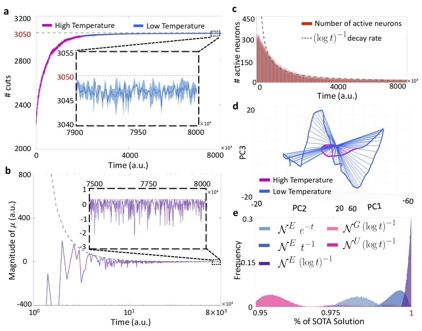
Figure 2: NeuroSA dynamics for the $G15$ MAX-CUT graph with 800 vertices and 4661 edges: (a) convergence plot showing steady increase in the solution quality with the inset showing fluctuations near $3050$ cuts which is the current SOTA for this graph; (b) dynamics of the firing threshold with inset showing sparse but large fluctuations that trigger escape mechanisms; (c) plot showing the number of active neurons decaying following $\sim\frac{1}{\log t}$ without the contribution of the Bernoulli r.v. $\mathcal{N}^{B}$; (d) PCA trajectory of the NeuroSA dynamics where the initial (high temperature) regime follows a path defined by the network gradient and the trajectory near convergence (or low-temperature path) exhibits expanding exploration of the solution space; and (e) distribution of the $G15$ solutions obtained for different annealing schedules ($e^{-t},(\log t)^{-1},t^{-1}$) and noise statistics (exponential - denoted by $\mathcal{N}^{E}$, Gaussian - denoted by $\mathcal{N}^{G}$ and Uniform - denoted by $\mathcal{N}^{U}$)

2.2 Experiments using medium-scale graph

We next apply NeuroSA for a MAX-CUT problem to a graph where the ground state is not known, but the SOTA solution is well documented. We chose the G$15$, a $800$-node, binary weighted, planar graph [59] for which the SOTA is $3050$ cuts [22]. NeuroSA architecture was simulated on a CPU-based platform and the hardware mapping procedure is described in the Methods section 3.4 and the pseudo-code for the implementation is presented in the Supplementary section S1.3.

The dynamics of the noisy firing threshold $\mu_{n}$ is shown in Fig. 2b and is bounded by $T_{n}\sim\frac{1}{\log(n)}$ (depicted in the figure as the dotted line), produced by the FN annealer. As the envelope of the threshold decreases it inhibits the probability of neurons to fire as is shown by the histogram in Fig. 2c. During the initial phases of the convergence, there is a gap between the $\frac{1}{\log(n)}$ envelope and the number of active neurons (or the neurons whose membrane potential exceeds the firing threshold). Thus, in this phase the dynamics of the network seems to be governed by the network gradient. However, the tails of the histogram fits the $\frac{1}{\log(n)}$ reasonably well, highlighting the influence of the FN-based escape mechanism on the network dynamics. The network population dynamics is depicted by the PCA trajectory of the aggregated spiking rate and is plotted in Fig. 2d. Similar to the results for the small-scale graph in Fig. 1i, the trajectory reflects the evolution of the NeuroSA system as it explores the solution space. The exploration in the high temperature regime follows a more confined trajectory in the PCA space, indicating that the network dynamics evolve in the direction of the Ising energy gradient. As the temperature cools down near convergence, the NeuroSA dynamics are dominated by the random-walk and sporadic escape mechanisms with no specific direction, as shown in Fig. 2d.

Fig. 2e plots the distribution of the solution quality (normalized with respect to SOTA) when different cooling schedules are chosen and the r.v. $N^{E}$ are chosen from different statistical distributions. In particular, previous neuromorphic Ising models and stochastic models have used Gaussian noise as a mechanism for asymptotic exploration and for escaping local minima. However, the results in Fig. 2e show that this approach produces distributions with longer tails and in some cases solutions that are significantly worse than the SOTA. Only for a FN annealer and with an exponentially distributed noise $N^{E}$, the distribution of solutions obtained by NeuroSA are more concentrated around the SOTA.

2.3 Benchmarking NeuroSA for different MAX-CUT graphs

Next the NeuroSA architecture was benchmarked for solving MAX-CUT problems on different Gset graphs. Fig. 3 provides a detailed evaluation of the NeuroSA algorithm’s performance on the Gset benchmarks, with results generated using both traditional CPU (software) and the SpiNNaker2 platform. The architecture is configured similarly for both hardware platforms and across all benchmark tests. This uniformity is important, as it demonstrates that NeuroSA’s performance is robust across and agnostic to different MAX-CUT graph complexities. Also, it obviates painstaking hyperparameter tuning for each set of graphs or problems.

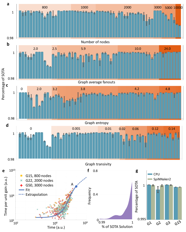
Figure 3: Sweep of NeuroSA on Gset benchmarks with uniform simulation time and hyperparameter configuration. (a)-(d) plot the solution obtained by NeuroSA in both CPU ($10^{8}$ iterations) and SpiNNaker2 as percentages of the SOTA solution reported in [55]. Different metrics that characterize the complexity of the corresponding Gset problem are used for ordering the solution, with the darker region corresponding to higher complexity in the particular measure: (a) the number of vertices in the graph; (b) the average fan-out of each node; (c) the graph entropy; (d) the graph transitivity. (e) Plots the instantaneous time per unit gain in solution for $3$ different Gset benchmarks. A super-exponentially increasing trend is fitted and extrapolated. (f) Plots the distribution of all obtained solutions across $4$ sweeps on all benchmark problems, showing that the consistency of NeuroSA architecture is resilient to simulation time and model hyperparameter. (g) Solution obtained from NeuroSA implementation on the SpiNNaker2 platform.

Fig. 3a-d report the obtained solution by NeuroSA architecture on a CPU platform normalized with respect to the known SOTA solution for a particular MAX-CUT graph [55, 22]. Also, shown in Fig. 3a-d are error bars that correspond to the maximum and the minimum values obtained across 5 runs. As evident from the figures, the NeuroSA solutions consistently reach within $99\%$ of the SOTA for nearly all Gset benchmarks and for every run, with $\sim 50\%$ of the runs achieving the SOTA solution. For this experiment, only one set of hyperparameters $T_{0},\mathcal{N}^{E},C$ was chosen for all Gset benchmarks. This could be one reason for the variance to differ slightly across different MAX-CUT problems which vary in their complexity. Determining the complexity of the different combinatorial problems is a difficult task in itself. Therefore, to gain more insight, the simulation results are methodically organized based on various common graph complexity metrics. Fig. 3a organizes the graphs by the graph size, namely the number of vertices; Fig. 3b organizes the graphs by the average fan-out per node; Fig. 3c sorts them by graph entropy, measuring the randomness in connectivity [60]; Fig. 3d adopts network transitivity, focusing on node connectivity density, indicating clustering within the network [61]. The average fan-out per node measures the typical number of direct connections (outgoing edges) each node has, providing a basic indication of the graph’s overall connectivity and potential for information spread. Graph entropy, on the other hand, quantifies the randomness or disorder in the graph by analyzing the distribution of these connections across all nodes. It offers insights into how evenly or unevenly the connections are distributed, with higher entropy indicating a more complex or disordered network structure. The global clustering coefficient, also known as transitivity, measures the degree to which nodes in a graph tend to cluster together. This coefficient assesses the overall tendency of nodes to create tightly knit groups, with higher values suggesting a greater prevalence of interconnected triples of nodes, which can indicate a robust local structure within the network. While the average fan-out per node provides a simple measure of connectivity, it does not capture the nuances of how these connections are configured, which is where graph entropy and the global clustering coefficient come into play. Graph entropy complements the average fan-out by assessing the variability in node connectivity, highlighting potential inequalities or irregularities in how nodes are linked. In contrast, the global clustering coefficient focuses on the tendency to form local groups, offering a view of the graph’s compactness and the likelihood of forming tightly connected communities. Together, these metrics provide a multi-dimensional view of a graph’s complexity, indicating not only how many connections exist, but also how they are organized and how they foster community structure and network resilience. The results shown in Fig. 3a- 3d demonstrate that NeuroSA can find high-quality solutions irrespective of the complexity of the graph. Note that all these experiments were conducted with only a choice of hyperparameters which obviates the need for fine-tuning and repeated runs.

Fig. 3e presents an analysis of the time required per unit gain in the solution for three distinct Gset benchmarks. The plots reveal an increasing cost (computational time) to achieve marginal improvement in the quality of the solution. The key metric in the plot Fig. 3e is the ratio between the time needed to obtain a unit improvement to the total run time. As it becomes harder to find better solutions, the ratio tends to unity (as shown by the extrapolation curve and the transition point $A$) which might highlight the point of diminishing returns. This could be taken as a hardware-agnostic stopping criterion for a COP. The robustness of the NeuroSA architecture on different Gset problems is illustrated in Fig. 3f, which plots the distribution of all solutions obtained across multiple sweeps, showcasing that with consistent settings, NeuroSA maintains stable performance regardless of the graph’s complexity. This uniform application of the NeuroSA algorithm highlights its potential as a universal solver that can be effectively applied across a wide range of problem settings without requiring adjustments to its core configuration or the underlying hyperparameters. However, the absolute run-time can be significantly reduced by using dedicated neuromorphic accelerators like SpiNNaker2. Fig. 3g shows the results when NeuroSA is implemented on the SpiNNaker2 platform (details provided in SI S1.4) for some of the Gset benchmarks. The results show similar or better solutions than the CPU/software implementation of NeuroSA which highlights the importance of hardware acceleration.

3 Materials and Methods

3.1 Asynchronous Ising Machine Model

QUBO and Ising formulations are interchangeable through a variable transform $s\leftrightarrow\frac{1+s}{2}$, and hence, without any loss of generality, we consider the following optimization problem

$$\min_{\mathbf{s}\in\{-1,+1\}^{D}}H(\mathbf{s})=\frac{1}{2}\mathbf{s}^{\intercal}\mathbf{Q}\mathbf{s}$$ (3)

where $\mathbf{s}=\left[s_{1},s_{2},..,s_{D}\right]$ denotes a spin vector comprising of binary optimization variables. Because $s_{j}^{2}=1,\forall j=1...D$, Eq. 3 is equivalent to

$$\min_{\mathbf{s}\in\{-1,+1\}^{D}}H(\mathbf{s})=\frac{1}{2}\mathbf{s}^{\intercal}\mathbf{Q}\mathbf{s}\quad\text{with }Q_{ii}=0$$ (4)

Note the matrix $\mathbf{Q}$ can be symmetrized by $\mathbf{Q}\leftarrow\frac{1}{2}(\mathbf{Q}+\mathbf{Q}^{\intercal})$ without changing the solution to Eq. 3. Let the vector $\mathbf{s}$ at time instant $n$ be denoted by $\mathbf{s}_{n}$ and the change in $\mathbf{s}$ be denoted as $\Delta\mathbf{s}_{n}$, then

$$\Delta H_{n}=H(\mathbf{s}_{n-1}+2\Delta\mathbf{s}_{n})-H(\mathbf{s}_{n-1}),$$ (5)

where $\Delta\mathbf{s}_{n}=\{-1,0,+1\}^{D}$ and $\Delta s_{j,n}s_{j,n-1}=-1,0,\forall j=1...D$ ensures that the spin either flips or remains unchanged. Then,

$$\Delta H_{n}=\Delta\mathbf{s}_{n}^{\intercal}\mathbf{Q}(\mathbf{s}_{n-1}+2\Delta\mathbf{s}_{n})+\mathbf{s}_{n-1}^{\intercal}\mathbf{Q}\Delta\mathbf{s}_{n}$$ (6)

Using $Q_{ij}=Q_{ji}$,

$$\Delta H_{n}=2\Delta\mathbf{s}_{n}^{\intercal}\mathbf{Q}(\mathbf{s}_{n-1}+\Delta\mathbf{s}_{n})$$ (7)

and applying $s_{p,n-1}\Delta s_{p,n}=-1,\forall n,p$ leads to

$$\Delta H_{n}=2\sum_{p\in\mathcal{C}}\Delta s_{p,n}\left[\sum_{j\notin\mathcal{C}}Q_{pj}s_{j,n}\right],$$ (8)

where the set $\mathcal{C}=\{i:\Delta s_{i,n}\not=0\}$ denotes the neurons that do not fire at time-instant $n$. Solving Eq. 3 involves solving the sequentially sub-problem: $\forall n$, find $\Delta s_{p,n}\in\{-1,0,+1\}^{D}$ such that $\sum_{p\in\mathcal{C}}\Delta s_{p,n}\left[\sum_{p\notin\mathcal{C}}Q_{pj}s_{j,n}\right]<0$, which in itself is a combinatorial problem. By adopting asynchronous firing dynamics, the problem of searching for the set of firing neurons can be simplified. For an asynchronous spiking network, only one of the neurons can emit a spike at any time instant $n$ (due to Poisson statistics), which leads to

$$\Delta H_{n}=2\Delta s_{p,n}\left[\sum_{j=1}^{D}Q_{pj}s_{j,n-1}\right]$$ (9)

where we have used $Q_{pp}=0$. Hence, $\Delta H_{n}<0$, if and only if

$$\Delta s_{p,n}\left[\sum_{j=1}^{D}Q_{pj}s_{j,n-1}\right]<0.$$ (10)

3.2 Derivation of NeuroSA’s neuron model

In its most general form [49], a simulated annealing algorithm solves Eq. 3 by accepting or rejecting choices of $\Delta s_{p,n}$ according to

$$\text{Accept}\quad\Delta s_{p,n}:\text{if}\quad B\exp\left(\frac{-\Delta H_{n}}{T_{n}}\right)>u_{n},$$ (11)

where $u_{n}$ is a uniformly distributed r.v. between $\left[0,1\right]$, and $B>1$ is a hyper-parameter, $T_{n}>0$ denotes the temperature at time-instant $n$. Eq. 11 is equivalent to

$$\text{Accept}\quad\Delta s_{p,n}:\text{if}\quad\Delta H_{n}<-T_{n}\log\left(\frac{u_{n}}{B}+\epsilon\right)$$ (12)

or

$$\Delta s_{p,n}\left[\sum_{j=1}^{D}Q_{pj}s_{j,n-1}\right]<-T_{n}\mathcal{N}_{n}^{E}$$ (13)

where $\mathcal{N}_{n}^{E}=\log\left(\frac{u_{n}}{B}+\epsilon\right)$ is an exponentially distributed r.v. We have introduced a small additive term $\epsilon>0$ to ensure numerical stability when drawing samples with values close to zero. In practice, $\epsilon$ is determined by the precision of the hardware platform and hence will be considered a hyperparameter for NeuroSA. Eq. 13 can be written case-by-case as

$$\Delta s_{p,n}=\left\{\begin{array}[]{ c l }+1&\quad\textrm{if }s_{p,n-1}=-1\textrm{ and }-\sum_{j=1}^{D}Q_{pj}s_{j,n-1}>T_{n}\mathcal{N}_{n}^{E}\\ -1&\quad\textrm{if }s_{p,n-1}=+1\textrm{ and }\sum_{j=1}^{D}Q_{pj}s_{j,n-1}>T_{n}\mathcal{N}_{n}^{E}\\ 0&\quad\textrm{otherwise}\end{array}\right.$$ (14)

Decomposing the variables differentially as $\Delta s_{p,n}=\Delta s_{p,n}^{+}-\Delta s_{p,n}^{-}$, $s_{p,n}=s_{p,n}^{+}-s_{p,n}^{-}$, $\Delta s_{p,n}^{+}$, $\Delta s_{p,n}^{-}$, $s_{p,n}^{+}$, $s_{p,n}^{-}>0$ leads to $s_{p,n}^{+}=\sum_{k=1}^{n}\left[\Delta s_{p,k}^{+}-\Delta s_{p,k}^{-}\right]$, $s_{p,n}^{-}=\sum_{k=1}^{n}\left[-\Delta s_{p,k}^{+}+\Delta s_{p,k}^{-}\right]$. Eq. 14 is therefore equivalent to

$$\Delta s_{p,n}^{+}=\left\{\begin{array}[]{ c l }1&\quad\textrm{if }s_{p,n-1}^{+}=0\textrm{ and }\displaystyle\sum_{k=1}^{n-1}\displaystyle\sum_{j=1}^{D}Q_{pj}\left[-\Delta s_{p,k}^{+}+\Delta s_{p,k}^{-}\right]>T_{n}\mathcal{N}_{n}^{E}\\ 0&\quad\textrm{otherwise}\end{array}\right.$$ (15)

which corresponds to the spiking criterion for an ON neuron and

$$\Delta s_{p,n}^{-}=\left\{\begin{array}[]{ c l }1&\quad\textrm{if }s_{p,n-1}^{-}=0\textrm{ and }\displaystyle\sum_{k=1}^{n-1}\displaystyle\sum_{j=1}^{D}Q_{pj}\left[\Delta s_{p,k}^{+}-\Delta s_{p,k}^{-}\right]>T_{n}\mathcal{N}_{n}^{E}\\ 0&\quad\textrm{otherwise}\end{array}\right.$$ (16)

which corresponds to the spiking criterion for an OFF neuron. Introducing a RESET parameter $A\gg|T_{n}\log\left(\frac{u_{n}}{B}+\epsilon\right)|$, Eq. 15 and 16 are equivalent to the ON neuron model

$$\Delta s_{p,n}^{+}=\left\{\begin{array}[]{ c l }1&\quad\textrm{if }v_{p,n}^{+}>T_{n}\mathcal{N}_{n}^{E},\\ &\quad\textrm{where}\quad v_{p,n}^{+}=v_{p,n-1}^{+}+\sum_{j=1}^{D}Q_{pj}(\Delta s_{j,n-1}^{-}-\Delta s_{j,n-1}^{+})\\ &\quad\quad\quad\quad\quad+A\Delta s_{p,n-1}^{-}-A\Delta s_{p,n-1}^{+}\\ 0&\quad\textrm{otherwise}\end{array}\right.$$ (17)

and the OFF neuron model

$$\Delta s_{p,n}^{-}=\left\{\begin{array}[]{ c l }1&\quad\textrm{if }v_{p,n}^{-}>T_{n}\mathcal{N}_{n}^{E},\\ &\quad\textrm{where}\quad v_{p,n}^{+}=v_{p,n-1}^{+}+\sum_{j=1}^{D}Q_{pj}(\Delta s_{j,n-1}^{+}-\Delta s_{j,n-1}^{-})\\ &\quad\quad\quad\quad\quad+A\Delta s_{p,n-1}^{+}-A\Delta s_{p,n-1}^{-}\\ 0&\quad\textrm{otherwise}\end{array}\right.$$ (18)

The variables $v_{p,n}^{+},v_{p,n}^{-}$ represent the membrane potentials of the ON-OFF integrate-and-fire neurons at the time instant $n$. To ensure that all neurons are equally likely to be selected (to satisfy the ergodicity property of SA), we introduce a Bernoulli r.v. for every neuron $p$ as

$$\mathcal{N}_{p}^{B}=\left\{\begin{array}[]{ c l }1&\quad\textrm{with probability }1-\eta\\ 0&\quad\textrm{with probability }\eta\end{array}\right.$$ (19)

which leads to the ON neuron model

$$\Delta s_{p,n}^{+}=\left\{\begin{array}[]{ c l }1&\quad\textrm{if }v_{p,n}^{+}>\mu_{p,n},\\ 0&\quad\textrm{otherwise}\end{array}\right.$$ (20)

and the OFF neuron model

$$\Delta s_{p,n}^{-}=\left\{\begin{array}[]{ c l }1&\quad\textrm{if }v_{p,n}^{-}>\mu_{p,n},\\ 0&\quad\textrm{otherwise,}\end{array}\right.$$ (21)

where $\mu_{n,p}=T_{n}\mathcal{N}_{n}^{E}+A\mathcal{N}_{p,n}^{B}$ denotes the shared noisy threshold between the $p^{th}$ pair of ON-OFF neurons at time instance $n$. The ON-OFF construction ensures that $\Delta s_{p,n}^{+}\Delta s_{p,n}^{-}=0,\forall p,n$, which leads to the following fundamental ON-OFF integrate-and-fire neuron model of NeuroSA which is summarized as: The ON-OFF neuron’s membrane potentials $v_{p,n}^{+},v_{p,n}^{-}\in\mathbb{R}$ evolve as

$$v_{p,n}^{+}\leftarrow v_{p,n-1}^{+}+\sum_{j=1}^{D}Q_{pj}(\Delta s_{j,n-1}^{-}-\Delta s_{j,n-1}^{+})+A\Delta s_{p,n-1}^{-}$$ (22)

$$v_{p,n}^{-}\leftarrow v_{p,n-1}^{-}+\sum_{j=1}^{D}Q_{pj}(\Delta s_{j,n-1}^{+}-\Delta s_{j,n-1}^{-})+A\Delta s_{p,n-1}^{+}$$ (23)

where $A>0$ is a constant that represents an excitatory synaptic coupling between the ON and the OFF neurons, as shown in Fig. 1d. The ON and OFF neurons generate a spike when their respective membrane potential exceeds a time-varying noisy threshold $\mu_{p,n}$ according to

$$\Delta s_{p,n}^{+}=\left\{\begin{array}[]{ c l }1&\quad\textrm{if }v_{p,n}^{+}>T_{n}\mathcal{N}_{p,n}^{E}+A\mathcal{N}_{p,n}^{B},\\ 0&\quad\textrm{otherwise}\end{array}\right.$$ (24)

and

$$\Delta s_{p,n}^{-}=\left\{\begin{array}[]{ c l }1&\quad\textrm{if }v_{p,n}^{-}>T_{n}\mathcal{N}_{p,n}^{E}+A\mathcal{N}_{p,n}^{B},\\ 0&\quad\textrm{otherwise}\end{array}\right.$$ (25)

after which the membrane potentials are RESET by subtraction according to

$$v_{p,n}^{+}\leftarrow v_{p,n}^{+}-A\Delta s_{p,n}^{+}$$ (26)

$$v_{p,n}^{-}\leftarrow v_{p,n}^{-}-A\Delta s_{p,n}^{-}.$$ (27)

Note that the RESET by subtraction is a commonly used mechanism in spiking neural networks and neuromorphic hardware [62]. Also, note that the asynchronous RESET of the membrane potential is instantaneous and the spike is represented by a (0,1) binary event.

3.3 Dynamical systems model implementing the FN Annealer

In [51] it was shown that a temperature annealing schedule of the form

$$T_{n}\geq\frac{c}{\log\left({1+n}\right)}.$$ (28)

can ensure that the simulated annealing will asymptotically converge to the ground state of the underlying COP. The parameter $c$ in Eq. 28 is chosen to be larger than the depths of all the local minima of COP. The equivalent continuous-time model for the lower-bound in Eq. 28 that produces $T(t)$ is given by

$$T(t)=\frac{T_{0}}{\log\left({1+\frac{t}{C}}\right)}$$ (29)

where $C$ is a normalizing constant. Differentiating Eq. 29 one obtains the dynamical systems model

$$C\frac{dT}{dt}=-\frac{T^{2}}{T_{0}}\exp{\frac{-T_{0}}{T}}$$ (30)

that generates $T(t)$.

The R.H.S of Eq. 30 has the form of the current flowing across a Fowler-Nordheim quantum-mechanical tunneling junction and Eq. 30 describes a FN integrator [54] with a capacitance $C$. Combining with the expressions of the dynamical threshold in Eq. 20- 21, which includes the exponentially distributed and Bernoulli distributed random variables $\mathcal{N}_{n}^{E}$ and $\mathcal{N}_{n}^{B}$, leads to the equivalent circuit model of the FN annealer shown in Fig. 1d and e. For all MAX-CUT experiments on the Gset benchmarks, $C=8\times 10^{4}$, and $T_{0}=0.3125$. The mean of the random variable $\mathcal{N}_{p,n}^{E}$ was chosen to be $-0.916$.

3.4 Acceleration of NeuroSA on Synchronous and Clocked Systems

While the ideal implementation of NeuroSA architecture requires a fully asynchronous architecture, most neuromorphic accelerators are either fully clocked and use address-event-routing-based packet switching, such as HiAER-spike, or employ globally asynchronous interrupt-driven units that are locally clocked (synchronous), such as SpiNNaker2. For these clocked systems, NeuroSA can be efficiently implemented by exploiting the mutual independence and i.i.d. properties of the r.vs $\mathcal{N}^{E}$ and $\mathcal{N}^{B}$. The Supplementary section S1.3 describes the pseudo-code that has been used for CPU- and SpiNNAker2. In the NeuroSA architecture, each neuron determines its spiking behavior solely from its internal parameters, i.e. the membrane potential, the neuron state, etc. Therefore, $\mathcal{N}^{E}_{p,n}$ needs to be distinct and local to each neuron in the system. On the other hand, the ergodicity of the optimization process can be enforced through a global arbiter. We decouple the Bernoulli noise from the noisy threshold such that only the decision threshold $\mu^{*}_{p,n}=T_{n}\mathcal{N}_{p,n}^{E}$ is applied to each neuron. In this case, multiple spikes may occur at each simulation step. All the neurons that emit spikes synchronously are referred to as “active” neurons. Out of all active neurons, only one gets selected by the global arbiter and propagated to other neurons while the remaining spikes are discarded. This inhibitive firing dynamics ensures that at most one spike is transmitted and processed, which satisfies the asynchronous firing requirement as shown in Eq. 9. The global arbiter is implemented differently across the neuromorphic hardware that we have tested on, with the detailed implementation documented in Supplementary section S1.3 for CPU (software) implementation, and section S1.4 for SpiNNaker2 implementation.

3.5 Generation of Network PCA Trajectories

To demonstrate and visualize the evolution of the network dynamics for a large problem, we used Principle component analysis (PCA) to perform dimensionality reduction on the population dynamics similar to a procedure reported in literature [63, 57, 64]. In NeuroSA, the population spiking activity indicates changes in the neuronal states, the attractor dynamics in proximity to a local/global minimum, and the escape mechanisms for exploring the state space. As shown in Fig. 1h, the spikes across the neuronal ensembles are binned within a predefined time window to produce a real-valued vector. The time window is then shifted with some pre-defined overlap to produce a sequence of real-valued vectors. PCA is then performed over all the real-valued vectors and only the principal vectors with the largest eigenvalue are chosen. The real-valued vector sequence is then projected onto these three principal vectors resulting in 3D trajectories shown in Fig. 1i and 2d.

4 Discussion

In this paper, we proposed a neuromorphic architecture called NeuroSA that is functionally isomorphic to a simulated annealing optimization engine. The isomorphism allows mapping optimal SA algorithms to neuromorphic architectures, providing theoretical guarantees of asymptotic convergence to the Ising ground state. The core computational element of NeuroSA is formed by an ON-OFF integrate-and-fire neuron pair that can be implemented on any standard neuromorphic hardware. Hence, NeuroSA can exploit the computational power of both existing and upcoming large-scale neuromorphic platforms, such as SpiNNaker2 and HiAER-Spike. Inside each ON-OFF neuron pair is an annealer whose stochastic properties are dictated by a Fowler-Nordheim (FN) dynamical system. Collectively, the neuron model and the FN annealer generate population activity that emulates the sequential acceptance and rejection dynamics of the SA algorithm.

The functional isomorphism between NeuroSA and the optimal SA algorithm also enables us to draw insights from SA dynamics to understand the emergent neurodynamics of NeuroSA and its convergence properties to a steady-state solution. For instance, the Bernoulli r.v. $\mathcal{N}^{B}_{n}$ within the FN annealer ensures the asynchronous firing such that only one of the neurons in NeuroSA fires at any given moment. From the perspective of SA, this asynchronous decomposition ensures that each combinatorial step of the COP is tractable, as described by the mathematical condition in Eq. 9. In the Supplementary section S1.6 we show that during the initial phases of the COP, the network can evolve according to a gradient that is computed over an ensemble of neurons in NeuroSA when the system is initialized with a low temperature. This strategy accelerates the convergence of NeuroSA during the initial phases of the optimization. Also, the use of i.i.d Bernoulli r.vs in each ON-OFF neuron pair ensures that any pair can potentially fire (if its firing criterion is met), which in turn ensures that NeuroSA satisfies a key ergodic convergence criterion similar to that of SA algorithms. According to this criterion, every potential Ising state is reachable [49]. The exponentially distributed r.v. $\mathcal{N}^{E}_{n}$ in the FN annealer upholds that an equivalent detailed balance criterion in SA [49] is satisfied, thereby ensuring that the NeuroSA network attains an asymptotic steady-state firing pattern. This steady-state pattern corresponds to different mechanisms of exploring the Ising energy states, as depicted by the PCA network trajectories in Fig. 1i and Fig. 2d, with the assumption that the exploration will asymptotically terminate near the Ising ground state. This asymptotic convergence is guaranteed by modulating the dynamic threshold $\mu_{n}$ in the ON-OFF neuron pair, mimicking the optimal $\mathcal{O}(1/\log)$ temperature schedule in SA proposed by [50, 51]. Any choice of distribution other than the exponential distribution for the r.v. $\mathcal{N}^{E}_{n}$ will violate the SA’s detailed balance criterion and hence the network might not encode a steady-state distribution.

In this work, MAX-CUT problems have been selected as a COP benchmark because it is one of the most-studied COPs and the SOTA results for different MAX-CUT graphs are well documented in literature [65]. As shown in the Results section 2.3, the NeuroSA architecture can consistently find solutions that are closer than 99% SOTA metrics for different MAX-CUT benchmarks. Note that the ground state solution for most of these graphs is still not known. In this regard, the asymptotic convergence to the ground state offered by the NeuroSA architecture is important as it can ensure good quality solutions across different runs, as highlighted in Fig. 3a. It’s important to note that the $\mathcal{O}(1/\log)$ annealing schedule could make the convergence significantly slow which can be mitigated by sheer hardware acceleration offered by current and next-generation neuromorphic platforms. Also note that in Fig. 3a, the solutions obtained for some MAX-CUT graphs are inferior (percentage relative to the SOTA) compared to others, irrespective of the problem size (number of spin variables or ON-OFF neurons). This is because the problem complexity of some of the MAX-CUT problems is higher which implies that the NeuroSA architecture has to explore different regions of the energy landscape. By increasing the simulation run time and choosing a larger value of the hyperparameter $T_{0}$, the quality of the solution can be improved for all MAX-CUT graphs. The NeuroSA Ising machine can be used to solve other COP-like Hamiltonian path problems or Boolean satisfiability problems as well by optimizing a similar form of $H(\mathbf{s})$ in Eq. 3 but with real-valued $Q_{ij}$ [56]. However, the energy landscape of the resulting $H(\mathbf{s})$ is more complex and hence would require different choices of $T_{0}$ and the simulation time to achieve SOTA solutions.

The NeuroSA architecture relies on the asynchronous nature of the SA acceptance dynamics which is directly encoded by spikes. The underlying assumption is that the spike from the neuron is propagated to all its synaptic neighbors before any other neuron in the network spikes. As shown by Eq. 15 and 16, spike propagation from the ON-OFF neuron pair is equivalent to propagating pseudo-gradients in an SA algorithm. Most large-scale neuromorphic platforms rely on event routing mechanisms like Address event routing to transmit spikes across the network which incurs latency. As a result, if the spiking rate (equivalently the rate of the number of acceptances) is high, the asynchronous criterion specified in Eq. 9 might not be satisfied. Furthermore, in practice, spikes (or event packets) might not be properly routed to the neurons or dropped. As shown in the Supplementary section S1.6, these artifacts or errors can be tolerated during the initial phases of the convergence process. Asymptotically, as the network spiking rates decrease or the inter-spike interval increases, there would be enough time between events for the pseudo-gradient information to be correctly routed and hence Eq. 9 is satisfied. This region of convergence corresponds to the low-temperature regime where it is important to explore distant states and at the same time accept proposals (or produce spikes) only when the network energy decreases.

The tolerance of the NeuroSA architecture to communication errors provides a mechanism to accelerate its convergence using a low-temperature start strategy. As shown in Supplementary Fig. S4, when NeuroSA is initialized at a low temperature (less noisy threshold) initially, the architecture converges to a solution that is $>95\%$ of SOTA. The convergence in this case is $10^{4}$ times faster than the case when NeuroSA is initialized at a warmer temperature (more noisy threshold). To avoid getting trapped in the neighborhood of a local attractor, the system temperature is increased and annealed according to the optimal cooling schedule, as depicted in Fig. S4. Note that the asymptotic performance is still determined by the $\mathcal{O}(1/log)$ decay and the cold-warm acceleration does not improve the quality of the solution. Furthermore, as highlighted in Fig. 3e, as the optimization proceeds, the time needed to achieve a unit gain in the quality of the solution increases with time, with the last gain consuming the majority of the entire simulation duration. Consequently, accelerating NeuroSA’s initial convergence using a low-temperature start might not significantly reduce the overall time-to-solution when the goal is to approach the asymptotic ground state. However, the approach does enhance the efficiency of the NeuroSA to approach SOTA solutions under real-time constraints.

One of the attractive features of the NeuroSA mapping is that the architecture can be readily implemented and scaled up on existing neuromorphic platforms like SpiNNaker2, especially given the availability of large-scale systems such as the 5-million cores supercomputer in Dresden [28] with more than 35K SpiNNaker2 chips interconnected in a single system. The synaptic weights are determined by the weights $Q_{ij}$ of the MAX-CUT graph and by the RESET parameter $A$. The reset mechanism for the ON-OFF integrate-and-fire neurons is based on subtraction which is now readily supported. The key bottleneck in NeuroSA and other neuromorphic architectures executing random-walk type algorithms is the process of generating the i.i.d random variables within each neuron. It has been reported that [66], generating high-quality random noise consumes significant energy and many neuromorphic architectures resort to physical noise (noise intrinsic in devices) as an efficient source of randomness. In our previous works [54, 46, 67] we have reported a silicon-compatible device that is capable of producing $\mathcal{O}(1/\log)$ decay required by the FN annealer. The device directly implemented the equivalent circuit shown in Fig. 1e using Fowler-Nordheim tunneling barrier where the current $J$ is determined by single electrons tunneling through the barrier. Future work will investigate how to leverage these discrete single-electron events to produce the other random variables $\mathcal{N}^{B}_{n}$ and $\mathcal{N}^{E}_{n}$.

The NeuroSA architecture opens the possibility of using neuromorphic hardware platforms to find novel solutions by sampling previously unexplored regions of the COP landscape. Given the combinatorial nature of the problem, even a minor improvement in the quality of the solution over the SOTA solution signifies discovering a previously unknown configuration. However, our results suggest that finding such a solution requires a significant number of compute cycles or equivalently a significant expenditure of physical energy. This is evident in Fig. 3d, which plots the number of compute cycles for a unit increase in the solution metric. The trend shows a super-exponential growth which highlights the challenge in uncovering new solutions. Consequently, most neuromorphic Ising machines focus on optimizing the time and energy to achieve the SOTA solution rather than generating a superior outcome.

5 Conclusion

In this work, we showed that a network of ON-OFF integrate-and-fire neurons with a dynamic firing threshold governed by a Fowler-Nordheim annealer is functionally isomorphic to a simulated annealing algorithm with an optimal cooling schedule. The resultant neuromorphic Ising machine, called NeuroSA, can provide guarantees of asymptotic convergence to the Ising ground state. This process can be expedited by leveraging the computational capabilities of both current and emerging large-scale neuromorphic supercomputing platforms. Using the MAX-CUT problem as a benchmark, we showed that the distribution of the quality of solutions produced by NeuroSA across many independent runs is narrowly concentrated near the SOTA solution. Moving forward, we anticipate that this attractive feature of NeuroSA will be instrumental in discovering novel and superior solutions to various COP problems.

6 Author Contributions

All the authors participated in a workgroup titled Quantum-inspired Neuromorphic Systems at the Telluride Neuromorphic and Cognitive Engineering (TNCE) workshop in 2023, and the outcomes from the workgroup have served as the motivation for this work. S.C. formulated the asynchronous ON-OFF neuron model with the FN-annealer; Z.C. and S.C. designed the NeuroSA experiments; Z.C. benchmarked NeuroSA on different MAX-CUT graphs; Z.X. implemented the first version of SA algorithm; S.C, Z.C., J.L and G.C proposed the use of spike events to reduce communication bottleneck in NeuroSA; M.A., H.G, C.M. and Z.C implemented NeuroSA on SpiNNaker2; M.A. and H.G. optimized SpiNNaker2 for MAX-CUT benchmarks; All authors/co-authors contributed to proof-reading and writing of the manuscript.

7 Acknowledgements

This work is supported in part by research grants from the US National Science Foundation: ECCS:2332166 and FET:2208770. M.A., H.G., and C.M. would like to acknowledge the financial support by the Federal Ministry of Education and Research of Germany in the programme of “Souverän. Digital. Vernetzt.”. Joint project 6G-life, project identification number: 16KISK001K. M.A., H.G, and C.M. also acknowledge the EIC Transition under the ”SpiNNode” project (grant number 101112987). G.U. acknowledges a contribution from the Italian National Recovery and Resilience Plan (NRRP), M4C2, funded by the European Union –NextGenerationEU (Project IR0000011, CUP B51E22000150006, “EBRAINS-Italy”).

8 Data Availability

The datasets generated during and/or analyzed during the current study are available from the corresponding author upon reasonable request.

9 Conflict of interest/Competing interests

SpiNNaker2 is a neuromorphic hardware accelerator platform by SpiNNcloud Systems, a commercial entity with whom M.A., H.G., and C.M. have affiliations and financial interests. S.C. is named as an inventor on U.S. and international patents associated with FN-based dynamical systems, and the rights to the intellectual property are managed by Washington University in St. Louis.

S1 Supplementary Information

S1.1 General Ising Model with $\mathbf{b}\neq 0$

Given a spin vector $\mathbf{s}=\left[s_{1},s_{2},..,s_{D}\right]$ and an external bias vector (or a field) $\mathbf{b}$, a general Ising Hamiltonian has the form:

$$\min_{\mathbf{s}\in\{-1,+1\}^{D}}H(\mathbf{s})=\frac{1}{2}\mathbf{s}^{\intercal}\mathbf{Q}\mathbf{s}+\mathbf{b}^{T}\mathbf{s}$$ (31)

Then, following the steps in the Methods section 3 leads to

$$\Delta H_{n}=2\sum_{p\in\mathcal{C}}\Delta s_{p,n}\sum_{j\notin\mathcal{C}}\left[Q_{pj}s_{j,n}+b_{p}\right],$$ (32)

where the set $\mathcal{C}=\{i:\Delta s_{i,n}\not=0\}$. Introducing a non-spiking static neuron whose state $s_{0}=1$ remains constant, then Eq. 32 can be written as

$$\Delta H_{n}=2\sum_{p\in\mathcal{C}}\Delta s_{p,n}\sum_{j\notin\mathcal{C}\cup j=0}Q_{pj}s_{j,n},$$ (33)

which has the same form as Eq. 8 but with $Q_{p,0}=b_{p}$.

S1.2 Mapping of MAX-CUT to Ising Model

Consider a generic MAX-CUT problem on graph, $G=\{V,\mathbf{Q}\}$, where $V=\{v_{i}|i\in 1...D\}$ denotes the set of $D$ vertices and $\mathbf{Q}\in\{-1,0,1\}^{D\times D}$ denote the adjacency matrix. Each of the vertices $v_{i}$ is connected to any other vertex $v_{j}$ through connection $Q_{ij}$. A cut on $G$ partitions the set of vertices $V$ into sets $L$ and $R$. The vertices belong to different sets can be described by an additional variable $s_{i}$ associated with each neuron $i$, following

$$s_{i}=\left\{\begin{array}[]{ c l }+1&\quad v_{i}\in L\\ -1&\quad v_{i}\in R.\end{array}\right.$$ (34)

The edge weight $Q_{ij}$ connecting $v_{i}$ and $v_{j}$ is cut only when $s_{i}s_{j}=-1$. MAX-CUT problem aims to maximize the number of cuts which is given by

$$\max_{s_{i},s_{j}\in\{-1,+1\}}H_{max}=\frac{1}{2}\sum_{i,j}^{D}Q_{ij}(1-s_{i}s_{j}).$$ (35)

which is an Ising problem.

S1.3 Algorithmic Implementation of NeuroSA

The NeuroSA architecture is simulated on a CPU platform using the MATLAB R2022a software package. The ON-OFF neuron pair parameters, $\mathbf{v}^{\pm}$, $\mathbf{s}^{\pm}$, and $\Delta\mathbf{s}^{\pm}$ are stored in pre-allocated arrays. As described in Methods section 3.4, the Bernoulli random variable $\mathcal{N}^{B}_{n}$ can be decoupled from the firing threshold $\mu_{n}$ such that the threshold for each neuron pair only emulates the simulated annealing acceptance/rejection dynamics while the ergodicity is enforced by using a global random selection arbiter. The software simulation follows this implementation by generating an array of i.i.d random numbers and calculating the decision threshold accordingly. The pseudo-code for the NeuroSA software is presented as the following

Algorithm 1 NeuroSA Pseudo-code

$\mathbf{s}^{+}\leftarrow 1$, $\mathbf{s}^{-}\leftarrow 0$ $\triangleright$ Spin states initialization

$\Delta\mathbf{s}^{+}\leftarrow 0$, $\Delta\mathbf{s}^{-}\leftarrow 0$ $\triangleright$ Spikes initialization

$\mathbf{v}^{+}\leftarrow\mathbf{Q}(\mathbf{s}^{+}-\mathbf{s}^{-})$, $\mathbf{v}^{-}\leftarrow-\mathbf{Q}(\mathbf{s}^{+}-\mathbf{s}^{-})$ $\triangleright$ Membrane potential initialization

$iter\leftarrow 1$

$t\leftarrow 1$

while $iter<\text{MAX\_ITER}$ do

     $\mathbf{thld}\leftarrow d*\left(\frac{\beta\log{U(0,1)}}{1+\log{(-\alpha t)}}\right)$ $\triangleright$ Distinct threshold for each neuron pair

     for $i=1$ to $D$ do

         if $\mathbf{s}^{+}[i]=0$ and $\mathbf{v}^{+}[i]>\mathbf{thld}[i]$ then $\triangleright$ ON neuron firing criteria

              $\Delta\mathbf{s}^{+}[i]\leftarrow 1$

              $\Delta\mathbf{s}^{-}[i]\leftarrow 0$

         else if $\mathbf{s}^{-}[i]=0$ and $\mathbf{v}^{-}[i]>\mathbf{thld}[i]$ then $\triangleright$ OFF neuron firing criteria

              $\Delta\mathbf{s}^{+}[i]\leftarrow 0$

              $\Delta\mathbf{s}^{-}[i]\leftarrow 1$

         else

              $\Delta\mathbf{s}^{+}[i]\leftarrow 0$

              $\Delta\mathbf{s}^{-}[i]\leftarrow 0$

         end if

     end for

     randomly select neuron $p$ from $(\Delta\mathbf{s}^{+}-\Delta\mathbf{s}^{-})\neq 0$ $\triangleright$ Inhibitive firing

     $\mathbf{s}^{+}[p]\leftarrow\mathbf{s}^{+}[p]+\Delta\mathbf{s}^{+}[p]-\Delta\mathbf{s}^{-}[p]$

     $\mathbf{s}^{-}[p]\leftarrow\mathbf{s}^{-}[p]-\Delta\mathbf{s}^{+}[p]+\Delta\mathbf{s}^{-}[p]$

     $\mathbf{v}^{+}\leftarrow\mathbf{v}^{+}+2\mathbf{Q}[p,:]\Delta\mathbf{s}^{+}-2\mathbf{Q}[p,:]\Delta\mathbf{s}^{-}$

     $\mathbf{v}^{-}\leftarrow\mathbf{v}^{-}-2\mathbf{Q}[p,:]\Delta\mathbf{s}^{+}+2\mathbf{Q}[p,:]\Delta\mathbf{s}^{-}$

     $t\leftarrow t+dt$

end while

Here, MAX_ITER denotes the maximum simulation time in discrete steps, $dt$ is the granularity of the time step, and $\alpha,\beta$ are the hardware-related hyperparameter of the FN annealer as discussed in Methods section 3.3. This implementation faithfully recovers the asynchronous NeuroSA architecture in that it instantiates distinctive noisy thresholds for every individual neuron pair. However, for large-scale implementation, the simulation runtime is determined by the random generation function [66]. Therefore, we implemented a more lightweight software for large-scale simulation that reduces the footprint for random number generation. The neurons are randomly marked for selection, regardless of their firing status (active neurons). Then based on the threshold $\mu_{n}$, the selected neuron could fire based on the spiking criterion. This implementation is different from the synchronous implementation Algorithm 1 because only one noisy threshold is generated at a given time-instant, which reduces the CPU runtime.

S1.4 Mapping NeuroSA on SpiNNaker2

SpiNNaker2 is a MultiProcessor System on Chip (MPSoC) in 22nm FDSOI technology designed to execute event-based machine learning, neuromorphic, and hybrid models [33]. SpiNNaker2-based systems are intended to be scaled up from one standalone chip composed by 152 Arm-based Processing Elements (PEs), to supercomputer levels with millions of PEs interconnected in a Globally Asynchronous Locally Synchronous configuration. A single chip (Fig. S1b) contains 38 Quad-core Processing Elements, each of which employs four Arm-based PEs with custom accelerators. All the resources within a single chip are interconnected via a light-weight Network-on-Chip (NoC) as in Fig. S1c, and operate under an interrupt-driven approach for dynamically managing power consumption. As a neuromorphic system, SpiNNaker2 implements neuron models via precompiled software that is executed in the Arm-based PEs, and uses its native communication infrastructure to redirect the spike-based activity across the system. A SpiNNaker router within each chip is the responsible component to extend the interdependent hierarchies to multi-chip levels, and beyond that to multi-board, multi-frames, and multi-rack levels. The overall topology of SpiNNaker2-based systems employs a toroidal mesh with each chip connecting to six neighbors via a predefined configuration that ensures the short communication delays within the system. SpiNNaker2 is among the most flexible neuromorphic chips providing customizations in both communication and computation to deploy more than 10 billion neurons (i.e., more than 1,000 per PE) and beyond 10,000 synapses (i.e., more than 1 million per core) in a single system [28].

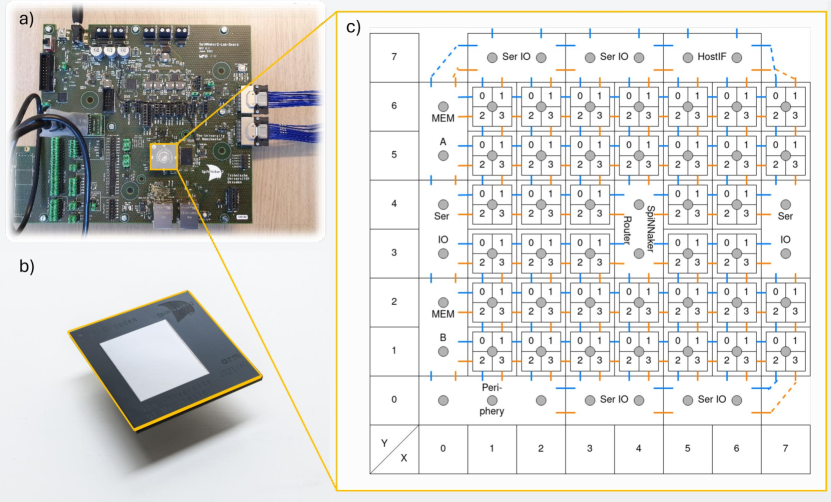
Figure S1: (a) Testing board used for the NeuroSA experiments, (b) highlighting its single SpiNNaker2 chip (c) and its internal topology.

The neuron model in NeuroSA is implemented through embedded software on SpiNNaker2 cores, while the high-level control and experiment configuration are performed through py-spinnaker2 [68], a Python library and high-level API designed for programming SpiNNaker2. Given an input MAX-CUT graph, we construct a NeuroSA network, where a mapper module within py-spinnaker2 determines the number of cores used as well as the distribution of neurons per core. This mapping depends on the network’s size, as measured by the number of neurons and synaptic connections. Following the architecture of the synchronous NeuroSA, as outlined in Methods section 3.4, we designed a global arbiter to perform the outer-loop level random selection across all active neurons at any time step. The arbiter uniformly samples one core ID from all used core IDs per time step. This selected core is the only core that is allowed to emit a spike at that time step. Following core selection, we update the membrane potentials for all neurons. Among neurons whose membrane potentials crossed the threshold on the selected core, the global arbiter uniformly samples only one neuron to spike. If none of the neurons on the selected core crossed the threshold, no spike is emitted at that time step. The uniform sampling of the cores as well as neurons that are selected for spike emission is done using the on-chip true random number generator [69]. Fig.  S2 depicts the firing dynamics of the NeuroSA implementation on SpiNNaker2.

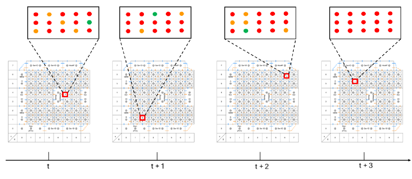
Figure S2: Overview of the random sampling of cores and neurons on SpiNNaker2. Each time step displays the internal topology of SpiNNaker2, with red squares indicating the selected core emitting a spike at that time step. Zooming in on the chosen reveals its neurons: those in red have not crossed the threshold, while those in yellow have. The green neuron signifies the spike emitter. At the final time step (t+3), no neurons have crossed the threshold, resulting in no spike emission.

S1.5 Effect of finite precision on NeuroSA

The evolution of the threshold $\mu$ is the key to the robustness of the NeuroSA architecture. While CPU (or software) implementation can use floating-point precision, in practice many neuromorphic hardware accelerators support only finite precision arithmetic. The long-term vision is to deploy NeuroSA on custom-ASIC or a hardware platform to achieve high energy-efficiency and low time-to-solution. One option is to implement the neuron and network model using standard neuromorphic architectures such as Loihi or SpiNNaker2, where as the FN annealers are realized in analog or using mixed-signal approaches using an analog-to-digital or digital-to-analog converters. Here we explore how the NeuroSA performance degrades when the precision of the computation is reduced. The state of the neurons are all binary variables taking values in $\{-1,+1\}$, where the weights (or connectivity) are also quantized. Therefore, the integrate-and-fire dynamics produces membrane potentials that are also discrete integers, however, their range and precision are limited by the network size and fan-out. Therefore, the only component in the architecture that is affected by quantization is the firing threshold for each neuron. We applied quantization to the thresholding function before determining the spiking activity of a particular neuron and plotted the obtained solution for each precision.

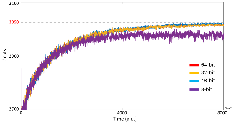
Figure S3: Effect of finite precision on the performance of NeuroSA.

As shown in Fig. S3, when quantized to 64- and 32-bit floating point, the noisy thresholds incurs identical neuron population dynamics, resulting in exactly the same evolution of the obtained results. When the precision is decreased to 16-bit the network dynamics differ from the high-precision cases but the overall performance in terms of solving the original optimization problem is similar, approaching the SOTA solution. However, when the precision is further decreased to 8-bit, the performance drops at the low-temperature region, as shown in Fig. S3 the purple curve. This result is as what we expected since the random fluctuation on the noisy threshold is vital to the performance of the NeuroSA architecture. When the temperature cools down, the amplitude of this fluctuation is also annealed. Under a low-precision scenario, the effect of the firing threshold fluctuation is concealed by the quantization effect. Therefore, the overall NeuroSA dynamics fail to follow the optimal simulated annealing dynamics which results in worse performance than the higher precision implementation.

S1.6 NeuroSA Low-temperature Start

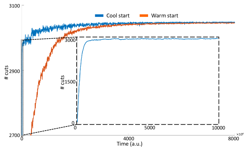
Figure S4: Using a low-temperature start to converge fast to a solution neighborhood, after which the annealing is used for exploring the solution space and asymptotic convergence to SOTA solution

From Eq. 2 and 13, if NeuroSA is configured with a low-temperature $T_{n}$ close to $0$, the update of neuron states is determined by the network gradient, which results in faster convergence. This is because during the initial stages of the dynamics, any stochastic factors slows down the convergence. As shown in Fig. S4, the cold-start condition pushes the network to convergence to $\sim 3000$ cuts for the $G15$ benchmark for which the SOTA is $3050$. However, the dynamics stalls after $\sim 10^{4}$ iterations because the network is trapped in the neighborhood of a local attractor state. However, by re-heating (or adding noise to the threshold) the solution can be further improved, as shown in Fig. S4. As indicated in Fig. 3e, the time to obtain a unit gain in solution takes up most of the entire duration, at the end of convergence. Therefore, the cold-start strategy accelerates only the initial phase of the optimization, and is intended for practical implementation when there is a simulation time constraint.

S1.7 Graph Maximum Fanouts/Latency

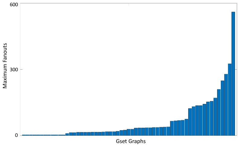
Figure S5: Maximum fanouts on each of the Gset benchmarks

The latency for propagating spiking events in a conventional sequential implementation of the NeuroSA architecture is determined by the latency between the spike generation to the time when all target neurons receive the spike and estimate the pseudo-gradient. Because of the simplicity of our neuron model design, the delay is mainly embedded in the sequential transmission of the spiking event, due to the shared bus in the system. Therefore, the maximum latency is determined by the largest fanout in the problem graph. As indicated in Fig. S5, the maximum fanout among all tested Gset graphs is around $600$, indicating a consecutive $600$ incidents of routing the spiking events across the system interconnect. On the other hand, in neuromorphic hardware, where the neurons are implemented in parallel and distributed across the network, the transmission delay is offset by the large fanout of the physical interconnects between neuron pairs. Therefore, the neuromorphic implementation is not limited by fanout of the graph.

S1.8 Table of Comparison for Gset Benchmarks

The tables 1 and 2 summarize the SOTA solution reported for different Gset benchmarks [55] and the difference from the worst-case solution obtained by NeuroSA.

Table 1: Gset1-30 Results

Gset Benchmarks	SOTA Solution	NeuroSA
G1	11624	0
G2	11620	-3
G3	11622	0
G4	11646	-5
G5	11631	0
G6	2178	0
G7	2006	0
G10	2000	-1
G11	564	0
G12	556	0
G13	582	0
G14	3064	-1
G15	3050	-1
G16	3052	0
G17	3047	-2
G18	992	-4
G19	906	-1
G20	941	0
G21	931	-3
G22	13359	-1
G23	13344	-3
G24	13337	-2
G25	13340	-7
G26	13328	-4
G27	3341	0
G28	3298	-2
G29	3405	-14
G30	3413	-1

Table 2: Gset 31-59, 67, 72 Results

Gset Benchmarks	SOTA Solution	NeuroSA
G31	3310	-2
G32	1410	-4
G33	1382	-2
G34	1384	-2
G35	7687	-12
G36	7680	-17
G37	7691	-8
G38	7688	-16
G39	2408	-3
G40	2400	-7
G41	2405	-12
G42	2481	-15
G43	6660	0
G44	6650	0
G45	6654	0
G46	6649	-3
G47	6657	-1
G48	6000	0
G49	6000	0
G50	5880	0
G51	3848	-1
G52	3851	-4
G53	3850	0
G54	3852	-4
G55	10299	-15
G56	4017	-11
G57	3494	-22
G58	19293	-39
G59	6086	-31
G67	6950	-68
G72	7006	-76

References

- \bibcommenthead
- Barahona [1982] Barahona, F.: On the computational complexity of ising spin glass models. Journal of Physics A: Mathematical and General 15(10), 3241 (1982) https://doi.org/10.1088/0305-4470/15/10/028
- Lucas [2014] Lucas, A.: Ising formulations of many np problems. Frontiers in Physics 2 (2014) https://doi.org/10.3389/fphy.2014.00005
- Mohseni et al. [2022] Mohseni, N., McMahon, P.L., Byrnes, T.: Ising machines as hardware solvers of combinatorial optimization problems. Nature Reviews Physics 4(6), 363–379 (2022) https://doi.org/10.1038/s42254-022-00440-8
- Hamerly et al. [2019] Hamerly, R., Inagaki, T., McMahon, P.L., Venturelli, D., Marandi, A., Onodera, T., Ng, E., Langrock, C., Inaba, K., Honjo, T., et al.: Experimental investigation of performance differences between coherent ising machines and a quantum annealer. Science advances 5(5), 0823 (2019)
- Tanahashi et al. [2019] Tanahashi, K., Takayanagi, S., Motohashi, T., Tanaka, S.: Application of ising machines and a software development for ising machines. Journal of the Physical Society of Japan 88(6), 061010 (2019)
- King et al. [2022] King, A.D., Suzuki, S., Raymond, J., Zucca, A., Lanting, T., Altomare, F., Berkley, A.J., Ejtemaee, S., Hoskinson, E., Huang, S., Ladizinsky, E., MacDonald, A.J.R., Marsden, G., Oh, T., Poulin-Lamarre, G., Reis, M., Rich, C., Sato, Y., Whittaker, J.D., Yao, J., Harris, R., Lidar, D.A., Nishimori, H., Amin, M.H.: Coherent quantum annealing in a programmable 2,000 qubit ising chain. Nature Physics 18(11), 1324–1328 (2022) https://doi.org/10.1038/s41567-022-01741-6
- Cen et al. [2022] Cen, Q., Ding, H., Hao, T., Guan, S., Qin, Z., Lyu, J., Li, W., Zhu, N., Xu, K., Dai, Y., Li, M.: Large-scale coherent ising machine based on optoelectronic parametric oscillator. Light: Science I& Applications 11 (2022) https://doi.org/10.1038/s41377-022-01013-1
- Mwamsojo et al. [2023] Mwamsojo, N., Lehmann, F., Merghem, K., Benkelfat, B.-E., Frignac, Y.: Optoelectronic coherent ising machine for combinatorial optimization problems. Opt. Lett. 48(8), 2150–2153 (2023) https://doi.org/10.1364/OL.485215
- Graber and Hofmann [2023] Graber, M., Hofmann, K.: An enhanced 1440 coupled cmos oscillator network to solve combinatorial optimization problems. In: 2023 IEEE 36th International System-on-Chip Conference (SOCC), pp. 1–6 (2023). https://doi.org/10.1109/SOCC58585.2023.10256945
- Maher et al. [2024] Maher, O., Jiménez, M., Delacour, C., Harnack, N., Núñez, J., Avedillo, M.J., Linares-Barranco, B., Todri-Sanial, A., Indiveri, G., Karg, S.: A cmos-compatible oscillation-based vo2 ising machine solver. Nature Communications 15(1), 3334 (2024) https://doi.org/10.1038/s41467-024-47642-5
- Cai et al. [2020] Cai, F., Kumar, S., Vaerenbergh, T.V., Sheng, X., Liu, R., Liu, R., Li, C., Liu, Z., Foltin, M., Yu, S., Xia, Q., Yang, J.J., Beausoleil, R.G., Lu, W., Strachan, J.P.: Power-efficient combinatorial optimization using intrinsic noise in memristor hopfield neural networks. Nature Electronics 3, 409–418 (2020) https://doi.org/10.1038/s41928-020-0436-6
- Jiang et al. [2023] Jiang, M., Shan, K., He, C., Li, C.: Efficient combinatorial optimization by quantum-inspired parallel annealing in analogue memristor crossbar. Nature Communications 14 (2023) https://doi.org/10.1038/s41467-023-41647-2
- Fahimi et al. [2021] Fahimi, Z., Mahmoodi, M., Nili, H., Polishchuk, V., Strukov, D.: Combinatorial optimization by weight annealing in memristive hopfield networks. Scientific Reports 11 (2021) https://doi.org/10.1038/s41598-020-78944-5
- Isakov et al. [2015] Isakov, S.V., Zintchenko, I.N., Rønnow, T.F., Troyer, M.: Optimised simulated annealing for ising spin glasses. Computer Physics Communications 192, 265–271 (2015) https://doi.org/10.1016/j.cpc.2015.02.015
- Kihara et al. [2017] Kihara, Y., Ito, M., Saito, T., Shiomura, M., Sakai, S., Shirakashi, J.: A new computing architecture using ising spin model implemented on fpga for solving combinatorial optimization problems. In: 2017 IEEE 17th International Conference on Nanotechnology (IEEE-NANO), pp. 256–258 (2017). IEEE
- Yamaoka et al. [2015] Yamaoka, M., Yoshimura, C., Hayashi, M., Okuyama, T., Aoki, H., Mizuno, H.: A 20k-spin ising chip to solve combinatorial optimization problems with cmos annealing. IEEE Journal of Solid-State Circuits 51(1), 303–309 (2015)
- Okuyama et al. [2016] Okuyama, T., Yoshimura, C., Hayashi, M., Yamaoka, M.: Computing architecture to perform approximated simulated annealing for ising models. In: 2016 IEEE International Conference on Rebooting Computing (ICRC), pp. 1–8 (2016). IEEE
- Kadowaki and Nishimori [1998] Kadowaki, T., Nishimori, H.: Quantum annealing in the transverse ising model. Physical Review E 58(5), 5355 (1998)
- Das and Chakrabarti [2008] Das, A., Chakrabarti, B.K.: Colloquium: Quantum annealing and analog quantum computation. Reviews of Modern Physics 80(3), 1061 (2008)
- Farhi et al. [2001] Farhi, E., Goldstone, J., Gutmann, S., Lapan, J., Lundgren, A., Preda, D.: A quantum adiabatic evolution algorithm applied to random instances of an np-complete problem. Science 292(5516), 472–475 (2001)
- Albash and Lidar [2018] Albash, T., Lidar, D.A.: Adiabatic quantum computation. Reviews of Modern Physics 90(1), 015002 (2018)
- Goto et al. [2019] Goto, H., Tatsumura, K., Dixon, A.R.: Combinatorial optimization by simulating adiabatic bifurcations in nonlinear hamiltonian systems. Science Advances 5(4), 2372 (2019) https://doi.org/10.1126/sciadv.aav2372 https://www.science.org/doi/pdf/10.1126/sciadv.aav2372
- Kang et al. [2020] Kang, M., Lee, Y., Park, M.: Energy efficiency of machine learning in embedded systems using neuromorphic hardware. Electronics 9(7), 1069 (2020)
- Ivanov et al. [2022] Ivanov, D., Chezhegov, A., Larionov, D.: Neuromorphic artificial intelligence systems. Frontiers in Neuroscience 16, 959626 (2022)
- Furber et al. [2014] Furber, S.B., Galluppi, F., Temple, S., Plana, L.A.: The spinnaker project. Proceedings of the IEEE 102(5), 652–665 (2014)
- Park et al. [2017] Park, J., Yu, T., Joshi, S., Maier, C., Cauwenberghs, G.: Hierarchical address event routing for reconfigurable large-scale neuromorphic systems. IEEE Transactions on Neural Networks and Learning Systems 28(10), 2408–2422 (2017) https://doi.org/10.1109/tnnls.2016.2572164
- Davies et al. [2018] Davies, M., Srinivasa, N., Lin, T.-H., Chinya, G., Cao, Y., Choday, S.H., Dimou, G., Joshi, P., Imam, N., Jain, S., et al.: Loihi: A neuromorphic manycore processor with on-chip learning. Ieee Micro 38(1), 82–99 (2018)
- Mayr et al. [2019] Mayr, C., Hoeppner, S., Furber, S.: Spinnaker 2: A 10 million core processor system for brain simulation and machine learning. arXiv preprint arXiv:1911.02385 (2019)
- Van Albada et al. [2018] Van Albada, S.J., Rowley, A.G., Senk, J., Hopkins, M., Schmidt, M., Stokes, A.B., Lester, D.R., Diesmann, M., Furber, S.B.: Performance comparison of the digital neuromorphic hardware spinnaker and the neural network simulation software nest for a full-scale cortical microcircuit model. Frontiers in neuroscience 12, 309524 (2018)
- Rhodes et al. [2020] Rhodes, O., Peres, L., Rowley, A.G., Gait, A., Plana, L.A., Brenninkmeijer, C., Furber, S.B.: Real-time cortical simulation on neuromorphic hardware. Philosophical Transactions of the Royal Society A 378(2164), 20190160 (2020)
- Liu et al. [2018] Liu, C., Bellec, G., Vogginger, B., Kappel, D., Partzsch, J., Neumärker, F., Höppner, S., Maass, W., Furber, S.B., Legenstein, R., et al.: Memory-efficient deep learning on a spinnaker 2 prototype. Frontiers in neuroscience 12, 416510 (2018)
- Lin et al. [2018] Lin, C.-K., Wild, A., Chinya, G.N., Cao, Y., Davies, M., Lavery, D.M., Wang, H.: Programming spiking neural networks on intel’s loihi. Computer 51(3), 52–61 (2018)
- Gonzalez et al. [2024] Gonzalez, H.A., Huang, J., Kelber, F., Nazeer, K.K., Langer, T., Liu, C., Lohrmann, M., Rostami, A., Schöne, M., Vogginger, B., et al.: Spinnaker2: A large-scale neuromorphic system for event-based and asynchronous machine learning. arXiv preprint arXiv:2401.04491 (2024)
- Shankar [2023] Shankar, S.: Energy estimates across layers of computing: From devices to large-scale applications in machine learning for natural language processing, scientific computing, and cryptocurrency mining. In: 2023 IEEE High Performance Extreme Computing Conference (HPEC), pp. 1–6 (2023). IEEE
- Hopfield [1982] Hopfield, J.J.: Neural networks and physical systems with emergent collective computational abilities. Proceedings of the national academy of sciences 79(8), 2554–2558 (1982)
- Friston [2010] Friston, K.: The free-energy principle: a unified brain theory? Nature reviews neuroscience 11(2), 127–138 (2010)
- Chialvo [2010] Chialvo, D.R.: Emergent complex neural dynamics. Nature physics 6(10), 744–750 (2010)
- Sompolinsky et al. [1988] Sompolinsky, H., Crisanti, A., Sommers, H.-J.: Chaos in random neural networks. Physical review letters 61(3), 259 (1988)
- McDonnell and Ward [2011] McDonnell, M.D., Ward, L.M.: The benefits of noise in neural systems: bridging theory and experiment. Nature Reviews Neuroscience 12(7), 415–425 (2011)
- Schneidman et al. [1998] Schneidman, E., Freedman, B., Segev, I.: Ion channel stochasticity may be critical in determining the reliability and precision of spike timing. Neural computation 10(7), 1679–1703 (1998)
- Branco et al. [2008] Branco, T., Staras, K., Darcy, K.J., Goda, Y.: Local dendritic activity sets release probability at hippocampal synapses. Neuron 59(3), 475–485 (2008)
- Jaeger and Haas [2004] Jaeger, H., Haas, H.: Harnessing nonlinearity: Predicting chaotic systems and saving energy in wireless communication. science 304(5667), 78–80 (2004)
- Hoppensteadt and Izhikevich [1999] Hoppensteadt, F.C., Izhikevich, E.M.: Oscillatory neurocomputers with dynamic connectivity. Physical Review Letters 82(14), 2983 (1999)
- Fischer and Igel [2012] Fischer, A., Igel, C.: An introduction to restricted boltzmann machines. In: Progress in Pattern Recognition, Image Analysis, Computer Vision, and Applications: 17th Iberoamerican Congress, CIARP 2012, Buenos Aires, Argentina, September 3-6, 2012. Proceedings 17, pp. 14–36 (2012). Springer
- Amin et al. [2018] Amin, M.H., Andriyash, E., Rolfe, J., Kulchytskyy, B., Melko, R.: Quantum boltzmann machine. Physical Review X 8(2), 021050 (2018)
- Mehta et al. [2022] Mehta, D., Rahman, M., Aono, K., Chakrabartty, S.: An adaptive synaptic array using fowler–nordheim dynamic analog memory. Nature Communications 13(1) (2022) https://doi.org/10.1038/s41467-022-29320-6
- Smith et al. [2022] Smith, J.D., Hill, A.J., Reeder, L.E., Franke, B.C., Lehoucq, R.B., Parekh, O., Severa, W., Aimone, J.B.: Neuromorphic scaling advantages for energy-efficient random walk computations. Nature Electronics 5(2), 102–112 (2022) https://doi.org/10.1038/s41928-021-00705-7
- Goemans and Williamson [1995] Goemans, M.X., Williamson, D.P.: Improved approximation algorithms for maximum cut and satisfiability problems using semidefinite programming. Journal of the ACM (JACM) 42(6), 1115–1145 (1995)
- Kirkpatrick et al. [1983] Kirkpatrick, S., Gelatt, C.D., Vecchi, M.P.: Optimization by simulated annealing. Science 220(4598), 671–680 (1983) https://doi.org/10.1126/science.220.4598.671
- Geman and Geman [1984] Geman, S., Geman, D.: Stochastic relaxation, gibbs distributions, and the bayesian restoration of images. IEEE Transactions on pattern analysis and machine intelligence (6), 721–741 (1984)
- Hajek [1988] Hajek, B.: Cooling schedules for optimal annealing. Mathematics of Operations Research 13(2), 311–329 (1988). Accessed 2024-04-11
- Lucas [2014] Lucas, A.: Ising formulations of many np problems. Frontiers in physics 2, 74887 (2014)
- Fowler and Nordheim [1928] Fowler, R.H., Nordheim, L.: Electron Emission in Intense Electric Fields. Proceedings of the Royal Society of London Series A 119(781), 173–181 (1928) https://doi.org/10.1098/rspa.1928.0091
- Zhou and Chakrabartty [2017] Zhou, L., Chakrabartty, S.: Self-powered timekeeping and synchronization using fowler–nordheim tunneling-based floating-gate integrators. IEEE Transactions on Electron Devices 64(3), 1254–1260 (2017) https://doi.org/%****␣sn-article.bbl␣Line␣900␣****10.1109/TED.2016.2645379
- [55] Matsuda, Y.: Benchmarking the MAX-CUT problem on the Simulated Bifurcation Machine — medium.com. https://medium.com/toshiba-sbm/benchmarking-the-max-cut-problem-on-the-simulated-bifurcation-machine-e26e1127c0b0. [Accessed 20-04-2024]
- Tanahashi et al. [2019] Tanahashi, K., Takayanagi, S., Motohashi, T., Tanaka, S.: Application of ising machines and a software development for ising machines. Journal of the Physical Society of Japan 88(6), 061010 (2019)
- Stopfer et al. [2003] Stopfer, M., Jayaraman, V., Laurent, G.: Intensity versus identity coding in an olfactory system. Neuron 39(6), 991–1004 (2003)
- Layden et al. [2023] Layden, D., Mazzola, G., Mishmash, R.V., Motta, M., Wocjan, P., Kim, J.-S., Sheldon, S.: Quantum-enhanced markov chain monte carlo. Nature 619(7969), 282–287 (2023) https://doi.org/10.1038/s41586-023-06095-4
- Ye [2003] Ye, Y.: The Gset Dataset. https://web.stanford.edu/~yyye/yyye/Gset/ (2003)
- Dehmer and Mowshowitz [2011] Dehmer, M., Mowshowitz, A.: A history of graph entropy measures. Information Sciences 181(1), 57–78 (2011)
- Holland and Leinhardt [1971] Holland, P.W., Leinhardt, S.: Transitivity in structural models of small groups. Comparative group studies 2(2), 107–124 (1971)
- Rueckauer et al. [2017] Rueckauer, B., Lungu, I.-A., Hu, Y., Pfeiffer, M., Liu, S.-C.: Conversion of continuous-valued deep networks to efficient event-driven networks for image classification. Frontiers in Neuroscience 11 (2017) https://doi.org/10.3389/fnins.2017.00682
- Friedrich and Laurent [2001] Friedrich, R.W., Laurent, G.: Dynamic optimization of odor representations by slow temporal patterning of mitral cell activity. Science 291(5505), 889–894 (2001)
- Gangopadhyay and Chakrabartty [2021] Gangopadhyay, A., Chakrabartty, S.: A sparsity-driven backpropagation-less learning framework using populations of spiking growth transform neurons. Frontiers in neuroscience 15, 715451 (2021)
- Ozaeta et al. [2022] Ozaeta, A., Dam, W., McMahon, P.L.: Expectation values from the single-layer quantum approximate optimization algorithm on ising problems. Quantum Science and Technology 7(4), 045036 (2022) https://doi.org/10.1088/2058-9565/ac9013
- Pierog et al. [2015] Pierog, T., Karpenko, I., Katzy, J.M., Yatsenko, E., Werner, K.: Epos lhc: Test of collective hadronization with data measured at the cern large hadron collider. Phys. Rev. C 92, 034906 (2015) https://doi.org/10.1103/PhysRevC.92.034906
- Mehta D. [2020] Mehta D., C.S. Aono A.: A self-powered analog sensor-data-logging device based on fowler-nordheim dynamical systems. Nature Communications 11(5446) (2020) https://doi.org/10.1038/s41467-020-19292-w
- Vogginger et al. [2023] Vogginger, B., Kelber, F., Jobst, M., Yan, Y., Gerhards, P., Weih, M., Akl, M.: Py-spinnaker2. https://doi.org/10.5281/zenodo.10202110 . https://doi.org/10.5281/zenodo.10202110
- Neumarker et al. [2016] Neumarker, F., Höppner, S., Dixius, A., Mayr, C.: True random number generation from bang-bang adpll jitter. In: 2016 IEEE Nordic Circuits and Systems Conference (NORCAS), pp. 1–5 (2016). https://doi.org/10.1109/NORCHIP.2016.7792875