Numerically robust square root implementations of statistical linear regression filters and smoothers

Abstract

In this article, square-root formulations of the statistical linear regression filter and smoother are developed. Crucially, the method uses QR decompositions rather than Cholesky downdates. This makes the method inherently more numerically robust than the downdate based methods, which may fail in the face of rounding errors. This increased robustness is demonstrated in an ill-conditioned problem, where it is compared against a reference implementation in both double and single precision arithmetic. The new implementation is found to be more robust, when implemented in lower precision arithmetic as compared to the alternative.

I Introduction

Consider the probabilistic state-space model given by

$$x_{0} \sim\mathcal{N}(\mu_{0},\Sigma_{0}),$$ (1a)

$$x_{m}\mid x_{m-1} \sim\mathcal{N}(f(x_{m-1}),Q(x_{m-1})),$$ (1b)

$$y_{m}\mid x_{m} \sim\mathcal{N}(c(x_{m}),R(x_{m})),$$ (1c)

where $f$ is the transition function, $Q$ the transition covariance, $c$ the observation function, $R$ the observation covariance. The vector $x_{m}$ is the latent and $y_{m}$ is an imperfect observation of the former. Let $\pi_{m\mid 1\mathrel{\mathop{\ordinarycolon}}k}$ denote the following conditional density

$$\pi_{m\mid 1\mathrel{\mathop{\ordinarycolon}}k}(x)=\pi(x_{m}\mid y_{1\mathrel{\mathop{\ordinarycolon}}k})$$

so that the filtering density at time $m$ is given by $\pi_{m\mid 1\mathrel{\mathop{\ordinarycolon}}m}$ and the smoothing density based on measurements $y_{1},\ldots,y_{n}$ is given by $\pi_{m\mid 1\mathrel{\mathop{\ordinarycolon}}n}$ for $m\leq n$.

The filtering density, $\pi_{m\mid 1\mathrel{\mathop{\ordinarycolon}}m}$, satisfies the following prediction/correction recursion [1, 2]

$$\pi_{m+1\mid 1\mathrel{\mathop{\ordinarycolon}}m}(x)=\int\mathcal{N}(x;f(x^{\prime}),Q(x^{\prime}))\pi_{m\mid 1\mathrel{\mathop{\ordinarycolon}}m}(x^{\prime})\operatorname{d\!}x^{\prime},$$

$$\pi_{m+1\mid 1\mathrel{\mathop{\ordinarycolon}}m+1}(x)=\frac{\mathcal{N}(y;c(x),R(x))\pi_{m+1\mid 1\mathrel{\mathop{\ordinarycolon}}m}(x)}{\int\mathcal{N}(y;c(x^{\prime}),R(x^{\prime}))\pi_{m+1\mid 1\mathrel{\mathop{\ordinarycolon}}m}(x^{\prime})\operatorname{d\!}x^{\prime}}.$$

Now define backward transition density $b_{m\mid m+1}$:

$$b_{m\mid m+1}(x\mid x^{\prime})=\frac{\pi_{m\mid 1\mathrel{\mathop{\ordinarycolon}}m}(x)\mathcal{N}(x^{\prime};f(x),Q(x))}{\pi_{m+1\mid 1\mathrel{\mathop{\ordinarycolon}}m}(x^{\prime})},$$ (3)

then the smoothing density follows the following, backward, recursion [3, 4]

$$\pi_{m\mid 1\mathrel{\mathop{\ordinarycolon}}n}(x)=\int b_{m\mid m+1}(x\mid x^{\prime})\pi_{m+1\mid 1\mathrel{\mathop{\ordinarycolon}}n}(x^{\prime})\operatorname{d\!}x^{\prime}.$$

It may be noted that $b_{m\mid m+1}(x\mid x^{\prime})$ is simply Bayes’ rule when the prior is $\pi_{m\mid 1\mathrel{\mathop{\ordinarycolon}}m}(x)$ and the likelihood is $\mathcal{N}(x^{\prime};f(x),Q(x))$.

The problem of Bayesian filtering and smoothing for linear Gaussian models was largely solved by the development of the Kalman filter and Rauch–Tung–Striebel smoother [6, 7]. However, the non-linear case is intractable in general, hence the flourishing field of approximate inference [2].

Perhaps the earliest approach was based on linearization by Taylor series, leading to the extended Kalman filter (EKF) [8]. This thinking lead to the optimization based direction in approximate state estimation [9, 10, 11, 12, 13].

Later on, alternative approaches were devised based on cubature based moment approximation and linear minimum mean square error estimation [14, 15, 16, 17, 18]. The cubature approach has been shown to be equivalent to an alternative linearization strategy termed statistical linear regression [19, 20].

Taking inspiration from the optimization based viewpoint, iterative variants of the statistical linear regression method have been developed [21, 22, 23, 24, 25, 26]. Iterative statistical linear regression has also found applications in importance density design [27] and Gaussian process classification [28].

When the covariance matrices are ill-conditioned, the Ricatti recursion for the covariance in linear state estimators is prone to numerical instability. This lead to the development of recursions for the square-root of the covariance matrix instead [29, 8, 30]. The reader may consult [8] for a catalog of such approaches. Because Taylor linearization does not modify the covariance matrix, this trivially extends to the EKF. Various square root methods have also been employed for the cubature based methods [31, 32, 33, 34, 35, 36]. However, analogous methods for statistical linear regression based estimators have not been examined to the same extent. As far as we are aware, the only contribution in this direction is given by [37], which proposes a method based on sequential updating and downdating. However, the downdating problem can be ill-conditioned [38, 39, 40], and may fail completely due to round off errors [36].

Other notable solutions to the state estimation problem are the projection based approach [41], variational inference [42, 43], and sequential Monte Carlo [44, 45, 46, 47, 48, 49]. However, they fall outside of the scope of the present discussion.

I-A Contribution

This article develops an approach for implementing statistical linear regression based state estimators in square root form. In contrast to [37], the proposed method does not rely on Cholesky downdates, but rather QR decompositions. Consequently, the proposed algorithm is expected to remain numerically reliable when the state estimation problem is ill-conditioned or when the state estimation algorithm is implemented in low precision arithmetic, whereas Cholesky downdates may fail [36].

I-B Notation

For a matrix $A$, its adjoint is denoted by $A^{*}$. For a positive definite matrix $\Pi$, its lower triangular Cholesky factor is denoted by $\Pi^{1/2}$ so that $\Pi=\Pi^{1/2}\Pi^{*/2}$, where $\Pi^{*/2}$ is the upper triangular Cholesky factor. Furthermore, for matrices $A_{1}$ and $A_{2}$ the relation $A_{1}\cong A_{2}$ holds if and only if $A_{1}^{*}A_{1}=A_{2}^{*}A_{2}$. In particular, $A_{1}\cong(A_{1}^{*}A_{1})^{*/2}$, and a Cholesky factor of $A_{1}^{*}A_{1}$ may thus be obtained by taking the upper triangular factor in the QR decomposition of $A_{1}$.

II Gaussian state estimation in square-root form

In this section, the square root implementations of Gaussian state estimators is summarized. That is, filtering and smoothing the following model.

$$x_{m}\mid x_{m-1} \sim\mathcal{N}(\Phi_{m}x_{m-1},Q_{m}),$$ (4a)

$$y_{m}\mid x_{m} \sim\mathcal{N}(C_{m}x_{m},R_{m}).$$ (4b)

The following lemma is fundamental for the implementation of square-root based filters and smoothers in linear Gaussian models [30, Chapter 6].

Lemma 1.

The model following model

$$u \sim\mathcal{N}(\bar{u},\Pi),$$

$$v\mid u \sim\mathcal{N}(\Psi u,\Omega),$$

is equivalent to

$$v \sim\mathcal{N}(C\bar{u},P),$$

$$u\mid v \sim\mathcal{N}(\bar{u}+\Gamma(v-\Psi\bar{u}),\Sigma),$$

where the parameters $P,\Gamma$, and $\Sigma$ are given by

$$\begin{pmatrix}\Omega^{*/2}&0\\ \Pi^{*/2}\Psi^{*}&\Pi^{*/2}\end{pmatrix} \cong\begin{pmatrix}P^{*/2}&\bar{\Gamma}^{*}\\ 0&\Sigma^{*/2}\end{pmatrix},$$ (5)

$$\Gamma =\bar{\Gamma}P^{-1/2}.$$ (6)

The interpretation of lemma 1 is as follows. When $u=x_{n}$, $\bar{u}$ and $\Pi$ are the respective moments of the predictive distribution, and $v=y_{n}$, then lemma 1 provides a way to compute the Cholesky factors of the filtering and marginal measurement covariances, and filter gain by just one QR decomposition and one linear solve with respect to $P^{1/2}$ (the Cholesky factor of the marginal measurement covariance).

Similarly, when $u=x_{n-1}$, $\bar{u}$ and $\Pi$ are the respective moments of the filtering distribution distribution, and $v=x_{n}$, then lemma 1 provides a way to compute the Cholesky factors of the predictive and backward process covariances (the covariance of (3)), and smoother gain by just one QR decomposition and one linear solve with respect to $P^{1/2}$ (the Cholesky factor of the predictive covariance).

It is important to note that lemma 1 only requires one linear solve with the Cholesky factor of $P$, rather than two which is required in the cubature approaches of [18, 50]. Consequently, if statistical linear regression can be used to directly obtain a Cholesky factor of $P$, then it can be expected to be more numerically robust when $P$ is ill-conditioned.

III Statistical linear regression in square root form

In this section, a method for implementing the statistical linear regression algorithm in square root form is developed. In contrast to the method of [37], it does not make use of Cholesky downdates but employs QR decompositions instead (equivalent to Cholesky updates).

III-A Statistical linear regression

The statistical linear regression problem is concerned with finding a linear Gaussian approximation to the conditional density in the following model [19]

$$u \sim\mathcal{N}(\bar{u},\Pi),$$ (7)

$$v\mid u \sim\mathcal{N}(a(u),\Omega),$$ (8)

by the following minimization problem

$$e_{\Psi_{0},b_{0}}(u,v) =v-\Psi_{0}u-b_{0},$$

$$\bar{\Psi},\bar{b} =\arg\,\min_{\Psi_{0},b_{0}}\,\mathbb{E}\Big{[}\mathinner{\!\left\lvert e_{\Psi_{0},b_{0}}(u,v)\right\rvert}^{2}\Big{]}.$$

Let $\bar{e}(u,v)=e_{\bar{\Psi},\bar{b}}(u,v)$, then the residual covariance matrix is given by

$$\bar{\Omega}=\mathbb{E}[\bar{e}(u,v)\bar{e}^{*}(u,v)].$$ (10)

This results in the following Gaussian approximation [21, 22]

$$\mathcal{N}(a(u),\Omega)\approx\mathcal{N}(\bar{\Psi}u+\bar{b},\bar{\Omega}).$$

The solution to the statistical linear regression problem is given by [19, 21, 22]

$$\bar{a} =\mathbb{E}[a(u)],$$ (11a)

$$\bar{\Psi} =\mathbb{E}[a(u)(u-\bar{u})^{*}]\Pi^{-1},$$ (11b)

$$\bar{b} =\bar{a}-\bar{\Psi}\bar{u},$$ (11c)

$$\bar{\Omega} =\Omega+\mathbb{E}[(a(u)-\bar{a})(a(u)-\bar{a})^{*}]-\bar{\Psi}\Pi\bar{\Psi}^{*}.$$ (11d)

III-B Cubature implementation of statistical linear regression

The expectations in (11) are generally intractable. They can be transformed to integration with respect to a standard Gaussian by change of variables

$$z=\Pi^{-1/2}(u-\bar{u}).$$ (12)

Thus for an arbitrary function $\varphi$, its expectation is given by

$$\mathbb{E}[\varphi(u)]=\mathbb{E}[\varphi(\bar{u}+\Pi^{1/2}z)].$$

One way of approximating these expectations is thus to take a cubature rule with respect to the standard Gaussian, using $p$ nodes, with weights and nodes given by

$$w =\begin{pmatrix}w_{1}&\ldots&w_{p}\end{pmatrix},$$

$$Z =\begin{pmatrix}z_{1},\ldots,z_{p}\end{pmatrix}.$$

This is then transformed into a cubature rule, $(w,U)$, with respect $\mathcal{N}(u;\bar{u},\Pi)$ via (12) according to

$$\Delta u_{i} =\Pi^{1/2}z_{i},$$ (14a)

$$u_{i} =\bar{u}+\Delta u_{i},$$ (14b)

where the $i$th column of $U$ us $u_{i}$. The expectation of an arbitrary function $\varphi$, is then approximated by

$$\mathbb{E}[\varphi(u)]\approx\sum_{i=1}^{p}w_{i}\varphi(u_{i}).$$

Now, define the following quantities

$$W =\operatorname{diag}w$$ (15a)

$$\Delta U =\begin{pmatrix}\Delta u_{1},\ldots,\Delta u_{p}\end{pmatrix},$$ (15b)

$$A =\begin{pmatrix}a(u_{1}),\ldots,a(u_{p})\end{pmatrix},$$ (15c)

$$\Delta A =\begin{pmatrix}a(u_{1})-\bar{a},\ldots,a(u_{p})-\bar{a}\end{pmatrix}.$$ (15d)

An approximate solution to the statistical linear regression problem is then given by

$$\bar{a} =Aw,$$ (16a)

$$\bar{\Psi} =\Delta AW\Delta U^{*}\Pi^{-1},$$ (16b)

$$\bar{b} =\bar{a}-\bar{\Psi}\bar{u},$$ (16c)

and the residual covariance matrix is approximated by

$$\bar{\Omega}=\Omega+\Delta AW\Delta A^{*}-\bar{\Psi}\Pi\bar{\Psi}^{*}.$$ (17)

III-C Square root implementation of statistical linear regression

In this section, a downdate free method for implementing the statistical linear regression algorithm is developed. The following assumption on the chosen cubature rule is required.

Assumption 1.

The cubature rule with nodes $\{u_{i}\}_{i=1}^{p}$ and weights $\{w_{i}\}_{i=1}^{p}$ for $\mathcal{N}(\mu,\Pi)$ satisfy the following:

• It is polynomially exact of at least degree 2.

• The weights are positive.

Assumption 1 is satisfied by for example Gauss–Hermite quadrautre [15] or spherical radial cubature [18]. It does not in general hold for the unscented transform [16], since for some parameters it has a negative weight [2].

Proposition 1.

Let $\{x_{i}\}_{i=1}^{p}$ and $\{w_{i}\}_{i=1}^{p}$ be a cubature rule for $\mathcal{N}(\mu,\Pi)$ that satisfy assumption 1. Define the matrix:

$$E=\Delta A-\bar{\Psi}\Delta U,$$

then $\bar{\Omega}$ is given by

$$\bar{\Omega}=\Omega+EWE^{*}.$$ (18)

Proof.

By direct calculation from the definition of $E$

$$\begin{split}EWE^{*}&=(\Delta A-\bar{\Psi}\Delta U)W(\Delta A-\bar{\Psi}\Delta U)^{*}\\ &=\Delta AW\Delta A^{*}-\Delta AW\Delta U^{*}\bar{\Psi}^{*}\\ &\quad-\bar{\Psi}\Delta UW\Delta A^{*}+\bar{\Psi}\Delta UW\Delta U^{*}\bar{\Psi}^{*}\end{split}$$

and by (16) $\Delta AW\Delta U^{*}=\bar{\Psi}\Pi$, hence

$$EWE^{*}=\Delta AW\Delta A^{*}-2\bar{\Psi}\Pi\bar{\Psi}^{*}+\bar{\Psi}\Delta UW\Delta U^{*}\bar{\Psi}^{*}.$$

Furthermore, by assumption 1 (polynomial exactness of at least degree 2) $\Delta UW\Delta U^{*}=\Pi$, therefore

$$EWE^{*}=\Delta AW\Delta A^{*}-\bar{\Psi}\Pi\bar{\Psi}^{*}.$$

In view of (17), adding $\Omega$ to both sides of the previous equation gives the desired conclusion. ∎

Proposition 1 suggests that $\bar{\Omega}$ may be computed with only updates. This is readily verified since assumption 1 ensures that $W$ is positive definite, and consequently $W^{1/2}$ is well-defined.

Corollary 1.

With assumption 1 still in effect, the matrix $\bar{\Omega}$ admits the following factorization

$$\bar{\Omega}^{*/2}\cong\begin{pmatrix}\Omega^{1/2}&EW^{1/2}\end{pmatrix}^{*}.$$ (19)

In view of corollary 1, a Cholesky factor of $\bar{\Omega}$ may be obtained by taking the upper triangular part in the QR decomposition of the right-hand side of (19).

III-D Extension to state-dependent noise

An extension to state-dependent noise, $\Omega=\Omega(u)$, can be obtained provided there is a numerically safe way to evaluate $\Omega^{1/2}(u)$ [37]. In this case, the cubature approximation of the residual covariance matrix is given by (c.f. [23])

$$\bar{\Omega}=\sum_{i=1}^{p}w_{i}\Omega(u_{i})+\sum_{i=1}^{p}\Delta AW\Delta A^{*}-\bar{\Psi}\Pi\bar{\Psi}^{*},$$

which by proposition 1 simplifies to

$$\bar{\Omega}=\sum_{i=1}^{p}w_{i}\Omega(u_{i})+EWE^{*}.$$ (20)

The Cholesky factor of $\bar{\Omega}^{*/2}$ may then be obtained by taking the upper triangular factor in the QR decomposition of

$$\begin{pmatrix}EW^{1/2}&\sqrt{w_{1}}\Omega^{1/2}(u_{i})&\ldots&\sqrt{w_{p}}\Omega^{1/2}(u_{p})\end{pmatrix}^{*}.$$ (21)

IV Experimental results

Consider the continuous-time coordinated turn model [51]

$$\operatorname{d\!}\begin{pmatrix}p(t)\\ \dot{p}(t)\\ \omega(t)\end{pmatrix}=\begin{pmatrix}\dot{p}(t)\operatorname{d\!}t\\ \omega(t)Jp(t)\operatorname{d\!}t+B_{0}\operatorname{d\!}w_{p}(t)\\ \sigma_{\omega}\operatorname{d\!}w_{\omega}(t)\end{pmatrix},$$ (22)

where $p$ is the position, $\dot{p}$ is the velocity, and $\omega$ is the turn rate. The matrices $J$ and $B_{0}$ are given by

$$J=\begin{pmatrix}0&-1\\ 1&0\end{pmatrix},\quad B_{0}=\operatorname{diag}(\sigma_{x},\sigma_{y}).$$

and $w_{p},w_{\omega}$ are standard Wiener processes of appropriate dimension. An approximation may be obtained by holding $\omega$ dependence of the drift fixed during sampling intervals so that the model is linear on $[t_{m-1},t_{m}]$ conditionally on $\omega(t_{m-1})$. The approximate model may then be written as

$$\operatorname{d\!}x(t)=A(\omega(t_{m-1}))x(t)\operatorname{d\!}t+B\operatorname{d\!}w(t),\quad t\in[t_{m-1},t_{m}),$$

where the definition of $A$ and $B$ are clear from (22). This results in the transition following densities

$$\mathcal{N}\Big{(}e^{A(\omega(t_{m-1}))(t_{m}-t_{m-1})}x(t_{m-1}),Q(\omega(t_{m-1}),t_{m}-t_{m-1})\Big{)}.$$

Both the matrix exponential and a Cholesky factor of $Q(\omega(t_{m-1}),t_{m}-t_{m-1})$ may be computed to high precision by the algorithm of [52]. This leads to a variant of the model used by [18], that is more faithful to the continuous time dynamics. The initial state distribution is Gaussian with parameters

$$\mu_{0} =\begin{pmatrix}1000.0&1000.0&300.0&0.0&-0.0523\end{pmatrix},$$

$$\Sigma_{0} =\operatorname{diag}\begin{pmatrix}10.0&10.0&3.162&3.162&0.316\end{pmatrix},$$

the sampling interval is fixed, $\delta t=t_{m}-t_{m-1}$, and the dynamics parameters are set to

$$\delta t=1,\quad\sigma_{x}=\sigma_{y}=0.03,\quad\sigma_{\omega}=0.013.$$

The state is measured according to

$$\begin{pmatrix}r(t_{m})\\ \theta(t_{m})\end{pmatrix}=\begin{pmatrix}\mathinner{\!\left\lVert p(t_{m})\right\rVert}+w_{r}(t_{m})\\ \tan^{-1}(p_{2}(t_{m}),p_{1}(t_{m}))+w_{\theta}(t_{m})\end{pmatrix},$$

where $w_{r}(t_{m})$ and $w_{\theta}(t_{m})$ are zero mean Gaussian distributed with standard deviations $\sigma_{r}$ and $\sigma_{\theta}$, respectively, given by

$$\sigma_{r}=10,\quad\sigma_{\theta}=0.0031.$$

The proposed implementation (prop) is compared against a reference implementation [37] (ref) by solving the smoothing problem using and iterative statistical linear regression based smoother with 10 iterations [22, 23]. The comparison is made in both single and double precision floating point arithmetic. The norm of the errors in $p(t_{m})$, $\dot{p}(t_{m})$, and $\omega(t_{m})$ are recorded over 100 Monte Carlo generated trajectories of length 101.

The results are shown in figure 1 for the proposed method in both single and double precision arithmetic. The reference implementation is only shown for double precision as it fails in single precision, due to Cholesky downdates. As can be seen from the figure, the errors are indistinguishable. This suggests the proposed implementation ought to be preferred as it more robust to ill-conditioning / low precision arithmetic.

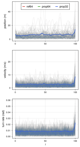
Figure 1: The errors in position (top), velocity (middle), and turn rate (bottom), for the reference implementation [37] (ref) and the proposed implementation (prop). The average errors across Monte Carlo trials is shown in solid, whereas the error for each trial is shown in transparent color. The floating point precision used by the algorithm is indicated in the legend by 32 and 64 for single double precision, respectively. Note that the results of the algorithms are completely indistinguishable. Except for ref32 which can not run at all because of failing Cholesky downdates, hence its absence in the figure.

V Conclusion

In this article, we have shown that statistical linear regression in square root form can be implemented in a numerically robust way and demonstrated its positive impact on tracking performance in an ill-conditioned problem, where the present best implementation by [37] fails in single precision arithmetic.

References

- [1] Y. Ho and R. Lee, “A Bayesian approach to problems in stochastic estimation and control,” IEEE Transactions on Automatic Control, vol. 9, no. 4, pp. 333–339, 1964.
- [2] S. Särkkä and L. Svensson, Bayesian Filtering and Smoothing. Cambridge university press, 2023, vol. 17.
- [3] G. Kitagawa, “Non-Gaussian state—space modeling of nonstationary time series,” Journal of the American Statistical Association, vol. 82, no. 400, pp. 1032–1041, 1987.
- [4] O. Cappé, E. Moulines, and T. Rydén, Inference in Hidden Markov Models. Springer, 2005.
- [5] F. Tronarp, N. Bosch, and P. Hennig, “Fenrir: Physics-enhanced regression for initial value problems,” in International Conference on Machine Learning. PMLR, 2022, pp. 21 776–21 794.
- [6] R. E. Kalman, “New results in linear filtering and prediction theory,” Transactions of the ASME, Journal of Basic Engineering, vol. 82, pp. 35–45, 1961.
- [7] H. E. Rauch, F. Tung, and C. T. Striebel, “Maximum likelihood estimates of linear dynamic systems,” AIAA journal, vol. 3, no. 8, pp. 1445–1450, 1965.
- [8] T. Kailath, A. H. Sayed, and B. Hassibi, Linear estimation. Prentice Hall, 2000.
- [9] B. M. Bell and F. W. Cathey, “The iterated Kalman filter update as a Gauss-Newton method,” IEEE Transactions on Automatic Control, vol. 38, no. 2, pp. 294–297, 1993.
- [10] B. M. Bell, “The iterated Kalman smoother as a Gauss–Newton method,” SIAM Journal on Optimization, vol. 4, no. 3, pp. 626–636, 1994.
- [11] M. A. Skoglund, G. Hendeby, and D. Axehill, “Extended Kalman filter modifications based on an optimization view point,” in 2015 18th International Conference on Information Fusion (Fusion). IEEE, 2015, pp. 1856–1861.
- [12] A. Aravkin, J. V. Burke, L. Ljung, A. Lozano, and G. Pillonetto, “Generalized Kalman smoothing: Modeling and algorithms,” Automatica, vol. 86, pp. 63–86, 2017.
- [13] R. Gao, F. Tronarp, and S. Särkkä, “Iterated extended Kalman smoother-based variable splitting for -regularized state estimation,” IEEE Transactions on Signal Processing, vol. 67, no. 19, pp. 5078–5092, 2019.
- [14] S. Julier, J. Uhlmann, and H. F. Durrant-Whyte, “A new method for the nonlinear transformation of means and covariances in filters and estimators,” IEEE Transactions on Automatic Control, vol. 45, no. 3, pp. 477–482, 2000.
- [15] K. Ito and K. Xiong, “Gaussian filters for nonlinear filtering problems,” IEEE transactions on automatic control, vol. 45, no. 5, pp. 910–927, 2000.
- [16] S. J. Julier and J. K. Uhlmann, “Unscented filtering and nonlinear estimation,” Proceedings of the IEEE, vol. 92, no. 3, pp. 401–422, 2004.
- [17] Y. Wu, D. Hu, M. Wu, and X. Hu, “A numerical-integration perspective on Gaussian filters,” IEEE Transactions on Signal Processing, vol. 54, no. 8, pp. 2910–2921, 2006.
- [18] I. Arasaratnam and S. Haykin, “Cubature Kalman filters,” IEEE Transactions on Automatic Control, vol. 54, no. 6, pp. 1254–1269, 2009.
- [19] T. Lefebvre, H. Bruyninckx, and J. De Schuller, “Comment on” a new method for the nonlinear transformation of means and covariances in filters and estimators”[with authors’ reply],” IEEE Transactions on Automatic Control, vol. 47, no. 8, pp. 1406–1409, 2002.
- [20] I. Arasaratnam, S. Haykin, and R. J. Elliott, “Discrete-time nonlinear filtering algorithms using Gauss–Hermite quadrature,” Proceedings of the IEEE, vol. 95, no. 5, pp. 953–977, 2007.
- [21] Á. F. García-Fernández, L. Svensson, M. R. Morelande, and S. Särkkä, “Posterior linearization filter: Principles and implementation using sigma points,” IEEE Transactions on Signal Processing, vol. 63, no. 20, pp. 5561–5573, 2015.
- [22] Á. F. García-Fernández, L. Svensson, and S. Särkkä, “Iterated posterior linearization smoother,” IEEE Transactions on Automatic Control, vol. 62, no. 4, pp. 2056–2063, 2016.
- [23] F. Tronarp, A. F. Garcia-Fernandez, and S. Särkkä, “Iterative filtering and smoothing in nonlinear and non-Gaussian systems using conditional moments,” IEEE Signal Processing Letters, vol. 25, no. 3, pp. 408–412, 2018.
- [24] A. F. Garcia-Fernandez, F. Tronarp, and S. Särkkä, “Gaussian target tracking with direction-of-arrival von Mises–Fisher measurements,” IEEE Transactions on Signal Processing, vol. 67, no. 11, pp. 2960–2972, 2019.
- [25] F. Tronarp and S. Särkkä, “Iterative statistical linear regression for Gaussian smoothing in continuous-time non-linear stochastic dynamic systems,” Signal Processing, vol. 159, pp. 1–12, 2019.
- [26] M. A. Skoglund, F. Gustafsson, and G. Hendeby, “On iterative unscented Kalman filter using optimization,” in 2019 22th International Conference on Information Fusion (FUSION). IEEE, 2019, pp. 1–8.
- [27] R. Hostettler, F. Tronarp, A. F. Garcia-Fernandez, and S. Särkkä, “Importance densities for particle filtering using iterated conditional expectations,” IEEE Signal Processing Letters, vol. 27, pp. 211–215, 2020.
- [28] Á. F. García-Fernández, F. Tronarp, and S. Särkkä, “Gaussian process classification using posterior linearization,” IEEE Signal Processing Letters, vol. 26, no. 5, pp. 735–739, 2019.
- [29] P. Kaminski, A. Bryson, and S. Schmidt, “Discrete square root filtering: A survey of current techniques,” IEEE Transactions on Automatic Control, vol. 16, no. 6, pp. 727–736, 1971.
- [30] B. D. O. Anderson and J. B. Moore, Optimal filtering. Courier Corporation, 2012.
- [31] I. Arasaratnam and S. Haykin, “Square-root quadrature Kalman filtering,” IEEE Transactions on Signal Processing, vol. 56, no. 6, pp. 2589–2593, 2008.
- [32] X. Tang, Z. Liu, and J. Zhang, “Square-root quaternion cubature Kalman filtering for spacecraft attitude estimation,” Acta Astronautica, vol. 76, pp. 84–94, 2012.
- [33] S. Bhaumik and Swati, “Square-root cubature-quadrature Kalman filter,” Asian Journal of Control, vol. 16, no. 2, pp. 617–622, 2014.
- [34] H. M. Menegaz, J. Y. Ishihara, G. A. Borges, and A. N. Vargas, “A systematization of the unscented Kalman filter theory,” IEEE Transactions on Automatic Control, vol. 60, no. 10, pp. 2583–2598, 2015.
- [35] I. Arasaratnam and S. Haykin, “Cubature Kalman smoothers,” Automatica, vol. 47, no. 10, pp. 2245–2250, 2011.
- [36] T. Milschewski and J.-F. Bariant, “A numerically stable formulation of the square root unscented Kalman filter for state estimation,” in 2017 20th International Conference on Information Fusion (Fusion). IEEE, 2017, pp. 1–7.
- [37] F. Yaghoobi, A. Corenflos, S. Hassan, and S. Särkkä, “Parallel square-root statistical linear regression for inference in nonlinear state space models,” arXiv preprint arXiv:2207.00426, 2022.
- [38] G. W. Stewart, “The effects of rounding error on an algorithm for downdating a Cholesky factorization,” IMA Journal of Applied Mathematics, vol. 23, no. 2, pp. 203–213, 1979.
- [39] A. W. Bojanczyk, R. Brent, P. Van Dooren, and F. De Hoog, “A note on downdating the Cholesky factorization,” SIAM Journal on Scientific and Statistical Computing, vol. 8, no. 3, pp. 210–221, 1987.
- [40] A. W. Bojanczyk and A. O. Steinhardt, “Stability analysis of a Householder-based algorithm for downdating the Cholesky factorization,” SIAM Journal on Scientific and Statistical Computing, vol. 12, no. 6, pp. 1255–1265, 1991.
- [41] F. Tronarp and S. Särkkä, “Updates in Bayesian filtering by continuous projections on a manifold of densities,” in ICASSP 2019-2019 IEEE International Conference on Acoustics, Speech and Signal Processing (ICASSP). IEEE, 2019, pp. 5032–5036.
- [42] S. Gultekin and J. Paisley, “Nonlinear Kalman filtering with divergence minimization,” IEEE Transactions on Signal Processing, vol. 65, no. 23, pp. 6319–6331, 2017.
- [43] J. Courts, A. G. Wills, and T. B. Schön, “Gaussian variational state estimation for nonlinear state-space models,” IEEE Transactions on Signal Processing, vol. 69, pp. 5979–5993, 2021.
- [44] N. J. Gordon, D. J. Salmond, and A. F. Smith, “Novel approach to nonlinear/non-Gaussian Bayesian state estimation,” in IEE proceedings F (radar and signal processing), vol. 140, no. 2. IET, 1993, pp. 107–113.
- [45] M. S. Arulampalam, S. Maskell, N. Gordon, and T. Clapp, “A tutorial on particle filters for online nonlinear/non-Gaussian Bayesian tracking,” IEEE Transactions on Signal Processing, vol. 50, no. 2, pp. 174–188, 2002.
- [46] P. M. Djuric, J. H. Kotecha, J. Zhang, Y. Huang, T. Ghirmai, M. F. Bugallo, and J. Miguez, “Particle filtering,” IEEE Signal Processing Magazine, vol. 20, no. 5, pp. 19–38, 2003.
- [47] A. Doucet, S. Godsill, and C. Andrieu, “On sequential Monte Carlo sampling methods for Bayesian filtering,” Statistics and computing, vol. 10, pp. 197–208, 2000.
- [48] A. Doucet, N. De Freitas, N. J. Gordon et al., Sequential Monte Carlo methods in practice. Springer, 2001, vol. 1, no. 2.
- [49] O. Cappé, S. J. Godsill, and E. Moulines, “An overview of existing methods and recent advances in sequential Monte Carlo,” Proceedings of the IEEE, vol. 95, no. 5, pp. 899–924, 2007.
- [50] R. Van Der Merwe and E. A. Wan, “The square-root unscented kalman filter for state and parameter-estimation,” in 2001 IEEE international conference on acoustics, speech, and signal processing. Proceedings (Cat. No. 01CH37221), vol. 6. IEEE, 2001, pp. 3461–3464.
- [51] Y. Bar-Shalom, X. R. Li, and T. Kirubarajan, Estimation with Applications to Tracking and Navigation: Theory, Algorithms and Software. John Wiley & Sons, 2004.
- [52] T. Stillfjord and F. Tronarp, “Computing the matrix exponential and the Cholesky factor of a related finite horizon Gramian,” arXiv preprint arXiv:2310.13462, 2023.