The Standard Model lifetime is slightly shorter

Abstract

We revisit the decay rate of the electroweak vacuum in the Standard Model with the full one-loop prefactor. We focus on the gauge degrees of freedom and derive the degeneracy factors appearing in the functional determinant using group theoretical arguments. Our treatment shows that the transverse modes were previously overcounted, so we revise the calculation of that part of the prefactor. The new result modifies the gauge fields’ contribution by $7\%$ and slightly decreases the previously predicted lifetime of the electroweak vacuum, which remains much longer than the age of the universe. Our discussion of the transverse mode degeneracy applies to any calculation of functional determinants involving gauge fields in four dimensions.

Introduction. The Standard Model of particle physics (SM) is the cornerstone of our understanding of elementary particle interactions. The only fundamental scalar field in the SM is the Higgs doublet $H$, responsible for the spontaneous breaking of the $SU(2)_{L}\times U(1)_{Y}$ electroweak (EW) gauge symmetry. With the current central values of SM parameters, the potential $V(h)$ of the physical Higgs $h$, once extrapolated to the regime of an extremely intense field, turns negative for $\langle h\rangle\gtrsim 10^{10}\text{ GeV}\gg v\approx 246\text{ GeV}$. This makes the EW vacuum at $\langle h\rangle=v$ metastable due to quantum tunneling.

The tunneling rate per unit volume $\gamma$ can be computed using the methods of Coleman (1977); Callan and Coleman (1977), and expressed as $\gamma={\cal A}\,e^{-S}$, where $S$ is the action of the bounce in Euclidean spacetime and ${\cal A}$ is the prefactor with mass dimension four. The bounce $\overline{h}(\rho)$ is an $O(4)$-symmetric instanton solution in terms of the Euclidean radius $\rho^{2}=t^{2}+|{\bf x}|^{2}$ that connects a point close to the absolute vacuum at $\rho=0$ to the unstable vacuum at $\rho=\infty$. It is computed by approximating the Higgs potential as $\lambda(H^{\dagger}H)^{2}$, with $\lambda$ negative, thus neglecting the quadratic term and treating $v\sim 0$. This is justified because the Higgs field travels over large field values until the potential becomes negative. In this approximation the potential is classically scale invariant and the bounce is given by the Fubini-Lipatov instanton $\overline{h}(\rho)=\sqrt{8/|\lambda|}[R/(\rho^{2}+R^{2})]$, whose action is $S=8\pi^{2}/(3|\lambda|)$. The free parameter $R$ signals the classical symmetry under dilatations, which is broken by quantum corrections. This effectively fixes $R^{-1}\sim 10^{17}$ GeV, which is the scale where the beta function of the running quartic coupling $\lambda$ vanishes, assuming only SM degrees of freedom.

To obtain ${\cal A}$ one has to compute the functional determinants corresponding to one-loop diagrams, where the fields running in the loop are the scalar, fermion, and gauge boson fluctuations that couple to the Higgs bounce $\overline{h}(\rho)$. Collecting the dominant contributions we can write

$${\cal A}=V_{G}\,{\cal A}^{(h)}{\cal A}^{(t)}{\cal A}^{(Z,\varphi_{Z})}{\cal A}^{(W^{\pm},\varphi^{\pm})}\,.$$ (1)

Here, $V_{G}=2\pi^{2}$ is the volume of the $SU(2)$ group broken by the bounce, the superscripts denote the species: $t$ is the top quark, $Z$ and $W^{\pm}$ the gauge bosons and $\varphi_{Z},\varphi^{\pm}$ the would-be Nambu-Goldstone bosons (NGBs). We ignore the dilatational zero mode in (1) for the moment and come back to it later.

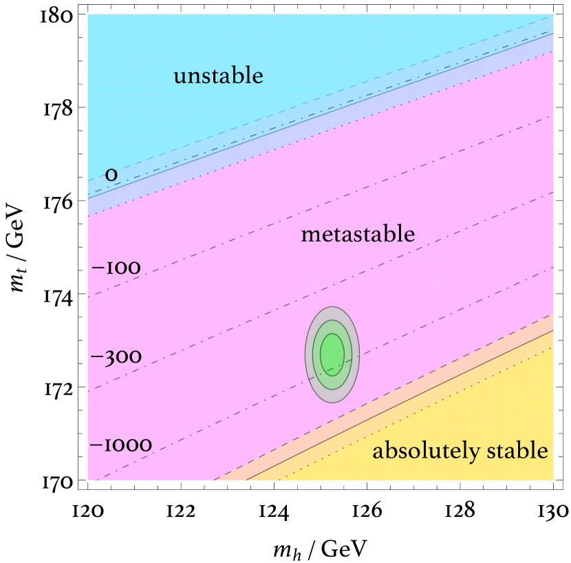
Figure 1: Contours of $\gamma$ as a function of the Higgs $m_{h}$ and the top mass $m_{t}$. The black dot-dashed contours correspond to $\gamma=1,10^{-100},10^{-300}$ and $10^{-1000}\text{ Gyr}^{-1}\text{Gpc}^{-3}$ for $\alpha_{s}(m_{Z})=0.1179$. In the blue region $\gamma$ becomes larger than $H_{0}^{4}$, with $H_{0}$ the current Hubble parameter, while in the yellow region the EW vacuum is stable. The boundaries of these regions are given by the plain lines for $\alpha_{s}(m_{Z})=0.1179$, the dotted lines for $\alpha_{s}(m_{Z})=0.1170$, the dashed line for $\alpha_{s}(m_{Z})=0.1188$. The green region, for which $\gamma=10^{-781}\text{ Gyr}^{-1}\text{Gpc}^{-3}$ at the center, shows the experimentally measured values of the Higgs and top masses with their $1\sigma$ (inside), $2\sigma$ (middle) and $3\sigma$ (outside) uncertainties in quadrature.

The stability of the EW vacuum has been investigated by several authors Sher (1989); Casas et al. (1995); Espinosa and Quiros (1995); Isidori et al. (2001); Espinosa et al. (2008); Ellis et al. (2009); Degrassi et al. (2012); Buttazzo et al. (2013); Lalak et al. (2014); Andreassen et al. (2014); Bednyakov et al. (2015); Branchina et al. (2015); Iacobellis and Masina (2016). The calculation of the full one-loop prefactor was first done in Isidori et al. (2001) before the Higgs discovery and updated in Andreassen et al. (2018); Chigusa et al. (2017, 2018) with a careful treatment of dilatation Andreassen et al. (2018); Chigusa et al. (2017, 2018) and gauge zero modes Endo et al. (2017a, b).

In this Letter we revisit the calculation of the gauge prefactor. We find that the transverse mode degeneracy was not properly taken into account. Once corrected, the central value of the SM rate $\gamma$ increases only slightly, from the previous $10^{-785}$ to $10^{-781}$ Gyr^-1 Gpc^-3. The SM vacuum lifetime remains longer than the current age of the universe and there is no occasion for anxiety Coleman (1977).

We first introduce the fluctuation operator in the gauge sector. Then we explain how to build suitable bases for the scalar and gauge fields, given the Euclidean spherical $4D$ symmetry of the bounce, and discuss the counting of degeneracy factors. Next, we obtain the analytic expression of our correction to the vacuum decay rate in the SM and give the numerical full one-loop vacuum decay rate with the current central values of the SM couplings. Our final result is summarized in FIG. 1.

Gauge fluctuation operator. In the presence of the bounce, gauge fields and NGBs mix. The fluctuation operator does not mix $Z_{\mu}$ and $W_{\mu}^{\pm}$ in the SM, so we unify the notation as $A_{\mu}=Z_{\mu},W_{\mu}^{\pm}$ and $\varphi=\varphi_{Z},\varphi^{\pm}$. The prefactor, coming from $A_{\mu}$ and $\varphi$, is then

$${\cal A}^{(A,\varphi)}=J_{G}\left(\frac{\det^{\prime}S^{\prime\prime(A,\varphi)}}{\det\hat{S}^{\prime\prime(A,\varphi)}}\right)^{-\frac{1}{2}}\,,$$ (2)

where the prime indicates the subtraction of the zero mode, associated with the spontaneous breaking of gauge symmetry, and $J_{G}$ is the group space integral Jacobian. The fluctuation operator in the $(A^{\mu},\varphi)$ basis is given by the $5\times 5$ matrix

$$\!\!\!S^{\prime\prime(A,\varphi)}=\begin{pmatrix}\left(-\partial^{2}+\frac{1}{4}g^{2}\overline{h}{}^{2}\right)\delta_{\mu\nu}&\frac{1}{2}g\overline{h}^{\prime}\hat{x}_{\nu}-\frac{1}{2}g\overline{h}\partial_{\nu}\\ g\overline{h}^{\prime}\hat{x}_{\mu}+\frac{1}{2}g\overline{h}\partial_{\mu}&-\partial^{2}+\lambda\overline{h}{}^{2}\end{pmatrix}\ ,$$ (3)

while $\hat{S}^{\prime\prime(A,\varphi)}$ is the same operator, but with $\bar{h}=0$. Here, $\bar{h}^{\prime}=\partial_{\rho}\bar{h}$, $g$ is the gauge coupling for $W^{\pm}$ or $Z$, and $\hat{x}_{\mu}$ is a unit vector, such that $x_{\mu}=\rho\,\hat{x}_{\mu}$. We work in the Fermi gauge with $\xi=1$, which is defined through the gauge fixing term $\mathcal{L}_{\rm GF}=(\partial_{\mu}A^{\mu})^{2}/2$. Given the $O(4)$ symmetry of the bounce, the 4$D$ Laplacian is conveniently written in spherical coordinates as $\partial^{2}=\partial_{\rho}^{2}+3\rho^{-1}\partial_{\rho}-L^{2}/\rho^{2}$, where $L^{2}=L^{\mu\nu}L_{\mu\nu}/2$, where $L_{\mu\nu}=-i(x_{\mu}\partial_{\nu}-x_{\nu}\partial_{\mu})$ is the orbital angular momentum operator.

The fluctuation operator commutes with rotations, and therefore with all the components of the total angular momentum operator, $[J_{\mu\nu},S^{\prime\prime(A,\varphi)}]=0$. This implies that only modes with the same total angular momentum quantum numbers mix under the action of (3). In the following we decompose $\varphi$ and $A_{\mu}$ into $J_{\mu\nu}$ bases. In the calculation of functional determinants, it is the total, not the orbital, angular momentum operator that dictates the counting of degeneracies.

Scalar field basis. The scalar field transforms under Euclidean rotations like $\varphi(x)\to\varphi(R^{-1}x)$, where $R$ is a finite rotation of coordinates. For the scalar, the total and orbital angular momenta coincide, $J_{\mu\nu}=L_{\mu\nu}$. The space of scalar fields carries an infinite dimensional unitary representation of the compact group $SO(4)$ that, thanks to the Peter-Weyl theorem, admits an orthogonal decomposition into irreducible finite dimensional representations (irreps). $SO(4)$ is locally isomorphic to $SU(2)_{A}\otimes SU(2)_{B}$. Following textbook conventions, in $SU(2)_{A}$ we define the total angular momentum operator in the $\hat{3}$ direction as $J_{A3}$ and the Casimir operator as $J_{A}^{2}$. The latter has eigenvalues $j_{A}(j_{A}+1)$ with $j_{A}$ a half-integer. The same holds for $SU(2)_{B}$ and we label the irreps with $(j_{A},j_{B})$, with dimension of $(2j_{A}+1)(2j_{B}+1)$.

The representation space of the scalar field splits into $\oplus_{j=0}^{\infty}(j/2,j/2)$, where the label $j=j_{A}+j_{B}$ is an integer. Each $(j/2,j/2)$ multiplet is an eigenstate of $J^{\mu\nu}J_{\mu\nu}/2=J^{2}=2(J_{A}^{2}+J_{B}^{2})$ with eigenvalue $j(j+2)$ and degeneracy factor $d_{j}^{(\varphi)}\equiv{\rm dim}\left(j/2,j/2\right)=\left(j+1\right)^{2}$.

An explicit basis for such irreps can be formed with hyperspherical harmonics $Y_{jm_{A}m_{B}}$ that satisfy $L^{2}Y_{jm_{A}m_{B}}=j(j+2)Y_{jm_{A}m_{B}}$. Here, $m_{A}$ and $m_{B}$ run in integer steps between $-j/2$ and $j/2$, giving the multiplicity $d_{j}^{(\varphi)}$. The NGB $\varphi$ is written as

$$\varphi(x)=\sum_{j=0}^{\infty}\sum_{m_{A},m_{B}}\varphi_{jm_{A}m_{B}}(\rho)\ Y_{jm_{A}m_{B}}(\hat{x})\,.$$ (4)

Vector field basis. For the spin-1 field, the total angular momentum is $J_{\mu\nu}=L_{\mu\nu}+S_{\mu\nu}$, where $[S_{\mu\nu}]_{\rho\sigma}=-i(\delta_{\mu\rho}\delta_{\nu\sigma}-\delta_{\mu\sigma}\delta_{\nu\rho})$ are the generators acting on the spin-component. The vector field transforms like $A_{\mu}(x)\to R_{\mu\nu}\,A_{\nu}(R^{-1}x)$, where $R_{\mu\nu}$ is the vector rotation matrix. The representation of $A_{\mu}(x)$ is isomorphic to the tensor product of a spin-1 component $(1/2,1/2)$, with an orbital component, transforming as $\oplus_{l=0}^{\infty}(l/2,l/2)$. To understand the $SO(4)$ irreps $(j_{A},j_{B})$ of the vector field, we expand the tensor product:

$$\begin{split}&\left(\frac{1}{2},\frac{1}{2}\right)\ \otimes\ \bigoplus_{l=0}^{\infty}\ \left(\frac{l}{2},\frac{l}{2}\right)=\\ &\hskip 4.30554pt\left(\frac{1}{2},\frac{1}{2}\right)\oplus\bigoplus_{l=1}^{\infty}\,\left[\left(\frac{l+1}{2},\frac{l+1}{2}\right)\oplus\left(\frac{l-1}{2},\frac{l-1}{2}\right)\right.\\ &\hskip 4.30554pt\left.\oplus\left(\frac{l+1}{2},\frac{l-1}{2}\right)\oplus\left(\frac{l-1}{2},\frac{l+1}{2}\right)\,\right]\,=\end{split}$$ (5)

$$\begin{split}&(0,0)_{l=1}\oplus\,\bigoplus_{j=1}^{\infty}\,\left[\left(\frac{j}{2},\frac{j}{2}\right)_{l=j+1}\oplus\left(\frac{j}{2},\frac{j}{2}\right)_{l=j-1}\right]\oplus\\ &\hskip 8.61108pt\bigoplus_{j=1}^{\infty}\,\left[\left(\frac{j+1}{2},\frac{j-1}{2}\right)_{l=j}\oplus\left(\frac{j-1}{2},\frac{j+1}{2}\right)_{l=j}\,\right]\,.\end{split}$$ (6)

Figure 2: Decomposition of a 4-vector field $A_{\mu}(\hat{x})$ under $SO(4)$. The diagonal modes ${\cal D}_{j}^{\pm}$ with $j_{A}=j_{B}$ appear in double copies, except for $(0,0)$. The off-diagonal multiplets with $j_{A}=j_{B}\pm 1$ correspond to the transverse modes ${\cal T}_{j}^{\pm}$, and appear as single copies. Blue circles with $l=3$ exemplify how the $L^{2}$ eigenspace gets distributed within the $(j_{A},j_{B})$ lattice.

To go from (5) to (6) we simply re-labeled and rearranged the sum. In (6) we included a subscript for each $(j_{A},j_{B})$ multiplet to track the orbital angular momentum quantum number $l$. We call the multiplets with $j_{A}=j_{B}$ the diagonal modes ${\cal D}^{\pm}_{j}$, corresponding to $(j/2,j/2)_{j\pm 1}$ (note ${\cal D}^{-}_{0}$ is zero); they have eigenvalue $j(j+2)$ under $J^{2}$, and degeneracy $d_{j}^{\cal D}\equiv{\rm dim}\left(\frac{j}{2},\frac{j}{2}\right)=\left(j+1\right)^{2}$. These are the same total angular momentum quantum numbers as the NGB scalars, hence the fluctuation operator matrix mixes these states. We identify the multiplets having $j_{A}=j_{B}\pm 1$ with the transverse modes Higuchi (1991), and call them ${\cal T}^{\pm}_{j}$ for $((j\pm 1)/2,(j\mp 1)/2)_{j}$. Their $J^{2}$ eigenvalue is $(j+1)^{2}$, while the degeneracy factor is

$$d_{j}^{\cal T} \equiv{\rm dim}\left(\frac{j\pm 1}{2},\frac{j\mp 1}{2}\right)=j\left(j+2\right)\,.$$ (7)

FIG. 2 summarizes the group theoretical construction and there ${\cal D}^{\pm}_{j}$ correspond to the diagonal circles, where the two overlapping circles are distinguished by the eigenvalues of $L^{2}$. The ${\cal T}^{\pm}_{j}$ correspond to the lower and upper off-diagonal circles, respectively.

We decompose $A_{\mu}(x)$ as a sum of radial functions times a basis of vector fields,

$$\!\!\!\!\!\!A_{\mu}(x)=\sum_{j_{A},j_{B},l,m_{A},m_{B}}A^{j_{A}j_{B}m_{A}m_{B}}_{l}(\rho)V^{j_{A}j_{B}m_{A}m_{B}}_{l;\mu}(\hat{x})\,,$$ (8)

where the real field $A_{\mu}$ is expanded with complex basis, without affecting the degeneracy, as follows

$$\begin{split}&V^{j_{A}j_{B}m_{A}m_{B}}_{l;\mu}(\hat{x})=\sum_{m_{l_{A}},m_{l_{B}},m_{s_{A}},m_{s_{B}}}C^{j_{A}m_{A}}_{\frac{l}{2}m_{l_{A}}\frac{1}{2}m_{s_{A}}}\\ &\hskip 8.61108ptC^{j_{B}m_{B}}_{\frac{l}{2}m_{l_{B}}\frac{1}{2}m_{s_{B}}}\left(\tilde{\sigma}_{\mu}\right)_{m_{s_{A}}m_{s_{B}}}\,Y_{lm_{l_{A}}m_{l_{B}}}(\hat{x})\,.\end{split}$$ (9)

This choice has the virtue of containing familiar objects that are in direct correspondence with the group theory construction of FIG. 2. The $(\tilde{\sigma}_{\mu})_{m_{s_{A}}m_{s_{B}}}$ matrices correspond to the $(1/2,1/2)$ object that ensures the proper transformation under rotations, and are given by $\tilde{\sigma}_{\mu}=\varepsilon\cdot\sigma_{\mu}$, where $\varepsilon$ is the two-dimensional Levi-Civita symbol, $\sigma_{1,2,3}$ are the usual Pauli matrices, and $\sigma_{4}=\text{diag}(i,i)$. The entries of $\tilde{\sigma}$ are ordered such that $m_{s}=1/2$ comes before $m_{s}=-1/2$. $C^{j_{A},m_{A}}_{l_{A}m_{l_{A}}s_{A}m_{s_{A}}}$ denote the $SU(2)_{A}$ Clebsch-Gordan coefficients (and the same for $B$). These are non-zero only when $|2j_{A,B}-l|=1$, $m_{A}=m_{l_{A}}+m_{s_{A}}$ and $m_{B}=m_{l_{B}}+m_{s_{B}}$. We shall suppress the $m$ indices from here on for brevity; they label the states with the same fluctuation operator and their summation only appears as the degeneracy factor. Then, the non-zero components of $V^{j_{A}j_{B}}_{l;\mu}$ are $V^{\frac{j}{2}\frac{j}{2}}_{l=j\pm 1;\mu}$ and $V^{\frac{j\pm 1}{2}\frac{j\mp 1}{2}}_{l=j;\mu}$, corresponding to the basis of ${\cal D}_{j}^{\pm}$ and ${\cal T}_{j}^{\pm}$. These components are eigenfunctions of $J^{2}$, with the eigenvalues quoted earlier for ${\cal D}_{j}^{\pm}$ and ${\cal T}_{j}^{\pm}$. Each component is an eigenfunction of $L^{2}$ that acts only on $Y_{lm_{l_{A}}m_{l_{B}}}$.

Fluctuation operator decomposition. Let us decompose (3) using the scalar and gauge basis functions in (4) and (8). When (3) acts on $(A_{\mu},\varphi)$, it splits into an infinite number of blocks with the same $j_{A},j_{B},m_{A}$ and $m_{B}$: $(A_{1}^{00},\varphi_{0})$ for $j=0$, and $(A_{j+1}^{\frac{j}{2}\frac{j}{2}},A_{j-1}^{\frac{j}{2}\frac{j}{2}},\varphi_{j})$, $(A_{j}^{\frac{j+1}{2}\frac{j-1}{2}})$, $(A_{j}^{\frac{j-1}{2}\frac{j+1}{2}})$ for $j>0$. The first two indicate $2\times 2$ or $3\times 3$ fluctuation matrices that mix the ${\cal D}^{\pm}_{j}$ modes with the NGB, and the last two are those for the ${\cal T}^{\pm}_{j}$ modes that do not mix.

With this decomposition, the prefactor in (2) factorizes into ${\cal A}^{(A,\varphi)}={\cal A}^{({\cal D},\varphi)}{\cal A}^{({\cal T})}$. The first term, ${\cal A}^{({\cal D},\varphi)}$, was already computed correctly in the previous literature Isidori et al. (2001); Andreassen et al. (2018); Chigusa et al. (2017). Therefore we only deal with the second one:

$${\cal A}^{({\cal T})}=\left[\prod_{j=1}^{\infty}\left(\frac{\det S^{\prime\prime({\cal T})}_{j}}{\det\hat{S}^{\prime\prime({\cal T})}_{j}}\right)^{2d_{j}^{\cal T}}\right]^{-\frac{1}{2}}\,.$$ (10)

The factor of $2$ in the exponent $2d_{j}^{\cal T}$ comes from the two transverse modes ${\cal T}^{\pm}_{j}$ having the same fluctuation operator, given by $S^{\prime\prime({\cal T})}_{j}=-\Delta_{j}+g^{2}\overline{h}{}^{2}/4$, where $\Delta_{j=l}=\partial_{\rho}^{2}+3\rho^{-1}\partial_{\rho}-l(l+2)\rho^{-2}$. There are no zero modes to worry about in (10), so there is no prime in the determinant at the numerator.

• In previous calculations Isidori et al. (2001); Andreassen et al. (2018); Chigusa et al. (2017), the degeneracy factor for the transverse modes, ${\cal T}_{j}^{\pm}$, was erroneously equal to $(j+1)^{2}$. The correct one, as we have shown in (7), is $d_{j}^{\cal T}=j(j+2)$. This leads to a slightly different result for the prefactor ${\cal A}^{(\cal T)}$. We will shortly revise that calculation.

• For the diagonal modes ${\cal D}^{\pm}_{j}$, our basis functions have one-to-one correspondence to the ones given in Isidori et al. (2001), which are then used in Andreassen et al. (2018); Chigusa et al. (2017, 2018). We differ for the transverse modes ${\cal T}^{\pm}_{j}$. In the supplemental material we show that their basis functions are linearly dependent and do not span the entire space. Despite the degeneracy factor and completeness issues, the operator $S^{\prime\prime({\cal T})}_{j}$ in Isidori et al. (2001); Andreassen et al. (2018); Chigusa et al. (2017) is correct.

• Ref. Isidori et al. (2001) stated that, if one works in the background gauge with $\xi=1$, i.e. $\mathcal{L}_{\rm GF}=(\partial_{\mu}A^{\mu}-g\bar{h}\varphi/2)^{2}/2$, the transverse and ghost modes mutually cancel. This is incorrect, given the corrected $d_{j}^{\cal T}$ in (7); one does need to include the ghost modes in this gauge.

Functional determinants for ${\cal T}^{\pm}$-modes. The infinite product in ${\cal A}^{({\cal T})}$ is ultraviolet divergent. A commonly employed regularization method subtracts the $\mathcal{O}(\delta S^{\prime\prime},\delta S^{\prime\prime 2})$ terms from $\ln{\cal A}^{(A,\varphi)}$, and adds back their dimensionally regularized quantities Isidori et al. (2001). Here, $\delta S^{\prime\prime}=S^{\prime\prime(A\varphi)}-\hat{S}^{\prime\prime(A\varphi)}$. The added-back terms do not suffer from the mode counting subtlety since they are calculated in momentum space. We focus on the subtraction procedure and defer to existing literature for the rest.

The finite part with the correct degeneracy factor is

$$\!\!\!\!\ln{\cal A}^{({\cal T})}_{\rm fin}=-\sum_{j=1}^{\infty}d_{j}^{\cal T}\left(\ln R_{j}-\ln R_{j}^{(1)}-\ln R_{j}^{(2)}\right)\,,$$ (11)

and it was finite even with the incorrect $d_{j}^{\cal T}$. The analytic formula Andreassen et al. (2018); Chigusa et al. (2018) for each term is

$$\ln R_{j}\equiv\ln\frac{\det S^{\prime\prime({\cal T})}_{j}}{\det\hat{S}^{\prime\prime({\cal T})}_{j}} =\ln\frac{\Gamma(j+1)\Gamma(j+2)}{\Gamma(j+\frac{3+\kappa}{2})\Gamma(j+\frac{3-\kappa}{2})}\,,$$ (12)

and

$$\ln R_{j}^{(1)} \equiv\left[\ln\frac{\det S^{\prime\prime({\cal T})}_{j}}{\det\hat{S}^{\prime\prime({\cal T})}_{j}}\right]_{\mathcal{O}(\delta S^{\prime\prime})}=\frac{g^{2}}{2|\lambda|}\frac{1}{j+1}\,,$$ (13)

$$\begin{split}\ln R_{j}^{(2)}&\equiv\left[\ln\frac{\det S^{\prime\prime({\cal T})}_{j}}{\det\hat{S}^{\prime\prime({\cal T})}_{j}}\right]_{\mathcal{O}(\delta S^{\prime\prime 2})}\\ &=\frac{g^{4}}{4\lambda^{2}}\left(\frac{2j+3}{2(j+1)^{2}}-\psi^{\prime}(j+1)\right)\,,\end{split}$$ (14)

with $\kappa=\sqrt{1-2g^{2}/|\lambda|}$ and $\psi(z)$ the digamma function.

As all the other fluctutations in the prefactor (1) were already computed correctly, we define the correction as

$$\delta\ln{\cal A}=\ln{\cal A}^{(A,\varphi)}_{\rm prev}-\ln{\cal A}^{(A,\varphi)},$$ (15)

where $\ln{\cal A}^{(A,\varphi)}_{\rm prev}$ is the gauge prefactor in Andreassen et al. (2018); Chigusa et al. (2018), and $\ln{\cal A}^{(A,\varphi)}$ the one computed with the correct degeneracy factor. We find

$$\begin{split}&\delta\ln{\cal A}=1-\frac{g^{4}}{16|\lambda|^{2}}(10-\pi^{2})-\frac{g^{2}}{2|\lambda|}(2-\gamma)\\ &\hskip 8.61108pt-\frac{5}{2}\ln 2\pi+\ln\left(\frac{4|\lambda|}{g^{2}}\cos\left(\frac{\pi}{2}\kappa\right)\right)\\ &\hskip 8.61108pt-\frac{1-\kappa}{2}\ln\Gamma\left(\frac{3-\kappa}{2}\right)-\frac{1+\kappa}{2}\ln\Gamma\left(\frac{3+\kappa}{2}\right)\\ &\hskip 8.61108pt+\psi^{(-2)}\left(\frac{3-\kappa}{2}\right)+\psi^{(-2)}\left(\frac{3+\kappa}{2}\right)\,.\end{split}$$ (16)

Vacuum decay rate. To compute the final updated decay rate, we rely on the analytic formulæ  for all the remaining prefactors calculated in Andreassen et al. (2018); Chigusa et al. (2018). We follow Chigusa et al. (2017, 2018) for the evaluation of the SM couplings at high energy. The gauge, top Yukawa, and Higgs quartic couplings at $\mu=m_{t}$ are determined using the fitting formulæ in Buttazzo et al. (2013), at NNLO precision. The bottom and tau Yukawa couplings are determined by $y_{b}(m_{b})=\sqrt{2}m_{b}(m_{b})/v$ and $y_{\tau}(m_{\tau})=\sqrt{2}m_{\tau}/v$. We ignore threshold corrections to bottom and tau masses; their effect on the vacuum decay rate is negligible. We run these couplings using the three-loop $\beta$-functions given in Buttazzo et al. (2013). The calculation of the rate involves an integral over the dilatation parameter $R$. The dilatation symmetry is broken by the running of the couplings and we include this effect by taking the renormalization scale to $\mu=1/R$, following Chigusa et al. (2017, 2018). We also put a UV cut-off to the integral such that $1/R$ or the maximum value of the Higgs field do not exceed the Planck scale Chigusa et al. (2018). The rate is then calculated using the public code ELVAS Chigusa et al. (2017, 2018), with the modification of the transverse mode degeneracy in the gauge sector.

We use the current values of the SM parameters and their $1\sigma$ errors from Workman et al. (2022): $m_{h}=125.25\pm 0.17\text{ GeV}$, $m_{t}=172.69\pm 0.30\text{ GeV}$ and $\alpha_{s}(m_{Z})=0.1179\pm 0.0009$. Our final decay rate is

$$\log_{10}\frac{\gamma}{\rm Gyr\,Gpc^{3}}=-781^{+45+154+180}_{-49-220-274}\,,$$ (17)

where the first, second, and third errors are calculated by changing the Higgs mass, the top mass, and the strong coupling by $1\sigma$, respectively. The variations are summarized in FIG. 1, which is similar to the one in the Addendum of Chigusa et al. (2017), where they used the same SM inputs.

Comparing to the most recent previous result Chigusa et al. (2017), we find $\gamma/\gamma_{\rm prev}\approx 10^{4}$, using the central values of the SM parameters. The change of the central value is much smaller than the uncertainties in (17). However, it is still larger than the theoretical uncertainty ($\approx 10^{3}$), evaluated by setting the renormalization scale to $\mu=2/R$ and $\mu=1/(2R)$ instead of $\mu=1/R$.

Summary. We revisited the total angular momentum decomposition of gauge fields in $4D$ and found an overcounting of degeneracies of the transverse modes gauge fluctuations in previous literature. We have recalculated the decay rate of the electroweak vacuum in the SM using the corrected counting, and found it increases a little. Even though the numerical difference compared to previous results is rather small, it is important to understand the conceptual issue with previous analyses and give a fully consistent picture of the meta-stability of the SM vacuum. The argument on the degeneracy factor applies to any calculation of gauge determinants in $4D$.

Acknowledgments. We wish to thank So Chigusa for providing a sample dataset for our numerical check. This work is supported by the Slovenian Research Agency under the research core funding No. P1-0035 and in part by the research grants N1-0253 and J1-4389.

Appendix A Previous vector field basis

In this section we examine the basis for the vector field first introduced in Isidori et al. (2001) and used in Chigusa et al. (2017, 2018); Andreassen et al. (2018). We write it as

$$\begin{split}A_{\mu}&=\sum_{j=0}^{\infty}\sum_{m_{A},m_{B}}\left(A^{(B)}_{jm_{A}m_{B}}(\rho)B^{jm_{A}m_{B}}_{\mu}(\hat{x})+A^{(L)}_{jm_{A}m_{B}}(\rho)L^{jm_{A}m_{B}}_{\mu}(\hat{x})\right.\\ &\quad\qquad\qquad\qquad\left.+A^{(T1)}_{jm_{A}m_{B}}(\rho)T^{1;jm_{A}m_{B}}_{\mu}(\hat{x})+A^{(T2)}_{jm_{A}m_{B}}(\rho)T^{2;jm_{A}m_{B}}_{\mu}(\hat{x})\right)\,,\end{split}$$ (18)

where $A^{(B,L,T1,T2)}_{jm_{A}m_{B}}(\rho)$ are the radial parts, functions of the Euclidean radius $\rho$ only. Here, the labels $j,m_{A}$ and $m_{B}$ correspond to the labels $j,m$ and $m^{\prime}$ introduced in Isidori et al. (2001), which indicate the hyperspherical harmonics that the basis functions are constructed from. The orbital parts do not depend on $\rho$ and are only functions of $\hat{x}$, or the three angles in 4D. We separate them into $B$ modes, proportional to the ‘breathing’ direction $\hat{x}_{\mu}$, and longitudinal-like $L$ modes along the momentum $\rho\partial_{\mu}$:

$$B^{jm_{A}m_{B}}_{\mu}(\hat{x}) =\hat{x}_{\mu}\,Y_{jm_{A}m_{B}}(\hat{x})\,, L^{jm_{A}m_{B}}_{\mu}(\hat{x}) =\rho\partial_{\mu}\,Y_{jm_{A}m_{B}}(\hat{x})\,.$$ (19)

Orthogonally to these two, the authors of Isidori et al. (2001) defined the transverse modes,

$$T^{i;jm_{A}m_{B}}_{\mu}(\hat{x}) =i\epsilon_{\mu\nu\rho\sigma}V^{(i)}_{\nu}L_{\rho\sigma}Y_{jm_{A}m_{B}}(\hat{x})\,, i =1,2\,,$$ (20)

where $V^{(1)}_{\mu}$ and $V^{(2)}_{\mu}$ are two arbitrary independent vectors. The construction relies on the hyperspherical harmonics that we label as $Y_{jm_{A}m_{B}}$. They are eigenfunctions of the $L^{2}$ operator, $L^{2}Y_{jm_{A}m_{B}}=j(j+2)Y_{jm_{A}m_{B}}$, where the label $j$ is an integer, while $m_{A}$ and $m_{B}$ range between $-j/2$ and $j/2$ in integer steps, giving the multiplicity $(j+1)^{2}$. Naïvely, it looks like each set of functions, $B,L,T^{1},T^{2}$, spans a space with dimension $(j+1)^{2}$ for any $j>0$, which is what was assumed in Isidori et al. (2001); Chigusa et al. (2017, 2018); Andreassen et al. (2018). We will show that this is not the case.

In particular, the transverse modes $T^{1}$ and $T^{2}$ only cover a space with dimension $2j(j+2)-j$ for any $j>0$. This is neither equal to the naïve $2(j+1)^{2}$, nor to the correct $2j(j+2)$, which we will obtain with group theoretical arguments. Thus, the basis functions in (18) have to be dependent and incomplete. Let us start with the $B$ and $L$ modes, which are orthogonal to each other. The $j=0$ mode is constructed from $Y_{000}(\hat{x})=1/\sqrt{4\pi}$. Therefore, only $B_{\mu}^{000}$ is non zero, while $L_{\mu}^{000}$ and $T^{i;000}_{\mu}$ vanish because they contain a derivative hitting the constant $Y_{000}$. Also, $B_{\mu}^{000}$ is proportional to $V^{00}_{l=1;\mu}$ [see (9)], which corresponds to the singlet state with $j=0$. Next, consider $j\geq 1$. Both $B^{jm_{A}m_{B}}_{\mu}$ and $L^{jm_{A}m_{B}}_{\mu}$ are non-zero for all $m_{A}$ and $m_{B}$. Note that the $\hat{x}^{\mu}$ and $\partial_{\mu}$ operators commute with $J_{\mu\nu}$. This implies that $B^{jm_{A}m_{B}}_{\mu}$ and $L^{jm_{A}m_{B}}_{\mu}$ have the total angular momentum quantum numbers $j_{A}=j_{B}=j/2$, and are orthogonal to each other. They are eigenfunctions of $J^{2}$ with eigenvalue $j(j+2)$, and have the same degeneracy factor as the hyperspherical harmonics, $(j+1)^{2}$.

Another way of understanding the degeneracy is to calculate the number of independent functions from the rank of the Gram matrix formed from the basis functions. We have

$$d_{j}^{B} =\operatorname{Rank}\left(\sum_{\mu}\int{\rm d}\Omega(B^{jm_{A}m_{B}}_{\mu})^{*}B^{jm^{\prime}_{A}m^{\prime}_{B}}_{\mu}\right)=\operatorname{Rank}\left(\delta_{m_{A}m^{\prime}_{A}}\delta_{m_{B}m^{\prime}_{B}}\right)=\left(j+1\right)^{2}\,,$$ (21)

where we plugged in the definition of $B^{jm_{A}m_{B}}_{\mu}$ and used the fact that $\sum_{\mu}\hat{x}_{\mu}^{2}=1$. This reduces the integral to the usual statement of spherical harmonic orthonormality after integrating over $\int{\rm d}\Omega$. We also merged $m_{A}$ and $m_{B}$ into a single index and the Gram matrix becomes a $(j+1)^{2}\times(j+1)^{2}$ matrix. A similar calculation goes through for the longitudinal-like modes, where we integrate by parts and express the Cartesian second derivative in the spherical basis as $\Delta_{l}$. The radial derivatives vanish when we act on $\partial_{\rho}^{n}((B,L)(\hat{x}))=0$ and only the orbital momentum operator $L^{2}/\rho^{2}$ part remains, such that

$$d_{j}^{L} =\operatorname{Rank}\left(\sum_{\mu}\int{\rm d}\Omega(L^{jm_{A}m_{B}}_{\mu})^{*}L^{jm^{\prime}_{A}m^{\prime}_{B}}_{\mu}\right)=\operatorname{Rank}\left(j(j+2)\delta_{m_{A}m^{\prime}_{A}}\delta_{m_{B}m^{\prime}_{B}}\right)=\begin{cases}0\,,&j=0\,,\\ (j+1)^{2}\,,&j>0\,.\end{cases}$$ (22)

The $L^{2}$ eigenvalue of $Y_{jm_{A}m_{B}}$ is simply $j(j+2)$ and is just a number that does not affect the rank for $j>0$; it only takes care of removing the $j=0$ mode. As expected, the Gram matrix for generic $j>0$ is full-rank, except for $L_{\mu}^{000}$ that vanishes.

We have recovered the result of the group theoretical argument in the main text. It follows that the modes $B^{jm_{A}m_{B}}_{\mu}$ and $L^{jm_{A}m_{B}}_{\mu}$ cover exactly the same space spanned by our ${\cal D}_{j}^{\pm}$ basis, which is a $2(j+1)^{2}$ dimensional space. Unlike $V^{j_{A}j_{B}}_{l;\mu}$, the $B^{jm_{A}m_{B}}_{\mu}$ and $L^{jm_{A}m_{B}}_{\mu}$ are still not eigenstates of $L^{2}$ and it is diagonalized by taking linear combinations,

$$V^{\frac{j}{2}\frac{j}{2}m_{A}m_{B}}_{l=j+1;\mu} \propto\left(j+2\right)\,B^{jm_{A}m_{B}}_{\mu}-L^{jm_{A}m_{B}}_{\mu}\,, V^{\frac{j}{2}\frac{j}{2}m_{A}m_{B}}_{l=j-1;\mu} \propto j\,B^{jm_{A}m_{B}}_{\mu}+L^{jm_{A}m_{B}}_{\mu}\,,$$ (23)

where the first function corresponds to the ${\cal D}_{j}^{+}$ multiplet and the second to ${\cal D}_{j}^{-}$. The degeneracy factor for these modes was treated correctly in previous literature. Let us then turn to the transverse modes, for which the situation is more involved.

Appendix B Transverse gauge modes

First note that the $T^{i;jm_{A}m_{B}}_{\mu}$ are not eigenstates of $J_{A3,B3}$, the third component of the $SU(2)_{A}$ and $SU(2)_{B}$ total angular momentum. Hence, the labels $m_{A}$ and $m_{B}$ do not correspond to the eigenvalues of $J_{A3}$ and $J_{B3}$, they are just inherited from the labels of spherical harmonics. Thus having different $m_{A}$ and $m_{B}$ does not ensure that the functions are independent. The $J^{2}$ eigenvalue for $T^{i;jm_{A}m_{B}}_{\mu}$ is given by $(j+1)^{2}$, therefore they have to be related to the ${\cal T}^{\pm}_{j}$ modes. However, we know from the discussion in the main text that there exist only $2j(j+2)$ independent basis functions for ${\cal T}^{\pm}_{j}$. Let us then analyze the space spanned by $T^{1,2;jm_{A}m_{B}}_{\mu}$.

Computing the degeneracy of $T^{1}$. We invoke again the rank of the Gram matrix. First, though, we need some preliminaries. Without loss of generality we take $V^{(1)}_{\mu}=\delta_{\mu 4}$ and $V^{(2)}_{\mu}=\delta_{\mu 3}$ as the two independent vectors in (20). Then we define the $SU(2)_{A}$ and $SU(2)_{B}$ orbital angular momentum operators as

$$L_{Ai} =\frac{1}{4}\left(\epsilon_{ijk}L_{jk}+2L_{4i}\right)\,, L_{Bi} =\frac{1}{4}\left(\epsilon_{ijk}L_{jk}-2L_{4i}\right)\,.$$ (24)

They are normalized such that they satisfy the canonical $SU(2)_{A,B}$ algebras $[L_{Ai},L_{Aj}]=i\epsilon_{ijk}L_{Ak}$, $[L_{Bi},L_{Bj}]=i\epsilon_{ijk}L_{Bk}$ and commute with one another $[L_{Ai},L_{Bj}]=0$. Then we have

$$d_{j}^{(T1)} =\operatorname{Rank}\left(\sum_{\mu}\int{\rm d}\Omega\,(T^{1;jm_{A}m_{B}}_{\mu})^{*}T^{1;jm^{\prime}_{A}m^{\prime}_{B}}_{\mu}\right)=\operatorname{Rank}\left(\int{\rm d}\Omega\,Y^{*}_{jm_{A}m_{B}}4\sum_{i}\left(L_{Ai}+L_{Bi}\right)^{2}Y_{jm^{\prime}_{A}m^{\prime}_{B}}\right)\,.$$ (25)

Let us evaluate the action of the $L_{Ai}+L_{Bi}=L_{Ci}$ operator on spherical harmonics in (25). Because $A$ and $B$ sectors commute, the $C$ operators themselves form an $SU(2)_{C}$ algebra that represents a simultaneous rotation in both $SU(2)_{A,B}$ spaces. Its states can be labeled by $l_{C}$ that ranges from $|l_{A}-l_{B}|\leq l_{C}\leq l_{A}+l_{B}$. The hyperspherical harmonics $Y_{jm_{A}m_{B}}$ correspond to $(j/2,j/2)=(l_{A},l_{B})$. Because $l_{A}=l_{B}$, the minimal value of $l_{C}$ is always $0$ for each fixed $j$ in (25). The eigenvalue of the Casimir operator $L_{C}^{2}=\sum_{i}\left(L_{Ai}+L_{Bi}\right)^{2}$ is in general given by $l_{C}(l_{C}+1)$ (as for the canonical $SU(2)_{C}$) and therefore vanishes for $l_{C}=0$. This means that there will always be a single zero eigenvalue in the Gram matrix of $T^{1}$, the rest are non-zero. Without the zero, the matrix would be full rank with the degeneracy of $(j+1)^{2}$, because none of the states would be lost in the last equality of (25). However, the zero is present for each $j$ (this is in contrast to (22), where the zero is there only for $j=0$) and therefore reduces $d_{j}^{(T1)}$ by 1 and we have

$$d_{j}^{(T1)}=\left(j+1\right)^{2}-1=j\left(j+2\right)\,.$$ (26)

The vanishing linear combination among the $T^{1}$ modes, whose existence is guaranteed by the previous arguments and which corresponds to the singlet of $L_{C}$, is given explicitly by

$$0=\sum_{m=-j/2}^{j/2}(-1)^{m}\,T^{1;jm(-m)}_{\mu}\,.$$ (27)

Had we started with a different choice of $V^{(i)}_{\mu}$, by rotational symmetry of the problem we would have obtained the same result, therefore $d_{j}^{(T2)}=j\left(j+2\right)$. Furthermore, in analogy to (27), there is a vanishing linear combination among the $T^{2}$ modes, given explicitly as $0=\sum_{m=-j/2}^{j/2}T^{2;jm(-m)}_{\mu}$.

With the calculated $d_{j}^{(T1,T2)}$ it looks like we got exactly what was expected from group theoretical grounds. It appears that the calculation of the transverse mode determinant, using the basis proposed in Isidori et al. (2001), would be perfectly fine, if only the correct degeneracy factor were used. However, this is not the end of the story, as it turns out that $T^{1}$ and $T^{2}$ have an overlapping space, as we are going to show.

Additional overlaps among $T^{1,2}$ transverse modes. We want to prove here that the transverse modes $T^{1,2}$, defined in (20), do not span the whole $2j(j+2)$ dimensional space of transverse fluctuations. Specifically, at each $j$ we find that precisely $j$ modes are linearly dependent, such that

$$d_{j}^{(T1\cup T2)}=d_{j}^{(T1)}+d_{j}^{(T2)}-j=j(2j+3)\,,$$ (28)

where we called $d_{j}^{(T1\cup T2)}$ the dimension of the space generated by (20) at a given $j$.

To better understand the nature of the problem, it is useful to split the $T^{1,2}$ modes into those having $m_{A}+m_{B}\neq 0$ and those having $m_{A}+m_{B}=0$. The first class is made of $j(j+1)$ $T^{1}$ modes and $j(j+1)$ $T^{2}$ modes, while the second class is made of $j$ $T^{1}$ modes and $j$ $T^{2}$ modes. The reason why there are only $j$ modes in the second class, and not $j+1$, is due to (27) and its homologous for $T^{2}$ modes. Notice in fact that the vanishing linear combinations only involve modes of the form $T^{i;jm(-m)}$. Due to the Gram determinant discussion, resulted in (26), we also know that there is no other vanishing linear combination within the set of $T^{1}$ modes, and in particular all those $j(j+1)$ modes with $m_{A}+m_{B}\neq 0$ are linearly independent. The same holds for $T^{2}$. However we cannot say much, for the moment, about possible linear relations among the combined set comprising both $T^{1}$ and $T^{2}$ modes. This is what we are going to investigate next.

Firstly, we are going to prove that all $T^{1}$ and $T^{2}$ modes belonging to the first class (with $m_{A}+m_{B}\neq 0$) are linearly independent. With a little bit of algebra it can be shown that the $T^{1,2}$ modes take on the following form

$$T^{1;jm_{A}m_{B}}_{\mu} \propto\begin{pmatrix}*\\ *\\ m_{A}+m_{B}\\ 0\end{pmatrix}Y_{jm_{A}m_{B}}\,, T^{2;jm_{A}m_{B}}_{\mu} \propto\begin{pmatrix}*\\ *\\ 0\\ m_{A}+m_{B}\\ \end{pmatrix}Y_{jm_{A}m_{B}}\,,$$ (29)

where $*$ indicates some linear combinations of $L_{\mu\nu}$. Thanks to the linear independence of the spherical harmonics and the fact that $m_{A}+m_{B}\neq 0$, it follows that all modes belonging to the first class are independent, which means that they span altogether a $2j(j+1)$-dimensional space. For what concerns modes with $m_{A}+m_{B}=0$, which have only zeroes in the last two components, by inspection of (29) we can also conclude that they generate a subspace which is linearly independent from the one generated by the modes with $m_{A}+m_{B}\neq 0$. What is the dimension of this subspace is our next question.

With a little bit of algebra, we find

$$T^{1;jm(-m)}_{\mu} =\begin{pmatrix}i(L_{A+}+L_{A-}+L_{B+}+L_{B-})\\ L_{A+}-L_{A-}+L_{B+}-L_{B-}\\ 0\\ 0\end{pmatrix}Y_{jm(-m)}\,,$$ (30)

$$T^{2;jm(-m)}_{\mu} =\begin{pmatrix}L_{A+}-L_{A-}-L_{B+}+L_{B-}\\ i(-L_{A+}-L_{A-}+L_{B+}+L_{B-})\\ 0\\ 0\end{pmatrix}Y_{jm(-m)}\,,$$ (31)

where the orbital ladder operators are defined in the usual way as $L_{A\pm}=L_{A1}\pm iL_{A2}$ and $L_{B\pm}=L_{B1}\pm iL_{B2}$. Working out the action of the ladder operators on the spherical harmonics, one finds that the nonzero components of $T^{1,2}$ have the following form

$$T^{1;jm(-m)}_{\mu} =\begin{pmatrix}i(P_{m}+P_{m-1})\\ Q_{m}+Q_{m-1}\end{pmatrix}\,, T^{2;jm(-m)}_{\mu} =\begin{pmatrix}P_{m}-P_{m-1}\\ -i(Q_{m}-Q_{m-1})\end{pmatrix}\,,$$ (32)

where, at a given $j$,

$$P_{m},Q_{m} =\sqrt{\left(\frac{j}{2}+m+1\right)\left(\frac{j}{2}-m\right)}\left(Y_{j(m+1)(-m)}\,\pm\,Y_{jm(-m-1)}\right)\,.$$ (33)

By inspection of the second expression of (32), knowing that $P_{-\frac{j}{2}-1},Q_{-\frac{j}{2}-1}=0$, we find that

$$i\sum_{\sigma=-\frac{j}{2}}^{m}T^{2;j\sigma(-\sigma)}_{\mu}=\begin{pmatrix}iP_{m}\\ Q_{m}\end{pmatrix}$$ (34)

(a completely analogous expression can be obtained by taking an alternate sum over $T^{1}$ modes). Eq. (34) allows to derive the following set of $j+1$ identities, expressing $T^{1;jm(-m)}_{\mu}$ modes as a linear combination of $T^{2;jm(-m)}_{\mu}$ modes

$$T^{1;jm(-m)}_{\mu}=i\sum_{\sigma=-\frac{j}{2}}^{m}T^{2;j\sigma(-\sigma)}_{\mu}+i\sum_{\sigma=-\frac{j}{2}}^{m-1}T^{2;j\sigma(-\sigma)}_{\mu}\,.$$ (35)

Let us explain why this equality allows to conclude that Eq. (28) holds. We know for sure from the Gram determinant discussion that there are exactly $j$ independent $T^{2}$ modes of the form $T^{2;jm(-m)}$, which are also independent from all modes with $m_{A}+m_{B}\neq 0$, as we just showed. Eq. (35) shows that all $T^{1}$ modes of the form $T^{1;jm(-m)}$ are linearly dependent (on the $T^{2;jm(-m)}$ modes). Even though we declare $j+1$ linear identities, exactly one of them is redundant, because of (27).

Summarizing, we have found that there are $2j(j+1)$ independent modes having $m_{A}+m_{B}\neq 0$, and that out of the initial $2j$ modes having $m_{A}+m_{B}=0$, which a span an independent space on their own, only $j$ are independent (say the $T^{2}$ modes). All in all we have $d_{j}^{(T1\cup T2)}=2j\left(j+1\right)+j=j\left(2j+3\right)$, as we wanted to show.

Our proof was built on making the choice $V^{(1)}=\delta_{\mu 4},V^{(2)}=\delta_{\mu 3}$. These two directions play a special role: the first in defining “boosts”, the second in picking up a quantization axis. Rotational invariance of the problem guarantees that any choice of two orthogonal vectors would lead to the same conclusion. Indeed, any two orthogonal vectors can be rotated to $\delta_{\mu 4}$ and $\delta_{\mu 3}$.

Completing the transverse basis. The missing $j$ transverse modes can be chosen as

$$T^{3;j(m-1)(-m)}_{\mu} V_{\nu}^{(3)} =\delta_{\nu 1}+i\delta_{\nu 2}\,.$$ with (36)

We see indeed that the fourth component of $T^{3;j(m-1)(-m)}_{\mu}$ is

$$T^{3;j(m-1)(-m)}_{\mu=4}=-2i\sqrt{\left(\frac{j}{2}+m\right)\left(\frac{j}{2}+1\right)}Y_{jm(-m)}-2i\sqrt{\left(\frac{j}{2}-m+1\right)\left(\frac{j}{2}+m\right)}Y_{j(m-1)(-m+1)}\,,$$ (37)

which is independent from $T^{1,2}_{\mu=4}$ because it contains the missing $Y_{jm(-m)}$. Independence of the fourth component implies independence of the $j$ vectors in (36) from the previously considered vectors. Now, $T^{2;jm_{A}m_{B}}$ with arbitrary $m_{A,B}$ modulo the singlet removal (in total $j(j+2)$ modes), $T^{1;jm_{A}m_{B}}$ with $m_{A}+m_{B}\neq 0$ (in total $j(j+1)$ modes) and $T^{3;j(m-1)(-m)}$ (in total $j$ modes) are independent and correctly span the whole $2j(j+2)$ dimensional space of transverse fluctuations.

Appendix C Canonical basis of transverse modes

An alternative to the basis given in the previous section, one that elaborates on the ansatz of Isidori et al. (2001), Eq. (20), is given by the following expression

$$T^{\pm;jm_{A}m_{B}}_{\mu}(\hat{x})=\sum_{m_{l_{A}},m_{l_{B}}}\epsilon_{\mu\nu\rho\sigma}\left({\bf V}^{\pm}_{\nu}\right)^{m_{A}\ m_{B}}_{m_{l_{A}}m_{l_{B}}}L_{\rho\sigma}Y_{jm_{l_{A}}m_{l_{B}}}(\hat{x})\,,$$ (38)

where the matrix-valued 4-vector ${\bf V}_{\nu}^{\pm}$, converting the $(j/2,j/2)$ indices of the spherical harmonics to $((j\pm 1)/2,(j\mp 1)/2)$ indices (the ones appropriate for the transverse modes, as discussed in the main text), is given in terms of Clebsch-Gordan coefficients as

$$\left({\bf V}^{\pm}_{\nu}\right)^{m_{A}\ m_{B}}_{m_{l_{A}}m_{l_{B}}}=\sum_{m_{s_{A}},m_{s_{B}}}C^{\frac{j\pm 1}{2}m_{A}}_{\frac{j}{2}m_{l_{A}}\frac{1}{2}m_{s_{A}}}C^{\frac{j\mp 1}{2}m_{B}}_{\frac{j}{2}m_{l_{B}}\frac{1}{2}m_{s_{B}}}\left(\tilde{\sigma}_{\nu}\right)_{m_{s_{A}}m_{s_{B}}}\,,$$ (39)

with $\tilde{\sigma}_{\nu}$ as in (9). Eq. (38) is nothing but a linear combination of objects of the form of (20). The virtue of this specific linear combination is that the $m_{A,B}$ indices now do correspond to the eigenvalues of the $J_{A3}$ and $J_{B3}$ operators, making (38) a canonical multiplet of $SO(4)\simeq SU(2)\times SU(2)$. Moreover, the ansatz of Isidori et al. (2001) makes transversality of the modes manifest.

Let us comment on the mechanics behind (38). The main observation is that, under a rotation acting on the vector field $T^{\pm}_{\mu}(\hat{x})$, it can be shown that the combination $\epsilon_{\mu\nu\rho\sigma}(\tilde{\sigma}_{\nu})_{m_{s_{A}}m_{s_{B}}}L_{\rho\sigma}Y_{jm_{l_{A}}m_{l_{B}}}(\hat{x})$ transforms as the tensor product $(j/2,j/2)\otimes(1/2,1/2)$, where the first and second factor act respectively on the indices $m_{l_{A}},m_{l_{B}}$ and $m_{s_{A}},m_{s_{B}}$. In order to project on the $((j\pm 1)/2,(j\mp 1)/2)$ subrepresentations, the ones characterizing transverse modes, we contract with $C^{\frac{j\pm 1}{2}}C^{\frac{j\mp 1}{2}}$. This is completely analogous to the standard procedure with the rotation group $SO(3)$, with the difference here that there are two factors of $SO(3)\simeq SU(2)$, so we need to multiply by two Clebsch-Gordan coefficients. As a cross check of the consistency of the method, it can be verified that contracting with $C^{\frac{j+1}{2}}C^{\frac{j+1}{2}}$ or with $C^{\frac{j-1}{2}}C^{\frac{j-1}{2}}$ gives zero, because diagonal modes are already projected out by the $\epsilon_{\mu\nu\rho\sigma}$. The modes of (38) are proportional to the ${\cal T}^{\pm}$ modes presented in the main text.

Appendix D Counting in orbital modes

Another possible basis for the vector field is

$$A_{\mu}(x)=\sum_{l,m_{l_{A}},m_{l_{B}}}\left(\delta_{\mu 1}A_{lm_{l_{A}}m_{l_{B}}}^{(1)}(\rho)+\delta_{\mu 2}A_{lm_{l_{A}}m_{l_{B}}}^{(2)}(\rho)+\delta_{\mu 3}A_{lm_{l_{A}}m_{l_{B}}}^{(3)}(\rho)+\delta_{\mu 4}A_{lm_{l_{A}}m_{l_{B}}}^{(4)}(\rho)\right)Y_{lm_{l_{A}}m_{l_{B}}}(\hat{x})\,.$$ (40)

Here we use the label $l$ to emphasize that the hyperspherical harmonics are eigenfunctions of $L^{2}$, the Casimir of the orbital angular momentum operator. The form (40) makes it obvious that the vector can be seen as a collection of four scalar degrees of freedom. As such, for each $l$ the vector has degeneracy of $4(l+1)^{2}$. Let us count the degeneracies in terms of the orbital angular momentum quantum number $l$ for the basis we introduced in the main text, and for the $B,L,T^{i}$ basis we discussed just above.

We saw that the transverse modes in either basis, ${\cal T}_{j}^{\pm}$ or $T^{i=1,2,3}_{\mu}$, have $l=j$. Their degeneracy is $2l(l+2)=2j(j+2)$. The other two modes with $l=j$ are

$$V^{\frac{j+1}{2}\frac{j+1}{2}}_{l=j;\mu}\propto\left(l+1\right)B^{(l+1)m_{A}m_{B}}_{\mu}+L^{(l+1)m_{A}m_{B}}_{\mu}\in\left(\frac{l+1}{2},\frac{l+1}{2}\right)_{l=j}\,,$$ (41)

$$V^{\frac{j-1}{2}\frac{j-1}{2}}_{l=j;\mu}\propto\left(l+1\right)B^{(l-1)m_{A}m_{B}}_{\mu}-L^{(l-1)m_{A}m_{B}}_{\mu}\in\left(\frac{l-1}{2},\frac{l-1}{2}\right)_{l=j}\,,$$ (42)

which have $(l+2)^{2}$ and $l^{2}$ degeneracies, respectively. Summing all of them up, we have

$$\left(l+2\right)^{2}+l^{2}+2l\left(l+2\right)=4\left(l+1\right)^{2}\,,$$ (43)

which is consistent with that of four scalars, as expected.

The basis (40) looks much simpler than the one we adopted in the main text or the one introduced in Isidori et al. (2001). However, its modes are not eigenfunctions of the total angular momentum operators ($J_{A}^{2},J_{B}^{2},J_{A3},J_{B3}$). As we stressed in the main text, the fluctuation operator (3), which acts on the $(A_{\mu},\varphi)$ basis, always commutes with $J_{\mu\nu}$, but in general not with $L_{\mu\nu}$ and $S_{\mu\nu}$ separately. In order to take advantage of symmetries to diagonalize the fluctuation operator, it is therefore much more convenient to use a basis for $A_{\mu}$ like the one we chose in this work, or the one chosen in Isidori et al. (2001).