DVOS: Self-Supervised Dense-Pattern Video Object Segmentation

Abstract

Video object segmentation approaches primarily rely on large-scale pixel-accurate human-annotated datasets for model development. In Dense Video Object Segmentation (DVOS) scenarios, each video frame encompasses hundreds of small, dense, and partially occluded objects. Accordingly, the labor-intensive manual annotation of even a single frame often takes hours, which hinders the development of DVOS for many applications. Furthermore, in videos with dense patterns, following a large number of objects that move in different directions poses additional challenges. To address these challenges, we proposed a semi-self-supervised spatiotemporal approach for DVOS utilizing a diffusion-based method through multi-task learning. Emulating real videos’ optical flow and simulating their motion, we developed a methodology to synthesize computationally annotated videos that can be used for training DVOS models; The model performance was further improved by utilizing weakly labeled (computationally generated but imprecise) data. To demonstrate the utility and efficacy of the proposed approach, we developed DVOS models for wheat head segmentation of handheld and drone-captured videos, capturing wheat crops in fields of different locations across various growth stages, spanning from heading to maturity. Despite using only a few manually annotated video frames, the proposed approach yielded high-performing models, achieving a Dice score of $0.82$ when tested on a drone-captured external test set. While we showed the efficacy of the proposed approach for wheat head segmentation, its application can be extended to other crops or DVOS in other domains, such as crowd analysis or microscopic image analysis.

1 Introduction

Deep learning (DL) techniques are widely used for analyzing visual data, such as images and videos. Developing advanced methods for comprehending visual data enhances the efficiency and speed of various tasks involving visual data processing across various computerized tasks [51, 29, 5, 47], specifically video-based models that benefit from videos’ spatial and temporal forms of information. Video object segmentation (VOS) is a critical computer vision task that tackles the challenge of automatically extracting and precisely outlining objects of interest at the pixel level across consecutive frames in a video sequence. In VOS, the association between pixels and objects can change over time as the object or camera moves. Videos, in contrast to static images, encapsulate the dynamic scope of motion and interaction unfold over time. This temporal information can be utilized for DL analysis. Nevertheless, videos constantly exhibit high levels of noise, influenced by natural factors in uncontrollable environments, such as camera movement and specifications, wind, and suboptimal illumination such as bright sunlight. Videos in agriculture contexts often represent these characteristics.

Developing high-performing DL models, either for image- or vide-based models, is not a trivial task and faces several challenges, such as data annotation bottlenecks [46, 16, 29] and designing or choosing suitable DL architectures, considering the available data and computational resources as well as the complexity of task at hand [51, 22, 43]. Most efforts on utilizing DL for visual data processing have been focused on supervised learning approaches, where large-scale annotated datasets are needed for developing these models. The resource-intensive nature of data annotation has hindered the full utilization of DL-based image processing approaches for many tasks that need pixel-level annotations. This issue is more pronounced for VOS tasks. To represent continuous and smooth motion, a single video file may contain thousands of video frames, where each video frame is a single image  [21]. As such, manual annotation of videos is a highly laborious and expensive process, rendering the use of supervised learning approaches impractical for many tasks requiring object-level and pixel-level data annotation [36, 32]. Annotating videos become even more resource-intensive when they involve a large number of objects, a common scenario is precision agriculture [28, 29], where the agricultural field images usually contain many densely located plants, resulting in a large number of objects of interest—such as leaves, stems, flowers, and spikes—in each image.

Despite the substantial challenges in developing large-scale annotated datasets, particularly for VOS, videos are generally considered more suitable for segmentation, compared to static image frames. Videos can help identify partial occlusions, as analysis of video frames independently presents transient artifacts. These artifacts could be overcome by analyzing a sequence of frames. Furthermore, analyzing video frames independently results in information loss regarding objects’ movement and deformation. Independent single-frame analysis also fails to deal with visual artifacts such as background clutter and transient objects, which complicates the segmentation of an object within consecutive frames. For instance, the shadow of moving wheat heads in windy environments on the ground can cause a one-frame transient objects artifact that adversely affects the accuracy of the single-frame object segmentation models. The temporal information within videos can serve as a crucial differentiator, enabling video-based models to accurately follow object movement and deformations in the presence of the artifacts [20, 30]. This capability is indispensable for tasks involving the segmentation of objects undergoing dynamic appearance changes. Examples include crops swaying in the wind, moving animals, and crowd analysis.

While the state-of-the-art VOS approaches commonly opt to compute temporal matching in the form of optical flow and dense trajectories [38, 5, 55], others prefer the parallel strategy that process frames independently [33, 25]. These studies rely on the availability of large-scale annotated datasets, i.e., the pixel-level annotation for each target object in every video frame, to serve as the primary input for training DL models [38, 18, 5, 55]. Also, It has been reported that for general-purpose tasks involving one or two large target objects, these models often take shortcuts by predicting subsequent masks solely based on the provided preceding frame’s mask, thereby bypassing the rich information offered by the preceding frames themselves [55]. This oversight led to shortcomings in the predicted segmentation maps, stemming from obscured objects in earlier frames and missed objects within the most recent mask [25].

Video data, using either spatial or temporal information, has found widespread applications in precision agriculture. Campos et al. [4] employed conventional image processing methods for detecting both static and dynamic obstacles. Through obstacle segmentation and detection operations, they analyzed spatiotemporal information extracted from videos captured by cameras mounted on mobile vehicles in agricultural environments.

The study of image-based dense object segmentation has been explored within the agricultural domain, ranging from smaller-scale investigations [45, 9, 1] to larger-scale data analyses, for examples studies on wheat head detection [10, 3, 14], counting [44], and segmentation [41, 24, 42, 35]. Sabzi et al. [40] employed traditional image processing techniques to segment agricultural video frames characterized by complex and dense patterns. Their proposed approach involved selecting suitable color spaces, texture features, intensity transformation methods, morphological operators, and color thresholding. The video frames were captured using a handheld camera, simulating natural pictorial poses, across a diverse range of environmental conditions, including varying light intensities, distances from subjects, and complex background sceneries. Ariza-Sentis et al. [2] utilized phenotyping techniques to assess the physical characteristics, including size, shape, and quantity, of grape bunches and berries. This involved employing multi-object tracking and instance segmentation (spatial embedding) methods to determine the attributes of individual white grape bunches and berries from RGB videos captured by unmanned aerial vehicles flying over a commercial vineyard densely covered with leaves.

Gibbs et al. [11] aimed to create a generalizable feature detection method combined with a tracking algorithm to enhance feature detection and enable the determination of plant movement traits. Specifically, they proposed a detection-based tracking approach to analyze the movement patterns of wheat ears in field-grown plants in a supervised manner, using the YOLOv3 [37] network for bounding box regression on 290 human-annotated high-resolution images of size $3456\times 2304$. During inference, they used a Multiple Object Tracking algorithm to reconstruct the trajectories of individual wheat ear information, in video frames of wheat plants moving in the wind, based on the detected bounding boxes by the trained YOLOv3 model.

General video object segmentation methods have been investigated by analyzing the spatial and temporal characteristics inherent to video data. Some approaches utilize temporal alignment methodologies such as optical flow and dense trajectories to ensure temporal coherence [38, 5, 55]. Conversely, alternative paradigms embrace a parallel processing approach, where each frame is treated independently [33, 25]. However, certain studies suggest leveraging solely temporal signals for object segmentation. For instance, a recent work [50] utilized optical flow extracted from reference frames to trace the main object in the query frame, employing a straightforward transformer-based architecture.

Recent research efforts have concentrated on semi-supervised and self-supervised methodologies for wheat head detection [28] and segmentation [29, 27], underscoring the inherent challenges posed by agricultural data characterized by dense patterns. Given the challenges outlined in the development of VOS models, we extended the image-based work by Najafian et al. [29] and initiated the Dense-pattern Video Object Segmentation (DVOS) by proposing a semi-self-supervised learning approach for predicting query images/masks, utilizing the preceding video frames without any annotation. Self-supervised learning methodologies such as pretext tasks [49], Generative adversarial networks (GANs) [12], contrastive learning [7], Generative AI [15], and redundancy-reduction-based [54] do not require any data annotation while semi-supervised learning requires a mixture of annotated and unannotated data to develop deep learning models, thereby somewhat reducing the need for complex and time-consuming data annotation processes [53]. These methodologies have emerged to mitigate data bottlenecks associated with developing deep learning models, particularly addressing scenarios where the manual annotation of data proves impractical. We assessed our proposed approach to the challenging task of wheat head segmentation within videos capturing dense and repetitive patterns of wheat heads across various growth stages of phenotypically rich and diverse domains.

Employing only a few pixel-level human-annotated frames, we synthesized a large-scale dataset of computationally-annotated videos with dense patterns, thereby avoiding the tedious manual annotation of such videos with small, overlapping, and intricate patterns. We also introduced a UNet-based [39] architecture designed for multi-task training of DVOS. Our model development process consisted of two key stages: We constructed the foundational model solely using synthesized videos. We then fine-tuned the resulting model by leveraging weakly-labeled videos, enabled by an image-based model [29].

To show the utility of the proposed approach, we conducted the performance evaluation on three distinct test sets: (1) a small-scale single-domain pixel-annotated video dataset, (2) a diverse large-scale wheat field video dataset, which is captured by handheld cameras and labeled in a semi-automated manner, and (3) a drone-captured manually annotated wheat field video dataset.

2 Method

This section describes the data used in this study. It also provides a detailed description of the diffusion-based DVOS architecture representing a multi-tasking learning approach for the semi-self-supervised segmentation of videos with dense patterns.

2.1 Data

In the context of DVOS, an annotated video clip $V=\{(x_{t},y_{t})\}_{t=1}^{T}$, is defined as a series of $T$ consecutive image frames, where $x_{t}$ represents the $t^{th}$ video frame and $y_{t}$ represents the annotation (mask) for $x_{t}$. Give the video $V$, the annotated query frame $\mathcal{Q}=(x_{t},y_{t})$ is contextualized by a sequence of reference, i.e., video frames proceeding $x_{t}$, denoted as $\mathcal{R}=\{x_{r}\mid t-\tau\leq r\leq t-1\}$, where $\tau$ is the context window representing temporal information. Video frames in $\mathcal{R}$ and $x_{t}$ are used as input for the model, and $y_{t}$ is used as the desired output, i.e., the ground truth.

2.1.1 Weakly-labeled Datasets

We collected a top-view video dataset of wheat fields, denoted as $\mathbb{V}=\{V_{1},V_{2},\cdots,V_{n}\}$, where $V_{i}\in\mathbb{V}$ represents a single video clip consisting of a series of video frames. These video clips capture various phenotypic features—such as spike and spikelet color, shape, and arrangement; leaf size and color; growth stage; and awn type and length. We captured the videos using handheld cameras with 12 Megapixels resolution, recorded at various altitudes, specifically $1.0$, $1.5$, and $2.0$ meters. These recordings provide a comprehensive perspective, focusing on the wheat heads within real agricultural landscapes. Figure 1 illustrates image frames from different videos recorded at various altitudes and growth stages.

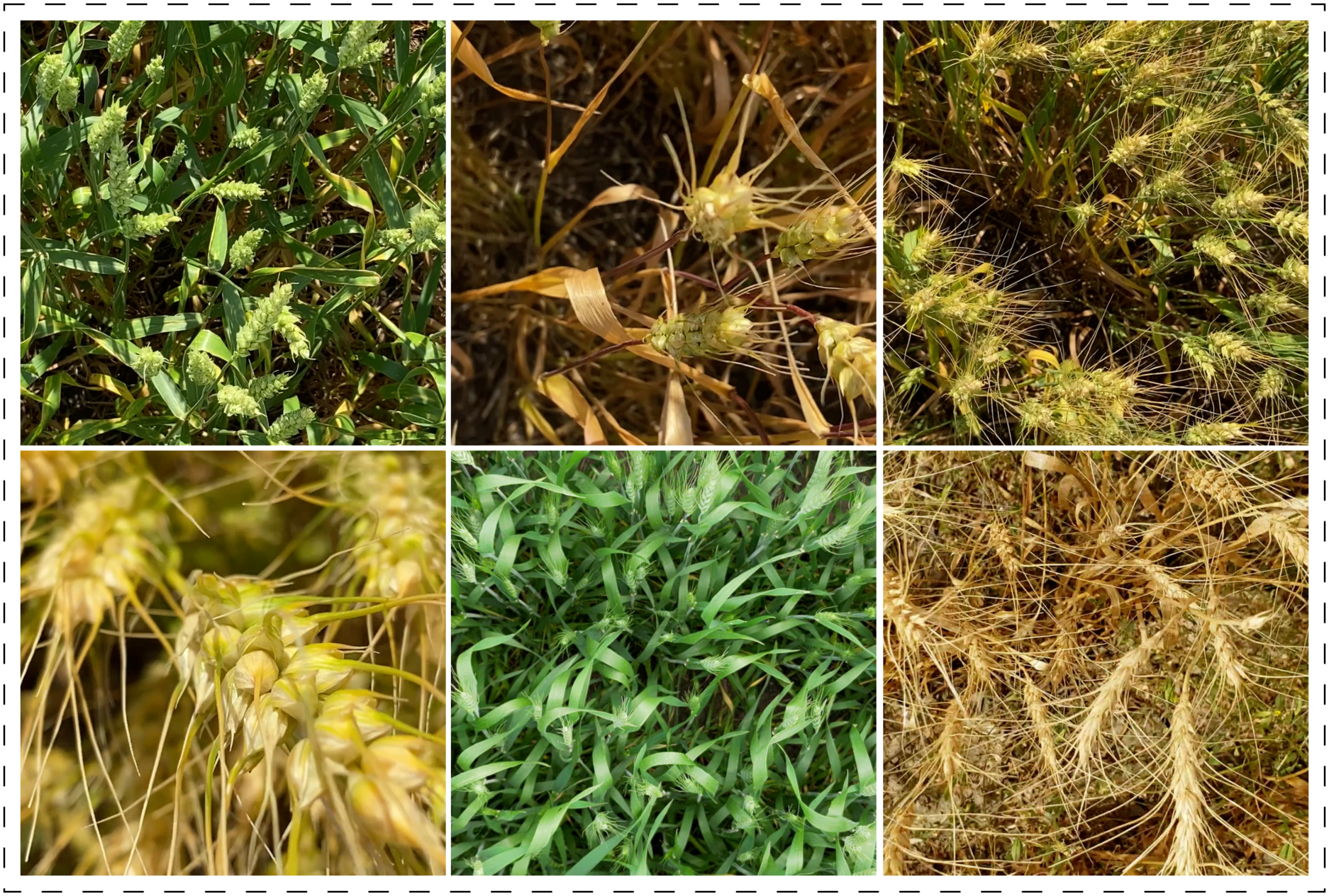
Figure 1: Depiction of diverse image frames capturing videos filmed at various altitudes via handheld cameras.

To maintain the coherence and consistency of visual elements, content, and object characteristics within each video and to reduce the computation complexity, we resized each frame from its original size of $2160\times 3840$ such that its height is scaled to $1024$ pixels while maintaining the aspect ratio, then center-crop it into the spatial size of $1024\times 1024$. Segmentation label for each frame was generated using the model detailed in [29]. Hereafter, we refer to this weakly labeled dataset as $\mathbb{W}=\Bigl{\{}\bigl{\{}(x_{t},y_{t})\mid 1\leq t\leq T_{i}\bigl{\}}\mid 1\leq i\leq n;V_{i}\in\mathbb{V}\Bigr{\}}$, where $T_{i}$ represent the number of video frames in video clip $V_{i}$.

A group-wise data split was conducted on $\mathbb{W}$ to partition it into training ($\mathbb{W}_{train}$), validation ($\mathbb{W}_{valid}$), and test ($\mathbb{W}_{test}$) sets. The group-wise data split was performed to ensure data points from one video clip are either in training, validation, or test set. Details of $\mathbb{W}_{train}$, $\mathbb{W}_{valid}$, and $\mathbb{W}_{test}$ are presented in Table 1.

Dataset	Notation	$\#$ of Videos	$\#$ of Frames	$\#$ of Annotated Frames
Training	$\mathbb{W}_{train}$	8	37,613	37,613
Validation	$\mathbb{W}_{valid}$	4	14,182	14,182
Testing	$\mathbb{W}_{test}$	5	34,777	34,777

Table 1: Summary of weakly labeled data.

2.1.2 Synthetic Dataset

In this research, we extended our prior work on image synthesization [28, 29] to simulate computationally annotated video clips, alleviating the challenge of manually annotating video clips, which is a laborious and resource-intensive process. In the following, we provide a detailed description of the methodology used for synthesizing these video clips.

We used a group of background videos ($\mathbb{B}$), which are fields without wheat crops exhibiting various vegetation types and environmental conditions. Figure 2 illustrates the process for extraction of the background video frames that will be used for synthesizing computationally annotated video clips. This is achieved by, first, randomly choosing video $B_{i}$ from the background videos $\mathbb{B}=\{B_{1},B_{2},\cdots B_{n}\}$. Then, $\tau$ consequent frames from $B_{i}$ are selected to form a set $B_{i,k}^{\prime}=\{b_{t}\mid k\leq t\leq k+\tau\textit{ and }1\leq k\leq T_{i}-\tau\}$. Next, a random region of size $1024\times 1024$ is chosen, and the crop defined by this region is extracted for all frames in $B_{i,k}^{\prime}$, resulting in a set of $\tau$ consecutive frames of size $1024\times 1024$, denoted as $C_{i,k}^{\prime}$.

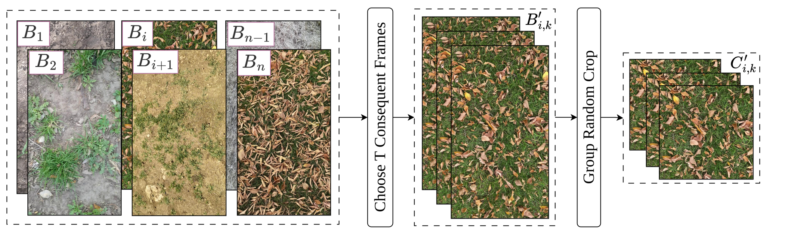
Figure 2: The procedure for extracting video frames from background videos $B_{i}\in\mathbb{B}$.

Additionally, we extracted wheat heads from a small number of manually annotated frames depicting both earlier growth stages in green shades and mature, harvestable stages in yellow coloration, resulting in a set of real wheat heads ($\mathbb{H}$) consisting of yellow (mature) and green (mid-season) wheat heads. Note that, for wheat head extraction, we chose the frames from three distinct videos that have no intersection with the $\mathbb{V}$ dataset. We also used extracted wheat heads in $\mathbb{H}$ as cookie-cutters to extract non-wheat head regions (fake wheat heads) from the original frames. This set is denoted as $\mathbb{\overline{H}}$. The presence of the fake wheat head prevents models from relying only on changes in intensity values and contrast for segmenting simulated video clips.

Figure 3 illustrates the process for synthesizing a manually annotated video clip. For set $C_{i,k}^{\prime}$ of $\tau$ consecutive background frames, a random number of fake and real wheat heads are chosen randomly from $\mathbb{\overline{H}}$ and $\mathbb{H}$, respectively. The fake wheat heads are overlaid on the first frame of $C_{i,k}^{\prime}$, and then real wheat heads are overlaid on the frame.

To simulate the movement and deformation of the crop, which naturally happens due to wind, we apply a sequence of spatial- and pixel-level transformations to each wheat head before overlying them on consecutive frames in $C_{i,k}^{\prime}$. These sequences of transformations are automatically generated for each wheat head to allow for consistency in movement while showing various degrees of deformations. More specifically, we define two types of movement for each wheat head object: object-level and frame-level movement. In object-level movement, we only updated the position and direction of each object individually. However, in the frame-level motion, all the objects’ positions will be adjusted with regard to the predefined motion behavior in the frame level.

This process results in synthesizing frames and their corresponding masks as we apply the special transformations and deformations to both the frame and mask, providing a consistent annotation for the resulting video clip. To create the mask corresponding to each synthesized video frame, a $1024\times 1024$ zero-value matrix is allocated for each of the $\tau$ frames in $C_{i,k}^{\prime}$. We keep track of the position of each real wheat head when overlaid on the background image and its movement and deformation to convert the corresponding region on the mask to 1. Note that the fake wheat heads are ignored.

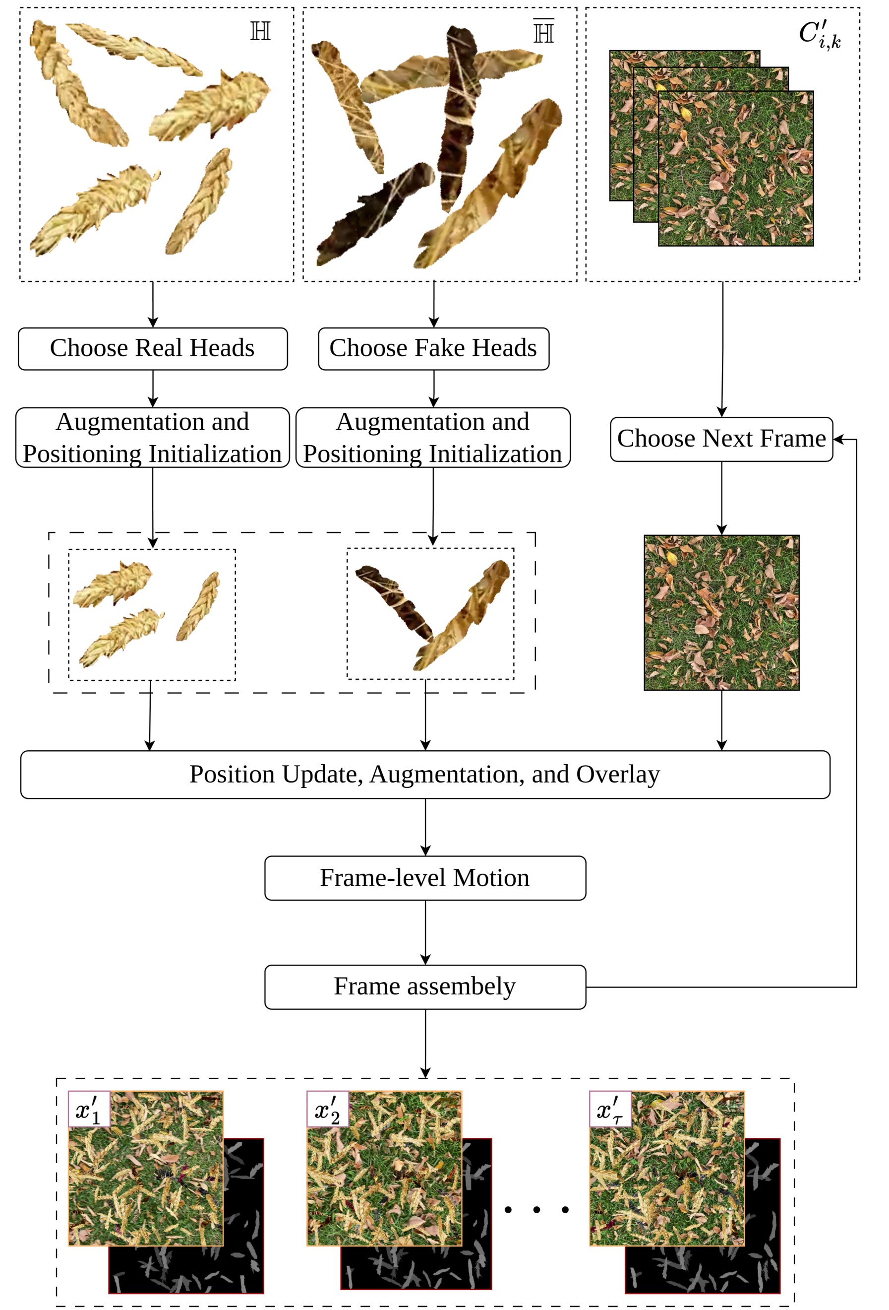
Figure 3: This diagram illustrates the process of synthesizing videos with dimensions of $1024\times 1024$ and a length of $T$. We generate a synthesized video $V^{\prime}$ by initializing a randomized selection of real and fake heads, each uniquely defined by augmentation and positioning parameters drawn from a pool of real and fake objects ($\mathbb{H}$ and $\mathbb{\overline{H}}$) overlaid on the first frame of $T$ randomly selected frames from $\{c_{t}\}_{t=i}^{i+T}$. Subsequent frames of $V^{\prime}$ are simulated based on the positions of wheat heads in the preceding frame, utilizing object-level and frame-level motion information. Objects that are removed are subsequently restored by incorporating additional real heads into the chosen object set by overlaying on the current frame before proceeding to the next frame. By applying the same object- and frame-level motions on the segmentation counters, the frame masks are also generated simultaneously.

Table 2: Summary of the synthetic videos and their frames distributions in the $\mathbb{S}_{train}$ dataset.

Dataset	Subset	$\#$ of Background Videos	$\#$ of Heads	$\#$ of Synthesized Videos	$\#$ of Frames
$\mathbb{S}_{train}$	Green Shaded	13	101	260	15600
	Yellow Shaded	15	251	600	36000

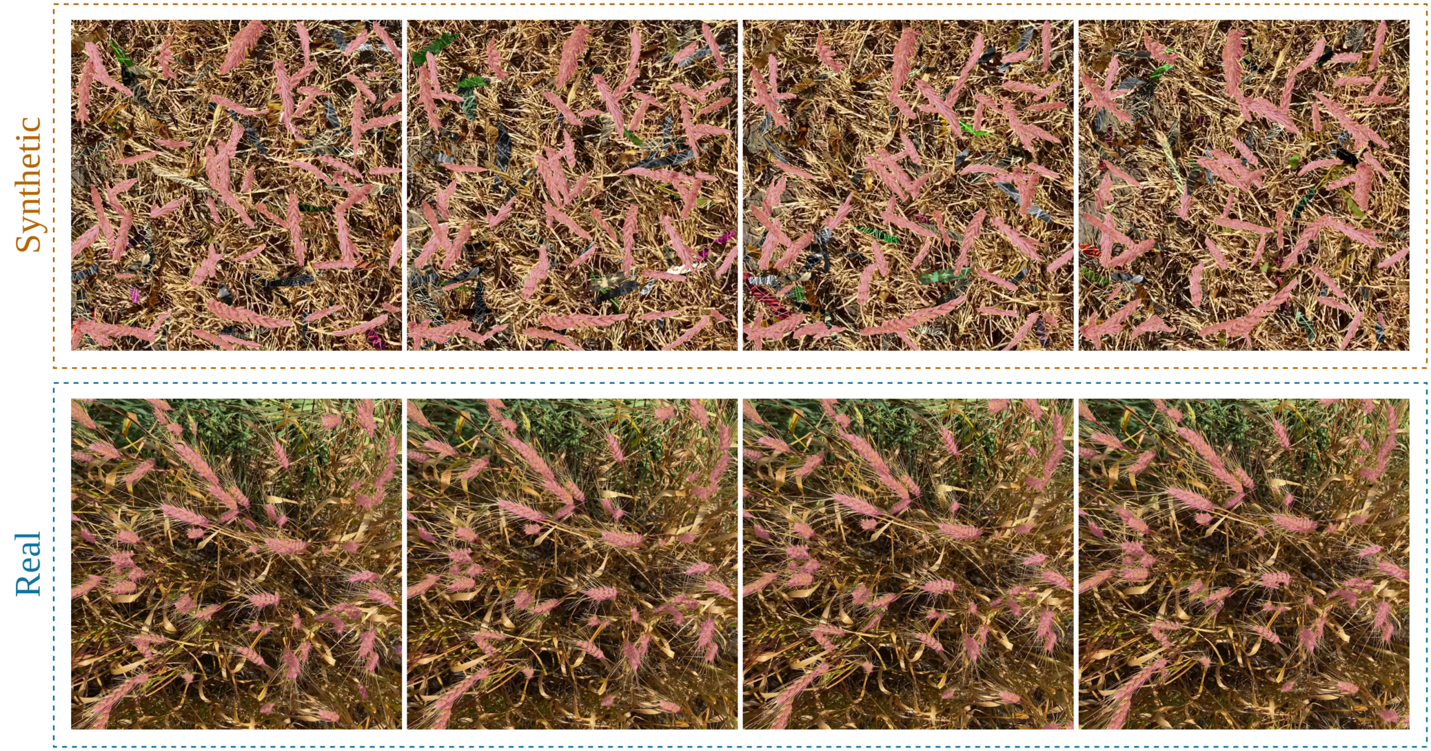
Figure 4: Visualization of synthetic versus real videos, left to right, with the time interval of $4$ seconds. The synthetic videos present a series of color-augmented fake wheat heads and masked real heads, isolated without wheat canopy and stems, overlaid on a sequence of uniform, flat background frames. These frames illustrate random head-level movements and synchronized frame-level dynamics. In contrast, the real videos depict actual wheat fields, capturing normal motion in dense-pattern wheat spikes attached to their stems and surrounded by wheat canopy including leaves and awns.

Figure 4 illustrates real and synthetic video frames, where their respective masks are annotated with pink color. This visualization highlights the systematic difference between real and simulated video clips, a phenomenon known as domain shift in the machine learning field, and often leads to a lack of generalizability, i.e., the model underperforms when applied to real unseen datasets. The rest of this section focuses on the data and methodology used for bridging this gap and alleviating domain shift.

2.2 Additional Datasets

We also used a validation set, $\Delta$, consisting of $300$ samples, which included five consecutive video frames where the first four frames are unannotated and the last one is annotated. The annotations were conducted in a semi-automated manner, where the predictions made by our prior model from [29] were manually refined as needed. Furthermore, we used a manually annotated set, $\Psi$, consisting of 100 samples for testing. Each sample in $\Psi$ includes a combination of five consecutive image frames, where the first four are unannotated, and the final one is manually annotated.

We also used an external test set, $\mathbb{D}$, of 48 samples, each containing five frames. The first four frames were unannotated, and the final frame was manually annotated.

These samples were extracted from three distinctly diverse drone-captured videos of wheat fields to evaluate the model performance on the pixel-accurate annotated images. Each drone video contributed $16$ samples to $\mathbb{D}$. The drone videos were captured using a DJI Mini 3 Pro Drone, from various altitudes. Figure 5 illustrates a few image frames from $\mathbb{D}$.

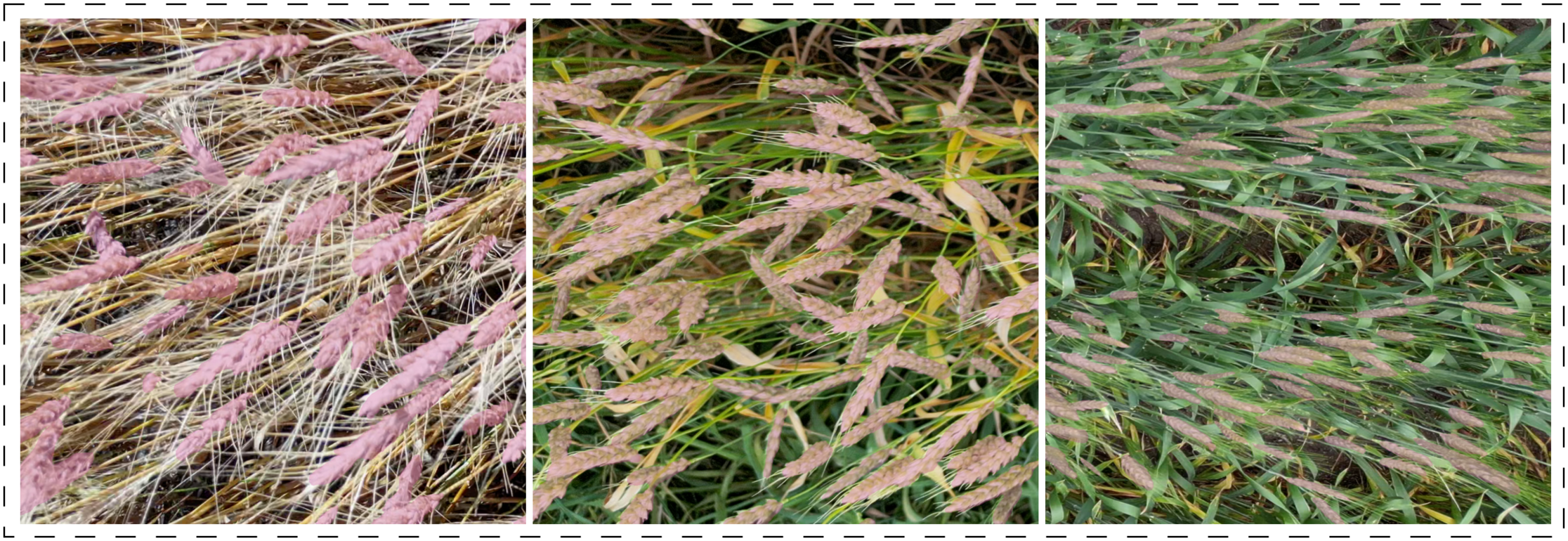
Figure 5: Depiction of human-annotated drone-captured video frames, overlaid by their masks in pink.

2.3 Model Architecture

We designed a UNet-style [39] architecture for DVOS by employing a multi-task training paradigm consisting of a segmentation task and an image reconstruction task. The architecture is designed to process a sequence of $\tau$ consecutive reference frames and predict the following frame and its mask. Hereafter, we refer to the $\tau$ reference frames as $\mathcal{R}$ and the query frame as $\mathcal{Q}$. Figure 6 illustrates the model architecture designed to perform both reconstruction and segmentation tasks simultaneously. This allows the model to utilize both spatial and temporal information for DVOS.

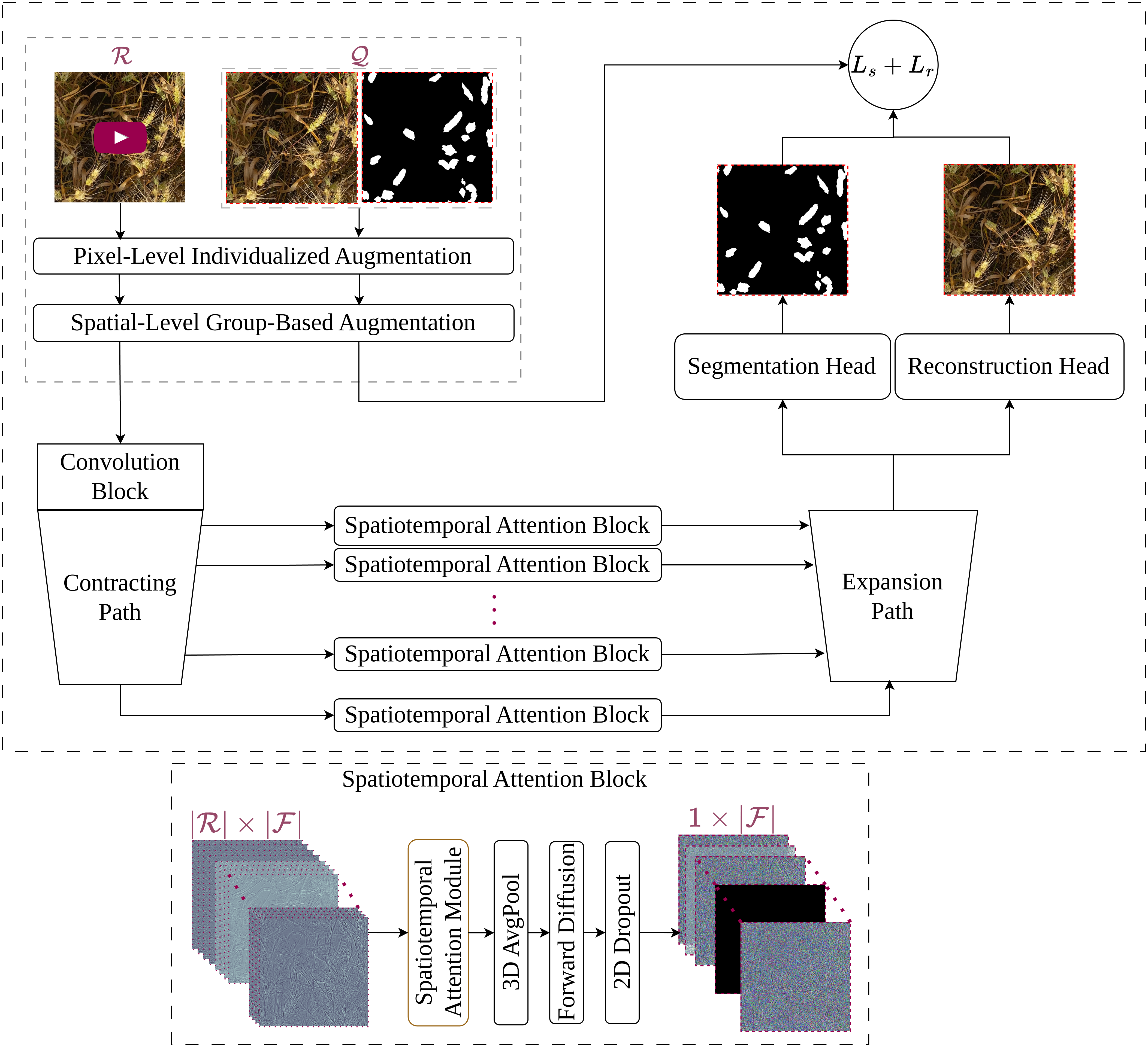
Figure 6: An overview of the proposed UNet-based [39] architecture for DVOS via prediction. The $|\mathcal{R}|$ feature map sets are concatenated and fed into the spatiotemporal attention module at each contracting level. Following this, channel reduction is achieved using a 3D pooling operation, noise is added through the forward diffusion process, and channel-wise dropout is applied before utilizing the unified feature maps in the expansion path. Feature maps derived from the latent space are subject to the same process, except for diffusion and dropout.

The proposed architecture processes the frames in $\mathcal{R}$ individually using a 2D convolutional neural network. The key components of the proposed architectures are an initial convolution block, a contraction path, skip attentions, skip diffusion, an expansion path, and decoder heads. In the following, we describe each component in detail.

The initial convolution block comprises a $3\times 3$ convolution layer, with stride 1 and padding 1, followed by two ResNet blocks (Figure 7). Each residual block consists of two consequent blocks. Each block comprises a Group Normalization [48] layer of size $8$, followed by Swish activation [34], and then a $3\times 3$ convolution with padding 1. Note that this initial convolution block does not change the spatial dimension of the input images.

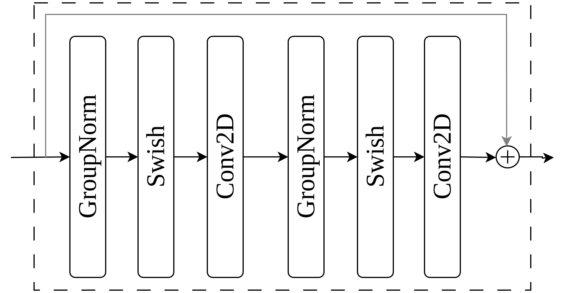
Figure 7: An overview of the residual building block, the base component of the proposed architecture.

The Contracting Path of the network is constructed of contractive blocks. Each contractive block is comprised of two residual blocks, followed by a $3$ convolution with the stride of $2$ and padding of $1$ for spatial downsampling. The output of each contractive block undergoes a Spatiotemporal Attention Block comprising a Spatiotemporal Attention Module, a channel reduction layer, followed by Skip Diffusion and Dropout layers.

The Spatiotemporal Attention Module, inspired by [17], aims at attending to the most informative signals from the $\tau=|\mathcal{R}|\times|\mathcal{F}|$ concatenated feature maps and generates one representative feature map. Figure 8 illustrates this module. It consists of two spatial and temporal attention streams combined to capture the spatial and temporal feature maps’ importance. The spatial attention stream consists of two blocks, each comprising a depth-wise separable convolution [13], followed by Group Normalization [19], and finally a Swish nonlinearity [34]. The temporal attention stream combines the $\tau$ feature maps using an adaptive average pooling across feature maps followed by two linear layers, wrapping a Swish non-linearity, and completed by a Sigmoid function.

The whole Spatiotemporal Attention Module is formulated in details by Formula 1, where Group Normalization is represented by $GN$, Depth-wise Seperable Convolution by $DSC$, Linear layers by $FC$, Adaptive Average Polling layer by $AvgPool$, $\mathcal{FM}$ is the input feature maps, $\mathcal{WFM}$ presents weighted feature maps, and the $dl$ notation indicates the dilation size.

$$S_{a}=Swish(GN(DSC^{dl=\cdot}(\cdot)))$$ (1)

$$T_{a}=FC(Swish(FC(AvgPool(\cdot))))$$

$$S=Sigmoid(S_{a}^{dl=2}(S_{a}^{dl=1}(\mathcal{FM}_{l})))$$

$$T=Sigmoid(T_{a}(\mathcal{S}))$$

$$\mathcal{WFM}_{l}=(T\odot S)\odot input$$

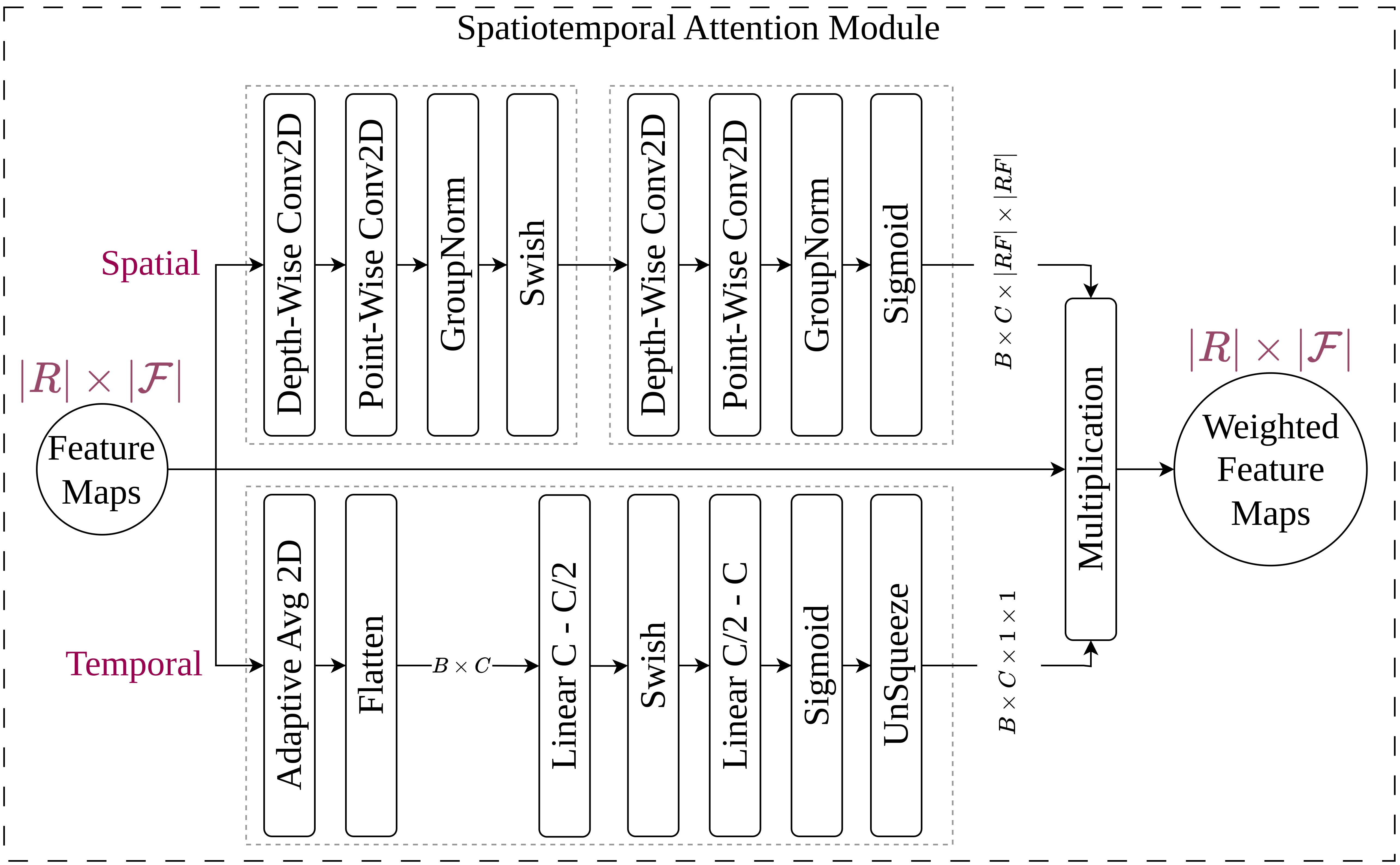
Figure 8: This figure illustrates the proposed spatiotemporal attention module, which incorporates two processing streams for input feature maps: (1) Spatial Attention Stream (Top) captures and weights informative spatial regions within individual reference frames. Group normalization is employed to highlight the spatial importance of feature maps corresponding to each input frame. Additionally, depth-wise separable convolutions are used for the efficient processing of large-scale feature maps; (2) the Temporal Attention Stream (Bottom) focuses on capturing temporal dynamics and dependencies. It weights each time step across feature maps extracted from all consecutive frames.

Given the concatenated feature maps $\mathcal{FM}_{l}$ of size $|\mathcal{R}|\times|\mathcal{F}|$, the Spatiotemporal Attention Module preserves the inputted feature map dimensions, $b\times c\times h\times w$. In this notation, $\mathcal{F}$ represents the features extracted for each input reference frame in $\mathcal{R}$ in downsampling level $l$. However, further processing of the attention output ($\mathcal{WFM}_{l}$) is required to achieve the desired output, addressing both dimensionality and feature quality concerns, before entering the Expansion path. Instead of employing feature dimension reduction using the $DSC$ layers, we opt to retain the entire input dimensionality and subsequently apply a 3D Average Pooling layer for this purpose. This process integrates spatiotemporal feature maps and generates feature maps of upsampling level channel size ($|\mathcal{F}|$). To prevent the model from excessively relying on skip connections as shortcuts, we introduce random noise to the feature maps using a diffusion-based noise scheduler, as detailed as follows. Additionally, we incorporate a random 2D Dropout layer with a specified probability to further increase randomization and mitigate the model maintaining the skip-connection shortcuts by randomly removing a subset of 2D feature maps.

Considering the unique design of the UNet architecture [39], skip connections enable the network to retain and reuse low- and high-level spatial information from earlier layers during decoding. This feature empowers UNet models for precise object localization by integrating high-resolution feature maps from the downscaling path with coarse semantic information from the upscaling path, leading to promising segmentation performance on clear input images. However, UNet models encounter challenges when reconstructing masked or noisy input images, or when predicting actual images or video frames, as they fail to operate rich semantic information obtained from the latent space [31]. This limitation arises from the model’s tendency to take shortcuts by transferring knowledge solely through high-resolution feature maps, thereby limiting its ability to effectively utilize the available mid-level information, on top of the other features, for reconstructing images properly.

Addressing this, we integrated a weighted version of the forward diffusion process into each of the skip connections aimed at balancing various-level feature contribution, thus enhancing the model’s reconstruction performance, improving the model’s representation learning capabilities, stabilizing the model’s training when exposed to synthetic data, as well as introducing an implicit domain adaptation mechanism by allowing the model to learn low-level and mid-level data features for reconstruction, rather than solely relying on low-level and high-level classification-related features for pixel-level classification. This approach diverges from generative diffusion models, which primarily focused on noise prediction [15, 52]. The integration follows the Markov process proposed in  [15].

$$x_{t}=\sqrt{\bar{\alpha_{t}}}x_{0}+\sqrt{1-\bar{\alpha}_{t}}\epsilon$$ (2)

where $q_{t}$ is sampled from the diffusion kernel, specified as $q\left(x_{t}|x_{0}\right)=\mathcal{N}\left(x_{t};\sqrt{\bar{\alpha}_{t}}x_{0},\left(1-\bar{\alpha}_{t}\right)\mathcal{I}\right)$. Here, $\epsilon\sim\mathcal{N}\left(0,\mathcal{I}\right)$, the scalar $\bar{\alpha}_{t}=\prod_{i=1}^{t}\left(1-\beta_{i}\right)$, and $\beta_{t}$ serves as the variance scheduler, formulated to ensure that $\bar{\alpha}_{T}\rightarrow 0$.

Commencing from the latent space, we initially refrain from applying noise to the feature maps. However, as we advance along the upsampling path of the network, noise augmentation intensifies at each level, corresponding to higher resolutions; hence, noise increases progressively. The noise level is regulated by selecting time steps $t$ from the beta probability density function. The beta distribution is a continuous probability distribution defined on the interval $[0,1]$. It is parameterized by two positive shape parameters, denoted by $\alpha$ and $\beta$.

$$f(x,\alpha,\beta)=\frac{1}{B\left(\alpha,\beta\right)}x^{\alpha-1}\left(1-x\right)^{\beta-1}$$ (3)

where $x\in[0,1]$, and $B\left(\alpha,\beta\right)$ is the beta function, which is a normalization constant that ensures the total area under the curve equals $1$. The beta function is also defined as follows:

$$B\left(\alpha,\beta\right)=\int_{0}^{1}t^{\alpha-1}(1-t)^{\beta-1}dt$$ (4)

Moreover, the mean and variance of the beta distribution are calculated as follows, which perfectly control the randomly generated time steps.

$$\mu=\frac{\alpha}{\alpha+\beta}$$ (5)

$$\sigma^{2}=\frac{\alpha\beta}{(\alpha+\beta)^{2}(\alpha+\beta+1)}$$ (6)

We established a scheduler to determine the values of $\alpha$ and $\beta$ for assigning distinct beta distribution functions to each level, thereby selecting diffusion time steps. This scheduling mechanism is governed by the following equations:

$$\alpha=\alpha_{0}+l$$ (7)

$$\beta=\beta_{0}-(\beta_{c}*l)$$ (8)

where $\alpha_{0}$, $\beta_{0}$ and $\beta_{c}$ represent initial and coefficient hyperparameters, and $l$ is the upsampling level index. which starts at the last skip connection, The index $l$ begins at the last skip connection and progresses towards the first skip connection, signifying the final upsampling step. Figure 9 depicts the shapes of beta distributions generated using our scheduler across varying values of $\alpha$ and $\beta$.

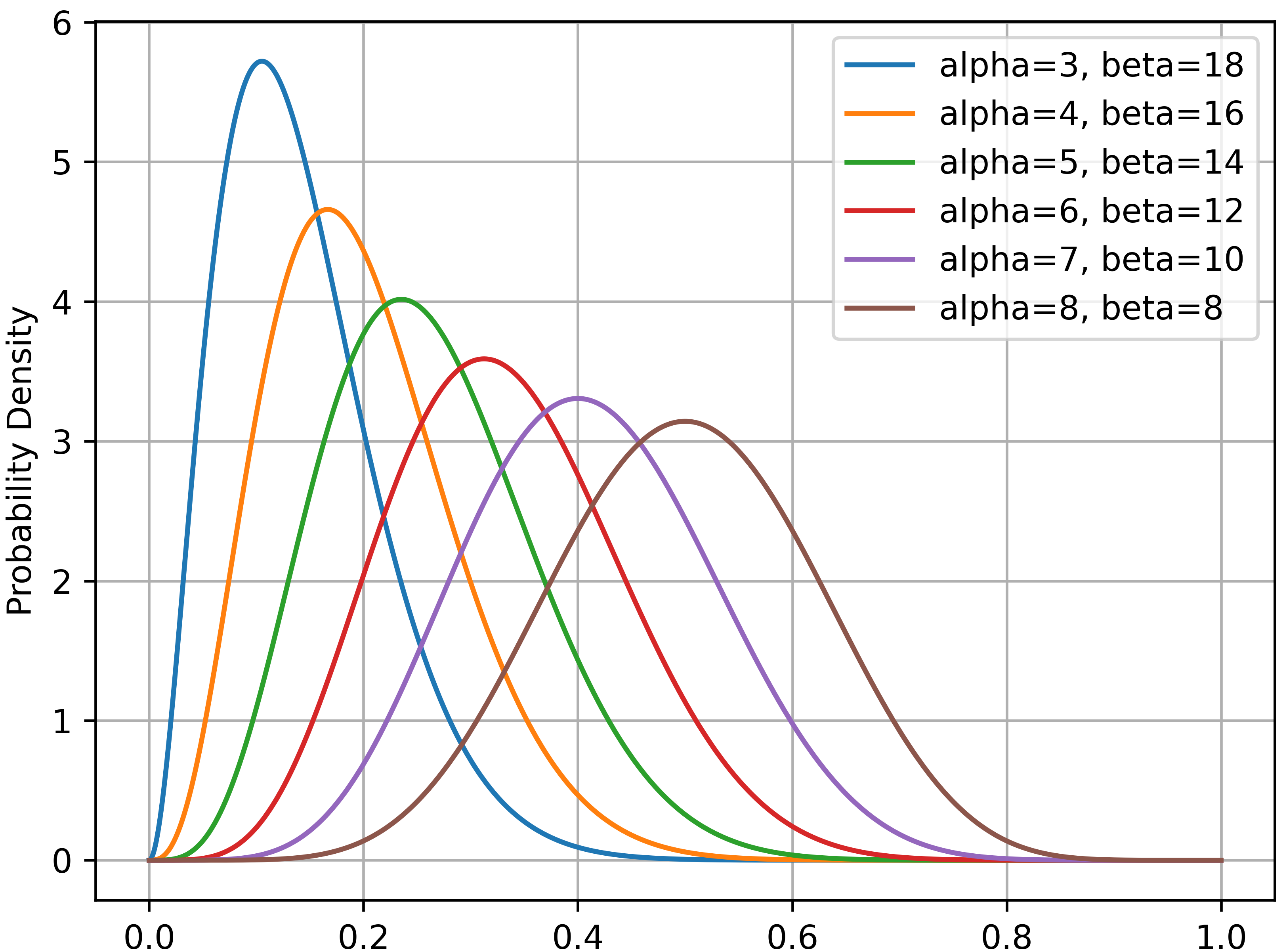
Figure 9: Visualization of Beta Distributions Generated by the Scheduler: This figure displays the shapes of beta distributions generated by our scheduler for various combinations of $\alpha$ and $\beta$ values. Each curve corresponds to a distinct beta distribution, illustrating the impact of parameter variation on the distribution’s shape. The curves are arranged from left to right for a model with six skip connections, progressing bottom-up from the latent space to the highest resolution of the upsampling path.

The decoder architecture within our model replicates the downsampling path, maintaining consistency in the number of residual locks at each level. However, it employs a nearest-neighbor operation with a scaling factor of two, followed by a single $3\times 3$ convolution operation, serving as the upsampling layer. Moreover, we leverage concatenation to integrate the skip connection and lower-resolution feature maps at each level. Functioning as a shared decoder for segmentation and reconstruction tasks, the UpScaling Path incorporates high-level semantic features within a localized context, while preserving spatial resolution from the latent space. This architecture adapts two decoding heads, each incorporating three residual blocks and one final $3\times 3$ convolution layer, ending in three-channel outputs for reconstruction and one-channel ones for segmentation.

2.4 Model Development and Training

We assessed the effectiveness and performance of our devised architecture on videos from a wider variety of domains. Yet, conventional UNet-style models demonstrate easily attainable promising performance in reconstructing clear inputs, with limitations concerning their utility in domain adaptation, image segmentation, and over-fitting mitigation. Consequently, we introduce a strategy involving diffusing input images in a patching style. This involves partitioning each whole reference frame in the mini-batch subjected to diffusion (with $P_{d}$ rate set to $0.5$) using the employed forward diffusion process [15], with random time steps limited to the range of $0$ to $1000$. Figure 10 displays a representative example of an input image subjected to the diffusion process.

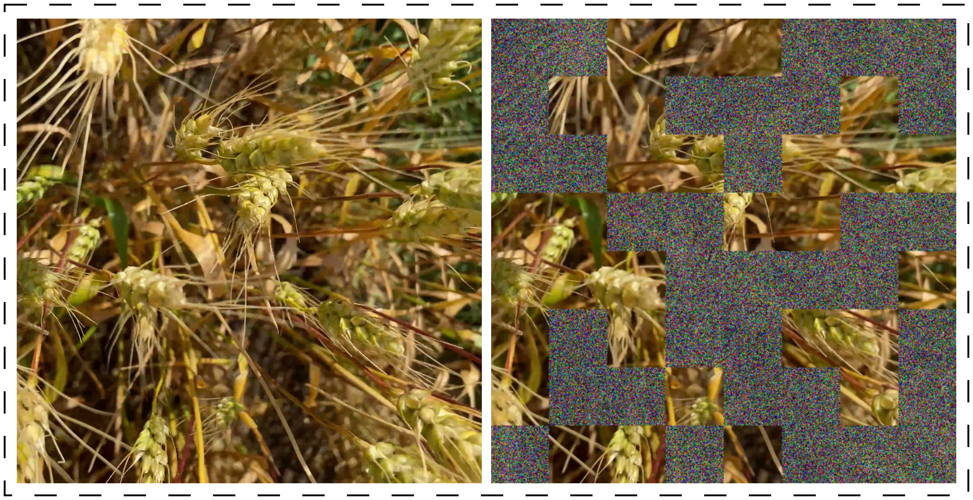
Figure 10: A depiction of an image frame alongside its diffused version, produced through the forward diffusion process.

In addition, we involved a pixel-level (color) argumentation transformation, only for reference frames, with light color-altering and blur transformations before applying the group-wise spatial transformations—including small-angle rotation, random cropping, and normalization—applied to reference frames and query frame/mask together.

We performed model training in two phases. We began the model development by training the $\mathbb{M}_{s}$ model from scratch on the $\mathbb{S}_{train}$ training datasets, with $\Delta$ serving as the validation set. Subsequently, in the second phase of training, we fine-tune the $\mathbb{M}_{s}$ model on the weakly-labeled $\mathbb{W}_{train}$ and $\mathbb{W}_{valid}$ datasets, yielding our final model denoted as $\mathbb{M}_{w}$.

In this study, we utilized two commonly used segmentation metrics, Dice and Intersection over Union (IoU) scores for segmentation evaluation. Additionally, we utilized Mean Squared Error (MSE or L2) and Structural Similarity Index (SSIM) losses together for reconstruction ($L_{r}$ in Figure 6), and Binary Cross Entropy (BCE) and Dice losses ($L_{s}$ in Figure 6) jointly for segmentation. Due to the substantial dataset sizes, we trained each model for $15$ epochs and selected the model with the highest validation Dice score as the best-performing model for further evaluation. We exploited the AdamW optimizer [23] with a learning rate of $1e-4$, weight decay of $1e-5$ in the first training phase, and no weight decay in the second phase for $\mathbb{M}_{w}$.

We employed randomly sized squared-shape crops ranging between $400$ to $750$ from the original $1024\times 1024$ image frames, resizing them to the training size of $256$ for training purposes. However, during evaluation, we replaced the random cropping operations with a single center crop operation of size $512$ to ensure consistency across all epochs and model development phases for validation and test sets.

3 Results

Table 3 demonstrates the performance of developed models across our test sets. Model $\mathbb{M}_{s}$ was exclusively trained on the computationally annotated synthetic dataset, whereas the model $\mathbb{M}_{w}$ was trained on real but weakly-labeled wheat field videos. Despite being trained solely with the synthetic dataset, $\mathbb{M}_{s}$ demonstrates reasonably high performance across all three datasets. Furthermore, model $\mathbb{M}_{s}$, which was trained on precisely annotated data for image/mask prediction, exhibits superior performance on the manually-labeled datasets ($\Psi$ and $\mathbb{D}$) compared to the pseudo-labeled dataset ($\mathbb{W}_{test}$). This potentially reflects the true pixel-level segmentation efficacy of the model, as indicated by the pixel-accurate annotation of these datasets.

Table 3: Quantitative results of the developed DVOS models ($\mathbb{M}_{s}$, $\mathbb{M}_{w}$) on diverse test sets.

Model	Trained On	Test Set	IoU	Dice
$\mathbb{M}_{s}$	None	$\Psi$	0.389	0.543
		$\mathbb{W}_{test}$	0.220	0.337
		$\mathbb{D}$	0.417	0.578
$\mathbb{M}_{w}$	$\mathbb{M}_{s}$	$\Psi$	0.546	0.699
		$\mathbb{W}_{test}$	0.609	0.736
		$\mathbb{D}$	0.700	0.821

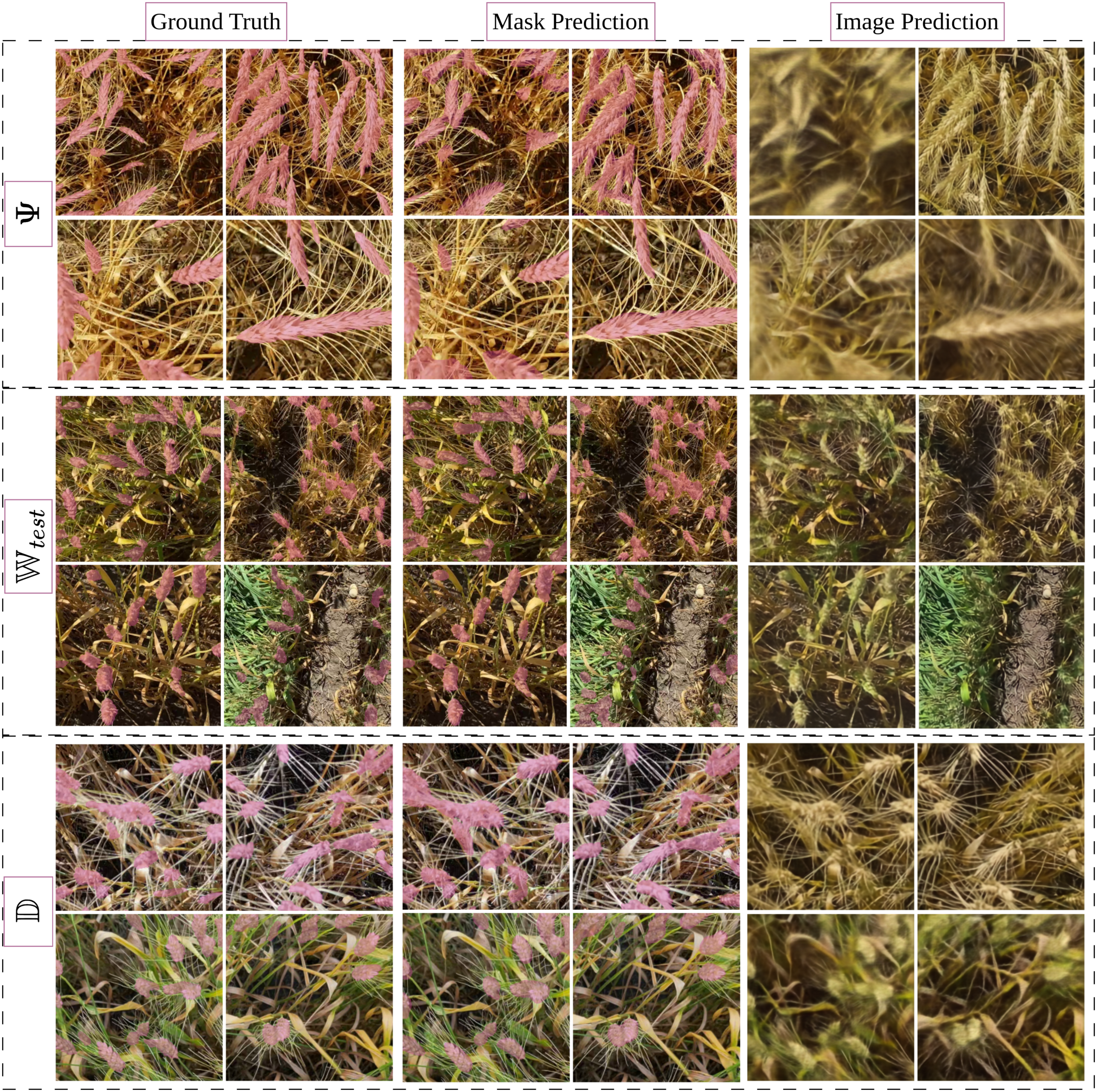
Figure 11: Performance visualization of the $\mathbb{M}_{w}$ model across different test sets. The first two columns depict masks overlaid on the corresponding images. Each block forms $4$ different samples, which are visualized in the same grid cell across Ground Truth, Mask Prediction, and Image Prediction columns.

Additionally, these findings highlight the relatively close performance of model $\mathbb{M}_{s}$ across both human-annotated test sets, underscoring the practical utility of synthetic data in video model development. Notably, our synthesis process utilized only a limited selection of wheat heads from a few samples spanning two domains. Despite this constraint, the model demonstrates relatively similar performance across the phenotypically diverse dataset $\mathbb{W}_{test}$, which consists of videos captured from varying altitudes, as well as different weather conditions and light levels, affirming its high degree of generalizability.

Our fine-tuned model, $\mathbb{M}_{w}$, exhibits notably improved performance when trained on the large-scale and diverse weakly-labeled dataset, $\mathbb{W}_{train}$, achieving a substantial performance gain of over $15.6\%$ on $\Psi$ dataset, despite lacking training samples from this domain, and nearly $39.9\%$ on $\mathbb{W}_{test}$. Furthermore, the model’s accuracy on the manually labeled dataset underscores its precision in pixel-accurate segmentation of wheat head objects. This model also demonstrates significantly enhanced performance when evaluated on $\mathbb{D}$, achieving a Dice score of $0.821$. This represents an improvement of over $26\%$ compared to model $\mathbb{M}_{s}$.

Figure 11, visually, illustrates the prediction performance of model $\mathbb{M}_{w}$ on randomly selected samples from the test sets. A grid format is used to arrange four randomly selected samples in each block. The first and third rows show the prediction performance, the second and third columns, of the model while the first column represents the manually annotated labels. However, the first column of the second row shows the weak (model-generated) masks overlaid on the images. Note that, we solely used the frame prediction power of the model for model training; however, the model performs well in predicting the query frame in the existence of hierarchically added skip-level noise.

Table 4: Quantitative results of the developed models ($\mathbb{M}_{s}$, $\mathbb{M}_{w}$), on individual videos from $\mathbb{W}_{test}$.

Model	Trained On	Test Set	IoU	Dice
$\mathbb{M}_{s}$	None	Video 1	0.164	0.247
		Video 2	0.252	0.387
		Video 3	0.234	0.360
		Video 4	0.156	0.260
		Video 5	0.148	0.226
$\mathbb{M}_{w}$	$\mathbb{M}_{s}$	Video 1	0.390	0.548
		Video 2	0.636	0.763
		Video 3	0.798	0.887
		Video 4	0.785	0.878
		Video 5	0.780	0.867

We also conducted individual evaluations of the model $\mathbb{M}_{w}$ performance on each video $\mathbb{V}\in\mathbb{W}_{test}$, each capturing a diverse exhibition of wheat plants, collectively, from diverse phenotypes, often from slightly variant altitudes. While the model demonstrates consistent performance across most videos, Video 1 proves more challenging to segment in comparison to the others (see Figure 12). This difficulty is evident in the performance of both models ($\mathbb{M}_{s}$, $\mathbb{M}_{w}$). Particularly, the presence of low-quality video leads to impaired weakly-labeled ground truth, thereby diminishing the quantitative scores of our models. Despite this, visual inspection reveals the proper model segmentation of Video 1, capturing the wheat heads, even those of the lowest quality. However, the model segments tighter regions covering each wheat head compared to the ground truth, which includes a broader area—wrapping each wheat head—and including many false positives.

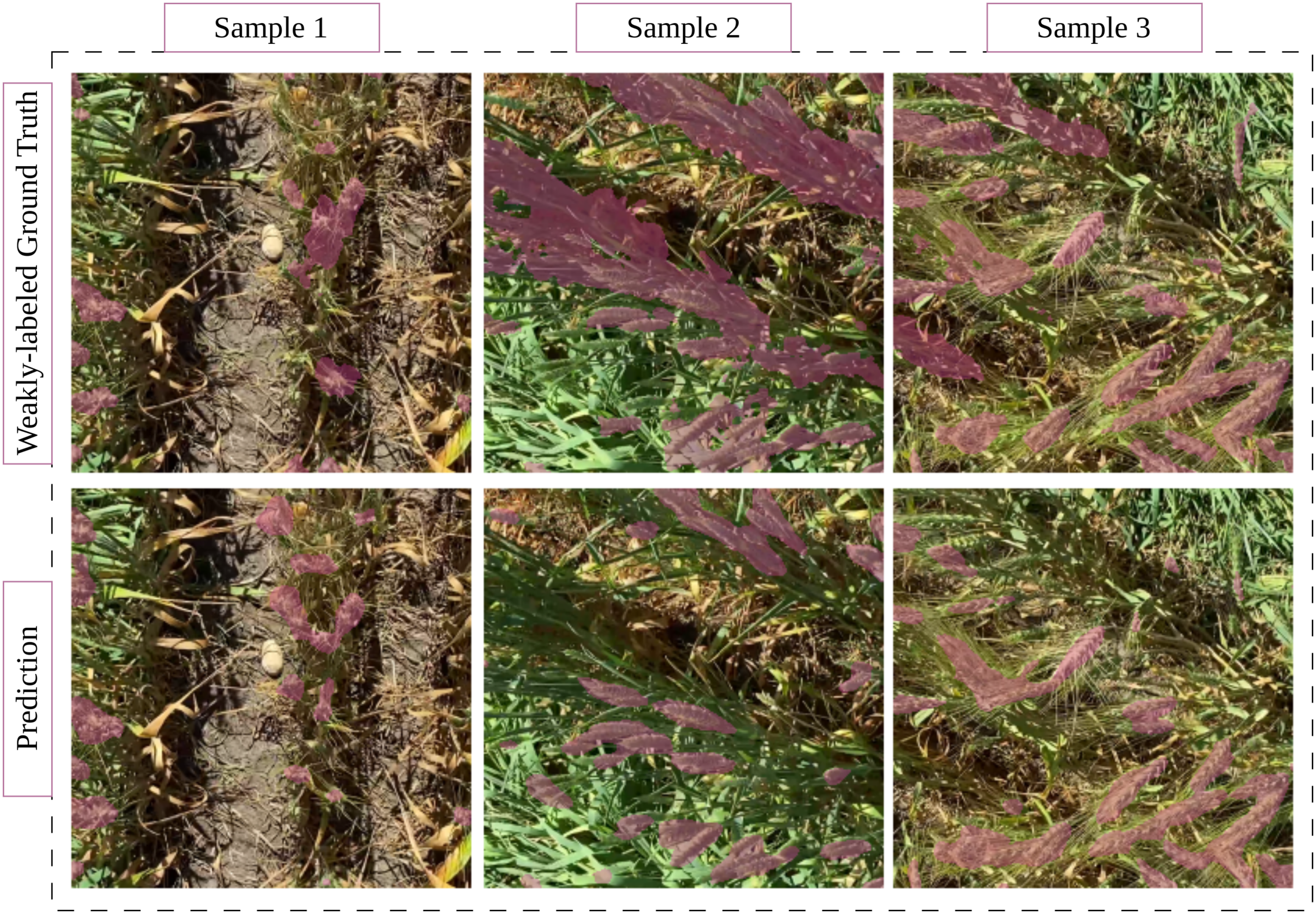
Figure 12: The prediction performance of model $\mathbb{M}_{w}$ on the $\textit{Video 1}\in\mathbb{W}_{test}$ (second row) compared to their weakly-labeled ground truth (first row). The samples in each column show the mismatches between the ground truth and predictions, causing a significant reduction in model performance on this video compared to the other videos in this set.

4 Discussion

In this study, we proposed a semi-self-supervised learning methodology to develop a novel model architecture designed for segmenting videos with dense patterns. Our approach is semi-supervised as it involves the initial training of the model using computationally annotated synthesized videos that were exclusively generated from wheat heads extracted from seven annotated frames originating from two domains. Additionally, our methodology is self-supervised, as we utilized model-generated annotations (weak labels) for further model development. We also incorporated self-supervised image prediction alongside mask prediction during model training. By utilizing synthesized and weakly labeled videos for model development, we circumvented the labor-intensive process of manual segmentation for high-frame-rate videos capturing dense and small objects.

We introduced a novel architecture for Dense Video Object Segmentation (DVOS) tasks. This architecture integrates a hierarchical diffusion process as its core and employs a spatiotemporal mechanism for object segmentation through multi-task image/mask prediction. Specifically, we devised a new UNet-style [39, 31] architecture with reduced parameters achieved through shared encoders and decoders. This architecture features two distinct heads for frame and mask prediction, enhancing efficiency in utilizing shared decoder feature maps and robustness during model training.

In VOS, most studies [8, 25, 38, 26, 5, 6] incorporate the segmentation masks of reference frames as auxiliary inputs of their network. To be more specific, they employ the manual annotation of the videos’ initial frame, coupled with either human- or model-generated segmentation maps for subsequent reference frames, and then utilize them within the encoder, decoder, or both components of the network, with the ultimate objective of generating the segmentation mask corresponding to $\mathcal{Q}$. In this work, however, we fed solely the reference image frames to the model and employed only the query mask as the ground truth. We exclusively leverage weak masks, derived from an image-based segmentation model [29], as opposed to relying on manual or VOS-model generated segmentation labels.

We designed our methodology and the architecture concerning a few main challenges:

• Transferring the unprocessed high-level features, preferred for segmentation, through the skip connections [31], UNet-style models [39] ignore integrating rich latent feature maps, appropriate for reconstruction. The effect is less pronounced in images containing a single large-size object of interest, compared to domains with densely packed, repetitive small objects. Also, videos, captured in uncontrolled environments using either handheld or unmanned aerial vehicles such as drones, are often influenced by environmental factors such as wind and sunshine and present a higher level of noise compared to individually captured images. Therefore, we integrated a diffusion-based data preprocessing strategy as well as a hierarchical diffusion process as the core of our proposed architecture. This way we tried to regulate the data flow within the network, completed by the adoption of a standard forward diffusion process to simulate noisy inputs. By incorporating these methodologies, we enhanced the model’s robustness to input noise, consequently improving the quality of reconstructed images (Third column of Figure 11) and leading to more effective model training and, finally, segmentation outcomes.

• We transformed the VOS task into a multi-task learning framework for frame and mask prediction. Through reconstruction losses, our objective was to integrate an explicit domain adaptation process into the model development. This process pushed the model to acquire middle-level feature maps necessary for reconstructing the input image frame, thus adapting to various visual patterns, enhanced by input data augmentation, and improving the model’s generalizability. Furthermore, by training the model on relatively simple synthetic data and employing reconstruction losses, we mitigated the risk of overfitting, thereby enhancing the regularization effect in the model training process.

• We chose data synthesis with automatic annotation over the tedious process of manual data annotation. Simulating the motion and optical flow characteristics of real-world captured videos, we devised a video synthesis strategy to generate a diverse and large-scale dataset of computationally annotated videos. Here, we extended the data synthesis proposed in [29] by adding object-level and frame-level motions to the current frame to generate the subsequent frames. We generated a consistent number of short video clips from various regions of each of the background videos to construct a well-balanced large-scale dataset. This dataset holds videos with diverse backgrounds, thereby boosting the generalizability of the developed model, demonstrated by mode $\mathbb{M}_{s}$ in table 3.

• Additionally, we proceeded to fine-tune the model using real-world examples paired with weak masks. This refinement process resulted in a notable enhancement in model performance, with improvements ranging between $15\%$ to $20\%$ across various test sets. The multi-task training strategy, coupled with our specifically designed architecture, enabled the model to learn the precise boundaries of small and densely packed objects of interest. By reconstructing future image frames and their corresponding segmentations based on provided previous reference frames, the model achieved greater performance on our manually labeled dataset ($\mathbb{D}_{\Upsilon}$).

Although model $\mathbb{M}_{w}$ was trained on synthetic data and fine-tuned on the weakly-labeled data (sampled in the first row of Figure 12), the second row of this figure demonstrates its accuracy in properly segmenting wheat heads. This indicates the robustness of the model’s training process, as it effectively disregards misleading segmentation signals in the weakly labeled data and focuses on multi-level and semantic features in our defined multi-task segmentation/reconstruction training paradigm. In addition, the performance of the models in this video is significantly lower than the other videos, which encompass clips of higher quality. This further highlights the critical importance of video quality in developing, evaluating, and deploying models in real-world environments.

In this study, our model development process relied exclusively on synthesized data accompanied by computationally generated annotations. We used only five manually annotated video frames highlighted in yellow from one distribution, supplemented by two additional green-shaded frames from another distribution. We declare that augmenting the dataset with more wheat head objects extracted from frames of diverse wheat domains with higher resolutions would further enhance the model’s performance. Additionally, by extracting wheat heads from individually captured images rather than from noisy, out-of-focus, or blurry video frames, we could obtain clearer wheat head objects, resulting in higher-quality synthetic data. We adopted a straightforward approach to overlaying wheat heads, prioritizing minimal movement relationships between heads. Strengthen the relationship and more synchronized wheat head movements could potentially improve the authenticity of the wheat field videos, and yield a better performance.

In addition, in the second phase of model development, we use authentic but weakly labeled videos for model fine-tuning. In other words, the model was not trained using pixel-level accurate human-annotated data. Furthermore, the weakly labeled dataset included primarily long video clips, each representing only a limited number of phenotypically distinguished domains. Given these constraints, we recommend expanding the scope of our proposed architecture by incorporating a broader collection of shorter video clips capturing a more diverse range of data domains.

In this work, we showed the utility of synthetic video clips with pixel-accurate annotation, alone, for model development ($\mathbb{M}_{s}$). Developing models from scratch using only weakly labeled video frames, even on such an extensive scale, poses a notable challenge in determining and extracting informative patterns or features from the input data, providing misleading signals. Therefore, using only a few samples from two domains for data synthesis, we experimented with the capability of the developed model to obtain reasonably high performance even when trained on such computationally annotated and uniform synthetic data. We believe that increasing the quantity and diversity of human-annotated images, used for foreground real and fake object extraction ($\mathbb{H}$, $\overline{\mathbb{H}}$), enhances the diversity of synthetic data, thereby, results in significant improvement in model performance.

Considering the flexibility, scalability, and learning adaptability of our proposed architecture and the well-designed data synthesis pipeline, we suggest the exploration of this approach across various research domains beyond wheat crop DVOS. For instance, applications in medical imaging and other data modalities within precision agriculture hold promise for leveraging the capabilities of our architecture. Furthermore, our architecture presents an adaptable solution applicable to any domain necessitating precise semantic segmentation coupled with domain adaptation requirements, such as autonomous driving scenarios.

5 Conclusion

In conclusion, our study presented a novel semi-self-supervised strategy for developing Dense Video Segmentation (DVS) models. Our methodology addressed the challenges associated with annotating dense, small, and partially occluded objects within video frames, a notoriously tedious process. More specifically, we leveraged a multi-task frame/mask prediction architecture, computationally annotated synthesized videos, and real-looking videos with weak labels for model training. We also demonstrated its promising utility in precision agriculture, particularly for wheat spike Video Object Segmentation. Notably, despite relying on a limited number of human-annotated video frames, our models achieved high performances across diverse test sets. Importantly, we discussed that the proposed methodology can be extended beyond precision agriculture. Its applicability contains domains requiring video-centric tasks with multiple objects and dense patterns, such as autonomous driving and medical imaging.

References

- Alkhudaydi et al. [2019] Tahani Alkhudaydi, Daniel Reynolds, Simon Griffiths, Ji Zhou, and Beatriz De La Iglesia. An exploration of deep-learning based phenotypic analysis to detect spike regions in field conditions for UK bread wheat. Plant Phenomics, 2019, 2019.
- Ariza-Sentís et al. [2023] Mar Ariza-Sentís, Hilmy Baja, Sergio Vélez, and João Valente. Object detection and tracking on uav rgb videos for early extraction of grape phenotypic traits. Computers and Electronics in Agriculture, 211:108051, 2023.
- Bhagat et al. [2021] Sandesh Bhagat, Manesh Kokare, Vineet Haswani, Praful Hambarde, and Ravi Kamble. WheatNet-Lite: A novel light weight network for wheat head detection. In Proceedings of the IEEE/CVF International Conference on Computer Vision, pages 1332–1341, 2021.
- Campos et al. [2016] Yerania Campos, Humberto Sossa, and Gonzalo Pajares. Spatio-temporal analysis for obstacle detection in agricultural videos. Applied Soft Computing, 45:86–97, 2016.
- Cheng and Schwing [2022] Ho Kei Cheng and Alexander G Schwing. Xmem: Long-term video object segmentation with an atkinson-shiffrin memory model. In European Conference on Computer Vision, pages 640–658. Springer, 2022.
- Cheng et al. [2021] Ho Kei Cheng, Yu-Wing Tai, and Chi-Keung Tang. Rethinking space-time networks with improved memory coverage for efficient video object segmentation. Advances in Neural Information Processing Systems, 34:11781–11794, 2021.
- Ciga et al. [2022] Ozan Ciga, Tony Xu, and Anne Louise Martel. Self supervised contrastive learning for digital histopathology. Machine Learning with Applications, 7:100198, 2022.
- Dai et al. [2016] Jifeng Dai, Kaiming He, and Jian Sun. Instance-aware semantic segmentation via multi-task network cascades. In Proceedings of the IEEE Conference on computer Vision and Pattern Recognition, pages 3150–3158, 2016.
- Das and Bais [2021] Mohana Das and Abdul Bais. DeepVeg: Deep learning model for segmentation of weed, canola, and canola flea beetle damage. IEEE Access, 9:119367–119380, 2021.
- David et al. [2021] Etienne David, Mario Serouart, Daniel Smith, Simon Madec, Kaaviya Velumani, Shouyang Liu, Xu Wang, Francisco Pinto, Shahameh Shafiee, Izzat SA Tahir, et al. Global wheat head detection 2021: An improved dataset for benchmarking wheat head detection methods. Plant Phenomics, 2021, 2021.
- Gibbs et al. [2019] Jonathon A. Gibbs, Alexandra Jacquelyn Burgess, Michael P. Pound, Tony P. Pridmore, and Erik Harry Murchie. Recovering wind-induced plant motion in dense field environments via deep learning and multiple object tracking1[cc-by]. Plant Physiology, 181:28 – 42, 2019.
- Goodfellow et al. [2014] Ian Goodfellow, Jean Pouget-Abadie, Mehdi Mirza, Bing Xu, David Warde-Farley, Sherjil Ozair, Aaron Courville, and Yoshua Bengio. Generative adversarial nets. Advances in Neural Information Processing Systems, 27, 2014.
- Guo et al. [2019] Yunhui Guo, Yandong Li, Liqiang Wang, and Tajana Rosing. Depthwise convolution is all you need for learning multiple visual domains. In Proceedings of the AAAI Conference on Artificial Intelligence, pages 8368–8375, 2019.
- Han and Li [2022] Feixiang Han and Jie Li. Wheat heads detection via YOLOv5 with weighted coordinate attention. In 2022 7th International Conference on Cloud Computing and Big Data Analytics (ICCCBDA), pages 300–306. IEEE, 2022.
- Ho et al. [2020] Jonathan Ho, Ajay Jain, and Pieter Abbeel. Denoising diffusion probabilistic models. Advances in Neural Information Processing Systems, 33:6840–6851, 2020.
- Ho et al. [2022] Jonathan Ho, William Chan, Chitwan Saharia, Jay Whang, Ruiqi Gao, Alexey Gritsenko, Diederik P Kingma, Ben Poole, Mohammad Norouzi, David J Fleet, et al. Imagen video: High definition video generation with diffusion models. arXiv preprint arXiv:2210.02303, 2022.
- Hu et al. [2018] Jie Hu, Li Shen, and Gang Sun. Squeeze-and-excitation networks. In Proceedings of the IEEE Conference on Computer Vision and Pattern Recognition, pages 7132–7141, 2018.
- Hu et al. [2021] Li Hu, Peng Zhang, Bang Zhang, Pan Pan, Yinghui Xu, and Rong Jin. Learning position and target consistency for memory-based video object segmentation. In Proceedings of the IEEE/CVF Conference on Computer Vision and Pattern Recognition, pages 4144–4154, 2021.
- Ioffe and Szegedy [2015] Sergey Ioffe and Christian Szegedy. Batch normalization: Accelerating deep network training by reducing internal covariate shift. In International Conference on Machine Learning, pages 448–456. pmlr, 2015.
- Koprinska and Carrato [2001] Irena Koprinska and Sergio Carrato. Temporal video segmentation: A survey. Signal processing: Image communication, 16(5):477–500, 2001.
- Lipton and Lipton [2021] Lenny Lipton and Lenny Lipton. The zoëtrope and the praxinoscope. The Cinema in Flux: The Evolution of Motion Picture Technology from the Magic Lantern to the Digital Era, pages 55–60, 2021.
- Liu et al. [2021] Ze Liu, Yutong Lin, Yue Cao, Han Hu, Yixuan Wei, Zheng Zhang, Stephen Lin, and Baining Guo. Swin transformer: Hierarchical vision transformer using shifted windows. In Proceedings of the IEEE/CVF International Conference on Computer Vision, pages 10012–10022, 2021.
- Loshchilov and Hutter [2017] Ilya Loshchilov and Frank Hutter. Decoupled weight decay regularization. arXiv preprint arXiv:1711.05101, 2017.
- Ma et al. [2020] Juncheng Ma, Yunxia Li, Hongjie Liu, Keming Du, Feixiang Zheng, Yongfeng Wu, and Lingxian Zhang. Improving segmentation accuracy for ears of winter wheat at flowering stage by semantic segmentation. Computers and Electronics in Agriculture, 176:105662, 2020.
- Maninis et al. [2018] K-K Maninis, Sergi Caelles, Yuhua Chen, Jordi Pont-Tuset, Laura Leal-Taixé, Daniel Cremers, and Luc Van Gool. Video object segmentation without temporal information. IEEE Transactions on Pattern Analysis and Machine Intelligence, 41(6):1515–1530, 2018.
- Meinhardt and Leal-Taixé [2020] Tim Meinhardt and Laura Leal-Taixé. Make one-shot video object segmentation efficient again. Advances in Neural Information Processing Systems, 33:10607–10619, 2020.
- Myers et al. [2024] Jaden Myers, Keyhan Najafian, Farhad Maleki, and Katie Ovens. Modified cyclegan for the synthesization of samples for wheat head segmentation. arXiv preprint arXiv:2402.15135, 2024.
- Najafian et al. [2021] Keyhan Najafian, Ali Ghanbari, Ian Stavness, Lingling Jin, Gholam Hassan Shirdel, and Farhad Maleki. A semi-self-supervised learning approach for wheat head detection using extremely small number of labeled samples. 2021 IEEE/CVF International Conference on Computer Vision Workshops (ICCVW), pages 1342–1351, 2021.
- Najafian et al. [2022] Keyhan Najafian, Alireza Ghanbari, Mahdi Sabet Kish, Mark G. Eramian, Gholam Hassan Shirdel, Ian Stavness, Lingling Jin, and Farhad Maleki. Semi-self-supervised learning for semantic segmentation in images with dense patterns. Plant Phenomics, 5, 2022.
- Nguyen-Thai et al. [2021] Binh Nguyen-Thai, Vuong Le, Catherine Morgan, Nadia Badawi, T. Tran, and Svetha Venkatesh. A spatio-temporal attention-based model for infant movement assessment from videos. IEEE Journal of Biomedical and Health Informatics, 25:3911–3920, 2021.
- Oktay et al. [2018] Ozan Oktay, Jo Schlemper, Loic Le Folgoc, Matthew Lee, Mattias Heinrich, Kazunari Misawa, Kensaku Mori, Steven McDonagh, Nils Y Hammerla, Bernhard Kainz, et al. Attention u-net: Learning where to look for the pancreas. arXiv preprint arXiv:1804.03999, 2018.
- Perazzi et al. [2016] Federico Perazzi, Jordi Pont-Tuset, Brian McWilliams, Luc Van Gool, Markus Gross, and Alexander Sorkine-Hornung. A benchmark dataset and evaluation methodology for video object segmentation. In Proceedings of the IEEE Conference on Computer Vision and Pattern Recognition, pages 724–732, 2016.
- Perazzi et al. [2017] Federico Perazzi, Anna Khoreva, Rodrigo Benenson, Bernt Schiele, and Alexander Sorkine-Hornung. Learning video object segmentation from static images. In Proceedings of the IEEE Conference on Computer Vision and Pattern Recognition, pages 2663–2672, 2017.
- Ramachandran et al. [2017] Prajit Ramachandran, Barret Zoph, and Quoc V. Le. Swish: a self-gated activation function. arXiv: Neural and Evolutionary Computing, 2017.
- Rawat et al. [2022] Shivangana Rawat, Akshay L Chandra, Sai Vikas Desai, Vineeth N Balasubramanian, Seishi Ninomiya, and Wei Guo. How useful is image-based active learning for plant organ segmentation? Plant Phenomics, 2022, 2022.
- Real et al. [2017] Esteban Real, Jonathon Shlens, Stefano Mazzocchi, Xin Pan, and Vincent Vanhoucke. Youtube-boundingboxes: A large high-precision human-annotated data set for object detection in video. In proceedings of the IEEE Conference on Computer Vision and Pattern Recognition, pages 5296–5305, 2017.
- Redmon and Farhadi [2018] Joseph Redmon and Ali Farhadi. Yolov3: An incremental improvement. ArXiv, abs/1804.02767, 2018.
- Robinson et al. [2020] Andreas Robinson, Felix Jaremo Lawin, Martin Danelljan, Fahad Shahbaz Khan, and Michael Felsberg. Learning fast and robust target models for video object segmentation. In Proceedings of the IEEE/CVF Conference on Computer Vision and Pattern Recognition, pages 7406–7415, 2020.
- Ronneberger et al. [2015] Olaf Ronneberger, Philipp Fischer, and Thomas Brox. U-net: Convolutional networks for biomedical image segmentation. In Medical Image Computing and Computer-Assisted Intervention–MICCAI 2015: 18th International Conference, Munich, Germany, October 5-9, 2015, Proceedings, Part III 18, pages 234–241. Springer, 2015.
- Sabzi et al. [2019] Sajad Sabzi, Yousef Abbaspour-Gilandeh, Jose Luis Hernandez-Hernandez, Farzad Azadshahraki, and Rouhollah Karimzadeh. The use of the combination of texture, color and intensity transformation features for segmentation in the outdoors with emphasis on video processing. Agriculture, 9(5):104, 2019.
- Sadeghi-Tehran et al. [2019] Pouria Sadeghi-Tehran, Nicolas Virlet, Eva M Ampe, Piet Reyns, and Malcolm J Hawkesford. DeepCount: in-field automatic quantification of wheat spikes using simple linear iterative clustering and deep convolutional neural networks. Frontiers in Plant Science, 10:1176, 2019.
- Tan et al. [2020] Changwei Tan, Pengpeng Zhang, Yongjiang Zhang, Xinxing Zhou, Zhixiang Wang, Ying Du, Wei Mao, Wenxi Li, Dunliang Wang, and Wenshan Guo. Rapid recognition of field-grown wheat spikes based on a superpixel segmentation algorithm using digital images. Frontiers in Plant Science, 11:259, 2020.
- Tan et al. [2023] Cheng Tan, Zhangyang Gao, Lirong Wu, Yongjie Xu, Jun Xia, Siyuan Li, and Stan Z Li. Temporal attention unit: Towards efficient spatiotemporal predictive learning. In Proceedings of the IEEE/CVF Conference on Computer Vision and Pattern Recognition, pages 18770–18782, 2023.
- Ubbens et al. [2020] Jordan R Ubbens, Tewodros W Ayalew, Steve Shirtliffe, Anique Josuttes, Curtis Pozniak, and Ian Stavness. Autocount: Unsupervised segmentation and counting of organs in field images. In European Conference on Computer Vision, pages 391–399. Springer, 2020.
- Ullah et al. [2021] Hafiz Sami Ullah, Muhammad Hamza Asad, and Abdul Bais. End to end segmentation of canola field images using dilated U-Net. IEEE Access, 9:59741–59753, 2021.
- Vondrick et al. [2016] Carl Vondrick, Hamed Pirsiavash, and Antonio Torralba. Generating videos with scene dynamics. Advances in Neural Information Processing Systems, 29, 2016.
- Wang et al. [2024] Chien-Yao Wang, I-Hau Yeh, and Hong-Yuan Mark Liao. Yolov9: Learning what you want to learn using programmable gradient information. arXiv preprint arXiv:2402.13616, 2024.
- Wu and He [2018] Yuxin Wu and Kaiming He. Group normalization. In Proceedings of the European Conference on Computer Vision (ECCV), pages 3–19, 2018.
- Yamaguchi et al. [2021] Shin’ya Yamaguchi, Sekitoshi Kanai, Tetsuya Shioda, and Shoichiro Takeda. Image enhanced rotation prediction for self-supervised learning. In 2021 IEEE International Conference on Image Processing (ICIP), pages 489–493. IEEE, 2021.
- Yang et al. [2021] Charig Yang, Hala Lamdouar, Erika Lu, Andrew Zisserman, and Weidi Xie. Self-supervised video object segmentation by motion grouping. In Proceedings of the IEEE/CVF International Conference on Computer Vision, pages 7177–7188, 2021.
- Yang et al. [2018] Linjie Yang, Yanran Wang, Xuehan Xiong, Jianchao Yang, and Aggelos K Katsaggelos. Efficient video object segmentation via network modulation. In Proceedings of the IEEE Conference on Computer Vision and Pattern Recognition, pages 6499–6507, 2018.
- Yang et al. [2023] Ling Yang, Zhilong Zhang, Yang Song, Shenda Hong, Runsheng Xu, Yue Zhao, Wentao Zhang, Bin Cui, and Ming-Hsuan Yang. Diffusion models: A comprehensive survey of methods and applications. ACM Computing Surveys, 56(4):1–39, 2023.
- Yang et al. [2022] Xiangli Yang, Zixing Song, Irwin King, and Zenglin Xu. A survey on deep semi-supervised learning. IEEE Transactions on Knowledge and Data Engineering, 35(9):8934–8954, 2022.
- Zbontar et al. [2021] Jure Zbontar, Li Jing, Ishan Misra, Yann LeCun, and Stéphane Deny. Barlow twins: Self-supervised learning via redundancy reduction. In International Conference on Machine Learning, pages 12310–12320. PMLR, 2021.
- Zhang et al. [2023] Yurong Zhang, Liulei Li, Wenguan Wang, Rong Xie, Li Song, and Wenjun Zhang. Boosting video object segmentation via space-time correspondence learning. In Proceedings of the IEEE/CVF Conference on Computer Vision and Pattern Recognition, pages 2246–2256, 2023.