GR-Athena++: magnetohydrodynamical evolution with dynamical space-time

Abstract

We present a self-contained overview of GR-Athena++, a general-relativistic magnetohydrodynamics (GRMHD) code, that incorporates treatment of dynamical space-time, based on the recent work of Daszuta+ Daszuta:2021ecf and Cook+ Cook:2023bag . General aspects of the Athena++ framework we build upon, such as oct-tree based, adaptive mesh refinement (AMR) and constrained transport, together with our modifications, incorporating the $\mathrm{Z}4$c formulation of numerical relativity, judiciously coupled, enables GRMHD with dynamical space-times. Initial verification testing of GR-Athena++ is performed through benchmark problems that involve isolated and binary neutron star space-times. This leads to stable and convergent results. Gravitational collapse of a rapidly rotating star through black hole formation is shown to be correctly handled. In the case of non-rotating stars, magnetic field instabilities are demonstrated to be correctly captured with total relative violation of the divergence-free constraint remaining near machine precision. The use of AMR is show-cased through investigation of the Kelvin-Helmholtz instability which is resolved at the collisional interface in a merger of magnetised binary neutron stars. The underlying task-based computational model enables GR-Athena++ to achieve strong scaling efficiencies above $80\%$ in excess of $10^{5}$ CPU cores and excellent weak scaling up to $\sim 5\times 10^{5}$ CPU cores in a realistic production setup. GR-Athena++ thus provides a viable path towards robust simulation of GRMHD flows in strong and dynamical gravity with exascale high performance computational infrastructure.

0.1 Introduction

Embedding the techniques of numerical relativity (NR) within robust, highly-performant simulation infrastructure provides an indispensable tool for understanding the phenomenology of astrophysical inspiral and merger events. This is especially pertinent due to the arrival of multimessenger astronomy observations. Indeed recent, near-simultaneous detections of the gravitational wave signal GW170817, and associated electromagnetic counterpart GRB 170817A, alongside a kilonova, resulting from the merger of a Binary Neutron Star (BNS) system, have been made TheLIGOScientific:2017qsa ; Goldstein:2017mmi ; Savchenko:2017ffs . These two events provide insight on the astrophysical origins of short Gamma Ray bursts (SGRB) as ensuing from BNS progenitors Monitor:2017mdv .

The end products of BNS mergers have long been viewed as candidates for the launching of relativistic jets giving rise to SGRBs Blinnikov:1984a ; Paczynski:1986px ; Goodman:1986a ; Eichler:1989ve ; Narayan:1992iy however the precise mechanism remains an open question. The presence of large magnetic fields in a post-merger remnant may play a role in jet formation Piran:2004ba ; Kumar:2014upa ; Ciolfi:2018tal . Such fields may arise as the result of magnetohydrodynamic (MHD) instabilities during the late inspiral such as the Kelvin-Helmholtz instability (KHI) Rasio:1999a ; Price:2006fi ; Kiuchi:2015sga , magnetic winding, and the Magneto-Rotational Instability (MRI) Balbus:1991a . The configuration of magnetic fields for a BNS system during the early inspiral is an open question. Already in the case of an isolated neutron star an initially poloidal field can give rise to instability Tayler:1957a ; Tayler:1973a ; Wright:1973a ; Markey:1973a ; Markey:1974a ; Flowers:1977a , and long-term simulations involving isolated stars suggest that higher resolution is required to understand reasonable initial configurations for the magnetic fields Kiuchi:2008ss ; Ciolfi:2011xa ; Ciolfi:2013dta ; Lasky:2011un ; Pili:2014npa ; Pili:2017yxd ; Sur:2021awe , with thermal effects also playing a key role in the evolution of the field Pons:2019zyc .

The distribution and nature of matter outflow from a BNS merger may also be influenced by the presence of magnetic fields Siegel:2014ita ; Kiuchi:2014hja ; Siegel:2017nub ; Mosta:2020hlh ; Curtis:2021guz ; Combi:2022nhg ; deHaas:2022ytm ; Kiuchi:2022nin ; Combi:2023yav . These outflows determine the nature of the long lived electromagnetic signal following merger, such as AT2017gfo which accompanied GW170817 GBM:2017lvd ; Coulter:2017wya ; Soares-santos:2017lru ; Arcavi:2017xiz , known as the kilonova Li:1998bw ; Kulkarni:2005jw ; Metzger:2010sy , as well as the r-process nucleosynthesis responsible for heavy element production occurring in ejecta Pian:2017gtc ; Kasen:2017sxr . It is clear that understanding the evolution of a BNS system from its late inspiral, through merger, to the post-merger is a formidable endeavour. A broad range of physical processes must be modeled consistently that include general relativity (GR), MHD, weak nuclear processes leading to neutrino emission and reabsorption, and the finite temperature behaviour of dense nuclear matter.

For the solution of the Einstein field equations, two commonly utilized classes of free evolution formulations of NR are: those based on moving puncture gauge conditions Brandt:1997tf ; Campanelli:2005dd ; Baker:2005vv , such as BSSN Shibata:1995we ; Baumgarte:1998te , Z4c Bernuzzi:2009ex ; Ruiz:2010qj ; Weyhausen:2011cg ; Hilditch:2012fp , and CCZ4 formulations Alic:2011gg ; Alic:2013xsa ; and the Generalised Harmonic Gauge approach Pretorius:2005gq . These may be coupled to MHD so as to provide a system of GRMHD evolution equations. In this context the ideal MHD limit of a non-resistive and non-viscous fluid is typically assumed. The aforementioned are written as a system of balance laws, which is key for shock capture and mass conservation Font:2007zz . In order to preserve the magnetic field divergence-free condition a variety of approaches have been considered: Constrained Transport (CT) Evans:1988a ; Ryu:1998ar ; Londrillo:2003qi ; Flux-CT Toth:2000 ; vector potential formulation Etienne:2011re ; and divergence cleaning  Dedner:2002a . Extensive effort has been invested into constructing codes for GRMHD simulation involving such techniques, a (non-exhaustive) list of examples include Baiotti:2004wn ; Duez:2005sf ; Shibata:2005gp ; Anderson:2006ay ; Giacomazzo:2007ti ; Duez:2008rb ; Liebling:2010bn ; Foucart:2010eq ; Thierfelder:2011yi ; East:2011aa ; Loffler:2011ay ; Moesta:2013dna ; Radice:2013xpa ; Etienne:2015cea ; Kidder:2016hev ; Palenzuela:2018sly ; Vigano:2018lrv ; Cipolletta:2019geh ; Cheong:2020kpv ; Shankar:2022ful . Aside from the complexity of the underlying physics modeled, a further important concern for NR based investigations is efficient resolution of solution features that develop over widely disparate scales that scale when simulations utilize high performance computing (HPC) infrastructure.

To this end we overview and demonstrate the recently developed GRMHD capabilities of our code GR-Athena++ Daszuta:2021ecf ; Cook:2023bag . We build upon a public version of Athena++ Stone:2020 which is an astrophysical (radiation), GRMHD, c++ code for stationary space-times that features a task-based computational model built to exploit hybrid parallelism through dual use of message passing interface MPI and threading via OpenMP. Our efforts embed the $\mathrm{Z}4$c formulation suitably coupled to GRMHD thereby removing the stationarity restriction. This allows GR-Athena++ to evolve magnetised BNS. To this end we leverage the extant Athena++ infrastructure and methods such as CT. We inherit block-based, adaptive mesh refinement (AMR) capabilities which exploit (binary, quad, oct)-tree structure with synchronisation restricted to layers at block boundaries. This can be contrasted against other codes utilizing AMR with fully-overlapping, nested grids that rely on the Berger-Oliger Berger:1984zza ; Berger:1989a time subcycling algorithm.

On account of this GR-Athena++ can efficiently resolve features developing during the BNS merger, such as small scale structures in the magnetic field instabilities, without requiring large scale refinement of coarser features. Performance scaling is demonstrated to $\mathcal{O}(10^{5})$ CPU cores, showing efficient utilization of exascale HPC architecture.

0.2 Code overview

GR-Athena++ builds upon Athena++ thus in order to specify nomenclature, provide a self-contained description, and explain our extensions, we first briefly recount some details of the framework (see also White:2015omx ; felker2018fourthorderaccuratefinite ; Stone:2020 ).

In Athena++, overall details about the domain $\Omega$ over which a problem is formulated are abstracted from the salient physics and contained within a class called the Mesh. Within the Mesh an overall representation of the domain as a logical $n$-rectangle is stored, together with details of coordinatization type (Cartesian or more generally curvilinear), number of points along each dimension for the coarsest sampling $N_{M}=(N_{M_{1}},\,\cdots,\,N_{M_{d}})$, and physical boundary conditions on $\partial\Omega$. Next, we would like to decompose the domain into smaller blocks, described by so-called MeshBlock objects. In order to partition the domain we first fix a choice $N_{B}=(N_{B_{1}},\,\cdots,\,N_{B_{d}})$ where each element of $N_{B}$ must divide each element of $N_{M}$ component-wise. Then $\Omega$ is domain-decomposed through rectilinear sub-division into a family of $n$-rectangles satisfying $\Omega=\sqcup_{i\in Z}\Omega_{i}$, where $Z$ is the set of MeshBlock indices, corresponding to the ordering described in §0.2.1. Nearest-neighbor elements are constrained to only differ by a single sub-division at most. The MeshBlock class stores properties of an element $\Omega_{i}$ of the sub-division. In particular the number of points in the sampling of $\Omega_{i}$ is controlled through the choice of $N_{B}$. For purposes of communication of data between nearest neighbor MeshBlock objects the sampling over $\Omega_{i}$ is extended by a thin layer of so-called “ghost nodes” in each direction. Furthermore the local values (with respect to the chosen, extended sampling on $\Omega_{i}$) of any discretized, dependent field variables of interest are stored within the MeshBlock.

In both uniform grid $(\forall i\in Z)$ $\mathrm{vol}(\Omega_{i})=C$ and refined meshes $(\exists i,\,j\in Z)$ $\mathrm{vol}(\Omega_{i})\neq\mathrm{vol}(\Omega_{j})$ it is crucial to arrange inter-MeshBlock communication efficiently – to this end the relationships between differing MeshBlock objects are arranged in a tree data structure, to which we now turn.

0.2.1 Tree structure of the Mesh

For the sake of exposition here and convenience in later sections we now particularize to a Cartesian coordinatization though we emphasize that the general picture (and our implementation) of the discussions here and in §0.2.2 carry over to the curvilinear context with only minor modification.

(GR-)Athena++ stores the logical relationship between the MeshBlock objects (i.e. $\Omega_{i}$) involved in description of a domain $\Omega$ within a tree data structure. A binary-tree, quad-tree or oct-tree is utilized when $d:=\dim(\Omega)=1,\,2,\,3$ respectively. The relevant tree is then constructed by first selecting the minimum $N$ such that $2^{N}$ exceeds the largest number of $\Omega_{i}$ along any dimension. The root of the tree is assigned a logical level of zero and the tree terminates at level $N$ with every MeshBlock assigned to an appropriate leaf, though some leaves and nodes of the tree may remain empty. Data locality is enhanced, as references to MeshBlock objects are stored such that a post-order, depth-first traversal of the tree follows Morton order (also termed Z-order) morton1966computer . This order can be used to encode multi-dimensional coordinates into a linear index parametrizing a Z-shaped, space-filling curve where small changes in the parameter imply spatial coordinates that are close in a suitable sense burstedde2019numberfaceconnectedcomponents .

As an example we consider a three-dimensional Mesh described by $(N_{x},\,N_{y},\,N_{z})=(2,\,5,\,3)$ MeshBlock objects in each direction at fixed physical level in Fig.1.

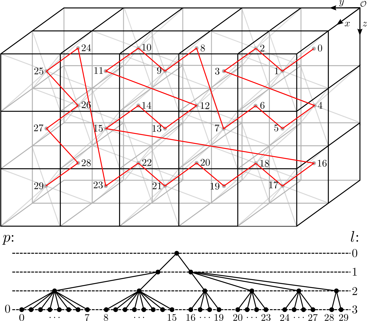
Figure 1: Example of Mesh partitioned uniformly by MeshBlock objects indexed via Z-order and traced in red through constituent geometric centroids. The logical relationship between $\Omega_{i}$ is stored in an oct-tree. Empty leaves are suppressed though each populated node above logical level three has eight children. Notice that physical level $p$ and logical level $l$ are distinct. (Figure adapted from Daszuta:2021ecf ).

Mesh refinement

In order to resolve solution features over widely varying spatial (temporal) scales (GR-)Athena++ implements block-based adaptive mesh refinement (AMR) stout1997adaptiveblockshigh . This naturally fits into the domain-decomposition structure previously described as each physical position on a computational domain is covered by one and only one level. Salient field data need only be synchronized at block (MeshBlock) boundaries. The logical arrangement into a (binary,quad,oct)-tree structure has the added benefit of improving computational efficiency through preservation of data locality in memory. Similarly the underlying task-based parallelism (see §0.3.6) as the computational model greatly facilitates the overlap of communication and computation.

Consider now a Mesh with refinement. The number of physical refinement levels added to a uniform level, domain-decomposed $\Omega$ is controlled by the parameter $N_{L}$. By convention $N_{L}$ starts at zero. Subject to satisfaction of problem-dependent, user-prescribed, refinement criteria, there may exist physical levels at $0,\,\cdots,\,N_{L}$. When a given MeshBlock is refined (coarsened) $2^{d}$ MeshBlock objects are constructed (destroyed). This is constrained to satisfy a $2:1$ refinement ratio where nearest-neighbor MeshBlock objects can differ by at most one physical level. Function data at a fixed physical level is transferred one level finer through use of a prolongation operator $\mathcal{P}$; dually, function data may be coarsened by one physical level through restriction $\mathcal{R}$. The details of the $\mathcal{P}$ and $\mathcal{R}$ operators depend on the underlying field treated, together with the selection of discretization.

A concrete example of a potential overall structure is provided in Fig.2 where we consider a non-periodic $\Omega$ described by $N_{x}=N_{y}=N_{z}=2$ MeshBlock objects with $N_{L}=3$ selected with refinement introduced at the corner $x_{\max}$, $z_{\max}$. If periodicity conditions are imposed on $\partial\Omega$ then additional refinement may be required for boundary intersecting MeshBlock objects so as to maintain the aforementioned inter-MeshBlock $2:1$ refinement ratio.

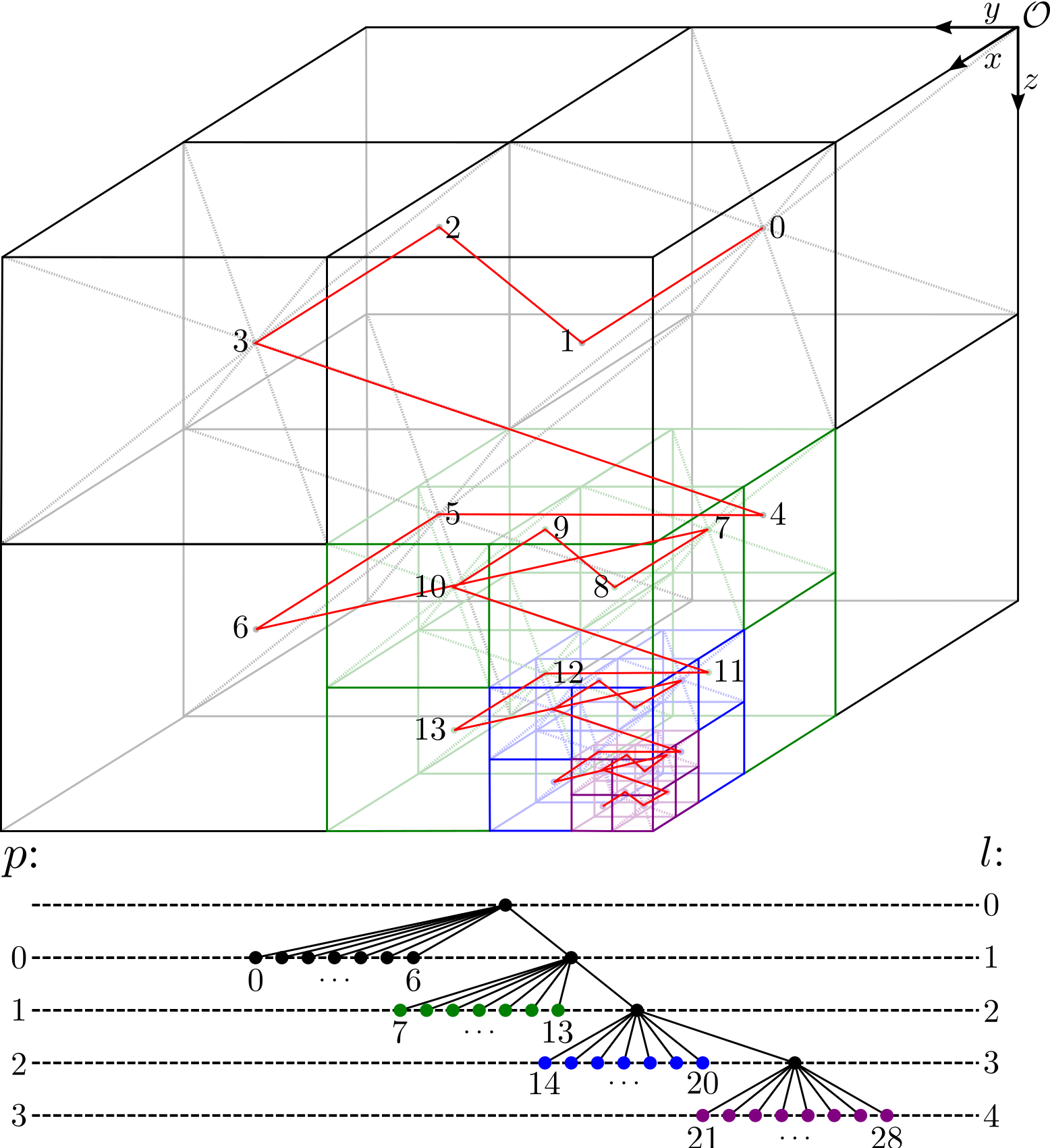
Figure 2: Example of Mesh partitioned and refined by MeshBlock objects indexed via Z-order and traced in red through constituent geometric centroids. The logical relationship between ${}^{p}\Omega_{i}$ and neighbors is stored in an oct-tree. There are no unpopulated leaves. Notice that physical level $p$ and logical level $l$ are distinct; coloring corresponds to physical level: $p=0$ in black, $p=1$ in dark green, $p=2$ in blue, and $p=3$ in purple. (Figure adapted from Daszuta:2021ecf ).

Two main strategies for control over refinement are offered. One may pose that a fixed, region contained within the Mesh is at a desired level $N_{L}$. Alternatively, on individual MeshBlock objects a refinement condition may be imposed. This latter is quite flexible and allows for e.g. time-dependent testing as to whether dynamical fields satisfy some desired criteria. In particular, in the binary-black-hole context, recent work with GR-Athena++ rashti2023adaptivemeshrefinement has compared “box-in-box”, “sphere-in-sphere”, and truncation error estimation as ingredients for the aforementioned condition and the effect on gravitational wave mismatch.

0.2.2 Field discretization

A variety of discretizations of dynamical field components are required to facilitate the evolution of the GRMHD system embedded (§0.3.1) within GR-Athena++. Natively Athena++ supports cell-centered (CC), face-centered (FC), and edge-centered (EC) grids. Thus volume averaged, conserved (primitive) quantities of the Euler equations are taken on CC and suitable mapping to FC (during calculation of e.g. fluxes) leads to a shock-capturing, conservative, Godunov-style finite volume method. When magnetic (electric) fields are present then EC is employed so as to enable use of the Contrained Transport algorithm (see §0.3.3) which preserves the divergence free condition on magnetic fields.

To make the connection to a MeshBlock object concrete, we can first consider the one-dimensional domain $\Omega_{I}:=[a,\,b]$. Grids for uniformly sampled CC and vertex-centers (VC) respectively are:

$$\begin{aligned} \mathcal{G}_{\mathrm{CC}}:=&\Big{\{}a+\Big{(}n+\frac{1}{2}\Big{)}\frac{b-a}{N_{B}}\,\Big{|}\,n\in\{0,\,\dots N_{B}-1\}\Big{\}},\\ \mathcal{G}_{\mathrm{VC}}:=&\Big{\{}a+n\frac{b-a}{N_{B}}\,\Big{|}\,n\in\{0,\,\dots N_{B}\}\Big{\}};\end{aligned}$$ (1)

where $\delta x{}:=(b-a)/N_{B}$ is the grid spacing and $N_{B}$ the sampling parameter. To facilitate communication between MeshBlock objects a thin layer of $N_{\mathrm{g}}{}$ “ghost nodes” (also with spacing $\delta x$) is extended in the direction of each nearest-neighbor MeshBlock. Products of combinations of such grids allow for straight-forward extension to $2^{\mathrm{d}}$ and $3^{\mathrm{d}}$, together with construction of e.g. FC sampling.

For the evolution of purely geometric quantities (induced spatial metric, extrinsic curvature, etc) GR-Athena++ extends the framework by incorporating infrastructure that allows for point-wise description of fields on VC. Our primary motivation for this is one of computational efficiency which may be understood through the following. Consider splitting a fixed $\mathcal{G}_{\mathrm{VC}}$ exactly in half into two new grids each with the same sampling parameter as the parent. This doubles the resolution. We also find that the coarsely spaced parent nodes exactly coincide with interspersed nodes of the children. This behaviour occurs at refinement boundaries (in ghost-layers) for VC sampling due to the $2:1$ ratio nearest-neighbor MeshBlock objects must obey (see §0.2.1). For refinement based on polynomial interpolation this reduces the restriction operation for VC to an injection (copy), and, simplifies prolongation. For a full discussion of our high-order $\mathcal{R}$ and $\mathcal{P}$ for VC see Daszuta:2021ecf .

Geodesic spheres

In GR-Athena++, during simulations, evaluation of diagnostic quantities that are naturally defined as integrals over spherical surfaces is often required. As a particular example we extract gravitational radiation (§0.3.5) through evaluation of numerical quadrature over triangulated geodesic spheres. Using a geodesic grid ensures more even tiling of the sphere compared to the uniform latitude-longitude grid of similar resolution.

A geodesic sphere of radius $R$ (denoted $Q_{R}$) may be viewed as the boundary of a convex polyhedron embedded in $\mathbb{R}^{3}$ with triangular faces, i.e., a simplicial $2$-sphere that is homeomorphic to the $2$-sphere of radius $R$. To construct the geodesic grid we start from a regular icosahedron with 12 vertices and 20 plane equilateral triangular faces, embedded in a unit sphere. This is refined using the so called “non-recursive” approach Wang:2011 . This leads to a polyhedron with $10n_{Q}^{2}+2$ vertices where the refinement parameter $n_{Q}$ controls the so-called grid level. In Fig.3 we show an example of two such grids.

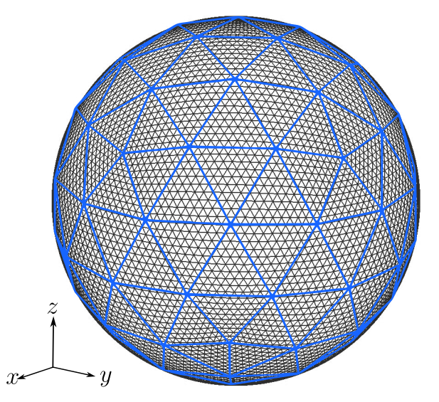
Figure 3: Structure of the geodesic grid used by GR-Athena++. Depicted in light-blue is a grid in consisting of 92 vertices ($n_{Q}=3$). In black we show a grid of 9002 vertices ($n_{Q}=30$); a typical sampling associated with gravitational wave extraction in production simulations.

Note that field data over the Mesh (i.e. local to MeshBlock objects) is treated as independent from a geodesic sphere in our implementation, with transfer achieved via standard Lagrange interpolation.

For evaluation of numerical quadratures we associate to each grid point of a geodesic sphere a solid angle by connecting the circumcenters of any pair of triangular faces that share a common edge. The solid angles subtended by the cells at the center of the sphere are used as weighting coefficients when computing the averages. The logical connection between the neighboring cells is implemented as described in Randall:2002 .

0.3 GRMHD

0.3.1 Dynamical system

Our treatment of GRMHD within GR-Athena++ involves the $\mathrm{Z}4$c system (§0.3.1) coupled to the equations of ideal MHD through matter sources (§0.3.1). The setting of the formulation utilizes the standard geometric view (and definitions) of ADM decomposition Arnowitt:1959ah whereby a space-time manifold endowed with metric $(\mathcal{M},\,g)$ is viewed as foliated by a family of non-intersecting, spatial hypersurfaces with members $\Sigma_{t}$. Fixing notation, recall that one introduces a future-directed $t{}^{a}$ satisfying $t{}^{a}\nabla{}_{a}[t]=1$ and considers $t{}^{a}=\alpha n{}^{a}+\beta{}^{a}$ where $n^{a}$ is a future-directed, time-like, unit normal $n^{a}$ to each member of the foliation $\Sigma{}_{t}$, $\alpha$ is the lapse and $\beta{}^{a}$ the shift. Projections of ambient fields over $\mathcal{M}$ to (various products of) the tangent and normal bundles of $\Sigma$ leads to evolution, and constraint equations. Here we summarise the resulting equations as we have implemented them.

$\mathrm{Z}4$c system

In brief, to stabilize the time-evolution problem, the $\mathrm{Z}4$ formulation Bona:2003fj directly augments the Einstein field equations via suitable introduction of an auxiliary, dynamical vector field $Z^{a}$. This allows for derivation of evolution equations for the induced metric $\gamma{}_{ij}$ on $\Sigma$, the extrinsic curvature $K{}_{ij}:=-\frac{1}{2}\pounds{}_{\mathbf{n}}[\gamma{}_{ij}]$ (with $\pounds{}_{\mathbf{n}}[\cdot]$ the Lie derivative along $n{}^{a}$), and the projected auxiliary quantities $\Theta:=-n{}_{a}Z{}^{a}$ and $\check{Z}_{i}:=\perp^{a}_{i}Z{}_{a}$ (with $\perp^{a}_{b}:=g{}^{a}{}_{b}+n{}^{a}n{}_{b}$).

At its core $\mathrm{Z}4$c Bernuzzi:2009ex ; Hilditch:2012fp is a conformal reformulation featuring constraint damping Gundlach:2005eh ; Weyhausen:2011cg . A further, spatial conformal degree of freedom is factored out:

$$\tilde{\gamma}{}_{ij}:= \psi{}^{-4}\gamma{}_{ij}, \tilde{A}{}_{ij}:= \psi^{-4}\Big{(}K{}_{ij}-\frac{1}{3}K\gamma{}_{ij}\Big{)};$$ (2)

with the trace defined as $K:=K{}_{ij}\gamma{}^{ij}$, and conformal factor $\psi:=(\gamma/f)^{1/12}$ where $\gamma$ and $f$ are determinants of $\gamma{}_{ij}$ and some spatial reference metric $f{}_{ij}$ respectively. It is assumed that $f{}_{ij}$ is flat and in Cartesian coordinates which immediately yields the algebraic constraints:

$$\mathcal{C}_{A}:=\big{(}\ln(\tilde{\gamma}),\,\tilde{\gamma}{}^{ij}\tilde{A}{}_{ij}\big{)}=0.$$ (3)

Additionally we introduce the definitions:

$$\chi:=\gamma{}^{-1/3}, \hat{K}:=K-2\Theta; \tilde{\Gamma}{}^{i}:=2\tilde{\gamma}{}^{ij}\check{Z}{}_{j}+\tilde{\gamma}{}^{ij}\tilde{\gamma}{}^{kl}\partial{}{}_{l}[\tilde{\gamma}{}_{jk}], \widehat{\Gamma}{}^{i}:=\tilde{\gamma}{}^{jk}\tilde{\Gamma}{}^{i}{}_{jk}.$$ (4)

The dynamical variables $\big{(}\chi,\,\tilde{\gamma}{}_{ij},\,\hat{K},\tilde{A}{}_{ij},\,\Theta,\,\tilde{\Gamma}{}^{i}\big{)}$ obey the evolution equations:

$$\partial{}{}_{t}[\chi]= \frac{2}{3}\chi\left(\alpha(\hat{K}+2\Theta)-\partial_{i}[\beta{}^{i}]\right)+\beta{}^{i}\partial_{i}[\chi],$$ (5)

$$\partial{}{}_{t}[\tilde{\gamma}{}_{ij}]=-2\alpha\tilde{A}{}_{ij}+\beta{}^{k}\partial{}_{k}[\tilde{\gamma}{}_{ij}]-\frac{2}{3}\tilde{\gamma}{}_{ij}\partial{}_{k}[\beta{}^{k}]+2\tilde{\gamma}{}_{k(i}\partial{}_{j)}[\beta{}^{k}].$$ (6)

$$\partial{}{}_{t}[\hat{K}]= -\mathrm{D}{}^{i}[\mathrm{D}{}_{i}[\alpha]]+\alpha\left[\tilde{A}{}_{ij}\tilde{A}{}^{ij}+\frac{1}{3}(\hat{K}+2\Theta)^{2}\right]$$

$$+\beta{}^{i}\partial{}{}_{i}[\hat{K}]+\alpha\kappa{}_{1}(1-\kappa{}_{2})\Theta+4\pi\alpha[{}^{~{}A}S+{}^{~{}A}\rho],$$ (7)

$$\partial{}{}_{t}[\tilde{A}{}_{ij}] =\chi[-\mathrm{D}{}_{i}[\mathrm{D}{}_{j}[\alpha]]+\alpha(R{}_{ij}-8\pi{}^{~{}A}S{}_{ij})]^{\mathrm{tf}}+\alpha[(\hat{K}+2\Theta)\tilde{A}{}_{ij}-2\tilde{A}{}^{k}{}_{i}\tilde{A}{}_{kj}]$$

$$\hphantom{=}+\beta{}^{k}\partial{}{}_{k}[\tilde{A}_{ij}]+2\tilde{A}{}_{k(i}\partial{}{}_{j)}[\beta{}^{k}]-\frac{2}{3}\tilde{A}{}_{ij}\partial{}{}_{k}[\beta{}^{k}],$$ (8)

$$\partial{}{}_{t}[\Theta]= \frac{\alpha}{2}\left[\tilde{\mathcal{H}}-2\kappa{}_{1}(2+\kappa{}_{2})\Theta\right]+\beta{}^{i}\partial{}{}_{i}[\Theta],$$ (9)

$$\partial{}{}_{t}[\tilde{\Gamma}{}^{i}]= -2\tilde{A}{}^{ij}\partial{}{}_{j}[\alpha]+2\alpha\Big{[}\tilde{\Gamma}{}^{i}{}_{jk}\tilde{A}{}^{jk}-\frac{3}{2}\tilde{A}{}^{ij}\partial{}{}_{j}[\ln(\chi)]-\kappa{}_{1}(\tilde{\Gamma}{}^{i}-\widehat{\Gamma}{}^{i})$$

$$-\frac{1}{3}\tilde{\gamma}{}^{ij}\partial{}{}_{j}[2\hat{K}+\Theta]-8\pi\tilde{\gamma}{}^{ij}{}^{~{}A}S{}_{j}\Big{]}+\tilde{\gamma}{}^{jk}\partial{}{}_{k}[\partial{}{}_{j}[\beta{}^{i}]]+\frac{1}{3}\tilde{\gamma}{}^{ij}\partial{}{}_{j}[\partial{}{}_{k}[\beta{}^{k}]]$$

$$+\beta{}^{j}\partial{}{}_{j}[\tilde{\Gamma}{}^{i}]-\widehat{\Gamma}{}^{j}\partial{}{}_{j}[\beta{}^{i}]+\frac{2}{3}\widehat{\Gamma}{}^{i}\partial{}{}_{j}[\beta{}^{j}];$$ (10)

where in Eq.(8) the trace-free (tf) operation is computed with respect to $\gamma{}_{ij}$ and $\tilde{\mathcal{H}}$ is defined in Eq.(11). The scalars $\kappa_{1}$ and $\kappa_{2}$ are freely chosen, damping parameters. Definitions of matter fields are standard and based on projections of the decomposed space-time, energy-momentum-stress tensor $T{}_{ab}={}^{A}\rho n{}_{a}n{}_{b}+2{}^{A}S{}_{(a}n{}_{b)}+{}^{A}S{}_{ab}$ in terms of the energy density ${}^{A}\rho:=T{}_{ab}n{}^{a}n{}^{b}$, momentum ${}^{A}S{}_{i}=-T{}_{bc}n{}^{b}\perp^{c}_{i}$, and spatial stress ${}^{A}S{}_{ij}:=T{}_{cd}\perp^{c}_{i}\perp^{d}_{j}$. The intrinsic curvature $R{}_{ij}$ appearing in Eq.(8) is decomposed according to $R{}_{ij}=\tilde{R}^{\chi}{}_{ij}+\tilde{R}{}_{ij}$ where in terms of the connection $\tilde{\mathrm{D}}{}_{i}$ compatible with $\tilde{\gamma}{}_{jk}$:

$$\tilde{R}{}^{\chi}{}_{ij}=\frac{1}{2\chi}\left[\tilde{\mathrm{D}}{}_{i}[\tilde{\mathrm{D}}{}_{j}[\chi]]+\tilde{\gamma}{}_{ij}\tilde{\mathrm{D}}{}^{l}[\tilde{\mathrm{D}}{}_{l}[\chi]]-\frac{1}{2\chi}\tilde{\mathrm{D}}{}_{i}[\chi]\tilde{\mathrm{D}}{}_{j}[\chi]\right]-\frac{3}{4\chi^{2}}\tilde{\mathrm{D}}{}^{l}[\chi]\tilde{\mathrm{D}}{}_{l}[\chi]\tilde{\gamma}{}_{ij},$$

and:

$$\tilde{R}{}_{ij}=-\frac{1}{2}\tilde{\gamma}{}^{lm}\partial{}{}_{l}[\partial{}{}_{m}[\tilde{\gamma}{}_{ij}]]+\tilde{\gamma}{}_{k(i}\partial{}{}_{j)}[\tilde{\Gamma}{}^{k}]+\widehat{\Gamma}{}^{k}\tilde{\Gamma}{}_{(ij)k}+\tilde{\gamma}{}^{lm}(2\tilde{\Gamma}{}^{k}{}_{l(i}\tilde{\Gamma}{}_{j)km}+\tilde{\Gamma}{}^{k}{}_{im}\tilde{\Gamma}{}_{klj}).$$

The dynamical constraints in terms of transformed variables $(\tilde{\mathcal{H}},\,\tilde{\mathcal{M}}{}_{i},\,\Theta,\,\check{Z}{}^{i})$ may be monitored to assess the quality of a numerical calculation:

$$\tilde{\mathcal{H}}:=R-\tilde{A}{}_{ij}\tilde{A}{}^{ij}+\frac{2}{3}\big{(}\hat{K}+2\Theta\big{)}^{2}-16\pi{}^{~{}A}\rho=0,$$ (11)

$$\tilde{\mathcal{M}}{}_{j}:=\tilde{\mathrm{D}}_{i}[\tilde{A}{}^{i}{}_{j}]-\frac{3}{2}\tilde{A}{}^{i}{}_{j}\partial{}_{i}[\ln(\chi)]-\frac{2}{3}\partial{}{}_{j}[\hat{K}+2\Theta]-8\pi{}^{~{}A}S_{j}=0,$$ (12)

$$\Theta= 0, \check{Z}{}^{i}= \tilde{\Gamma}{}^{i}-\widehat{\Gamma}{}^{i}=0.$$ (13)

In order to close the $\mathrm{Z}4$c system we must supplement it with gauge conditions. These are conditions on $(\alpha,\,\beta^{i})$ that in GR-Athena++ are based on Bona-Másso lapse Bona:1994b and the gamma-driver shift Alcubierre:2002kk :

$$\partial_{t}[\alpha] =-\mu{}_{L}\alpha^{2}\hat{K}+\beta{}^{i}\partial_{i}[\alpha], \partial_{t}[\beta{}^{i}] =\mu{}_{S}\alpha^{2}\tilde{\Gamma}{}^{i}-\eta\beta{}^{i}+\beta{}^{j}\partial{}_{j}[\beta{}^{i}].$$ (14)

In specification of Eq.(14) we employ the $1+\log$ lapse variant $\mu{}_{L}=2/\alpha$ together with $\mu{}_{S}=1/\alpha{}^{2}$. The $\eta$ term serves as a free damping parameter.

MHD and coupling

In order to couple to the $\mathrm{Z}4$c system of §0.3.1 consider the energy-momentum-stress (EMS) tensor factored into perfect fluid and electromagnetic parts:

$$T{}^{\mu\nu}=\Big{[}\rho hu{}^{\mu}u{}^{\nu}+pg{}^{\mu\nu}\Big{]}+\Big{(}b{}^{2}u{}^{\mu}u{}^{\nu}+\frac{1}{2}b^{2}g{}^{\mu\nu}-b{}^{\mu}b{}^{\nu}\Big{)}.$$ (15)

Focusing on the perfect fluid sector (first bracketed term) we have fluid quantities $u{}^{\mu}$, $\rho$, $p$, $h:=1+\epsilon+p/\rho$, and $\epsilon$, which are respectively a time-like velocity 4-vector, rest mass density, pressure, relativistic specific enthalpy, and specific internal energy. Write $u{}^{\mu}=(u{}^{0},u{}^{i})$ and define spatial components of the fluid $4$-velocity by forming the projection to $\Sigma_{t}$ as:

$$\tilde{u}{}^{i}=\bot{}^{i}_{\mu}u{}^{\mu}=u{}^{i}+\frac{W\beta{}^{i}}{\alpha},$$ (16)

where $W:=-n{}_{\mu}u{}^{\mu}$ is the Lorentz factor between Eulerian and comoving fluid observers. This leads to the fluid $3$-velocity $v{}^{i}:=\tilde{u}{}^{i}/W$ and $\tilde{v}{}^{i}:=v{}^{i}-\beta{}^{i}/\alpha$. The second bracketed term of Eq.(15) carries the electromagnetic contribution. The terms $b{}^{\mu}$ and $b^{2}$ appearing there describe the magnetic field and arise as projections of the dual Faraday tensor along $u{}^{\mu}$. Recall that with respect to Eulerian observers the magnetic $\mathcal{B}^{\mu}$ and electric field $\mathcal{E}^{\mu}$ can be used to express the Faraday tensor as:

$$F{}^{\mu\nu}=n{}^{\mu}\mathcal{E}{}^{\nu}-\mathcal{E}{}^{\mu}n{}^{\nu}-\epsilon{}^{\mu\nu\rho\sigma}n{}_{\rho}\mathcal{B}{}_{\sigma},$$

and $\epsilon^{\mu\nu\rho\sigma}$ is the 4 dimensional Levi-Civita pseudo-tensor. Define the dual tensor ${}^{*}F{}^{\mu\nu}:=\frac{1}{2}\epsilon{}^{\mu\nu\rho\sigma}F{}_{\rho\sigma}$. Projecting as $b{}^{\mu}=u{}_{\nu}{}^{*}F{}^{\mu\nu}$ leads to:

$$b{}^{0} =\frac{W\mathcal{B}{}^{i}v{}_{i}}{\alpha}, b{}^{i} =\frac{\mathcal{B}{}^{i}+\alpha b{}^{0}W\tilde{v}{}^{i}}{W}, b{}^{2} =g{}_{\mu\nu}b{}^{\mu}b{}^{\nu}=\frac{(\alpha b{}^{0})^{2}+\mathcal{B}{}^{i}\mathcal{B}{}^{j}\gamma{}_{ij}}{W^{2}}.$$

We form evolution equations for MHD as a balance (conservation) law as in Banyuls:1997zz :

$$\partial{}_{t}\mathbf{q}+\partial{}_{i}\mathbf{F}^{i}=\mathbf{s},$$ (17)

where the conservative variables $\mathbf{q}$ are associated to the Eulerian observer. In our convention $\mathbf{q}:=(D,S_{j},\tau,B^{k})$. Note that we take as primitive variables $\mathbf{w}=(\rho,\tilde{u}^{i},p,B^{i})$ and may map to $\mathbf{q}$ through:

$$\mathbf{q}=\sqrt{\gamma}\left(\rho W,(\rho h+b^{2})W\tilde{u}{}_{j}-\alpha b{}^{0}b{}_{j},(\rho h+b^{2})W^{2}-\rho W-\left(p+\frac{b^{2}}{2}\right)-(\alpha b{}^{0})^{2},\mathcal{B}{}^{k}\right).$$

The inversion of this map, where required, is evaluated numerically (§0.3.4).

In order to determine the flux vector $\mathbf{F}{}^{i}$, and source $\mathbf{s}$ of Eq.(17) one considers the conservation of rest mass density $\nabla{}_{\mu}[\rho u{}^{\mu}]=0$, the Bianchi identity $\nabla{}_{\mu}[T{}^{\mu\nu}]=0$, and the Maxwell relation $\nabla{}_{\mu}[{}^{*}F{}^{\mu\nu}]=0$. The former two equations are projected onto and normal to $\Sigma_{t}$ whereas the latter is projected onto $\Sigma_{t}$. This results in:

$$\mathbf{F}^{i}=\begin{bmatrix}&D\alpha\tilde{v}^{i}\\ &S_{j}\alpha\tilde{v}^{i}+\delta^{i}_{j}\left(p+\frac{b^{2}}{2}\right)\alpha\sqrt{\gamma}-\frac{\alpha\sqrt{\gamma}b_{j}\mathcal{B}^{i}}{W}\\ &\tau\alpha\tilde{v}^{i}+\alpha\sqrt{\gamma}\left(\left(p+\frac{b^{2}}{2}\right)v^{i}-\frac{\alpha b^{0}\mathcal{B}^{i}}{W}\right)\\ &\alpha(B^{k}\tilde{v}^{i}-B^{i}\tilde{v}^{k})\end{bmatrix}.$$ (18)

and:

$$\mathbf{s}=\alpha\sqrt{\gamma}\begin{bmatrix}&0\\ &T^{00}\left(\frac{1}{2}\beta^{i}\beta^{k}\partial{}_{j}\gamma_{ik}-\alpha\partial{}_{j}\alpha\right)+T^{0i}\beta^{k}\partial{}_{j}\gamma_{ik}+T^{0}_{i}\partial{}_{j}\beta^{i}+\frac{1}{2}T^{ik}\partial{}_{j}\gamma_{ik}\\ &T^{00}\left(\beta^{i}\beta^{j}K_{ij}-\beta^{i}\partial{}_{i}\alpha\right)+T^{0i}\left(2\beta^{j}K_{ij}-\partial{}_{i}\alpha\right)+T^{ij}K_{ij}\\ &0^{k}\end{bmatrix}.$$

One further projection can be formed. The Maxwell relation when projected in the normal direction to $\Sigma_{t}$ gives rise to the divergence-free constraint on $B{}^{i}$, that is $\partial{}_{i}[B{}^{i}]=0$. This will be automatically enforced by the discretisation of the equations (§0.3.3). Finally, the MHD equations are coupled to the $\mathrm{Z}4$c system (0.3.1) through the the ADM sources (here prefixed with superscript $A$):

$$\begin{gathered}\begin{aligned} {}^{A}\rho=&(\rho h+b^{2})W^{2}-\left(p+\frac{b^{2}}{2}\right)-(\alpha b{}^{0})^{2},\\ {}^{A}S{}_{i}=&(\rho h+b^{2})W^{2}v{}_{i}-b{}^{0}b{}_{i}\alpha,\\ {}^{A}S{}_{ij}=&(\rho h+b^{2})W^{2}v{}_{i}v{}_{j}+\left(p+\frac{b^{2}}{2}\right)\gamma{}_{ij}-b{}_{i}b{}_{j}.\end{aligned}\end{gathered}$$ (19)

0.3.2 Equation of state

The GRMHD system of conservation laws together with the magnetic field divergence-free condition restricts $8$ degrees of freedom for the $9$ primitive variables $(\rho,p,\epsilon,\tilde{u}^{i},B^{i})$. The role of the equation of state (EOS) is to reduce this underdeterminedness through imposition of a thermodynamical relationship.

Here we highlight two classes of EOS used in GR-Athena++:

1. Ideal gas with Gamma-law: A relation between $(\rho,p,\epsilon)$ is formed with $p=\rho\epsilon(\Gamma-1)$ imposed where $\Gamma=1+1/n$ and $n$ is the adiabatic index of the fluid. During initialisation this is supplemented by the barotropic relation $p=K\rho^{\Gamma}$ where $K$ serves as a problem-dependent, fluid mass-scale.

2. Tabulated, 3-dimensional finite-temperature: First, species fractions $Y_{i}$ that track fluid composition are introduced (CMA scheme Plewa:1998nma ). For simplicity, consider only the electron fraction $Y_{\mathrm{e}}$. This extra variable is incorporated into the GRMHD system as an additional evolved variable $DY_{e}$ with zero source. Overall this allows us to write the relation $p=p\left(\rho,T,Y_{\mathrm{e}}\right)$. Quantities $\rho$ and $T$ are tabulated in logarithmic space, and, together with $Y_{\mathrm{e}}$ are linearly interpolated so as to provide $\log p$ when required.

   Our implementation supports tables in the form used by the CompOSE database Typel:2013rza processed to also include the sound speed by the PyCompOSE tool .

0.3.3 Numerical technique

In treatment of the GRMHD system in GR-Athena++ the method of lines approach is taken. In this overview attention is restricted to time-evolution based on the third order, three stage, low-storage SSPRK$(3,3)$ method of gottlieb2009highorderstrong .

Field components involved in the $\mathrm{Z}4$c sub-system (§0.3.1) are sampled on vertex-centers (VC). Spatial derivatives on the interior of the computational domain $\mathrm{int}(\Omega)$ (i.e. in the bulk away from $\partial\Omega$) are computed with high-order, centered, finite difference (FD) stencils with one-point lop-siding for advective terms (see e.g.Brugmann:2008zz ). The ghost-layer extent (choice of $N_{\mathrm{g}}$) fixes the overall, formal FD approximation order as $2(N_{\mathrm{g}}-1)$ throughout $\mathrm{int}(\Omega)$. The interpolation order during calculation of $\mathcal{P}$ under mesh refinement is consistently selected to match that of the FD; whereas $\mathcal{R}$ is exact for VC.

To fix physical boundary conditions, within every time-integrator sub-step, an initial Lagrange extrapolation (involving $N_{\mathrm{g}}+1$ points) is performed so as to populate a ghost-layer at $\partial\Omega$. The dynamical $\mathrm{Z}4$c equations then furnish data for $\{\chi,\,\tilde{\gamma}{}_{ij},\,\alpha,\,\beta{}^{i}\}$ at $\partial\Omega$ whereas values there for $\{\hat{K},\,\tilde{\Gamma},\,\Theta,\,\tilde{A}{}_{ij}\}$ are based on the Sommerfeld prescription of Hilditch:2012fp .

During evolution the Courant-Friedrich-Lewy (CFL) condition must be satisfied. In the context of (GR-)Athena++ grid-spacing on the most refined level of a refinement hierarchy determines the global time-step that is applied on each MeshBlock. Finally for the evolved $\mathrm{Z}4$c state-vector, high-order Kreiss-Oliger (KO) dissipation Kreiss:1973 , of degree $2N_{\mathrm{g}}{}$, with uniform factor $\sigma_{D}{}$ is applied.

In the case of the MHD sub-system (§0.3.1) a standard conservative, Godunov-style finite volume method is employed. Thus, practically, when the conserved variables $\mathbf{q}$ are to be evolved, we require fluxes (Eq.(18)) evaluated at cell interfaces. Interface data is prepared based on reconstruction of known cell-averaged quantities to the left and right of an interface. Once prepared we can utilize e.g. Local-Lax-Friedrichs (LLF):

$$\hat{\mathbf{F}}_{i+1/2}=\frac{1}{2}\left(\mathbf{F}[\mathbf{q}^{-}_{i+1/2}]+\mathbf{F}[\mathbf{q}^{+}_{i-1/2}]-\alpha(\mathbf{q}^{+}_{i-1/2}-\mathbf{q}^{-}_{i+1/2})\right),$$

where $\alpha$ is taken as the maximum over characteristic speeds, which, are computed from locally reconstructed variables, while we note the availability of more sophisticated Riemann solvers for magnetic fields such as those presented in Kiuchi:2022ubj . In the absence of magnetic fields exact characteristic speeds are provided in Banyuls:1997zz whereas for MHD we follow the approximate prescription of Gammie:2003rj . In the MHD context preservation of the magnetic field divergence-free condition requires some care. This is achieved through a constrained transport scheme which we return to in §0.3.3.

Intergrid transfer, and reconstruction

In (GR-)Athena++, data transfer between differing discretizations for the evolved field components of GR and MHD is required at various points of the time-evolution algorithm. Indeed CC grids form the primary representation for the evolved, conserved quantities $\mathbf{q}$, furthermore the FC and EC grids are utilized for constrained transport. The (smooth) geometric data is evolved on VC. For simplicity, this latter, is transferred to the other grids, as required, at linear order.

In order to evaluate the numerical fluxes at the cell interfaces, we reconstruct the primitive variables $\mathbf{w}$ from CC to FC. Reconstruction avoids the increase of total variation, providing a limited interpolation strategy appropriate for functions of locally reduced smoothness. To this end the Piecewise Linear Method (PLM) vanLeer:1974a , and Piecewise Parabolic Method (PPM) Colella:2011a ; McCorquodale:2015a , as implemented in Athena++, are further supplemented in GR-Athena++ by WENO5 Jiang:1996a and WENOZ Borges:2008a .

Constrained transport

The ideal MHD approximation reduces the Maxwell equations to a hyperbolic equation for the magnetic field components, the induction equation, and an elliptic equation, Gauss’s Law. The solution of this elliptic equation at each time-step in a numerical simulation through e.g. a relaxation method would be incredibly costly and so various schemes have been developed to avoid this requirement, as discussed above. Athena++ employs an implementation of the constrained transport approach to ensure divergence free evolution of the magnetic field, following the original proposal of Evans:1988a , with the development of the specific implementation in Athena++ following Gardiner:2005 ; Gardiner:2007nc ; Stone:2008mh ; Beckwith:2011iy ; White:2015omx .

Here the magnetic field is discretised, not as a cell average as for the other hydrodynamical variables, or as in other implementations such as the Flux-CT implementation of Toth:2000 , but as face averages:

$$B^{x}_{i-1/2,j,k}=\frac{1}{\Delta A}\int_{A_{i-1/2,j,k}}B^{x}\mathrm{d}y\mathrm{d}z,$$ (20)

with the other components $B^{y},B^{z}$ discretised on, respectively, the $y$ and $z$ faces of the computational cell $A_{i,j-1/2,k}$, $A_{i,j,k-1/2}$, with $\Delta A$ the area of the face being integrated over.

Noting that the electric field is given by the cross product of the magnetic field with the fluid velocity $\alpha\tilde{v}$, integrating the induction equation over a face of the computational cell gives an evolution equation for the face averaged magnetic field in terms of the integrated curl of the electric field over the face. By applying Stokes theorem, the face centred magnetic field is updated by evaluation of the integral of the edge centred, time averaged, electric field around the face in question:

$$\int^{t_{n+1}}_{t_{n}}\partial_{t}B^{x}_{i-1/2,j,k}\mathrm{d}t = \frac{1}{\Delta A}\int^{t^{n+1}}_{t^{n}}\mathrm{d}t\int_{A_{i-1/2,j,k}}\Big{\{}-\partial_{y}(\alpha(B^{x}\tilde{v}^{y}-B^{y}\tilde{v}^{x}))$$

$$-\partial_{z}(\alpha(B^{x}\tilde{v}^{z}-B^{z}\tilde{v}^{x}))\mathrm{d}y\mathrm{d}z\Big{\}},$$

$$= \frac{1}{\Delta A}\int^{t^{n+1}}_{t^{n}}\mathrm{d}t\int_{A_{i-1/2,j,k}}-\partial_{y}(E^{z})+\partial_{z}(E^{y})\mathrm{d}y\mathrm{d}z,$$

$$B^{x,n+1}_{i-1/2,j,k} = B^{x,n}_{i-1/2,j,k}-\frac{\Delta t}{\Delta A}\int_{\partial A_{i-1/2,j,k}}\mathbf{E}^{n+1/2}\cdot\mathbf{\mathrm{d}l},$$ (21)

where $\mathbf{\mathrm{d}l}$ is the line element around the edge of face $A_{i-1/2,j,k}$, and $\mathbf{E}^{n+1/2}$ the time averaged electric field between $t_{n}$ and $t_{n+1}$.

It is clear that this discretisation of the field automatically preserves the divergence of $B$ between time-steps; when evaluating the divergence of $B^{n+1}$ using the above expression, contributions from the electric field will cancel due to shared edges between faces having opposite signs due to the orientations of the integrals around the face edges. The divergence of $B^{n+1}$ must then equal the divergence of $B^{n}$.

The final requirement for evaluating the magnetic field is to calculate the time averaged, edge centred, electric fields.

Following the standard Godunov approach, the time averaged face centred electric field can be calculated as the solution to the Riemann problem at the cell interface, which is calculated along with the hydrodynamical fluxes. Then the cell centred electric field can be explicitly constructed as the cross product of the magnetic field and fluid 3-velocity. The derivative of the electric field from the cell centre to face centre can be calculated, and then upwinded to the cell face in the upwind direction as determined by the sign of the mass flux. This gradient is then used to integrate the time averaged face centred electric field to the cell edge.

A detailed description of this procedure may be found in White:2015omx , though we note that the implementation for dynamical space-times requires the appropriate densitisation of variables by the time dependent metric determinant, which can no longer be factored out of time derivatives.

For simulations with AMR new MeshBlocks will be created dynamically, on which data will be populated through interpolation from the coarser (finer) MeshBlock(s) that they replace. Naively, this interpolation will not respect the divergence free constraint on $B$, and so Athena++ implements the restriction and prolongation operators of Toth:2002a designed to preserve the curl and divergence of interpolated vector fields.

At the interface between refinement levels, faces and edges of MeshBlocks of different levels overlap. To ensure a conservative evolution the face centred hydrodynamical fluxes are kept consistent, by replacing the face centred flux on the coarser block with the area weighted sum of the fluxes on the finer blocks. Similarly for the magnetic field evolution, the edge centred electric field on the coarser block is replaced with the length weighted sum of the edge centred fields on the finer block. To ameliorate other effects such as the non-deterministic order of MPI processes, shared edge centred electric fields are replaced by their averages also in the case of neighboring MeshBlocks on the same refinement level.

0.3.4 Conservative-to-primitive variable inversion

In order to evaluate the fluxes in Eq. (17) we convert the conservative variables, $\mathbf{q}$ to their primitive representation $\mathbf{w}$ by inverting the definitions of $\mathbf{q}$ in Eq. (18). This involves solution of a non-linear system for the primitive variables. To this end GR-Athena++ features a custom, error-policy based implementation PrimitiveSolver. We have also coupled the external library RePrimAnd of Kastaun:2020uxr . Here we note some additional considerations related to the latter method. Generically the conservative-to-primitive inversion is evaluated pointwise, where required, over a MeshBlock, though is not subject to the underlying particulars in choice of discretization.

Physically we expect a neutron-star (NS) to have a well defined, sharp surface. Consider a radial slice of the fluid density from the NS center: a non-negative profile that drops to zero is expected. Resolving such sharp features can lead to numerical issues during the variable conversion process. In order to address this we follow the standard technique of introducing a tenuous atmosphere region where primitive variables are set according to:

$$\rho_{\mathrm{atm}} =f_{\mathrm{atm}}\rho_{\mathrm{max}}, p_{\mathrm{atm}} =p(\rho_{\mathrm{atm}}), \tilde{u}^{i}_{\mathrm{atm}} =0;$$ (22)

with $\rho_{\mathrm{max}}$ the maximum value of the fluid density in the initial data, and $f_{\mathrm{atm}}$ a problem-specific parameter. The magnetic field is left unaltered in the atmosphere. During the course of the evolution, physical processes of the star, or numerical dissipation, may drive the fluid into the atmosphere region. On account of this we impose an additional criterion where if $\rho<\rho_{\mathrm{thr}}=f_{\mathrm{thr}}\rho_{\mathrm{atm}}$ the cell is reset to atmosphere. Similarly cells are reset to atmosphere if conversion from conservative to primitive variables fails to converge. When atmosphere values are set, we recalculate the conservative variables from the atmosphere primitives and metric variables.

0.3.5 Diagnostic quantities

For later convenience common scalar diagnostic quantities computed during simulations are collected here.

Energetics

The baryon mass is a conserved quantity defined as:

$$M_{b}=\int_{\Sigma_{t}}D{\rm d}^{3}x;$$ (23)

where the integral is evaluated over the entire computational domain. Various energy contributions to the GRMHD system are similarly evaluated:

$$E_{\rm Kin} =\frac{1}{2}\int_{\Sigma_{t}}\frac{S_{i}S^{i}}{D}{\rm d}^{3}x, E_{B} =\frac{1}{2}\int_{\Sigma_{t}}\sqrt{\gamma}Wb^{2}{\rm d}^{3}x, E_{\rm int} =\int_{\Sigma_{t}}D\epsilon{\rm d}^{3}x.$$ (24)

Gravitational wave extraction

To obtain the gravitational wave (GW) content of the space-time, we calculate the Weyl scalar $\Psi_{4}$, the projection of the Weyl tensor onto an appropriately chosen null tetrad $k,l,m,\bar{m}$ with the conventions of Brugmann:2008zz . Multipolar decomposition onto spin-weighted spherical harmonics ${}_{s}Y_{lm}$ of spin-weight $s=-2$ is evaluated through:

$$\psi_{\ell m} = \int^{2\pi}_{0}\int^{\pi}_{0}\Psi_{4}\,\bar{{}_{-2}Y_{\ell m}}(\vartheta,\,\varphi)\sin\vartheta\mathrm{d}\vartheta\mathrm{d}\varphi.$$ (25)

Thus $\Psi_{4}$ is first calculated at all grid points throughout the Mesh whereupon data is interpolated onto a set of geodesic spheres $Q_{R}$ (see §0.2.2) at given extraction radii $R_{Q}$. Subsequently the numerical quadrature of Eq.(25) may be evaluated. In order to select the grid level parameter $n_{Q}$ that controls the number of samples on $Q_{R}$ we may match the area element to that of any intersected MeshBlock objects through $n_{Q}=\left\lceil\sqrt{\frac{\pi R_{Q}^{2}}{\delta x^{2}}-2}\right\rceil$. The modes of the GW strain $h$ may be computed from the projected Weyl scalar by integrating twice in time $\psi_{\ell m}=\ddot{h}_{\ell m}$. The strain is then given by the mode-sum:

$$h_{+}-ih_{\times}=\frac{G}{D_{L}}\sum_{\ell=2}^{\infty}\sum_{m=-\ell}^{\ell}h_{\ell m}(t)\;{}_{-2}Y_{\ell m}(\vartheta,\varphi)\,,$$ (26)

where $D_{L}=(1+z)R$ is the luminosity distance of a source located at distance $R$ to the observer and at redshift $z$. Phase and frequency conventions follow the LIGO algorithms library lalsuite .

0.3.6 Task-list execution model

The individual components of a calculation during a time-evolution sub-step that must be executed must satisfy a particular order of execution. The task-based execution model employed in (GR-)Athena++ may be viewed as assembling this information in a directed, acyclic graph (DAG). A task specifies a given operation that must be performed and may feature dependency on the prior completion of other tasks. These may be assembled so as to represent a more complicated calculation into a so-called task-list. This allows to neatly encapsulate the calculation steps involved in GRMHD in Fig.4.

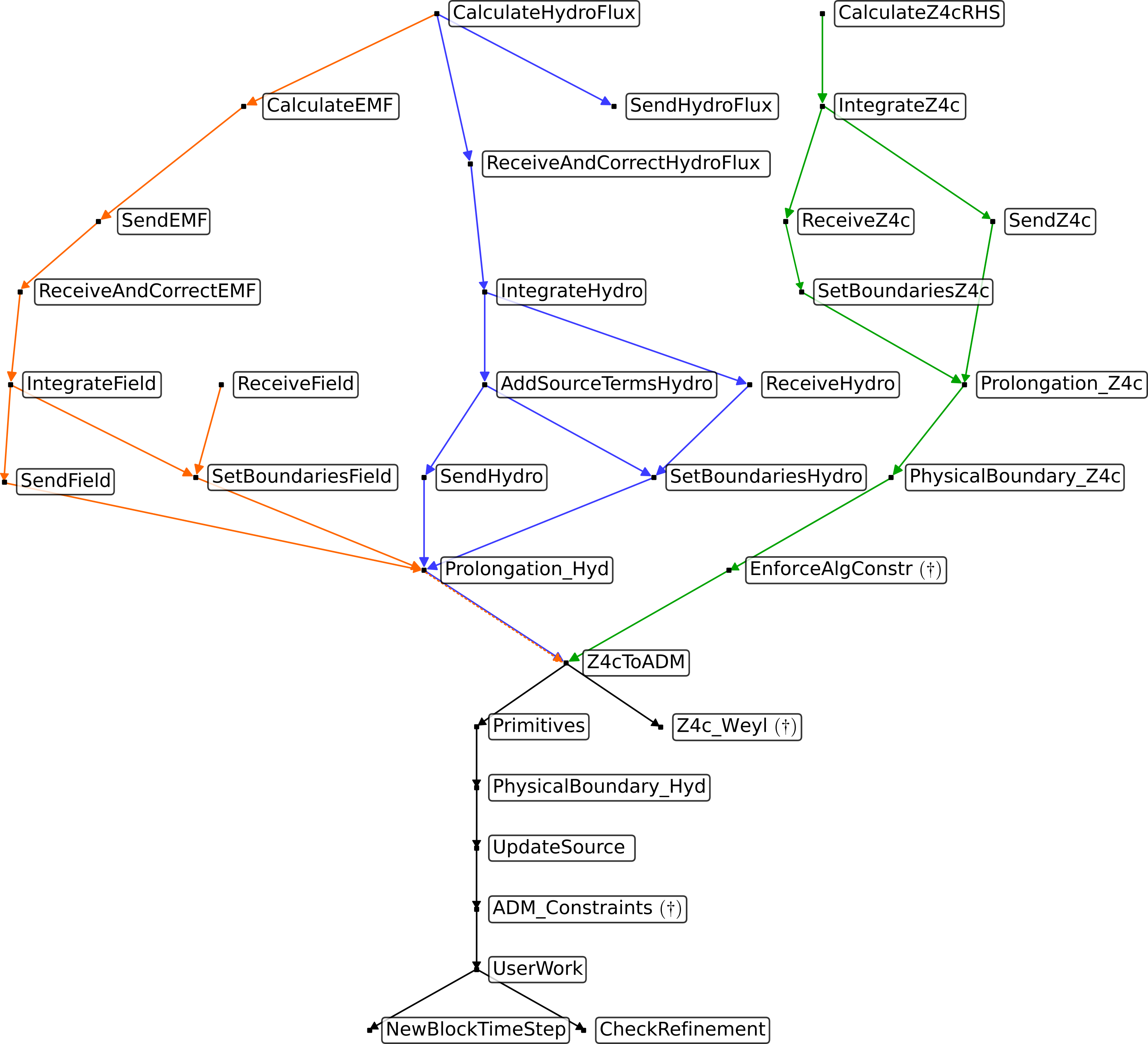
Figure 4: Simplified DAG of GRMHD task-list in GR-Athena++ executed on each MeshBlock during a time-integrator sub-step. Tasks are boxed and arrows between nodes indicate direction of dependency. In the absence of a dependency, remaining tasks may be executed in parallel. Labels indicate operation being performed. Arrows are color-coded according to type of field data manipulated where: (orange) corresponds to magnetic field; (blue) fluid; (green) $\mathrm{Z}4$c; (black) general operations. Tasks labeled with a $(\dagger)$ are only executed on the final integrator sub-step.

One advantage of this form of calculation assembly is that wait time during buffer-communication can be masked as e.g. system calculations proceed in parallel, this feature improves efficiency. Thus, for example, as shown in Fig.4 once the CalculateZ4cRHS and IntegrateZ4c tasks are completed on the current MeshBlock a suitable subset of this data may be sent via communication buffers (SendZ4c task) to a nearest-neighbor MeshBlock so as to populate its ghost-layer (and vice-versa through the RecvZ4c task). Once these tasks complete, boundary data on the current MeshBlock may be set as represented by SetBoundariesZ4c and prolongated where required. As a final note, operations involving global data reduction (e.g. numerical quadrature over geodesic sphere in gravitational wave calculation §0.2.2) are performed external to the task-list.

0.4 Applications

We now demonstrate the performance and accuracy of GR-Athena++ through solution of problems in dynamical space-times with GRMHD. A subset of tests based on our work Cook:2023bag is summarised for NS space-times, followed by a set of first applications, in the long term study of magnetic field development in an isolated NS, and in using AMR to efficiently study the Kelvin-Helmholtz instability during a BNS merger.

Throughout this discussion $N_{\mathrm{g}}{}=4$ is selected which sets $6^{\mathrm{th}}$ order accurate finite differencing in treatment of $\mathrm{Z}4$c. Damping parameters are taken as $\kappa_{1}=0.02$, and $\kappa_{2}=0$. Kreiss-Oliger dissipation is fixed at $\sigma_{D}{}=0.5$.

0.4.1 Single Star Spacetimes

GRHD evolution of Static Neutron Star

Our first test is of the evolution of a static NS model known as A0 in the convention of Dimmelmeier:2005zk , commonly used as a code benchmark, e.g. Font:2001ew ; Thierfelder:2011yi . The star has baryon mass $M_{b}=1.506{\rm M_{\odot}}$ and gravitational mass $M=1.4{\rm M_{\odot}}$, with initial data calculated by solving the Tolman-Oppenheimer-Volkoff (TOV) equations using a central rest-mass density of $\rho_{c}=7.905\times 10^{14}{\rm g\,cm^{-3}}$, with an ideal gas EOS with $\Gamma=2$, and initial pressure set using the polytropic EOS with $K=100$.

Our grid configuration has outer boundaries at $[\pm 378.0,\pm 378.0,\pm 378.0]$ km, with 6 levels of static mesh refinement fully covering the star, with the innermost level covering the region $[\pm 14.8,\pm 14.8,\pm 14.8]$ km. The grid resolution is set through the Mesh parameter $N_{M}=32,48,64,128$, which gives a grid spacing of $[369,246,185,92.3]$ m on the finest level.

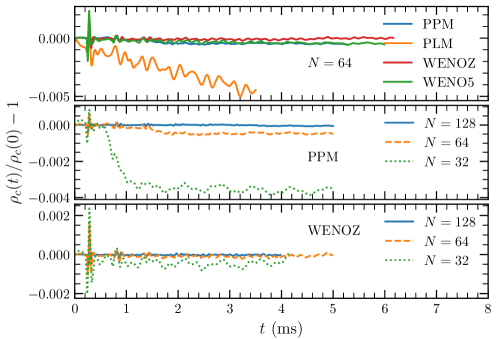
Figure 5: GRHD Evolution of central rest-mass density of the static star A0 model. Top: varying reconstruction at constant resolution $N_{M}=64$. Central, Bottom: varying resolution for PPM and WENOZ reconstruction respectively. Note: Some data has been truncated to $5$ ms for ease of visualisation. (Figure adapted from Cook:2023bag ).

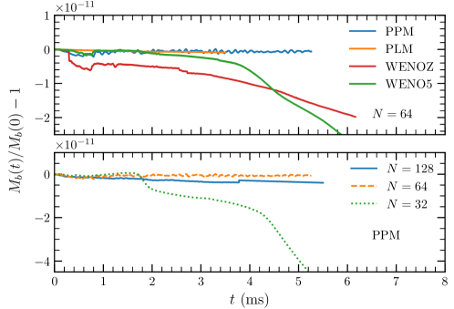
Figure 6: Baryon mass conservation during evolution of the static star A0 model. The mass conservation can be violated due to the artificial low-density atmosphere as the fluid expands beyond the computational domain. (Figure adapted from Cook:2023bag ).

We first demonstrate the evolution of the central rest mass density of the star $\rho_{c}(t)$ as a function of resolution and for a variety of reconstruction schemes in Fig. 5. The star is perturbed by the presence of truncation errors, leading to the excitation of characteristic oscillations in the central density, the frequencies of which match those predicted by perturbation theory for the first three radial modes, at frequencies of $\nu_{F}=1462,3938$ and $5928$ Hz Baiotti:2008nf , and the relative amplitudes of which remain below $10^{-2}$, and converge away as resolution increases. We find that, as expected, PLM is the least accurate scheme, with PPM performing poorly at low resolutions, but performing consistently with WENO schemes at higher resolutions.

In Fig. 6 we demonstrate a relative conservation of baryon mass at the level of $10^{-11}$ consistently across schemes and resolutions, with violations occuring due the setting of atmosphere levels and matter leaving the computational domain. The best performance is found for PPM, which preserves the star surface most accurately.

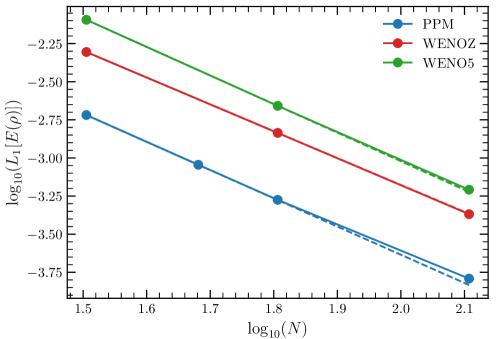
Figure 7: Convergence of $L_{1}[E(\rho)]:=|\rho(\mathbf{x},t)-\rho(\mathbf{x},0)|$ for static star model A0 at $t=2.96$ ms. Order of convergence is $1.85,1.76,1.87$ for PPM, WENOZ, WENO5 reconstruction schemes respectively. (Figure adapted from Cook:2023bag ).

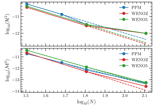
Figure 8: Hamiltonian (top) and momentum (bottom) constraints for static star model A0 at $t=2.96$ ms. Order of convergence in the Hamiltonian (momentum) constraint is $3.51(4.41),3.65(5.46),3.64(4.88)$ for PPM, WENOZ, WENO5 respectively. (Figure adapted from Cook:2023bag ).

The convergence of three, spatially integrated, quantities is demonstrated for this model: the absolute difference between the density profile at time $t$ and the initial density profile; and the Hamiltonian and Momentum constraints (§0.3.1). We show the former in Fig. 7, with dashed lines showing linear extrapolations from the first two data points, the slopes of which indicate the order of convergence. Approximately $2^{\mathrm{nd}}{}$ convergence is found, most clearly seen in the WENO(5,Z) schemes, while at the resolutions shown the PPM scheme has the lowest overall error. In Fig. 8, the constraints are shown to converge at an order between 3.51 and 5.46 depending on the reconstruction scheme used.

Long-term Magnetic field dynamics in Static Neutron Star

We now present an application of GR-Athena++ to the long term evolution of magnetic fields within NSs. The existence of a magnetic field configuration that is stable over long timescales within a NS is an open problem, with analytic and numerical studies showing the instability of purely poloidal fields on Alfven timescales, and suggesting the need for the development of a toroidal component to stabilise the field Tayler:1957a ; Tayler:1973a ; Wright:1973a ; Markey:1973a ; Markey:1974a ; Flowers:1977a ; Braithwaite:2005md , with long term numerical relativity evolutions necessary to understand the rearrangement of the field profile and energy distribution Kiuchi:2008ss ; Lasky:2011un ; Ciolfi:2011xa ; Pili:2017yxd ; Sur:2021awe .

We evolve an isolated star given by model A0, using WENOZ reconstruction, the grid set up of §0.4.1 and resolutions $N_{M}=32,64,128$, with a purely poloidal field given by  Liu:2008xy :

$$(A_{x},A_{y},A_{z})=(-yA_{\varphi},xA_{\varphi},0),$$ (27a)

$$A_{\varphi}:=A_{b}\max(p-0.04\,p_{\rm max},0).$$ (27b)

where $p_{\mathrm{max}}$ is the maximum value of the pressure within the star.

The magnetic field is given by $B=\nabla\times A$, with $A_{b}$ a free parameter scaling the overall strength of the field. Below we set this so that the maximum value of the magnetic field inside the star is $1.84\times 10^{16}$ G, approximately the magnetic field strength expected in magnetars.

We compare our results with our earlier simulations of a similar system, performed in the Cowling approximation in Sur:2021awe .

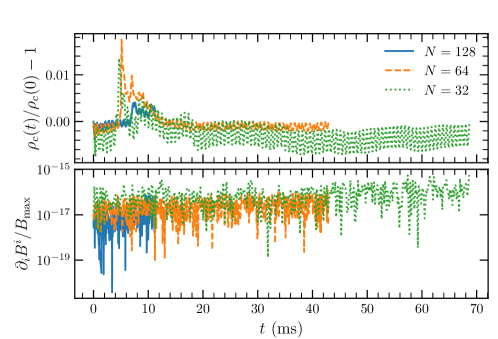
Figure 9: Top: Evolution of central rest-mass density of the static star A0 model with superposed poloidal magnetic field, and WENOZ reconstruction. Bottom: $\partial_{i}B^{i}$ integrated over full computational domain $\Omega$ and normalised by $B_{\mathrm{max}}:=\max_{\Omega}B$. (Figure adapted from Cook:2023bag ).

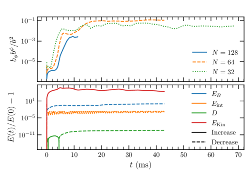
Figure 10: Top: Growth of the toroidal component of magnetic field energy as a fraction of the total for model shown in Fig.9. Bottom: relative change in magnetic energy, internal energy, mass and kinetic energy for $N_{M}=64$. Solid lines denote a positive change in energy, dashed lines denote a negative change. (Figure adapted from Cook:2023bag ).

We first demonstrate the oscillations of the central density of the star in the upper panel of Fig. 9. In comparison to the case in the absence of magnetic fields (Fig. 5) we see larger oscillations, driven by the superposed $B$-field. We see the peak in oscillations corresponds to the saturation time of the toroidal field compoenent growth. Throughout the evolution the constrained transport algorithm maintains the divergence free condition on the magnetic field with a relative violation of ${{\sim}10^{-16}}$ shown in the lower panel of Fig. 9.

As expected we see a growth of a toroidal field component to stabilise the poloidal component, shown in the upper panel of Fig. 10. After $\sim{}16$ ms, the ratio of toroidal to total magnetic field energy $b^{\phi}b_{\phi}/b^{\mu}b_{\mu}$ grows to $\sim{}10\%$, with the saturation of this growth delayed as resolution increases. This result is in line with the Cowling simulations demonstrated in Fig. 3 of Sur:2021awe .

We present the energy budget of the space-time in the lower panel of Fig. 10 with energies defined in §0.3.5. As the magnetic field profile rearranges it drives fluid motion leading to a growth in kinetic energy, with local maxima in the kinetic energy profile tracking the maxima within the toroidal field strength. In agreement with Fig. 5 of Sur:2021awe we see a loss in overall magnetic field energy, though we see a much improved retention of internal energy, which we attribute to an improved atmosphere treatment, and the increased grid size in comparison to the previous simulations.

Through $3$D visualisations (Fig. 11) of the magnetic field lines seeded on a circle in the equatorial plane of radius $5.91$ km, we observe the onset of the “varicose” and “kink” instabilities of Tayler:1957a . In a cylindrical system these correspond to, respectively, an $m=0$ and $m=1$ perturbation. The first of these breaks the rotational invariance of the fieldlines, with the initially constant cross-sectional area now varying as a function of the azimuthal angle around the star, with the latter displacing the fieldlines in the direction perpendicular to the gravitational field.

After $4.93$ ms (left panel) the cross sectional area of the streamlines is no longer rotationally invariant, a sign of the onset of the varicose instability, with the kink instability disrupting streamlines orthogonal to the equatorial plane by $12.8$ ms (middle panel), coinciding with the saturation of the growth of the toroidal field component. After $44.3$ ms (right panel) we see an overall poloidal structure with clear toroidal contributions after the non linear dynamical evolution of the star.

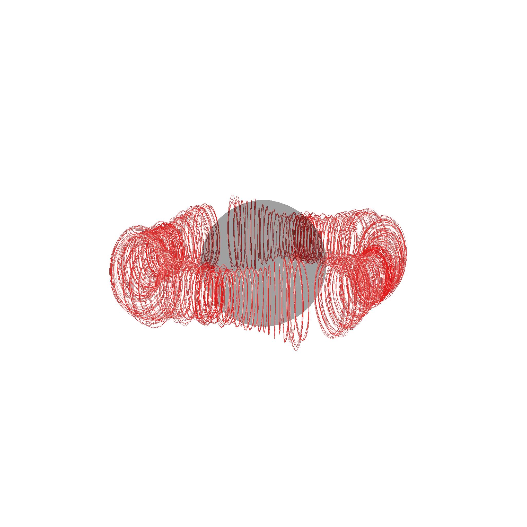
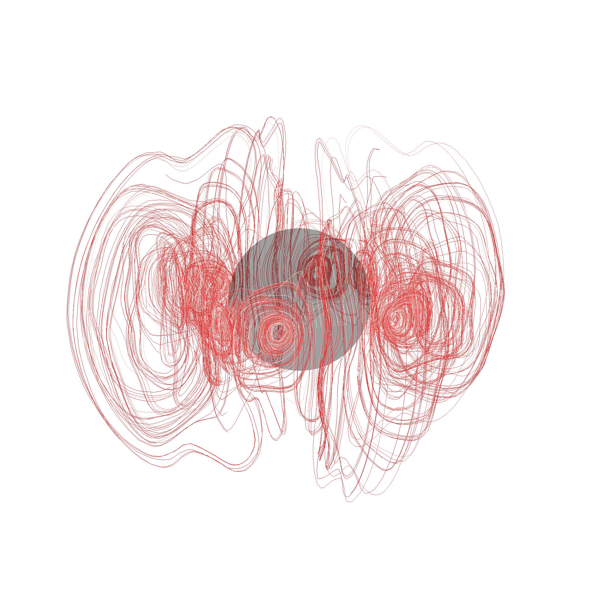
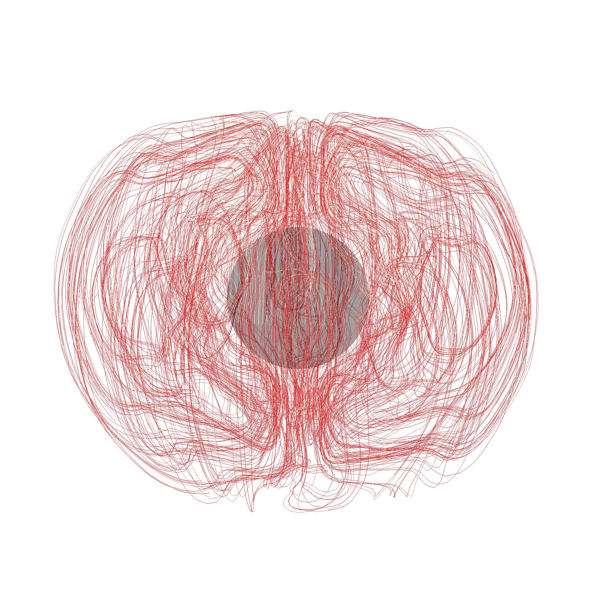
Figure 11: Evolution of magnetic streamlines seeded in equatorial plane at radius $5.91$ km. Gray isocontour shows surface of $\rho=6.18\times 10^{14}{\rm g\,cm^{-3}}$. Left: Varicose instability at $t=4.93$ ms. Middle: Kink instability at $t=12.8$ ms. Right: Late time non-linear field arrangement $t=44.3$ ms. (Figure adapted from Cook:2023bag ).

0.4.2 Gravitational collapse of Rotating Neutron Star

The ability of GR-Athena++ to handle gravitational collapse is confirmed, by simulating the unstable, uniformly rotating, equilibrium model D4 of Baiotti:2004wn ; Reisswig:2012nc ; Dietrich:2014wja . This model is triggered to collapse by the introduction of a perturbation to the pressure field of 0.5$\%$, following Dietrich:2014wja . The initial data is calculated with the RNS code of Stergioulas:1994ea with a central density of $\rho_{c}=1.924388\times 10^{15}{\rm g\,cm^{-3}}$ and a polar-to-equatorial coordinate axis ratio of $r_{p}/r_{e}=0.65$. This leads to a star with rotational frequency of $1276$ Hz, baryon mass of $M_{b}=2.0443{\rm M_{\odot}}$ and gravitational mass $M=1.8604{\rm M_{\odot}}$.

Our grid consists of 8 refinement levels, 3 of which lie within the star radius, with the outer boundaries the same as for §0.4.1, without imposed grid symmetries. We perform simulations with a base level resolution $N_{M}=32,64,128$ corresponding to finest grid spacings of $92.2,46.1,23.1$ m respectively, using PPM reconstruction. The evolution successfully passes through gravitational collapse and horizon formation without the need for excision.

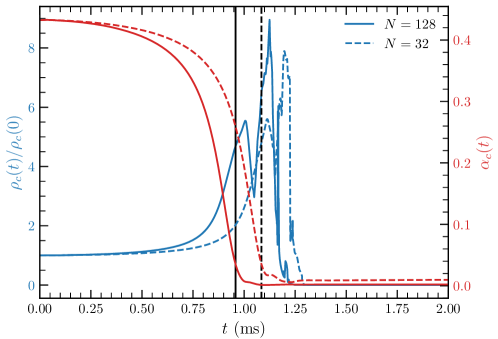
Figure 12: Collapsing D4 model for simulations wth PPM reconstruction. Evolution of central rest-mass density and lapse of at different resolutions. Vertical black lines denote collapse time for each simulation. Oscillatory behaviour occurs within the horizon, after collapse. (Figure adapted from Cook:2023bag ).

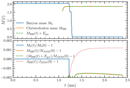
Figure 13: Collapsing D4 model for simulations wth PPM reconstruction. Top: Evolution of baryon mass and black hole (Christodoulou) mass for $N_{M}=32$. The dashed line shows the sum of the black hole mass and the gravitational-wave energy in the $(2,0)$ mode extracted at the coordinate sphere. Bottom: Baryon mass and angular momentum conservation and relative differences of Christodoulou mass with and without gravitational-wave energy added with respect to the initial ADM mass. (Figure adapted from Cook:2023bag ).

We first monitor the central density and lapse as indicators of the star collapse (Fig. 12). As the density and hence curvature increase at the centre of the star, the moving puncture gauge conditions used here Thierfelder:2010dv , cause the lapse to collapse at the origin, and handle black hole formation.

Using an apparent horizon finder, employing the spectral fast-flow algorithm of Gundlach:1997us ; Alcubierre:1998rq we locate an apparent horizon (AH) after one ms, at which point we see losses of baryon mass from the grid (Fig. 13) as the determinant of the spatial metric becomes very large at the centre of collapse. Prior to this we see mass conservation with relative error $10^{-13}$ despite the presence of refinement boundaries within the star, providing a robust test of the flux correction of Athena++. From the AH shape we calculate the Christodoulou mass Christodoulou:1970wf of $M_{\rm BH}=1.857{\rm M_{\odot}}$ and angular momentum $J_{\rm BH}=1.884{\rm M_{\odot}}^{2}$G/c of the horizon. These values differ from the expected ADM mass and angular momentum of the space-time by a relative error of order $10^{-3}$ for the lowest resolution simulation $N_{M}=32$, when the energy loss through GWs is included, which improves as a function of resolution. These results favourably compare to previous tests for this model in Reisswig:2012nc ; Dietrich:2014wja .

Gravitational waveforms (§0.3.5) are extracted using geodesic spheres at radius $R=221$ km, and the dominant $(\ell,m)=(2,0)$ of the strain is computed integrating in time and adjusting for drift Baiotti:2008nf . In Fig 14 we demonstrate these as a function of the retarded time to the extraction spheres, given by $t-r_{*}$ with $r_{*}=r+2M\log(r/2M-1)$, and $r(R)$ the areal radius of the spheres of coordinate radius $R$ (the isotropic Schwarzschild radius).

The waveform can be characterised by an initial burst of unphysical radiation after which we see the “precursor-burst-ringdown” behaviour expected for gravitational collapse. At $t-r_{*}\simeq 1$ ms for run $N_{M}=128$ we see a local maximum in GW amplitude, corresponding to the formation of the AH, followed shortly after by the global maximum amplitude after collapse, with the quasi-normal mode oscillations of a perturbed Kerr BH forming the final part of the wave signal.

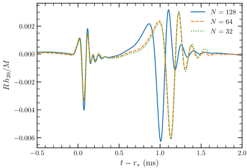
Figure 14: Dominant $(2,0)$ multipole of the gravitational strain for the collapsing D4 model for simulations wth PPM reconstruction. At $N_{M}=32$ the resolution is too low to observe convergent behaviour, though at higher resolutions we do see convergence in the waveforms at approximate first order. Note usage of geometric units on the vertical axis. (Figure adapted from Cook:2023bag ).

0.4.3 Binary Neutron Star space-times

The evolution of BNS space-times, and the extraction of highly accurate gravitational waveforms is a key target for GR-Athena++. We demonstrate this capability through direct, cross-code comparison of BNS evolution, without magnetic fields (GRHD), against the BAM code Bruegmann:1996kz ; Brugmann:2008zz ; Thierfelder:2011yi . Self consistency of GR-Athena++ is established through self-convergence of gravitational waveforms, together with good mass conservation for both GRHD and GRMHD simulations.

The initial data evolved is irrotational and constraint satisfying, as generated by the Lorene library Gourgoulhon:2000nn , describing a quasi-circular equal-mass merger with baryon mass $M_{b}=3.2500{\rm M_{\odot}}$ and gravitational mass $M=3.0297{\rm M_{\odot}}$ at an initial separation of $45$ km. The ADM mass of the binary is $M_{\rm ADM}=2.9984{\rm M_{\odot}}$, the angular momentum $J_{\rm ADM}=8.83542{\rm M_{\odot}}^{2}$G/c, and the initial orbital frequency is $f_{0}\simeq 294$ Hz.

An ideal gas EOS is used with $K=124$ and, in the case in which magnetic fields are present they are initialised as in the single star case with the vector potential in Eq. (27b), with $A_{b}$ chosen to give a maximum value of $1.77\times 10^{15}G$.

For runs with magnetic fields the grid outer boundaries are set at $[\pm 2268$, $\pm 2268$, $\pm 2268]$ km with no symmetry imposed. A refined static Mesh is defined with 7 levels of refinement, with the innermost grid covering both stars, from $[\pm 37,\pm 37,\pm 37]$ km. For runs without magnetic fields the grid is identical except for the imposition of bitant symmetry across the plane $z=0$. The Mesh parameters are $N_{M}=64,96,128$, corresponding to a grid spacing on the finest refinement level of $(554,369,277)$ m respectively. Simulations are performed with WENOZ reconstruction, and hydrodynamical variables are excised within the apparent horizon for runs with GRMHD.

Benchmark against BAM

From the beginning of the simulation with GRHD, the binary inspiral lasts for $\sim 3$ orbits before merging to form a massive remnant star that undergoes gravitational collapse at ${\sim}19$ ms for the lowest resolution simulation. In the case of GRMHD we see similar behaviour in the inspiral phase and visualise the the pre-merger, merger and pre-collapse phases in Fig. 15.

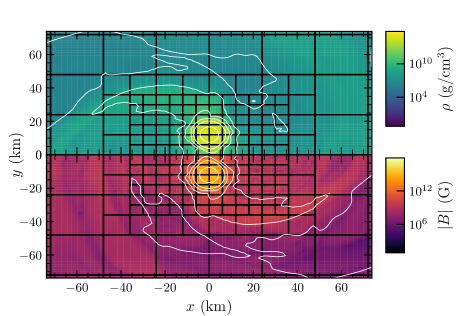
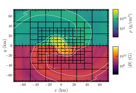
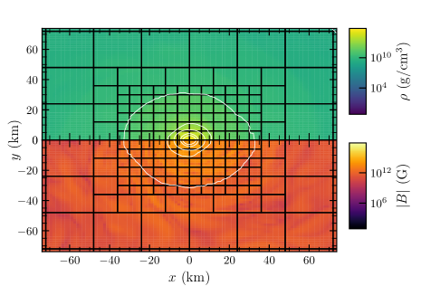
Figure 15: Snapshots of rest-mass density (upper half) and magnetic field strength (lower half) in the orbital plane. (Top, middle, bottom) correspond to respectively the final orbit ($t=5.96$ms), the moment of merger ($t=7.83$ms), and a late stage shortly before gravitational collapse $t=16$ms. White contours are lines of constant density at values $\rho=(6.18\times 10^{14},3.09\times 10^{14},6.18\times 10^{13},6.18\times 10^{12},6.18\times 10^{10},6.18\times 10^{8},6.18\times 10^{6},6.18\times 10^{4}){\rm g\,cm^{-3}}$. (Figure adapted from Cook:2023bag ).

We now directly compare to evolutions in BAM. GR-Athena++ and BAM employ slightly different hydrodynamical evolution schemes. For instance, the latter reconstructs the primitives using the fluid internal energy, rather than pressure as in GR-Athena++. BAM also lacks the intergrid operators of GR-Athena++ (§0.3.3), and uses a box-in-box style refinement strategy with Berger-Oliger time sub-cycling. For the sake of comparison, we perform two BAM simulations with differing hydrodynamical schemes, one using the LLF flux and WENOZ reconstruction similar to GR-Athena++, and one using the entropy flux-limited (EFL) scheme of Doulis:2022vkx , which is a fifth-order accurate scheme. The BAM grid uses six refinement levels, two of which move and contain the stars. The finest refinement level entirely covers the star at a resolution of ${\sim}461$ m, that is comparable to the GR-Athena++ grid configuration with $N_{M}=64$.

The conservation of baryon mass is depicted in Fig. 16 for the GRHD and GRMHD evolutions at different resolutions. The maximum violation of the relative conservation ${\sim}10^{-6}$ occurs at the lowest resolution. This error, while larger than for the single star, is sufficiently low to accurately study ejecta properties, and is consistent with other state-of-the-art Eulerian codes at the considered resolutions, e.g. Radice:2018pdn . It was found that through varying atmosphere parameter settings those leading to a mass increase provide the best mass conservation.

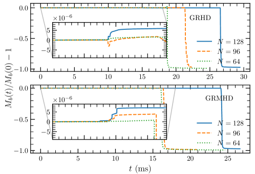
Figure 16: Baryon mass conservation for GRHD and GRMHD evolutions of the BNS. To the moment of merger, $t\simeq 7.5$ ms, the maximum relative violation is of the order $10^{-7}$. After merger, the violation increases to the $10^{-6}$ level. Note the mass typically increases due to atmosphere accretion. The abrupt drop of the mass at late times is due to black hole formation. (Figure adapted from Cook:2023bag ).

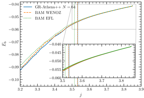
Figure 17: Binding energy vs angular momentum curves $E_{b}(j)$ for GR-Athena++ and BAM simulations. These quantities are computed following Damour:2011fu ; Bernuzzi:2012ci ; $E_{b}:=(M_{\mathrm{ADM}}-E_{\mathrm{GW}})\nu/(M-1)$, $j:=(J_{\mathrm{ADM}}-J_{\mathrm{GW}})/(M^{2}\nu)$, with $\nu$ the symmetric mass ratio, $\nu:=q/(1+q)^{2}$, $q>1$ the mass ratio and quantities suffixed with $\mathrm{GW}$ the contributions radiated away in gravitational waves. The moment of merger of each dataset is shown as vertical line. The inset captures energetics during the orbital phase, prior to the moment of merger. (Figure adapted from Cook:2023bag ).

To compare evolutions in a gauge invariant manner, curves of binding energy against angular momentum Damour:2011fu ; Bernuzzi:2012ci , are considered in Fig. 17. Close agreement up to merger at relatively low resolutions is found, with differences more pronounced post-merger. We note that the differences between GR-Athena++ and BAM are consistent with the internal differences between evolution schemes in BAM.

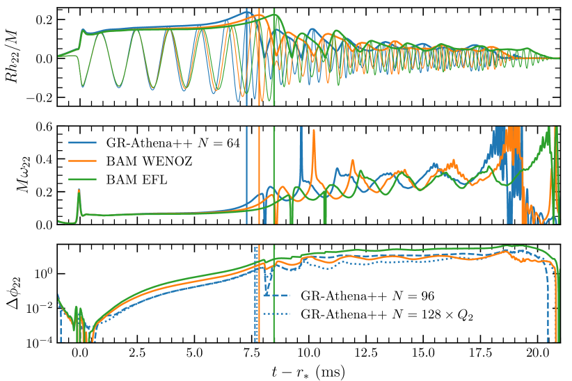
Figure 18: Waveform analysis and comparison with BAM. (Top): Real part and amplitude of strain mode $h{}_{22}$. We show: GR-Athena++ data with WENOZ reconstruction and $N_{M}=64$; BAM data with WENOZ reconstruction, and the EFL scheme at a similar resolution. (Middle): Instantaneous frequency of the waves for the three datasets. Note that in the top and middle panels the vertical axis is in geometric units. (Bottom): Phase differences between the GR-Athena++ data at $N_{M}=64$ and: $N_{M}=96$ (dashed); $N_{M}=128$ (dotted lines); and BAM data. GR-Athena++ phase difference data at $N_{M}=128$ is rescaled assuming $2^{\mathrm{nd}}{}$ convergence, matching with the $N_{M}=96$ data up to merger. The moment of merger of each dataset is indicated with a vertical line. (Figure adapted from Cook:2023bag ).

In Fig. 18, direct comparison of $h{}_{22}$ between the three runs is made. The top panel compares the real part of the gravitational wave strain, where we see amplitudes closely matching, and the main difference coming in the phasing. The earlier merger time of GR-Athena++ suggests that this run is slightly more dissipative than its BAM counterpart. Collapse time of runs is consistent to within $2.5$ ms.

The middle panel demonstrates the instantaneous gravitational wave frequency, which closely match at the moment of merger, $\omega_{22}\simeq 1340$ Hz for GR-Athena++ and BAM WENOZ and $\omega_{22}\simeq 1360$ Hz for BAM EFL. Similar consistency between runs is found in the frequency evolution of the post-merger remnant up to collapse, after which the quasi-normal modes of the remnant BH are insufficiently resolved, but are compatible with the fundamental mode frequency $\nu_{\rm QNM}\sim 6.5$ kHz ($M\omega_{22}\simeq 0.57$ in geometric units).

In the bottom panel of Fig. 18, phase differences of the GR-Athena++ $N_{M}=64$ run with respect to the BAM runs and the GR-Athena++ runs at higher resolutions are quantified. The difference between the $N_{M}=64$ and $N_{M}=128$ runs is rescaled by $Q_{2}$ to compare to the difference between the $N_{M}=64$ and $N_{M}=96$ run assuming $2^{\mathrm{nd}}{}$ order convergence. These curves closely match up to merger suggesting $2^{\mathrm{nd}}{}$ order convergence during the inspiral phase. Further, the difference to the BAM runs significantly reduces at higher resolutions.

Kelvin-Helmholtz instability

The Kelvin-Helmholtz instability (KHI) arises over a shearing interface in a fluid with a discontinuous velocity profile. This interface is unstable to perturbation, breaking down and forming small scale vortex like structures. It is suggested Price:2006fi that this should be expected during the merger of a BNS, as the two stars first make contact they shear past each other, creating an unstable interface. In the presence of magnetic fields numerical studies Kiuchi:2015sga ; Kiuchi:2017zzg ; Palenzuela:2021gdo ; Aguilera-Miret:2023qih support that KHI leads to magnetic field amplification.

As small scale vortices must be resolved, efficiency considerations motivate the use of targeted AMR. Here, two AMR criteria are demonstrated to capture $B$-amplification. We perform two SMR based simulations denoted SMR64 and SMR128, with the same grid configuration as those in §0.4.3 utilising Mesh sampling $N_{M}=64$ and $N_{M}=128$. The AMRB and AMR$\sigma$ runs are initialised from SMR64 after $t=4.93$ms, allowing an extra refinement level to be generated according to the appropriate criterion, bringing the maximum refinement up to that of run SMR128. Grid resolution is bounded below by that of SMR64.

In the case of AMRB, a MeshBlock (MB) is refined if its maximum value of $|B|$ exceeds $8.35\times 10^{13}$G and derefined if lower than this value. For AMR$\sigma$, a MB is refined if $\mathrm{max}_{\Omega_{i\in Z}}\sigma>4.50\times 10^{9}\mathrm{cm}/\mathrm{s}$, and derefined if $\mathrm{max}_{\Omega_{i\in Z}}\sigma<2.25\times 10^{9}\mathrm{cm}/\mathrm{s}$, where $\sigma:=\sqrt{((\Delta_{x}\tilde{u}^{y})^{2}+(\Delta_{y}\tilde{u}^{x})^{2})}$ represents the shear of the fluid velocity and $\Delta_{i}$ is the undivided difference operator in the $i$th direction.

The grid structure of run AMR$\sigma$ at $t=7.88\,\mathrm{ms}$, shortly before merger, is shown in Fig. 19, where small MBs generated at the star interface can be seen.

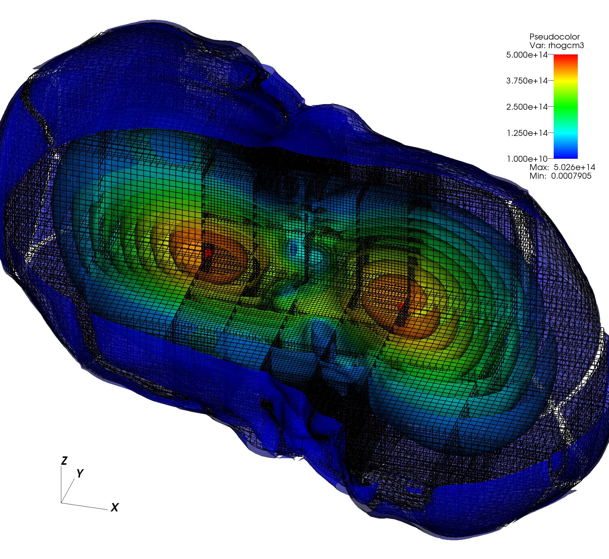
Figure 19: Mesh structure at $t=7.88$ms shortly before merger in the AMR$\sigma$ run. Isocontours of density are shown for $\rho>10^{11}{\rm g\,cm^{-3}}$. To reveal internal structure the $z>0,~{}y<0$ quadrant is suppressed. (Figure adapted from Cook:2023bag ).

The performance of an AMR criterion is judged on its ability to capture $B$-amplification, the $\#\mathrm{MB}$ generated (as a measure of efficiency), and the violation of the divergence free constraint of the magnetic field introduced through MB creation and destruction operations, demonstrated in the upper, middle and lower panels of Fig. 20 respectively.

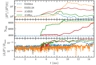
Figure 20: Top: Amplification of total magnetic field strength $|B^{2}|$ in BNS merger for SMR, AMRB, and AMR$\sigma$ refinement. Middle: Total $\#\mathrm{MB}$ present in each run. Bottom: $\partial_{i}B^{i}$ integrated over full computational domain $\Omega$ and normalised by $B_{\mathrm{max}}:=\max_{\Omega}B$. (Figure adapted from Cook:2023bag ).

In the upper panel we see that in SMR128 the energy is amplified by a factor of over 25 after the moment of merger, at $t\sim 10.2~{}$ms. The AMR simulations capture less of this amplification, with an AMRB amplification factor of 7.85, while AMR$\sigma$ only captures a factor of 3.26. In Kiuchi:2015sga , at considerably higher resolutions of $17.5$m a much larger amplification, of 6 orders of magnitude, from a much weaker initial magnetic field profile, of initial strength order $10^{13}$G is observed. Our expectation is that through addition of further levels of mesh refinement we should be able to capture such larger amplifications.

In the middle panel, we see that up to the moment of the peak magnetic field energy the run AMRB generates less than $10\%$ more MBs than SMR64, a factor of 1.79 fewer than SMR128 and a factor 1.91 fewer at the moment of merger. This supports the idea that targeted use of AMR can resolve magnetic field amplification. AMR$\sigma$ clearly however generates more MB than SMR128. This is due to MBs being generated at the star surface and in the region of unphysical ejecta from the merger. This criterion performs worse at capturing $B$-amplification, but shows improved mass conservation, which may have applications in ejecta tracking for simulations featuring physical ejecta.

Finally in the lower panel we see that the relative violation of the divergence-free constraint, as integrated over the domain, remains below $10^{-14}$ for the AMR runs. Note that, while the overall $\#\mathrm{MB}$ in the middle panel appears approximately constant, oscillations indicate continual destruction and creation of MeshBlock objects. Crucially, divergence preserving interpolation Toth:2002a , ensures an absence of any secular trends in $\partial_{i}B^{i}$ post AMR activation.

0.4.4 Scaling tests

The (binary, quad, oct)-tree based grid (§0.2.1), adaptive mesh refinement (§0.2.1), and parallel task-based execution featuring hybrid parallelism through MPI and OpenMP (§0.3.6) lead Athena++ to possess excellent scaling properties Stone:2020 . Here we confirm that, based on strong and weak scaling tests, extensions introduced in GR-Athena++ continue to preserve this. Our tests are performed in the context of evolution, with and without magnetic fields, of: BNS inspiral through to merger, and single NS (long term). Robust performance for demanding production grids, attained over multiple machines that involve a variety of architectures, is crucial for opening up the feasibility of very high resolution studies of these and related problems.

Scaling tests are performed on three clusters with different architectures: HLRS-HAWK; SUPERMUC-NG; and Frontera. The physical and grid configurations employed here match those described for the relevant problem in prior sections.

Strong scaling tests are performed by fixing the Mesh sampling $N_{M}$ of the unrefined grid and increasing the number of cores that the problem is solved on. For each choice of $N_{M}$ the physical extent of the innermost refined region is tuned to achieve a similar range of MeshBlock/core ratios across all series of resolutions.

The strong scaling efficiency is defined as $\eta_{S}:=1-\frac{t-t_{\mathrm{ideal}}}{t_{\mathrm{ideal}}}$ where $t$ is the elapsed wallclock time and $t_{\mathrm{ideal}}$ is the time expected for perfect strong scaling, halving exactly when resources are doubled.

Strong scaling tests are performed on HAWK and SuperMUC, where a given node is saturated with $32$ MPI tasks and $4$ OpenMP threads / task, and $12$ MPI tasks and $4$ OpenMP threads / task respectively.

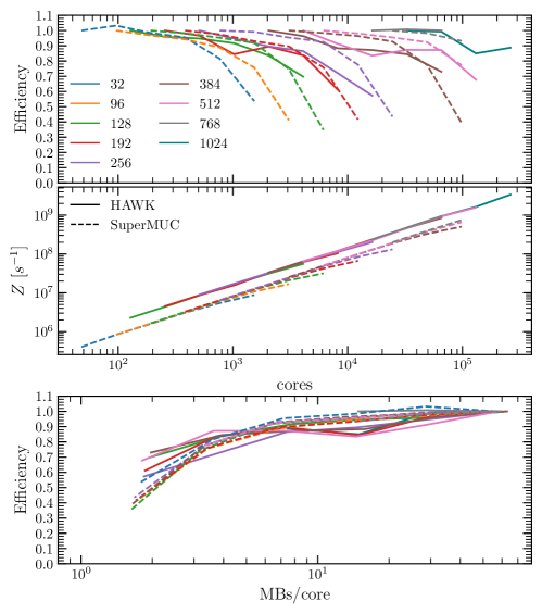
Figure 21: Strong scaling efficiency $\eta_{S}$ for the binary neutron star configuration with MHD. Results for HAWK and SuperMUC are included, up to $\mathcal{O}(10^{5})$ cores. Top: efficiency versus number of cores. Middle: zone cycles per second ($Z$) versus number of cores. Bottom: efficiency in terms of the MeshBlock to core ratio. (Figure adapted from Cook:2023bag ).

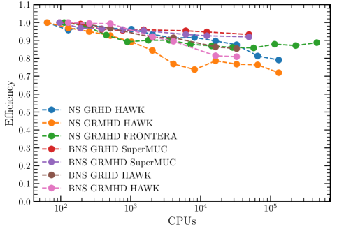
Figure 22: Weak scaling $\eta_{W}$ for SMR grids, over different target machines, for NS and BNS configurations with (GRMHD), and without (GRHD) magnetic fields. (Figure adapted from Cook:2023bag ).

In Fig. 21 we show the strong scaling performance for BNS with GRMHD. In the top panel, demonstrating efficiency against number of cores, we find efficiencies in excess of $80\%$ up to $\sim 10^{5}$ cores (gray and teal lines) for both SuperMUC (dashed lines) and HAWK (solid lines). An important aspect of maintaining high efficiencies is sufficiently saturating computational load Daszuta:2021ecf . This can be seen in Fig. 21 (lower) where the efficiency on SuperMUC is $\gtrsim 90\%$ as long as $\mathrm{\texttt{MeshBlock}{}/core}\gtrsim 6$, and the drop in efficiency on HAWK corresponding to this ratio dropping below $4$. The differences between machines are attributed to varied machine architectures. This causes a difference in the raw performance in terms of zone cycles per second ($Z$) (middle panel), where we observe runs on HAWK executing $\gtrsim 2$ faster than on SuperMUC. Comparable results found for simulations with magnetic fields disabled, and single NS configurations, have been omitted for brevity.

For weak scaling the executed zone cycles per second, $Z$, are measured. The expectation is that for perfect scaling, $Z$ should double every time the computational load and resources are concurrently doubled. The weak efficiency measure $\eta_{W}:=1-\frac{Z-Z_{\mathrm{ideal}}}{Z_{\mathrm{ideal}}}$ captures this.

In Fig 22 we demonstrate this weak scaling performance on the full range of machines and problems discussed above. Observe that scaling is maintained up to $\sim{}5\times 10^{5}$ CPU cores for the single star test at 89% efficiency on Frontera, with efficiencies dropping to, at worst 72% on HAWK. For binary tests we see an efficiency $\gtrsim 90\%$ up to $\sim{}5\times 10^{4}$ cores on SuperMUC-NG, with slightly lower efficiencies seen on HAWK for the same problem. This is also consistent with our previous vacuum sector tests Daszuta:2021ecf and those for stationary space-times Stone:2020 .

0.5 Summary and outlook

Our overview of GR-Athena++ for GRMHD simulations of astrophysical flows on dynamical space-times described several novel aspects we have introduced with respect to the original Athena++. In particular our treatment of: $\mathrm{Z}4$c coupling to GRMHD; equation of state; discretizations over differing grids including reconstruction; the constrained transport algorithm; conservative-to-primitive variable inversion; extraction of gravitational waves utilizing geodesic grids. When operation of these features is interwoven during GRMHD simulation, robust performance characteristics on multiple machines was demonstrated. Evolution on production grids in the absence of symmetries shows efficient use of exascale HPC architecture where: strong scaling efficiency in excess of $80\%$ up to $10^{5}$ CPU cores, and weak scaling efficiency of $89\%$ for $\sim{}5\times 10^{5}$ CPU cores is demonstrated.

Representative of the modeling challenges posed by astrophysical applications, benchmark problems were utilized to establish simulation quality of GR-Athena++ with focus on the absence of any simplifying symmetry reductions. This involved evolution of: isolated equilibrium NS over the long-term; unstable, rotating NS through gravitational collapse and black hole remnant; BNS inspiral through merger. Gravitational waveforms are shown to be convergent as resolution is increased, and consistent in cross-code comparison with BAM.

Anticipating full-scale simulations that seek to start tackling questions surrounding the open problems outlined in the introduction we presented novel simulations involving magnetic field instabilities. Long-term evolution of isolated magnetised NS with initially poloidal fields up to 68.7 ms extend our previous simulations Sur:2021awe to include a dynamical space-time. Similar results for the growth of a toroidal field component were found, saturating at approximately $10\%$ of the total magnetic field energy. In contrast, with the current GRMHD treatment of GR-Athena++, we find superior conservation of the internal energy of the NS, and total relative violations of the magnetic field divergence-free condition of the order of machine round-off. Similarly, we show that the KHI may be efficiently resolved through our AMR infrastructure. Indeed even initial low resolutions yield an amplification of a factor $\sim{}8$ with a single, additional level of refinement whilst utilizing approximately half the number of MeshBlock objects at the moment of merger when contrasted with a comparable static mesh refinement approach.

Active work on GR-Athena++ is underway so as to incorporate high-order schemes Radice:2013hxh ; Bernuzzi:2016pie ; Doulis:2022vkx essential for further improving waveform convergence and quality. The neutrino transport scheme developed by Radice:2021jtw is presently being ported together with an improved treatment of weak reactions and reaction rates. In future we also plan to couple the recently developed radiation solvers of Bhattacharyya:2022bzf ; White:2023wxh . Once these developments are mature, it is our intention to make GR-Athena++ publicly available.

- (1) Abbott, B. P., et al. Gravitational Waves and Gamma-Rays from a Binary Neutron Star Merger: GW170817 and GRB 170817A. Astrophys. J. 848, 2 (2017), L13, 1710.05834.
- (2) Abbott, B. P., et al. GW170817: Observation of Gravitational Waves from a Binary Neutron Star Inspiral. Phys. Rev. Lett. 119, 16 (2017), 161101, 1710.05832.
- (3) Abbott, B. P., et al. Multi-messenger Observations of a Binary Neutron Star Merger. Astrophys. J. 848, 2 (2017), L12, 1710.05833.
- (4) Aguilera-Miret, R., Palenzuela, C., Carrasco, F., and Viganò, D. The role of turbulence and winding in the development of large-scale, strong magnetic fields in long-lived remnants of binary neutron star mergers. 2307.04837.
- (5) Alcubierre, M., Brandt, S., Bruegmann, B., Gundlach, C., Masso, J., Seidel, E., and Walker, P. Test beds and applications for apparent horizon finders in numerical relativity. Class. Quant. Grav. 17 (2000), 2159–2190, gr-qc/9809004.
- (6) Alcubierre, M., Brügmann, B., Diener, P., Koppitz, M., Pollney, D., et al. Gauge conditions for long term numerical black hole evolutions without excision. Phys.Rev. D67 (2003), 084023, gr-qc/0206072.
- (7) Alic, D., Bona-Casas, C., Bona, C., Rezzolla, L., and Palenzuela, C. Conformal and covariant formulation of the Z4 system with constraint-violation damping. Phys.Rev. D85 (2012), 064040, 1106.2254.
- (8) Alic, D., Kastaun, W., and Rezzolla, L. Constraint damping of the conformal and covariant formulation of the Z4 system in simulations of binary neutron stars. Phys. Rev. D88, 6 (2013), 064049, 1307.7391.
- (9) Anderson, M., Hirschmann, E., Liebling, S. L., and Neilsen, D. Relativistic MHD with Adaptive Mesh Refinement. Class.Quant.Grav. 23 (2006), 6503–6524, gr-qc/0605102.
- (10) Arcavi, I., et al. Optical emission from a kilonova following a gravitational-wave-detected neutron-star merger. Nature 551 (2017), 64, 1710.05843.
- (11) Arnowitt, R. L., Deser, S., and Misner, C. W. Dynamical Structure and Definition of Energy in General Relativity. Phys. Rev. 116 (1959), 1322–1330.
- (12) Baiotti, L., Bernuzzi, S., Corvino, G., De Pietri, R., and Nagar, A. Gravitational-Wave Extraction from Neutron Stars Oscillations: comparing linear and nonlinear techniques. Phys. Rev. D79 (2009), 024002, 0808.4002.
- (13) Baiotti, L., Hawke, I., Montero, P. J., Loffler, F., Rezzolla, L., et al. Three-dimensional relativistic simulations of rotating neutron star collapse to a Kerr black hole. Phys.Rev. D71 (2005), 024035, gr-qc/0403029.
- (14) Baker, J. G., Centrella, J., Choi, D.-I., Koppitz, M., and van Meter, J. Gravitational wave extraction from an inspiraling configuration of merging black holes. Phys. Rev. Lett. 96 (2006), 111102, gr-qc/0511103.
- (15) Balbus, S. A., and Hawley, J. F. A Powerful Local Shear Instability in Weakly Magnetized Disks. I. Linear Analysis. Astrophys. J. 376 (July 1991), 214.
- (16) Banyuls, F., Font, J. A., Ibanez, J. M. A., Marti, J. M. A., and Miralles, J. A. Numerical 3+1 General Relativistic Hydrodynamics: A Local Characteristic Approach. Astrophys. J. 476 (1997), 221.
- (17) Baumgarte, T. W., and Shapiro, S. L. On the numerical integration of Einstein’s field equations. Phys. Rev. D59 (1999), 024007, gr-qc/9810065.
- (18) Beckwith, K., and Stone, J. M. A Second Order Godunov Method for Multidimensional Relativistic Magnetohydrodynamics. Astrophys. J. Suppl. 193 (2011), 6, 1101.3573.
- (19) Berger, M. J., and Colella, P. Local adaptive mesh refinement for shock hydrodynamics. Journal of Computational Physics 82 (May 1989), 64–84.
- (20) Berger, M. J., and Oliger, J. Adaptive Mesh Refinement for Hyperbolic Partial Differential Equations. J.Comput.Phys. 53 (1984), 484.
- (21) Bernuzzi, S., and Dietrich, T. Gravitational waveforms from binary neutron star mergers with high-order weighted-essentially-nonoscillatory schemes in numerical relativity. Phys. Rev. D94, 6 (2016), 064062, 1604.07999.
- (22) Bernuzzi, S., and Hilditch, D. Constraint violation in free evolution schemes: comparing BSSNOK with a conformal decomposition of Z4. Phys. Rev. D81 (2010), 084003, 0912.2920.
- (23) Bernuzzi, S., Nagar, A., Thierfelder, M., and Brügmann, B. Tidal effects in binary neutron star coalescence. Phys.Rev. D86 (2012), 044030, 1205.3403.
- (24) Bhattacharyya, M. K., and Radice, D. A Finite Element Method for Angular Discretization of the Radiation Transport Equation on Spherical Geodesic Grids. 2212.01409.
- (25) Blinnikov, S. I., Novikov, I. D., Perevodchikova, T. V., and Polnarev, A. G. Exploding Neutron Stars in Close Binaries. Soviet Astronomy Letters 10 (Apr. 1984), 177–179, 1808.05287.
- (26) Bona, C., Ledvinka, T., Palenzuela, C., and Zacek, M. General-covariant evolution formalism for Numerical Relativity. Phys. Rev. D67 (2003), 104005, gr-qc/0302083.
- (27) Bona, C., Massó, J., Seidel, E., and Stela, J. New Formalism for Numerical Relativity. Phys. Rev. Lett. 75 (1995), 600–603, gr-qc/9412071.
- (28) Borges, R., Carmona, M., Costa, B., and Don, W. S. An improved weighted essentially non-oscillatory scheme for hyperbolic conservation laws. Journal of Computational Physics 227, 6 (2008), 3191–3211.
- (29) Braithwaite, J., and Spruit, H. C. Evolution of the magnetic field in magnetars. Astron. Astrophys. 450 (2006), 1097, astro-ph/0510287.
- (30) Brandt, S., and Brügmann, B. A Simple construction of initial data for multiple black holes. Phys. Rev. Lett. 78 (1997), 3606–3609, gr-qc/9703066.
- (31) Brügmann, B. Adaptive mesh and geodesically sliced Schwarzschild spacetime in 3+1 dimensions. Phys. Rev. D54 (1996), 7361–7372, gr-qc/9608050.
- (32) Brügmann, B., Gonzalez, J. A., Hannam, M., Husa, S., Sperhake, U., et al. Calibration of Moving Puncture Simulations. Phys.Rev. D77 (2008), 024027, gr-qc/0610128.
- (33) Burstedde, C., Holke, J., and Isaac, T. On the Number of Face-Connected Components of Morton-Type Space-Filling Curves. Foundations of Computational Mathematics 19, 4 (Aug. 2019), 843–868.
- (34) Campanelli, M., Lousto, C. O., Marronetti, P., and Zlochower, Y. Accurate Evolutions of Orbiting Black-Hole Binaries Without Excision. Phys. Rev. Lett. 96 (2006), 111101, gr-qc/0511048.
- (35) Cao, Z., and Hilditch, D. Numerical stability of the Z4c formulation of general relativity. Phys.Rev. D85 (2012), 124032, 1111.2177.
- (36) Cheong, P. C.-K., Lam, A. T.-L., Ng, H. H.-Y., and Li, T. G. F. Gmunu: paralleled, grid-adaptive, general-relativistic magnetohydrodynamics in curvilinear geometries in dynamical space–times. Mon. Not. Roy. Astron. Soc. 508, 2 (2021), 2279–2301, 2012.07322.
- (37) Christodoulou, D. Reversible and irreversible transforations in black hole physics. Phys. Rev. Lett. 25 (1970), 1596–1597.
- (38) Ciolfi, R. Short gamma-ray burst central engines. Int. J. Mod. Phys. D 27, 13 (2018), 1842004, 1804.03684.
- (39) Ciolfi, R., Lander, S. K., Manca, G. M., and Rezzolla, L. Instability-driven evolution of poloidal magnetic fields in relativistic stars. Astrophys.J. 736 (2011), L6, 1105.3971.
- (40) Ciolfi, R., and Rezzolla, L. Twisted-torus configurations with large toroidal magnetic fields in relativistic stars. Mon. Not. Roy. Astron. Soc. 435 (2013), L43–L47, 1306.2803.
- (41) Cipolletta, F., Kalinani, J. V., Giacomazzo, B., and Ciolfi, R. Spritz: a new fully general-relativistic magnetohydrodynamic code. Class. Quant. Grav. 37, 13 (2020), 135010, 1912.04794.
- (42) Colella, P., Dorr, M. R., Hittinger, J. A. F., and Martin, D. F. High-order, finite-volume methods in mapped coordinates. Journal of Computational Physics 230, 8 (Apr. 2011), 2952–2976.
- (43) Combi, L., and Siegel, D. M. GRMHD Simulations of Neutron-star Mergers with Weak Interactions: r-process Nucleosynthesis and Electromagnetic Signatures of Dynamical Ejecta. Astrophys. J. 944, 1 (2023), 28, 2206.03618.
- (44) Combi, L., and Siegel, D. M. Jets from Neutron-Star Merger Remnants and Massive Blue Kilonovae. Phys. Rev. Lett. 131, 23 (2023), 231402, 2303.12284.
- (45) Cook, W., Daszuta, B., Fields, J., Hammond, P., Albanesi, S., Zappa, F., Bernuzzi, S., and Radice, D. GR-Athena++: General-relativistic magnetohydrodynamics simulations of neutron star spacetimes. 2311.04989.
- (46) Coulter, D. A., et al. Swope Supernova Survey 2017a (SSS17a), the Optical Counterpart to a Gravitational Wave Source. Science (2017), 1710.05452. [Science358,1556(2017)].
- (47) Curtis, S., Mösta, P., Wu, Z., Radice, D., Roberts, L., Ricigliano, G., and Perego, A. r-process nucleosynthesis and kilonovae from hypermassive neutron star post-merger remnants. Mon. Not. Roy. Astron. Soc. 518, 4 (2022), 5313–5322, 2112.00772.
- (48) Damour, T., Nagar, A., Pollney, D., and Reisswig, C. Energy versus Angular Momentum in Black Hole Binaries. Phys.Rev.Lett. 108 (2012), 131101, 1110.2938.
- (49) Daszuta, B., Zappa, F., Cook, W., Radice, D., Bernuzzi, S., and Morozova, V. GR-Athena++: Puncture Evolutions on Vertex-centered Oct-tree Adaptive Mesh Refinement. Astrophys. J. Supp. 257, 2 (2021), 25, 2101.08289.
- (50) de Haas, S., Bosch, P., Mösta, P., Curtis, S., and Schut, N. Magnetic field effects on nucleosynthesis and kilonovae from neutron star merger remnants. 2208.05330.
- (51) Dedner, A., Kemm, F., Kröner, D., Munz, C.-D., Schnitzer, T., and Wesenberg, M. Hyperbolic Divergence Cleaning for the MHD Equations. Journal of Computational Physics 175 (Jan. 2002), 645–673.
- (52) Dietrich, T., and Bernuzzi, S. Simulations of rotating neutron star collapse with the puncture gauge: end state and gravitational waveforms. Phys.Rev. D91, 4 (2015), 044039, 1412.5499.
- (53) Dimmelmeier, H., Stergioulas, N., and Font, J. A. Non-linear axisymmetric pulsations of rotating relativistic stars in the conformal flatness approximation. Mon. Not. Roy. Astron. Soc. 368 (2006), 1609–1630, astro-ph/0511394.
- (54) Doulis, G., Atteneder, F., Bernuzzi, S., and Brügmann, B. Entropy-limited higher-order central scheme for neutron star merger simulations. Phys. Rev. D 106, 2 (2022), 024001, 2202.08839.
- (55) Duez, M. D., Foucart, F., Kidder, L. E., Pfeiffer, H. P., Scheel, M. A., and Teukolsky, S. A. Evolving black hole-neutron star binaries in general relativity using pseudospectral and finite difference methods. Phys. Rev. D78 (2008), 104015, 0809.0002.
- (56) Duez, M. D., Liu, Y. T., Shapiro, S. L., and Stephens, B. C. Relativistic Magnetohydrodynamics In Dynamical Spacetimes: Numerical Methods And Tests. Phys. Rev. D72 (2005), 024028, astro-ph/0503420.
- (57) East, W. E., Pretorius, F., and Stephens, B. C. Hydrodynamics in full general relativity with conservative AMR. Phys.Rev. D85 (2012), 124010, 1112.3094.
- (58) Eichler, D., Livio, M., Piran, T., and Schramm, D. N. Nucleosynthesis, Neutrino Bursts and Gamma-Rays from Coalescing Neutron Stars. Nature 340 (1989), 126–128.
- (59) Etienne, Z. B., Paschalidis, V., Haas, R., Mösta, P., and Shapiro, S. L. IllinoisGRMHD: An Open-Source, User-Friendly GRMHD Code for Dynamical Spacetimes. Class. Quant. Grav. 32 (2015), 175009, 1501.07276.
- (60) Etienne, Z. B., Paschalidis, V., Liu, Y. T., and Shapiro, S. L. Relativistic MHD in dynamical spacetimes: Improved EM gauge condition for AMR grids. Phys.Rev. D85 (2012), 024013, 1110.4633.
- (61) Evans, C. R., and Hawley, J. F. Simulation of magnetohydrodynamic flows - A constrained transport method. Astrophys. J. 332 (Sept. 1988), 659–677.
- (62) Felker, K. G., and Stone, J. M. A fourth-order accurate finite volume method for ideal MHD via upwind constrained transport. Journal of Computational Physics 375 (Dec. 2018), 1365–1400.
- (63) Flowers, E., and Ruderman, M. A. Evolution of pulsar magnetic fields. Astrophys. J. 215 (July 1977), 302–310.
- (64) Font, J. A. Numerical hydrodynamics and magnetohydrodynamics in general relativity. Living Rev. Rel. 11 (2007), 7.
- (65) Font, J. A., et al. Three-dimensional general relativistic hydrodynamics. II: Long-term dynamics of single relativistic stars. Phys. Rev. D65 (2002), 084024, gr-qc/0110047.
- (66) Foucart, F., Duez, M. D., Kidder, L. E., and Teukolsky, S. A. Black hole-neutron star mergers: effects of the orientation of the black hole spin. Phys. Rev. D83 (2011), 024005, 1007.4203.
- (67) Gammie, C. F., McKinney, J. C., and Toth, G. HARM: A Numerical scheme for general relativistic magnetohydrodynamics. Astrophys.J. 589 (2003), 444–457, astro-ph/0301509.
- (68) Gardiner, T. A., and Stone, J. M. An unsplit Godunov method for ideal MHD via constrained transport. Journal of Computational Physics 205, 2 (May 2005), 509–539, astro-ph/0501557.
- (69) Gardiner, T. A., and Stone, J. M. An Unsplit Godunov Method for Ideal MHD via Constrained Transport in Three Dimensions. J. Comput. Phys. 227 (2008), 4123–4141, 0712.2634.
- (70) Giacomazzo, B., and Rezzolla, L. WhiskyMHD: a new numerical code for general relativistic magnetohydrodynamics. Class. Quant. Grav. 24 (2007), S235–S258, gr-qc/0701109.
- (71) Goldberg, J. N., MacFarlane, A. J., Newman, E. T., Rohrlich, F., and Sudarshan, E. C. G. Spin s spherical harmonics and edth. J. Math. Phys. 8 (1967), 2155.
- (72) Goldstein, A., et al. An Ordinary Short Gamma-Ray Burst with Extraordinary Implications: Fermi-GBM Detection of GRB 170817A. Astrophys. J. 848, 2 (2017), L14, 1710.05446.
- (73) Goodman, J. Are gamma-ray bursts optically thick? Astrophys. J. Lett. 308 (Sept. 1986), L47.
- (74) Gottlieb, S., Ketcheson, D. I., and Shu, C.-W. High Order Strong Stability Preserving Time Discretizations. Journal of Scientific Computing 38, 3 (Mar. 2009), 251–289.
- (75) Gourgoulhon, E., Grandclement, P., Taniguchi, K., Marck, J.-A., and Bonazzola, S. Quasiequilibrium sequences of synchronized and irrotational binary neutron stars in general relativity: 1. Method and tests. Phys.Rev. D63 (2001), 064029, gr-qc/0007028.
- (76) Gundlach, C. Pseudospectral apparent horizon finders: An Efficient new algorithm. Phys. Rev. D 57 (1998), 863–875, gr-qc/9707050.
- (77) Gundlach, C., Martin-Garcia, J. M., Calabrese, G., and Hinder, I. Constraint damping in the Z4 formulation and harmonic gauge. Class. Quant. Grav. 22 (2005), 3767–3774, gr-qc/0504114.
- (78) Hilditch, D., Bernuzzi, S., Thierfelder, M., Cao, Z., Tichy, W., and Bruegmann, B. Compact binary evolutions with the Z4c formulation. Phys. Rev. D88 (2013), 084057, 1212.2901.
- (79) Jiang, G.-S., and Shu, C.-W. Efficient Implementation of Weighted ENO Schemes. Journal of Computational Physics 126, 1 (June 1996), 202–228.
- (80) Kasen, D., Metzger, B., Barnes, J., Quataert, E., and Ramirez-Ruiz, E. Origin of the heavy elements in binary neutron-star mergers from a gravitational wave event. Nature (2017), 1710.05463. [Nature551,80(2017)].
- (81) Kastaun, W., Kalinani, J. V., and Ciolfi, R. Robust Recovery of Primitive Variables in Relativistic Ideal Magnetohydrodynamics. Phys. Rev. D 103, 2 (2021), 023018, 2005.01821.
- (82) Kidder, L. E., et al. SpECTRE: A Task-based Discontinuous Galerkin Code for Relativistic Astrophysics. J. Comput. Phys. 335 (2017), 84–114, 1609.00098.
- (83) Kiuchi, K., Cerdá-Durán, P., Kyutoku, K., Sekiguchi, Y., and Shibata, M. Efficient magnetic-field amplification due to the Kelvin-Helmholtz instability in binary neutron star mergers. Phys. Rev. D 92, 12 (2015), 124034, 1509.09205.
- (84) Kiuchi, K., Fujibayashi, S., Hayashi, K., Kyutoku, K., Sekiguchi, Y., and Shibata, M. Self-Consistent Picture of the Mass Ejection from a One Second Long Binary Neutron Star Merger Leaving a Short-Lived Remnant in a General-Relativistic Neutrino-Radiation Magnetohydrodynamic Simulation. Phys. Rev. Lett. 131, 1 (2023), 011401, 2211.07637.
- (85) Kiuchi, K., Held, L. E., Sekiguchi, Y., and Shibata, M. Implementation of advanced Riemann solvers in a neutrino-radiation magnetohydrodynamics code in numerical relativity and its application to a binary neutron star merger. Phys. Rev. D 106, 12 (2022), 124041, 2205.04487.
- (86) Kiuchi, K., Kyutoku, K., Sekiguchi, Y., and Shibata, M. Global simulations of strongly magnetized remnant massive neutron stars formed in binary neutron star mergers. Phys. Rev. D97, 12 (2018), 124039, 1710.01311.
- (87) Kiuchi, K., Kyutoku, K., Sekiguchi, Y., Shibata, M., and Wada, T. High resolution numerical-relativity simulations for the merger of binary magnetized neutron stars. Phys.Rev. D90, 4 (2014), 041502, 1407.2660.
- (88) Kiuchi, K., Shibata, M., and Yoshida, S. Evolution of neutron stars with toroidal magnetic fields: Axisymmetric simulation in full general relativity. Phys. Rev. D78 (2008), 024029, 0805.2712.
- (89) Kreiss, H. O., and Oliger, J. Methods for the approximate solution of time dependent problems. International Council of Scientific Unions, World Meteorological Organization, Geneva, 1973.
- (90) Kulkarni, S. R. Modeling supernova-like explosions associated with gamma-ray bursts with short durations. astro-ph/0510256.
- (91) Kumar, P., and Zhang, B. The physics of gamma-ray bursts \& relativistic jets. Phys. Rept. 561 (2014), 1–109, 1410.0679.
- (92) Lasky, P. D., Zink, B., Kokkotas, K. D., and Glampedakis, K. Hydromagnetic Instabilities in Neutron Stars. Astrophys. J. Lett. 735 (2011), L20, 1105.1895.
- (93) Li, L.-X., and Paczynski, B. Transient events from neutron star mergers. Astrophys.J. 507 (1998), L59, astro-ph/9807272.
- (94) Liebling, S. L., Lehner, L., Neilsen, D., and Palenzuela, C. Evolutions of Magnetized and Rotating Neutron Stars. Phys. Rev. D81 (2010), 124023, 1001.0575.
- (95) LIGO Scientific Collaboration. LIGO Algorithm Library - LALSuite. free software (GPL), 2018.
- (96) Liu, Y. T., Shapiro, S. L., Etienne, Z. B., and Taniguchi, K. General relativistic simulations of magnetized binary neutron star mergers. Phys. Rev. D78 (2008), 024012, 0803.4193.
- (97) Löffler, F., et al. The Einstein Toolkit: A Community Computational Infrastructure for Relativistic Astrophysics. Class. Quant. Grav. 29 (2012), 115001, 1111.3344.
- (98) Londrillo, P., and Del Zanna, L. On the divergence-free condition in godunov-type schemes for ideal magnetohydrodynamics: the upwind constrained transport method. J.Comput.Phys. 195 (2004), 17–48, astro-ph/0310183.
- (99) Markey, P., and Tayler, R. J. The adiabatic stability of stars containing magnetic fields. II. Poloidal fields. Mon. Not. R. Astron. Soc. 163 (Mar. 1973), 77–91.
- (100) Markey, P., and Tayler, R. J. The adiabatic stability of stars containing magnetic fields-III. Additional results for poloidal fields. Mon. Not. R. Astron. Soc. 168 (Sept. 1974), 505–514.
- (101) McCorquodale, P., Dorr, M. R., Hittinger, J. A. F., and Colella, P. High-order finite-volume methods for hyperbolic conservation laws on mapped multiblock grids. Journal of Computational Physics 288 (May 2015), 181–195.
- (102) Metzger, B., Martinez-Pinedo, G., Darbha, S., Quataert, E., Arcones, A., et al. Electromagnetic Counterparts of Compact Object Mergers Powered by the Radioactive Decay of R-process Nuclei. Mon.Not.Roy.Astron.Soc. 406 (2010), 2650, 1001.5029.
- (103) Morton, G. M. A computer oriented geodetic data base and a new technique in file sequencing. Tech. rep., 1966.
- (104) Mösta, P., Mundim, B. C., Faber, J. A., Haas, R., Noble, S. C., et al. GRHydro: A new open source general-relativistic magnetohydrodynamics code for the Einstein Toolkit. Class.Quant.Grav. 31 (2014), 015005, 1304.5544.
- (105) Mösta, P., Radice, D., Haas, R., Schnetter, E., and Bernuzzi, S. A magnetar engine for short GRBs and kilonovae. Astrophys. J. Lett. 901 (2020), L37, 2003.06043.
- (106) Narayan, R., Paczynski, B., and Piran, T. Gamma-ray bursts as the death throes of massive binary stars. Astrophys. J. 395 (1992), L83–L86, astro-ph/9204001.
- (107) Paczynski, B. Gamma-ray bursters at cosmological distances. Astrophys. J. 308 (1986), L43–L46.
- (108) Palenzuela, C., Aguilera-Miret, R., Carrasco, F., Ciolfi, R., Kalinani, J. V., Kastaun, W., Miñano, B., and Viganò, D. Turbulent magnetic field amplification in binary neutron star mergers. Phys. Rev. D 106, 2 (2022), 023013, 2112.08413.
- (109) Palenzuela, C., Miñano, B., Viganò, D., Arbona, A., Bona-Casas, C., Rigo, A., Bezares, M., Bona, C., and Massó, J. A Simflowny-based finite-difference code for high-performance computing in numerical relativity. Class. Quant. Grav. 35, 18 (2018), 185007, 1806.04182.
- (110) Pian, E., et al. Spectroscopic identification of r-process nucleosynthesis in a double neutron star merger. Nature (2017), 1710.05858.
- (111) Pili, A. G., Bucciantini, N., and Del Zanna, L. Axisymmetric equilibrium models for magnetized neutron stars in General Relativity under the Conformally Flat Condition. Mon. Not. Roy. Astron. Soc. 439 (2014), 3541–3563, 1401.4308.
- (112) Pili, A. G., Bucciantini, N., and Del Zanna, L. General relativistic models for rotating magnetized neutron stars in conformally flat space–time. Mon. Not. Roy. Astron. Soc. 470, 2 (2017), 2469–2493, 1705.03795.
- (113) Piran, T. The physics of gamma-ray bursts. Rev. Mod. Phys. 76 (2004), 1143–1210, astro-ph/0405503.
- (114) Plewa, T., and Mueller, E. The consistent multi-fluid advection method. Astron. Astrophys. 342 (1999), 179, astro-ph/9807241.
- (115) Pons, J. A., and Viganò, D. Magnetic, thermal and rotational evolution of isolated neutron stars. 1911.03095.
- (116) Pretorius, F. Evolution of binary black hole spacetimes. Phys. Rev. Lett. 95 (2005), 121101, gr-qc/0507014.
- (117) Price, D., and Rosswog, S. Producing ultra-strong magnetic fields in neutron star mergers. Science 312 (2006), 719, astro-ph/0603845.
- (118) Radice, D., Bernuzzi, S., Perego, A., and Haas, R. A new moment-based general-relativistic neutrino-radiation transport code: Methods and first applications to neutron star mergers. Mon. Not. Roy. Astron. Soc. 512, 1 (2022), 1499–1521, 2111.14858.
- (119) Radice, D., Perego, A., Hotokezaka, K., Fromm, S. A., Bernuzzi, S., and Roberts, L. F. Binary Neutron Star Mergers: Mass Ejection, Electromagnetic Counterparts and Nucleosynthesis. Astrophys. J. 869, 2 (2018), 130, 1809.11161.
- (120) Radice, D., Rezzolla, L., and Galeazzi, F. Beyond second-order convergence in simulations of binary neutron stars in full general-relativity. Mon.Not.Roy.Astron.Soc. 437 (2014), L46–L50, 1306.6052.
- (121) Radice, D., Rezzolla, L., and Galeazzi, F. High-Order Fully General-Relativistic Hydrodynamics: new Approaches and Tests. Class.Quant.Grav. 31 (2014), 075012, 1312.5004.
- (122) Randall, D. A., Ringler, T. D., Heikes, R., Jones, P., and Baumgardner, J. Climate modeling with spherical geodesic grids. Comput. Sci. Eng. 4 (2002), 32–41.
- (123) Rashti, A., Bhattacharyya, M., Radice, D., Daszuta, B., Cook, W., and Bernuzzi, S. Adaptive mesh refinement in binary black holes simulations, Dec. 2023, 2312.05438.
- (124) Rasio, F. A., and Shapiro, S. L. TOPICAL REVIEW: Coalescing binary neutron stars. Classical and Quantum Gravity 16, 6 (June 1999), R1–R29, gr-qc/9902019.
- (125) Reisswig, C., Haas, R., Ott, C. D., Abdikamalov, E., Mösta, P., Pollney, D., and Schnetter, E. Three-Dimensional General-Relativistic Hydrodynamic Simulations of Binary Neutron Star Coalescence and Stellar Collapse with Multipatch Grids. Phys. Rev. D87, 6 (2013), 064023, 1212.1191.
- (126) Ruiz, M., Hilditch, D., and Bernuzzi, S. Constraint preserving boundary conditions for the Z4c formulation of general relativity. Phys. Rev. D83 (2011), 024025, 1010.0523.
- (127) Ryu, D., Miniati, F., Jones, T. W., and Frank, A. A divergence-free upwind code for multidimensional magnetohydrodynamic flows. Astrophys. J. 509 (1998), 244, astro-ph/9807228.
- (128) Savchenko, V., et al. INTEGRAL Detection of the First Prompt Gamma-Ray Signal Coincident with the Gravitational-wave Event GW170817. Astrophys. J. 848, 2 (2017), L15, 1710.05449.
- (129) Shankar, S., Mösta, P., Brandt, S. R., Haas, R., Schnetter, E., and de Graaf, Y. GRaM-X: a new GPU-accelerated dynamical spacetime GRMHD code for Exascale computing with the Einstein Toolkit. Class. Quant. Grav. 40, 20 (2023), 205009, 2210.17509.
- (130) Shibata, M., and Nakamura, T. Evolution of three-dimensional gravitational waves: Harmonic slicing case. Phys. Rev. D52 (1995), 5428–5444.
- (131) Shibata, M., and Sekiguchi, Y.-i. Magnetohydrodynamics in full general relativity: Formulation and tests. Phys. Rev. D72 (2005), 044014, astro-ph/0507383.
- (132) Siegel, D. M., Ciolfi, R., and Rezzolla, L. Magnetically driven winds from differentially rotating neutron stars and X-ray afterglows of short gamma-ray bursts. Astrophys. J. 785 (2014), L6, 1401.4544.
- (133) Siegel, D. M., and Metzger, B. D. Three-Dimensional General-Relativistic Magnetohydrodynamic Simulations of Remnant Accretion Disks from Neutron Star Mergers: Outflows and -Process Nucleosynthesis. Phys. Rev. Lett. 119, 23 (2017), 231102, 1705.05473.
- (134) Siegel, D. M., Mösta, P., Desai, D., and Wu, S. Recovery schemes for primitive variables in general-relativistic magnetohydrodynamics. Astrophys. J. 859, 1 (2018), 71, 1712.07538.
- (135) Soares-Santos, M., et al. The Electromagnetic Counterpart of the Binary Neutron Star Merger LIGO/Virgo GW170817. I. Dark Energy Camera Discovery of the Optical Counterpart. Astrophys. J. 848, 2 (2017), L16, 1710.05459.
- (136) Stergioulas, N., and Friedman, J. L. Comparing models of rapidly rotating relativistic stars constructed by two numerical methods. Astrophys. J. 444 (1995), 306, astro-ph/9411032.
- (137) Stone, J. M., Gardiner, T. A., Teuben, P., Hawley, J. F., and Simon, J. B. Athena: A New Code for Astrophysical MHD. Astrophys. J. Suppl. 178 (2008), 137, 0804.0402.
- (138) Stone, J. M., Tomida, K., White, C. J., and Felker, K. G. The Athena++ Adaptive Mesh Refinement Framework: Design and Magnetohydrodynamic Solvers. Astrophys. J. Suppl. 249, 1 (July 2020), 4, 2005.06651.
- (139) Stout, Q. F., De Zeeuw, D. L., Gombosi, T. I., Groth, C. P. T., Marshall, H. G., and Powell, K. G. Adaptive blocks: A high performance data structure. In Proceedings of the 1997 ACM/IEEE Conference on Supercomputing (New York, NY, USA, Nov. 1997), SC ’97, Association for Computing Machinery, pp. 1–10.
- (140) Sur, A., Cook, W., Radice, D., Haskell, B., and Bernuzzi, S. Long-term general relativistic magnetohydrodynamics simulations of magnetic field in isolated neutron stars. Mon. Not. Roy. Astron. Soc. 511, 3 (2022), 3983–3993, 2108.11858.
- (141) Tayler, R. J. Hydromagnetic Instabilities of an Ideally Conducting Fluid. Proceedings of the Physical Society B 70, 1 (Jan. 1957), 31–48.
- (142) Tayler, R. J. The adiabatic stability of stars containing magnetic fields-I.Toroidal fields. Mon. Not. R. Astron. Soc. 161 (Jan. 1973), 365.
- (143) Thierfelder, M., Bernuzzi, S., and Brügmann, B. Numerical relativity simulations of binary neutron stars. Phys.Rev. D84 (2011), 044012, 1104.4751.
- (144) Thierfelder, M., Bernuzzi, S., Hilditch, D., Brügmann, B., and Rezzolla, L. The trumpet solution from spherical gravitational collapse with puncture gauges. Phys.Rev. D83 (2011), 064022, 1012.3703.
- (145) Tóth, G., and Roe, P. L. Divergence- and Curl-Preserving Prolongation and Restriction Formulas. Journal of Computational Physics 180, 2 (Aug. 2002), 736–750.
- (146) Typel, S., Oertel, M., and Klähn, T. CompOSE CompStar online supernova equations of state harmonising the concert of nuclear physics and astrophysics compose.obspm.fr. Phys. Part. Nucl. 46, 4 (2015), 633–664, 1307.5715.
- (147) Tóth, G. The constraint in shock-capturing magnetohydrodynamics codes. Journal of Computational Physics 161, 2 (2000), 605 – 652.
- (148) van Leer, B. Towards the Ultimate Conservation Difference Scheme. II. Monotonicity and Conservation Combined in a Second-Order Scheme. Journal of Computational Physics 14, 4 (Mar. 1974), 361–370.
- (149) Viganò, D., Martínez-Gómez, D., Pons, J. A., Palenzuela, C., Carrasco, F., Miñano, B., Arbona, A., Bona, C., and Massó, J. A Simflowny-based high-performance 3D code for the generalized induction equation. 1811.08198.
- (150) Wang, N., and Lee, J.-L. Geometric properties of the icosahedral-hexagonal grid on the two-sphere. SIAM Journal of Scientific Computing 33, 5 (2011), 2536–2559.
- (151) Weyhausen, A., Bernuzzi, S., and Hilditch, D. Constraint damping for the Z4c formulation of general relativity. Phys. Rev. D85 (2012), 024038, 1107.5539.
- (152) White, C. J., Mullen, P. D., Jiang, Y.-F., Davis, S. W., Stone, J. M., Morozova, V., and Zhang, L. An Extension of the Athena++ Code Framework for Radiation-magnetohydrodynamics in General Relativity Using a Finite-solid-angle Discretization. Astrophys. J. 949, 2 (2023), 103, 2302.04283.
- (153) White, C. J., Stone, J. M., and Gammie, C. F. An Extension of the Athena++ Code Framework for GRMHD Based on Advanced Riemann Solvers and Staggered-Mesh Constrained Transport. Astrophys. J. Suppl. 225, 2 (2016), 22, 1511.00943.
- (154) Wright, G. A. E. Pinch instabilities in magnetic stars. Mon. Not. R. Astron. Soc. 162 (Feb. 1973), 339–358.