An event generator for Lepton-Hadron Deep Inelastic Scattering at NLO+PS with POWHEG including mass effects

Abstract

We present a generator for lepton nucleon collisions in the DIS regime, focusing in particular on processes with a massive lepton and/or a massive quark in the final state. We have built a full code matching NLO QCD corrections to parton shower Monte Carlo programs in the POWHEG-BOX framework. Our code can be used to compute NLO+PS accurate fully differential predictions for neutral current and charged current processes, including processes with an incoming tau neutrino, and/or including charm quarks in the final state. We also made comparisons with available data and predictions for the new neutrino experiments at CERN.

1 Introduction

Lepton-hadron Deep Inelastic Scattering (DIS) has been a highly relevant framework for physics discoveries both for strong and weak interactions, most noticeably with the discovery of scaling at SLAC PhysRevD.5.528 , and with the discovery of weak neutral currents at CERN GargamelleNeutrino:1973jyy . Furthermore, DIS is the framework of choice for the measurement of parton density functions in the proton. Recently, two new experiments have begun taking data at the LHC, namely the FASER FASER:2023zcr and SND@LHC SNDLHC:2023pun , that exploit the large rate of forward neutrinos arising in $pp$ collisions, and promise access to tau neutrino interactions. The study of these neutrino interactions may have also applications regarding the air showers Reno:2023sdm .

The upcoming SHiP experiment SHiP:2015vad , a beam-dump experiment designed for the search of feebly interacting particles, will also study neutrino interactions. These, together with the plans for the Electron-Ion Collider (EIC) at BNL AbdulKhalek:2021gbh , and the consideration of future electron-hadron colliders in Europe, has generated a new interest in DIS processes also in the theory community.

The DIS cross section for unpolarised Charged Current (CC) neutrino or anti-neutrino scattering producing an outgoing charged lepton ${\ell^{\prime}}$ with mass $m_{{\ell^{\prime}}}$,

$$\nu/\bar{\nu}(l)+\leavevmode\nobreak\ N(P)\to{\ell^{\prime}}/\bar{{\ell^{\prime}}}({l^{\prime}})+\leavevmode\nobreak\ X(P_{X})\,,$$ (1)

is given by

$$\begin{split}\frac{\mathrm{d}^{2}\sigma^{CC}_{\nu/{\bar{\nu}}}}{\mathrm{d}x_{\rm bj}\mathrm{d}y}&=\frac{G^{2}_{F}ME_{\nu}}{\pi(1+Q^{2}/M^{2}_{W})}\biggl{\{}\biggl{(}y^{2}x_{\rm bj}+\frac{m^{2}_{\ell^{\prime}}y}{2E_{\nu}M}\biggr{)}F^{CC}_{1}(x_{\rm bj},Q^{2})\\ &+\biggl{[}\biggl{(}1-\frac{m^{2}_{\ell^{\prime}}}{4E^{2}_{\nu}}\biggr{)}-\biggl{(}1+\frac{Mx_{\rm bj}}{2E_{\nu}}\biggr{)}y\biggr{]}F^{CC}_{2}(x_{\rm bj},Q^{2})\\ &\pm\biggl{[}x_{\rm bj}y\biggl{(}1-\frac{y}{2}-\frac{m^{2}_{\ell^{\prime}}y}{4E_{\nu}M}\biggr{)}\biggr{]}F^{CC}_{3}(x_{\rm bj},Q^{2})\\ &+\frac{m^{2}_{\ell^{\prime}}(m^{2}_{\ell^{\prime}}+Q^{2})}{4E^{2}_{\nu}M^{2}x_{\rm bj}}F^{CC}_{4}(x_{\rm bj},Q^{2})-\frac{m^{2}_{\ell^{\prime}}}{E_{\nu}M}F^{CC}_{5}(x_{\rm bj},Q^{2})\biggr{\}},\end{split}$$ (2)

where $E_{\nu}$ is the energy of the incoming neutrino (or anti-neutrino) in the nucleon rest frame, $M_{W}$ and $G_{F}$ are the $W$ boson mass and the Fermi coupling constant, and $x_{\rm bj},y$ are the usual DIS parameters, defined as

$$\begin{split}Q^{2}&=-q^{2}=-(l-{l^{\prime}})^{2},\\ x_{\rm bj}&=\frac{Q^{2}}{2P\cdot q},\\ y&=\frac{P\cdot q}{P\cdot l},\\ M_{X}^{2}&=(l+P-{l^{\prime}})^{2}=P_{X}^{2}.\end{split}$$ (3)

The contribution of the $F_{4}$ and $F_{5}$ structure functions to the cross section in eq. (2) is suppressed for small lepton masses. This makes the tau leptons the only viable mean of accessing these two so far unmeasured structure functions via charged-current tau-neutrino DIS. Moreover, in the parton model the connection among $F_{4}$ and $F_{5}$ and the other structure functions is straightforward at lowest order, making their prediction very simple and solid. A measurement of these two structure functions would then provide further knowledge about the structure of the proton, and, beyond that, a further consistency test of the partonic picture through the verification of their relations with the other structure functions. Furthermore, a precise measurements of $F_{4}$ and $F_{5}$ might be useful to constraint those scenarios of Beyond Standard Model (BSM) physics at higher scales possibly related to the leptons of the third generation, that could alter the contribution of one or another of the form factors to the cross section in eq. (2) (see for example ref. Liu:2015rqa ).

Another relevant phenomenological domain is the production of massive charmed resonances in charged current DIS. This process can be used to further constraint the uncertainty on proton strangeness (see for example ref. Alekhin:2015byh ) that has an impact on $W$ boson mass extraction at hadron colliders. In fact, at 7 TeV, approximately 25% of the inclusive $W$ boson production rate is induced by at least one second-generation quark, $s$ or $c$, in the initial state ATLAS:2017rzl . This fraction increases with the center-of-mass energy.

The associated production of a tau lepton and a charm resonance in tau neutrino DIS might be measurable at SND@LHC and SHiP. The open production of a charm quark and tau lepton with an invariant mass larger than the typical mass of a bottom resonance could in principle probe new physics scenarios that cannot be explored at B factories.

The status of higher order calculations has reached a remarkable N³LO accuracy both for DIS structure functions Moch:2004xu ; Vermaseren:2005qc ; Moch:2008fj ; Davies:2016ruz ; Blumlein:2022gpp and for jet production in DIS Currie:2018fgr ; Gehrmann:2018odt , and at N²LO level for polarised DIS Borsa:2022cap . For the massive cases, NLO QCD corrections have been calculated since long Gottschalk:1980rv ; Gluck:1996ve ; Kretzer:2002fr . The massive structure functions have been first evaluated in the asymptotic limit Buza:1996wv ; Blumlein:2014fqa , and then at full NNLO level Berger:2016inr .

As far as fully exclusive Monte Carlo generators are concerned, while the current status of the calculations for collider processes is at the cutting-edge with the standard accuracy given by NLO+PS and also NNLO+PS for some classes of processes, the situation for DIS is less advanced. General-purpose Monte Carlo events generators, as HERWIG7 Bahr:2008pv ; Bellm:2019zci , SHERPA2 Gleisberg:2008ta ; Sherpa:2019gpd and PYTHIA8 Sjostrand:2014zea , widely used for hadron-hadron collisions can be also used to simulate massless DIS processes. For the massless case, a NLO+PS implementation is available within the HERWIG7 generator Carli:2010cg and, more recently, POWHEG based generators have been presented in ref. Banfi:2023mhz and ref. Borsa:2024rmh for the unpolarised and polarised DIS respectively. Furthermore, an NNLO+PS implementation in the UNNLOPS framework has appeared Hoche:2018gti , still for the massless case.

A widely used tool for full simulation of neutrino-nucleon interactions is the generator GENIE Andreopoulos:2009rq . For the case of DIS, it does not rely on standard procedures for matching fixed-order corrections with a parton shower. Instead, Born level events are generated according to the higher-order but inclusive result (i.e. according to the structure functions) and, then, subsequently processed with PYTHIA, as discussed in ref. Garcia:2020jwr . This procedure ensures that the outgoing lepton has the correct kinematics assuming that the parton shower adopts a recoil scheme which affects only the coloured partons.

In the present paper we aim to fill the gap, in particular for massive final states, and we present a full event generator to describe DIS events for both Neutral and Charged Current interactions (NC and CC respectively from now on). In order to do this we first consider the relevant QCD radiative corrections, then exploit the POWHEG method Nason:2004rx ; Frixione:2007vw ; Alioli:2010xd to match a Next-to-Leading (NLO) fixed order computation to a Shower Monte Carlo (SMC) program.

The paper is structured as follows. In section 2 we outline the basic aspects of our computation, referring to the appendix for the derivation of the relevant formulae and other technical details. We also show validation results for both the fixed order computations and showered event samples. In section 3 we present a selection of phenomenologically relevant results and perform comparisons with available data. We draw our conclusions in section 4.

2 Description of the calculation

Figure 1: Born, Virtual and Real emission sample diagrams for lepton-nucleon DIS, $\ell+N\rightarrow{\ell^{\prime}}+X$.

In this section we describe the main steps to develop a full event generator for the simulation of lepton-hadron DIS processes with NLO+PS accuracy. We start by considering fixed-energy incoming leptons.

The first step corresponds to implement a differential NLO calculation for the DIS processes. We have re-derived analytic expressions for all needed Born, Virtual and Real matrix elements for both NC and CC DIS interactions with massive or massless particles in the final state. Sample diagrams are shown in figure 1. We have double checked their numerical implementation with GoSam GoSam:2014iqq .

The second ingredient needed to perform the NLO computation is a subtraction scheme for the infrared and collinear divergences. The POWHEG-BOX framework implements the Frixione-Kunszt-Signer (FKS) Frixione:1995ms subtraction scheme that enforces a partition of the real emission phase space according to the collinear singularities of the real matrix elements. As is the case for any local subtraction scheme, we need to provide suitable momentum mappings connecting a Born phase space configuration plus a set of radiation variables to a real phase space configuration. There is some freedom in the choice of these mappings. While the particular map has no effect on pure NLO results, it has an impact when one matches the NLO computation to an SMC program. For the DIS case, a generic map may introduce some distortions in the distributions of the leptonic variables that are unnatural when only QCD corrections are considered.

To be more explicit, let us consider for example a CC DIS process with an initial state lepton scattering off a light quark in the proton producing a lepton and a massive quark. In the FKS scheme the real emission corrections to this process has only one initial-state collinear-singular configuration (for each real subprocess) and no final-state collinear singularities, thanks to the mass of the final-state quark that acts as a regulator of the collinear divergence.

We observe that, starting from a Born configuration and a set of radiation variables, the default initial-state mapping in the POWHEG-BOX is built so that it preserves the invariant mass and the rapidity of the Born final state partonic system. This choice is particularly suitable for hadron-hadron collisions with production of massive resonances. The prize is that both initial state momenta are not preserved. In our case this would imply a real event with a more energetic incoming lepton with respect to the starting Born configuration. This leads to an inconsistent formulation of the subtraction procedure for fixed-energy incoming leptons. Furthermore, at the time of event generation, the default POWHEG initial-state mapping would also change the momentum of the final state lepton, and this change will not be modified by the SMC program, which for the time being is supposed to not alter the momenta of the leptons. This second problem might alter the value of fiducial cross sections in passing from the NLO to NLO+PS results when, for example, a cut on $Q^{2}$ is applied. When available in the SMC program, one can choose different recoil schemes to assess the corresponding matching uncertainties, but a construction that preserves the leptonic momenta seems more justified on a physical ground.

A first option to overcome, at least in part, the problems mentioned above consists in building a mapping for initial-state radiation (ISR) that preserves the energy of the initial lepton and the invariant mass of the Born system. A second and better solution is provided by a mapping preserving the momenta of both the initial- and final-state lepton. We remind that general formulae for such mappings in terms of invariants have been derived since long, see e.g. ref. Catani:1996vz . Nonetheless, their implementation within the FKS framework is more involved as one has to adopt the specific parametrisation of the radiation variables that is employed in the construction of the FKS counterterms obtained by means of the plus prescriptions.

Similar considerations also apply to final-state radiation (FSR) when one considers the production of a massless quark at Born level. In this case, the default mapping implemented in the POWHEG-BOX preserves the initial-state momenta, and so can be directly applied to the case of fixed-energy leptons. On the other hand, this mapping does not preserve the final-state lepton momentum as the radiation recoil is globally absorbed by all final-state particles.

For the massless case, ISR and FSR mappings preserving the leptonic momenta have been derived in ref. Banfi:2023mhz . We have derived their generalisation for a massive quark and lepton in the final state. We have verified that our formulae smoothly reduce to the ones in ref. Banfi:2023mhz when approaching the massless limit. Since the construction of these mappings is rather technical and the corresponding formulae quite lengthy, we report them in appendix A.

Before concluding this section, we make a comment on charm production in CC DIS. Beside the EW production mechanism considered in this work, which is sensitive to the strange content of the proton, charm (anti-)quarks can be produced also in final-state gluon splitting processes, as depicted in figure 2.

Figure 2: Sample diagram of charm-anti charm-pair production in gluon splitting.

The latter processes can be enhanced by the valence densities and can compete with the EW production. We observe that starting from NNLO, the distinction between the two production mechanisms becomes less clear. Nonetheless, working at NLO and in a scheme in which the charm is treated as a massive quark, as we do, the gluon splitting process is finite and can be treated separately. For the rest of the work we focus on the EW production mechanism only.

2.1 NLO validation

We have compared our POWHEG implementation of the NLO corrections to an explicit calculation of the inclusive double differential cross section formulae (see for example eq. (2) for the case of CC neutrino and anti-neutrino scattering). The relevant proton structure functions are obtained through the convolution of the parton densities with the NLO coefficient functions taken from Ref Furmanski:1981cw and ref. Kretzer:2002fr for the massless and massive case respectively.

Since for many cases and in many kinematic regions the corrections are rather small, for the purpose of validation, in Figure 3, 4 and 5 we show only the $\alpha_{s}$ contributions, i.e. for each distribution we plot the difference NLO – LO. To generate validation plots we have considered incoming leptons with fixed energy equal to 500 GeV in the nucleon rest frame and used the NNPDF31_nlo_as_0118_nf_4 PDFs NNPDF:2017mvq with $\alpha_{s}=0.118$ and $n_{f}=4$ through the LHAPDF interface Buckley:2014ana . For the renormalisation ($\mu_{\rm{R}}$) and factorisation ($\mu_{\rm{F}}$) scales we set $\mu^{2}_{\rm{R}}=\mu^{2}_{\rm{F}}=Q^{2}$. We also apply the kinematic cut $Q^{2}>4\,\rm{GeV}^{2}$ to stay in the DIS regime where perturbation theory is well applicable.

In particular, in Figure 3 we show the Björken $x_{\rm bj}$ and inelasticity ${y_{\rm dis}}$ distributions for $\nu_{e}$ and $\bar{\nu}_{e}$ CC DIS. The blue points are obtained with our implementation of DIS in the POWHEG-BOX while the red solid curve is the result of a direct numeric integration of DIS formulae given in terms of proton structure functions, as in eq. (2). This has been obtained using standard gaussian quadrature routines to perform the convolution of the parton densities with the coefficient functions.

In Figure 4 and 5, the same distributions are shown for the cases of $\nu_{e}$ (or $\bar{\nu}_{e}$) CC DIS producing a charm quark ($m_{c}=1.5\,$GeV), and $\nu_{\tau}$ (or $\bar{\nu}_{\tau}$) CC DIS producing a tau lepton ($m_{\tau}=1.777\,$GeV), respectively. For all initial and final state configurations, we found perfect agreement between the fixed-order results obtained with the POWHEG generator and the ones obtained with the direct calculation using the structure functions. We have also checked that the same level of agreement is achieved for all choices of the available momentum mappings employed in the subtraction procedure. This represents a non-trivial test of the newly derived DIS momentum mappings presented in appendix A. Additional sets of validation plots are reported in appendix B for completeness.

Figure 3: Order $\alpha_{s}$ contributions to Björken $x_{\rm bj}$ (left panels) and inelasticity ${y_{\rm dis}}$ (right panels) for CC $\nu_{e}$ (top panels) and $\bar{\nu}_{e}$ (bottom panels) DIS. We considered incoming $\nu_{e}$ ($\bar{\nu}_{e}$) with fixed energy equal to 500 GeV in the nucleon rest frame. We have used the NNPDF31_nlo_as_0118_nf_4 PDFs, set $\mu^{2}_{\rm{R}}=\mu^{2}_{\rm{F}}=Q^{2}$, and applied the kinematic cut $Q^{2}>4\,\rm{GeV}^{2}$. The blue points are obtained with our implementation of DIS in the POWHEG-BOX while the red solid curve is the result of the structure function calculation.

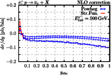
Figure 4: Same as figure 3 for charged current $\nu_{e}$ ($\bar{\nu}_{e}$) DIS with charm quark production setting $m_{c}=1.5\,$GeV.

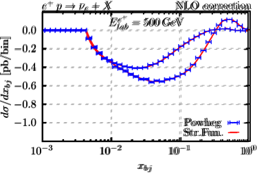
Figure 5: Same as figure 3 for charged current $\nu_{\tau}$ ($\bar{\nu}_{\tau}$) DIS with $m_{\tau}=1.777\,$GeV.

2.2 Event generation and impact of radiative corrections

The first emission is generated according to the POWHEG master formula Frixione:2007vw

$$d\sigma_{\textrm{NLO}}={\bar{B}}(\Phi_{B})d\Phi_{B}\left[\Delta_{\textrm{NLO}}(\Phi_{B},t_{\textrm{min}})+\sum_{\alpha}\frac{\left[d\Phi_{\textrm{rad}}\Delta_{\textrm{NLO}}(\Phi_{B},K_{T}(\Phi_{R}))R(\Phi_{R})\right]^{{\bar{\Phi}}_{B}^{\alpha}=\Phi_{B}}_{\alpha}}{B(\Phi_{B})}\right]\;,$$ (4)

where $\Phi_{B}$ is the Born phase space and $\Phi_{R}$ is the real phase space (that includes the radiation of one extra parton). $\Phi_{R}$ is mapped biunivocally into a Born and a radiation phase space, so that $\mathrm{d}\Phi_{R}=\mathrm{d}\Phi_{B}\,\mathrm{d}\Phi_{\rm rad}$. In the above equation, $B$ and $R$ are, respectively, the Born and real squared matrix elements averaged/summed over colors and spins, ${\bar{B}}$ entails the NLO corrections inclusively integrated over the radiation phase space. The sum runs over all the singular regions, labeled by $\alpha$, and the POWHEG Sudakov reads

$$\Delta_{\textrm{NLO}}(\Phi_{B},p_{T})=\Theta(p_{T}-t_{\textrm{min}})\exp\left\{-\sum_{\alpha}\int\frac{\left[d\Phi_{\textrm{rad}}R(\Phi_{R})\right]^{{\bar{\Phi}}_{B}^{\alpha}=\Phi_{B}}_{\alpha}}{B(\Phi_{B})}\Theta\left(K_{T}(\Phi_{R})-p_{T}\right)\right\}\;.$$ (5)

According to eq. (4), resolved radiation is generated with a hard scale, given by the $K_{T}$ function, down to some characteristic hadronic scale $t_{\textrm{min}}$, which in POWHEG is chosen to be $t_{\textrm{min}}=0.8\;\textrm{GeV}^{2}$.

The evolution variable $K_{T}(\Phi_{R})$ is a smooth function of the radiation variables, which is required to approach the transverse momentum of the radiated parton near the soft and collinear limits. For ISR, assuming that the incoming lepton is moving along the positive $z$-direction, we adopt the definition

$$K^{2}_{T}(\Phi_{R})\equiv K^{2}_{T}(\Phi_{B},\Phi_{\text{rad}})=\frac{{\bar{s}}}{2}\frac{\xi^{2}(1+y)}{1+\xi y}$$ (6)

where ${\bar{s}}$ is the CM energy of the underlying Born configuration $\Phi_{B}$, $\xi$ is twice the ratio of the radiated-parton energy over the partonic CM energy, and $y$ is the cosine of the angle of the radiated parton with respect to the positive $z$ axis in the partonic CM frame. Notice that the collinear limit, in this specific case, is given by $y\to-1$. The term $1+\xi y$ in the denominator, which reduces to $1$ in the soft limit, gives the correct behavior in the limit of a hard and collinear emission.

For FSR, we adopt the definition

$$K^{2}_{T}(\Phi_{R})\equiv K^{2}_{T}(\Phi_{B},\Phi_{\text{rad}})=\frac{{\bar{s}}}{2}\xi^{2}(1-y)$$ (7)

where, now, $y$ is the cosine of the angle between the radiation and the emitter parton. The interested reader can find further details on the generation of the radiation in appendix A.2.4 and appendix A.2.6 for ISR and FSR, respectively.

Since in POWHEG the decomposition in singular regions is driven by the collinear singularities, in the case of the production of a heavy quark there is only one FKS singular region, corresponding to ISR from the incoming light quark. On the other hand, the real matrix element may be enhanced when the extra gluon is emitted quasi-collinearly to the final-state heavy quark. In this case, the choice of an ISR hard scale $K_{T}$ is not correct, possibly leading to a mismodeling of this configurations. A more consistent treatment of the FSR quasi-collinear region would require its inclusion in the FKS decomposition, see e.g. ref. Buonocore:2017lry , and the construction of a suitable mapping for the case of a massive emitter. While different mappings do exist Barze:2012tt ; Buonocore:2017lry , they have been devised in the context of hadron-hadron collisions. Since there the radiation recoil is shared by all particles in the final state, the leptonic variables are not preserved in such mappings, which are then not ideal for DIS processes.

In this work, we follow a different strategy. Despite being potentially large, the contribution of the quasi-collinear configurations is finite thanks to the heavy quark mass. Therefore, it can be generated separately as a regular (i.e non-singular) real component. To this end, we introduce a smooth decomposition of the real squared amplitude

$$R=w_{\textrm{QFSR}}R+(1-w_{\textrm{QFSR}})R\equiv R_{\textrm{QFSR}}+R_{\textrm{sing}}\;.$$ (8)

The contribution $R_{\textrm{sing}}$ contains all soft and/or collinear singularities and is suppressed in the FSR quasi-collinear configurations, which is instead dominant in $R_{\textrm{QFSR}}$. Then, we replace $R\to R_{\textrm{sing}}$ in the POWHEG Sudakov and in the ${\bar{B}}$ function, while we generate remnant events according to the distribution

$$R_{\textrm{QFSR}}(\Phi_{R})d\Phi_{R}$$ (9)

with standard Monte Carlo methods. In order to construct the $w_{\textrm{QFSR}}$ function we introduce the distances of the radiated parton with respect to the initial-state light quark $d_{\textrm{ISR}}$ and to the final-state massive quark $d_{\textrm{QFSR}}$

$$d_{\textrm{ISR}}=\frac{p\cdot k}{p^{0}},\quad d_{\textrm{QFSR}}=\frac{v\cdot k}{v^{0}}+m_{v},$$ (10)

where $p,v$ and $k$ are, respectively, the momentum of the incoming light quark, of the outgoing heavy quark, with mass $m_{v}=\sqrt{v^{2}}$, and of the radiation, with all energies evaluated in the partonic CM frame. Then, we write

$$w_{\textrm{QFSR}}=\frac{d_{\textrm{ISR}}}{d_{\textrm{ISR}}+d_{\textrm{QFSR}}}.$$ (11)

Notice, in particular, that in the soft limit $d_{\textrm{QFSR}}\to m_{v}$ while $d_{\textrm{ISR}}\to 0$, so that $w_{\textrm{QFSR}}\to 0$, which ensures that all singularities are contained in $R_{\textrm{sing}}$. The above remnant mechanism represents our default choice for DIS processes characterised by a heavy quark in the final state. Furthermore, in order to avoid issues related to real configurations whose underlying Born gives a vanishing or very small contribution, we always turn on the Bornzerodamp mechanism Alioli:2010xd in our POWHEG generator.

The calculation for the heavy quark production processes is performed in the decoupling scheme with $n_{f}=3$ active flavors in the running of $\alpha_{S}$ and in the proton. We are dealing with EW processes that are quark-initiated at the lowest order. As a consequence, the strong coupling is not renormalised by NLO corrections and the gluon parton density starts to contribute only at NLO. Therefore, we can consistently adopt PDF sets and $\alpha_{S}$ running with $n_{f}=4$ without the need of introducing any correction terms related to the change of scheme, see e.g. Cacciari:1998it . This matches what is done for all other cases involving only light quarks, where we consider a $n_{f}=4$ proton with a massless charm component to complete the second-generation $SU(2)$ doublet.

We focus on the following representative processes

• $e^{-}+p\to\nu_{e}+X$(no masses);

• $e^{-}+p\to\nu_{e}+\bar{c}+X$ (production of a massive quark);

• $\nu_{\tau}+p\to\tau^{-}+X$ (production of a massive lepton),

• $\nu_{\tau}+p\to\tau^{-}+c+X$ (production of a massive quark and a massive lepton),

which include all combination of massive quark/lepton in the final state.

In all cases, we consider a reference setup with an incoming lepton with fixed energy $E_{\ell}=1\,$TeV scattering off a proton at rest in the laboratory frame. A cut on the minimum momentum transfer $Q^{2}>4\,\textrm{GeV}^{2}$ is applied. The $W$ boson mass is set to $m_{W}=80.419\,$GeV, the $\tau$ mass to $m_{\tau}=1.777\,$GeV, the charm mass to $m_{c}=1.5\,$GeV, the Fermi constant to $G_{F}=1.16639\times 10^{-5}\,\textrm{GeV}^{-2}$, and the cosine of the Cabibbo angle to $\cos{\theta_{C}}=0.97462$. We use the NNPDF3.1 NLO PDFs NNPDF:2017mvq with $\alpha_{S}=0.118$ and $n_{f}=4$ through the LHAPDF interface Buckley:2014ana . We adopt a dynamical scale $\mu_{0}=\sqrt{Q^{2}+m_{v}^{2}}$, where $m_{v}$ is the mass of the final-state quark. We will refer in the following to the $Q^{2}>4\,\textrm{GeV}^{2}$ cut as the definition of our fiducial region.

In table 1, we list the LO and NLO rates in our fiducial region for

process	$\sigma_{\textrm{LO}}$ [pb] ]	$\sigma_{\textrm{NLO}}$ [pb]	$\sigma_{\textrm{NLO}}/\sigma_{\textrm{LO}}-1$ [%]
$e^{-}+p\to\nu_{e}+X$	$3.7881(3)$	$3.6741(6)$	$-3.0\%$
$e^{-}+p\to\nu_{e}+c+X$	$0.069706(15)$	$0.1056(4)$	$+51.5\%$
$e^{-}+p\to\nu_{e}+c+X,\,m_{c}=0$	$0.0644(2)$	$0.1039(4)$	$+61\%$
$\nu_{\tau}+p\to\tau^{-}+X$	$4.1228(5)$	$3.9571(8)$	$-4.0\%$
$\nu_{\tau}+p\to\tau^{-}+c+X$	$0.64706(6)$	$0.6217(2)$	$-3.9\%$

Table 1: Inclusive LO and NLO fiducial rates for the four considered processes. The result for a massless charm is also reported for comparison.

producing the final-state lepton (inclusively over any hadronic final state) or for producing the final-state lepton and the charm. In all cases but charm electro-production in CC, we find that the NLO corrections are rather mild, decreasing the rates by a few percents. The smallness of the NLO corrections is in part a result of relatively large positive and negative contributions, possibly occurring among subprocesses in the same $SU(2)$ weak doublet (neglecting Cabibbo suppressed mixing effects), that cancel to a large extent in the fiducial rates. We anticipate, therefore, that their impact on more differential observables may be larger.

On the other hand, in the case of charm electro-production, NLO corrections increase the LO fiducial rate by $61\%$. It is worth explaining why. The related process of charm neutrino-production does not feature the same large positive NLO correction. This is a first indication that the origin of the different behavior is not related to the massive calculation. Indeed, we can perform the calculation even for a massless charm by tagging the charm in the final state. The result for charm electro-production for a massless charm is reported in table 1 for comparison. We found that the NLO correction has the same pattern as that for the massive charm. This confirms that this pattern is not associated with mass effects and that logarithms of the charm mass are not extremely large at the energy scales probed by the considered lepton-proton scattering process.

On the other hand, a large positive correction can be associated to real emission processes populating regions of phase space that were inaccessible or dynamically suppressed at a lower order. Specifically, if we neglect all masses for simplicity, in the collision $e^{-}\bar{s}\to\nu_{e}\bar{c}$, in the partonic CM, $e^{-}$ and $\bar{s}$ have opposite helicity and thus the same spin along the collision direction. In backward scattering also $\nu_{e}$ and $\bar{c}$ have the same spin, but opposite to the incoming ones, so that angular momentum conservation is violated by two units, leading to a $(1-y_{\rm dis})^{2}$ suppression of the cross section. Conversely in the collision $\nu_{e}s\to e^{-}c$ the two incoming particles have opposite spin, and no such suppression arises. Therefore, in the case of charm electro-production, real emission processes can lift the dynamical suppression in the backward scattering region, leading to a large positive correction to the fiducial rates.

We focus now on the kinematic distributions of the following observables:

• the inclusive DIS leptonic variables, $x_{\rm bj}$ and ${y_{\rm dis}}$;

• the transverse momenta of the leading light-flavor (charm-flavor) jet $j_{1}$ ($j^{c}_{1}$) for the light (heavy) quark case and of the second leading light-flavor jet $j_{2}$;

• the rapidity $y_{j_{1}}$($y^{c}_{j_{1}}$) of the leading light-flavor (charm-flavor) jet in the lab frame and the lepton-jet $\Delta R_{\ell j_{1}}=\sqrt{\Delta^{2}y_{\ell j_{1}}+\Delta^{2}\phi_{\ell j_{1}}}$ ($\Delta R_{\ell j^{c}_{1}})$ separation.

We define the jets using the anti-$k_{T}$ clustering algorithm Cacciari:2008gp as implemented in FastJet Cacciari:2011ma , with radius $R=1$ and using the $E$-scheme for the recombination. The jets are required to have a minimum transverse momentum of $0.1\,$GeV. At parton level, jets containing any charm quarks and/or anti-quarks are considered charm-flavor jets.

We consider two variants of the momentum mappings:

• “global”: the ISR mapping preserves the momentum of the incoming lepton and the invariant mass of the underlying Born system (simple mapping for DIS), the FSR mapping preserves both incoming partons momenta (standard FKS FSR mapping implemented in the POWHEG-BOX);

• “dis”: both ISR and FSR mappings preserve the momenta of the incoming and outgoing leptons.

In fixed order perturbation theory, the two options must provide equivalent results. Differences may appear at the level of the events generated according to the POWHEG formula.

The kinematic distributions are reported in figures 6-9. In all plots, we compare predictions obtained

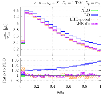
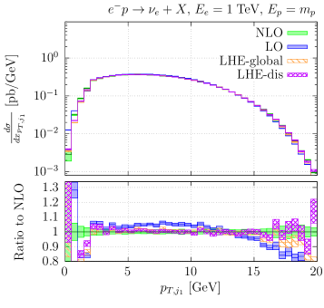
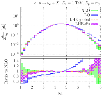
Figure 6: Collection of differential distributions for the scattering of a $1\,\textrm{TeV}$ electron off a proton at rest: Björken variable $x_{\rm bj}$, inelasticity ${y_{\rm dis}}$, transverse momentum of the leading jet $p_{T,j_{1}}$, transverse momentum of the second jet $p_{T,j_{2}}$, rapidity of the leading jet $y_{j_{1}}$, lepton-jet separation $\Delta R_{j_{1},{\ell^{\prime}}}$. LO predictions are displayed in blue, NLO ones in green, results obtained at the POWHEG event level in orange and in purple adopting, respectively, the “global” (LHE-global) and the “dis” (LHE-dis) settings. Ratios to NLO predictions are given in the bottom panels.

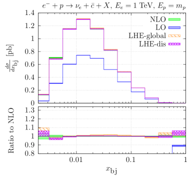
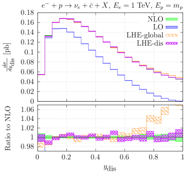
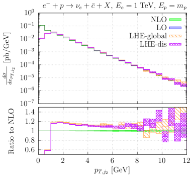
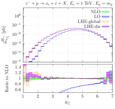
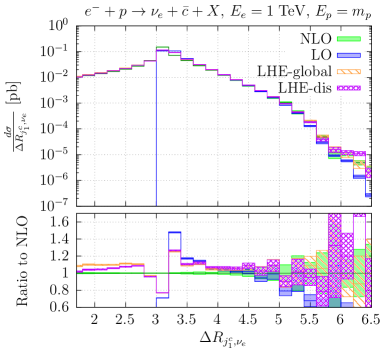
Figure 7: As in Fig 6 for the process $e^{-}+p\to\nu_{e}+\bar{c}+X$. The leading jet $j_{1}^{c}$ is the leading charm-flavor jet.

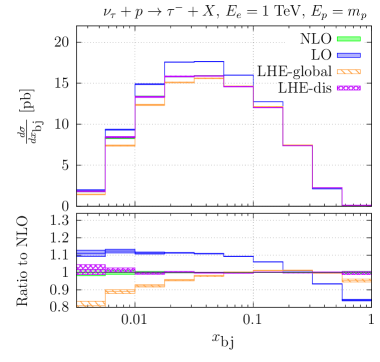
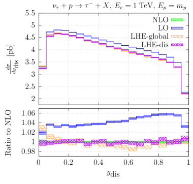
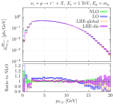
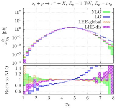
Figure 8: As in Fig 6 for the process $\nu_{\tau}+p\to\tau^{-}+X$.

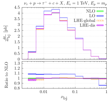
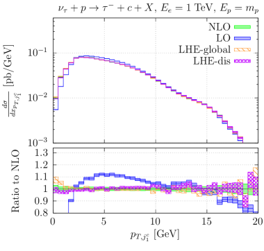
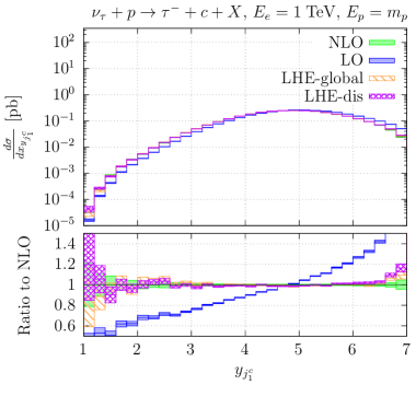
Figure 9: As in Fig 6 for the process $\nu_{\tau}+p\to\tau^{-}+c+X$. The leading jet $j_{1}^{c}$ is the leading charm-flavor jet.

• at LO (blue);

• at NLO (green);

• at the level of the POWHEG events (LHE) with the “global” option (orange);

• at the level of the POWHEG events with the “dis” option (purple).

The figures display statistical uncertainties as bands, while scale uncertainties are not taken into account.

Upon analyzing the first two curves, it is evident that NLO radiative corrections, while very mild for fiducial rates, can have a significant impact on more differential observables. Excluding the case of charm electro-production, it can be observed that NLO corrections have a similar pattern for all the considered processes. Specifically, the corrections have a significant impact on the shapes, including the DIS variable $x_{\rm bj}$, with the corrections reaching levels of $10-15\%$. The rapidity spectrum of the leading jet is particularly affected, with NLO corrections of about $50\%$ that shift the distribution towards smaller rapidities. Correspondingly, the $\Delta R_{j_{1},{\ell^{\prime}}}$ separation between the leading jet and the outgoing lepton shows a significant NLO correction, with a $30-40\%$ decrease at high values of separation. At LO, the leading jet and the outgoing lepton were back-to-back in the transverse plane, resulting in a $\Delta R_{j_{1},{\ell^{\prime}}}$ distribution that began at $\pi$. This restriction is lifted at NLO due to the additional real radiation.

As observed for the fiducial rates, when it comes to charm electro-production, NLO corrections lead to a significant increase in the normalisation corrections of approximately $50\%$. This increase can also be seen in the differential distributions, specifically in the $y_{\rm dis}$ distribution, where the $(1-y_{\rm dis})^{2}$ suppression of the LO result is clearly visible. The same suppression also plays a role in the rapidity distribution of the leading charm jet, and also in its transverse momentum for $p_{T,{j_{1}^{c}}}^{2}\lessapprox Q^{2}_{\rm min}$, where forward scattering is kinematically suppressed, while backward scattering is suppressed at LO, but becomes larger due to NLO corrections.

The transverse momentum distribution of the charm jet exhibits a distinctive change in slope at approximately $p_{T,{j_{1}^{c}}}=13\,\textrm{GeV}$. This effect is due to the different behavior of the dominant anti-strange and Cabibbo suppressed anti-down channels. The latter extends to higher $p_{T,{j_{1}^{c}}}$ values, resulting in a more gradual slope change beyond the kink point.

We will now compare the NLO results with the ones generated using the POWHEG formula at the event level, using the “global” (LHE-global) and “dis” (LHE-dis) settings for the mappings. It is important to remind that in the case of charm production, only the ISR region is present.

For the leptonic DIS observables we found, as expected, excellent agreement between NLO and LHE-dis, within their statistical uncertainties. Deviations of the LHE-global curves are mostly visible in the $x_{\rm bj}$ distribution, reaching a few tens of percent for $x_{\rm bj}<10^{-2}$. For jet observables, LHE-dis and LHE-global generally provide similar results, with mild deviations mostly seen in observables more sensitive to the extra radiation, such as the transverse momentum of the second jet $p_{T,j_{2}}$ and the $\Delta R_{j_{1},{\ell^{\prime}}}$ separation, especially in the region of small separations ($\Delta R_{j_{1},{\ell^{\prime}}}<\pi$).

When it comes to charm electro-production, the differences between LHE-global and LHE-dis results for the $x_{\rm bj}$ distribution are less noticeable compared to the massless quark cases. On the other hand, there are still approximately $5\%$ differences at high ${y_{\rm dis}}$. The reason behind the former observation, which is also valid in the case of charm neutrino-production, could be due to the fact that we are solely comparing the differences between the ISR dis mapping and the one that preserves the neutrino momentum and the invariant mass of the underlying Born system, while deviations caused by different mappings for FSR are expected to be larger.

We would like to briefly discuss the comparisons between the NLO results and the ones obtained at the event level. We will focus on the LHE-dis results and jet observables, as the leptonic variables are preserved by this choice of mappings. For leading order (LO) observables such as the transverse momentum and rapidity spectra of the leading jet, we observe a good agreement between NLO and LHE-dis results in the bulk, with some deviations towards small values of the transverse momentum and rapidity. The transverse momentum spectrum of the second jet, which is entirely due to real radiation, is divergent at NLO towards small values of transverse momentum. The LHE-dis result has a characteristic Sudakov suppression, forming a peak for transverse momenta of $p_{T,j_{2}}\gtrsim 1\,\textrm{GeV}$, where deviations from the fixed order result are at a level of around $20\%$. Then, the two results match at around $10\,\textrm{GeV}$. Other significant deviations between the NLO and LHE-dis results are present in the separation $\Delta R_{j_{1},{\ell^{\prime}}}$, near $\Delta R_{j_{1},{\ell^{\prime}}}=\pi$, a region which is sensitive to multiple soft emissions.

2.3 Comparison with NNLO

The option “dis” is the natural choice for lepton-hadron scattering processes. Parton shower programs implement recoil schemes that preserve lepton momenta, which means that predictions for the leptonic DIS variables will remain the same even after showering the POWHEG events. However, significant differences exist in the $x_{\rm bj}$ variables when using the “global” recoil as shown in the previous section. It is important to determine whether these differences are within the perturbative scale uncertainties. Additionally, NNLO radiative corrections may modify the leptonic variables. In the following, we compare the results obtained with the two mappings “dis” and “global”, including NLO scale variations, with available NNLO results.

For the massless case, we extend our structure function program to NNLO, thanks to the implementation of the higher-order proton structure functions in Hoppet Salam:2008qg ; hoppetv130 . The cross section for massive quark production in CC lepton-hadron scattering has been computed up to NNLO in QCD in ref. Berger:2016inr . The computation of the corresponding coefficient functions has been reported in ref. Gao:2017kkx . However, these results are not yet implemented in a publicly available tool. The coefficient functions for a massive quark have been previously computed at NNLO in the approximation of large momentum transfer, $Q^{2}\gg m_{Q}^{2}$, in ref. Buza:1996wv ; Blumlein:2014fqa . We rely on the latter for our comparison, as recently implemented in Yadism Candido:2024rkr .

We focus on the processes $e^{-}+p\to\nu_{e}+X$ and $e^{-}+p\to\nu_{e}+\bar{c}+X$, beginning with the massless case. The results for the leptonic variables Björken $x_{\rm bj}$ and ${y_{\rm dis}}$ are displayed in figure 10.

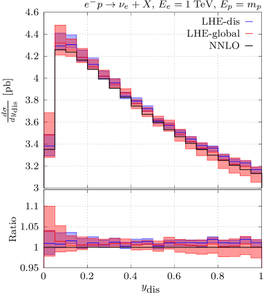
Figure 10: Leptonic kinematic distributions Björken $x_{\rm bj}$ (left) and ${y_{\rm dis}}$ (right) at the level of the POWHEG events with the “global” (LHE-global) and “dis” (LHE-dis) mappings. Scale uncertainties are shown as bands. Predictions at NNLO are reported for comparison. Ratios to NNLO are shown in the bottom panels.

The bands correspond to scale uncertainties computed by the customary seven-point scale variation around the reference scale $\mu^{2}_{F}=\mu^{2}_{R}=Q^{2}$. The Cabibbo angle is set to $\theta_{C}=0$ for this comparison. Upon inspection of the $x_{\rm bj}$ distribution, we observe that for $x_{\rm bj}\lesssim 0.01$, there are sizeable differences between the two recoil options, with their bands (of the order of $15-20\%$) barely overlapping. In this region, the NNLO prediction lies between the LHE-dis and LHE-global results. For larger $x_{\rm bj}$ values the three predictions are closer to each and the corresponding uncertainty bands are smaller, of the order of $5\%$, indicating good perturbative convergence in this region. In the case of the ${y_{\rm dis}}$ distribution, except for the first two bins, differences between the two mappings are very mild, around $1\%$, and are contained within the uncertainty bands, which are of the order of a few percent. The NNLO corrections are also mild and flat, reducing the NLO result by a few percent.

We turn now to the massive case, shown in figure 11.

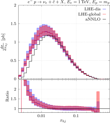
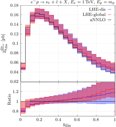
Figure 11: As figure 10 for charm electro-production in $e^{-}+p\to\nu_{e}+\bar{c}+X$. Approximate NNLO predictions are obtained with YadismCandido:2024rkr .

We observe an overall increase in the perturbative uncertainties and, correspondingly, larger NNLO effects. As observed and discussed in the previous section, differences between the predictions obtained with the two mappings are milder than those observed in the massless case. In the $x\gtrsim 0.01$ region, the approximate NNLO corrections are mild and flat, indicating good perturbative convergence. However, for $x<0.01$, they give a large negative contribution, causing the central aNNLO prediction to fall outside the NLO uncertainty bands. This region is associated with small values of the momentum transfer, and the approximation is expected to perform poorly in this regime. A more meaningful comparison would require the exact NNLO calculation, which we plan to investigate in future work.

Regarding the ${y_{\rm dis}}$ distribution, there is an overall better perturbative consistency as the aNNLO central prediction is mostly encompassed by the NLO uncertainties bands. The inclusion of aNNLO corrections brings a non-trivial shape distortion which leads to a sizeable softening the spectrum. At very high and very low ${y_{\rm dis}}$ values, the aNNLO effects can reach up to $15-20\%$. However, at very low ${y_{\rm dis}}$, the approximation is expected to worsen since this region probes small values of $Q^{2}$.

3 Pheno

In the previous section, we have introduced a new generator for NC and CC DIS lepton-nucleon processes reaching NLO+PS accuracy. In particular, we have discussed the impact of NLO corrections and some theoretical aspects related to the choice of the momentum mappings and their impact on differential distributions for the generated parton level events, before feeding them to a SMC program.

We now consider the full simulation chain including showering and hadronisation effects using PYTHIA8 Sjostrand:2014zea and adopting the recoil option SpaceShower:dipoleRecoil, which is suitable for DIS processes. We present a selection of comparisons with available data from electron(positron)-proton collisions at HERA as well as predictions for neutrino DIS processes for the ongoing FASER$\nu$ and SND@LHC, and for the upcoming SHiP experiments at CERN. For the latter case, we will briefly describe how to deal with a broad band beam of incoming neutrinos.

In particular, we focus on charm CC DIS production, either at the level of flavoured charm jet or at particle level of charmed mesons and baryons, and on the production of tau leptons in neutrino interactions. Charm CC DIS production is relevant for constraining the strange content of the proton. The current measurement with incoming charged leptons performed by the ZEUS collaboration ZEUS:2019oro is affected by large uncertainties, and the situation is expected to improve with the proposed EIC experiment Arratia:2020azl . On the other hand, for neutrino beams with an emulsion detector the identification of charm is topological, and thus has a very high efficiency and purity.

3.1 DIS in the forward region at HERA

In the following, we compare NLO+PS predictions with the single-jet measurements performed by the ZEUS collaboration for differential distributions in the laboratory frame ZEUS:2005ukc . The theory uncertainties on the predictions are obtained from the customary seven-point scale variation of renormalisation and factorisation scales around a central value of $\mu^{2}_{F}=\mu^{2}_{R}=Q^{2}$. We adopt the same physical parameters and pdf set as in Sec. 2.2.

The ZEUS measurement of differential distributions for jet production in the laboratory frame ZEUS:2005ukc is based on data that were taken colliding protons with energy of $E_{p}=820\,\textrm{GeV}$ and positrons with energy of $E_{e}=27.5\,\textrm{GeV}$, i.e. at a centre of mass energy of $\sqrt{s}=300.3\,\textrm{GeV}$. Jets are reconstructed using the $k_{T}$ clustering algorithm in the longitudinally invariant mode ($E_{T}$-weighted recombination scheme). The experimental analysis studied three regions of inclusive jet production in phase-space. We focus on the most inclusive region, called “global”. This region, which is expected to be well-described by the quark-model picture, is defined by the conditions

$$Q^{2}>25\,\textrm{GeV}^{2},\quad{y_{\rm dis}}>0.04,\quad E^{\prime}_{e}>10\,\textrm{GeV},$$ (12)

where $E^{\prime}_{e}$ is the energy of the scattered positron, and at least one jet satisfying

$$E_{\textrm{jet}}>6\,\textrm{GeV},\quad-1<\eta_{\textrm{jet}}<3.$$ (13)

We compare results at LO, NLO(LHE), LO+PS, and NLO+PS with the experimental measurements for the leading jet pseudo-rapidity ($\eta_{j}$) and transverse energy ($E_{T,j}$), momentum transfer ($Q^{2}$), and Björken variable ($x_{\rm bj}$), as shown in figure 12. For a meaningful comparison with data provided at the particle level, predictions obtained through matching to the parton shower are required. Results at LO and NLO(LHE) are displayed for reference only. At NLO+PS level, we achieve a much-improved description of the data, with significantly reduced scale uncertainty bands and central values closer to the experimental data in the regions where we expect an improvement. Examples of a kinematic domain where a good agreement is not expected are provided by the lower-order suppressed regions of high jet pseudo rapidities ($\eta_{j}\gtrsim 1.5$), and of the small $x_{\rm bj}$ values ($x_{\rm bj}\lesssim 10^{-3}$). In fact, these are still not accurately described even with the addition of the first extra emission, which is given by the exact matrix element in the NLO(LHE) and NLO+PS predictions and approximated by the shower in the LO+PS one. Higher-order corrections are necessary for these regions. The authors of ref. Currie:2018fgr performed a calculation of the DIS single-jet inclusive production up to N³LO in QCD based on the projection to Born method Cacciari:2015jma and obtained an excellent description of the ZEUS data in the “global” region. However, their predictions are at the parton level, and to make a meaningful comparison with the data, the experimental results have been unfolded from particle to parton level.

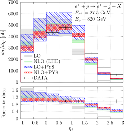
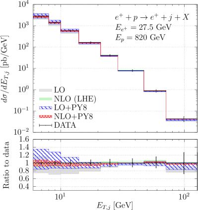
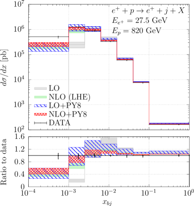
Figure 12: Comparisons of theoretical predictions at LO (in gray), NLO (LHE) (in green), LO+PS (in blue) and NLO+PS (in red) with ZEUS measurements ZEUS:2005ukc for kinematic distributions in single inclusive jet production: the leading jet pseudo-rapidity ($\eta_{j}$) and transverse energy ($E_{T,j}$), momentum transfer ($Q^{2}$), and Björken variable ($x_{\rm bj}$). LO+PS and NLO+PS are matched to PYTHIA8 shower. Ratios to data are displayed in the bottom panels.

3.2 Charm CC electro-production at HERA

The production of charm in CC DIS results in smaller cross sections compared to NC DIS and photoproduction. This makes measuring charm production more challenging. However, it is an interesting process because it helps constrain the strange content of the probed nucleon. The first measurement of charm production in CC DIS was carried out by the ZEUS collaboration ZEUS:2019oro , using HERA data in $e^{\pm}p$ collisions at a centre-of-mass energy of $\sqrt{s}=318\;$GeV. Although the measurement was affected by large statistical uncertainties, it is an important step towards better understanding charm production in CC DIS.

The charm cross section has been measured in the kinematic phase space region defined by the requirements

$$200\,\textrm{GeV}^{2}<Q^{2}<60000\,\textrm{GeV}^{2},\quad{y_{\rm dis}}<0.9\;,$$ (14)

into two $Q^{2}$ bins: $200\,{\rm{GeV}}^{2}<Q^{2}<1500\,{\rm{GeV}}^{2}$ and $1500\,\textrm{GeV}^{2}<Q^{2}<60000\,\textrm{GeV}^{2}$. Moreover, a region for the visible charm jet has been defined by imposing

$$E^{\rm jet}_{T}>5\,{\rm GeV},\quad-2.5<\eta<2.0$$ (15)

on the identified charm jet, where the jets are reconstructed with the $k_{T}$ clustering algorithm with a radius parameter $R=1$ in the longitudinally invariant mode and adopting the $E$-recombination scheme.

In table 2 we report LO+PS and NLO+PS predictions obtained in the fixed-flavour-number scheme with $n_{f}=3$ light quarks and a massive charm for both the charm and the visible charm-jet cross sections in the two $Q^{2}$ bins. We set the charm mass to $m_{c}=1.28\,$GeV and adopt the ABMP16.3 Alekhin:2012ig ; Bierenbaum:2009zt PDF set. Our calculation does not include a significant contribution due to diagrams with a gluon splitting $g\to c\bar{c}$, which are $\mathcal{O}(\alpha_{s}^{2})$ terms. These contributions are usually considered as background to the so-called EW component of the charm production in CC DIS since they are dominated by valence densities. The EW component, in contrast, is directly sensitive to the strange density.

Upon inspection of table 2,

	$\sigma^{e^{+}p}_{c,\rm{vis}}$ [pb]			$\sigma^{e^{+}p}_{c}$ [pb]
$Q^{2}$ range (GeV2)	LO+PS	NLO+PS	ZEUS	LO+PS	NLO+PS	ZEUS
$200-1500$	$2.085_{-6.2\%}^{+4.7\%}$	$2.501_{-3.7\%}^{+4.8\%}$	$4.1\pm 2.0$	$2.657_{-4.5\%}^{+3.3\%}$	$4.248_{-4.3\%}^{+5.7\%}$	$8.7\pm 4.1$
$1500-60000$	$0.9921_{-1.5\%}^{+1.3\%}$	$1.028_{-5.1\%}^{+6.9\%}$	$-0.7\pm 2.0$	$1.157_{-2.2\%}^{+2.2\%}$	$1.604_{-6.2\%}^{+8.2\%}$	$-1.2\pm 3.9$

Table 2: LO+PS and NLO+PS predictions for charm production cross sections in CC DIS $e^{+}p$ at HERA within the kinematic phase space defined in eq. (14). The visible cross sections refer to the additional visibility cuts on the charm jet in eq. (15). Corresponding cross sections measured by the ZEUS collaboration ZEUS:2019oro are also reported.

we see that radiative corrections have a more significant impact on the first $Q^{2}$ bin at lower $Q^{2}$ values and in the more inclusive setup compared to the visible charm-jet region. For the more inclusive region, they reach up to $+60\%(+45\%)$ in the first(second) bin in $Q^{2}$, with no overlap between the LO+PS and NLO+PS results. The slightly larger correction in the first bin is related to larger values of $\alpha_{s}$ at smaller scales. The NLO corrections turn out to be smaller when applying the visibility cuts on the charm jet. This is likely due to the fact that these cuts affect the population of large ${y_{\rm dis}}$ region, that for charm electro-production gets larger positive NLO corrections, as already discussed in the previous section.

Scale uncertainties are obtained by independently varying the renormalisation $\mu_{R}$ and factorisation $\mu_{F}$ scales around the central reference scale $\mu_{0}=\sqrt{Q^{2}+m_{c}^{2}}$ by a factor of two up and down, with the additional constraint $1/2<\mu_{R}/\mu_{F}<2$. The results obtained from LO calculations tend to underestimate the rates and corresponding theoretical uncertainties. The inclusion of higher-order corrections is, therefore, necessary.

3.3 DIS with a neutrino flux

We start by considering a flux of incoming neutrinos given as a binned histogram of the neutrino energy in the laboratory frame of the $\nu N$ collision. In particular, the histogram defines the normalised flux function $f$ as

$$f(E_{\nu}^{\rm{lab}})=\frac{1}{N}\frac{\mathrm{d}N}{\mathrm{d}E_{\nu}^{\rm{lab}}}.$$ (16)

Defining $E_{\nu}^{\rm{max,lab}}$ as the energy of the most energetic neutrino in the flux, each neutrino involved in the scattering process can be thought as carrying a fraction $x=E_{\nu}^{\rm{lab}}/E_{\nu}^{\rm{max,lab}}$ of the maximal energy of the beam. Furthermore we set as reference frame the CM of $\nu$ with energy $E_{\nu}^{\rm{max,lab}}$ and the nucleon at rest. We then define

$$S_{H}=M^{2}+2ME_{\nu}^{\rm{max,lab}},$$ (17)

with $M$ denoting the mass of the nucleon. The maximum neutrino energy in the reference frame is then

$$E_{\nu}^{\rm{max,CM}}=\frac{S_{H}-M^{2}}{2\sqrt{S_{H}}}.$$ (18)

We then define a neutrino beam density function (BDF) as

$$f_{\nu}(x)\equiv\frac{1}{N}\frac{\mathrm{d}N}{\mathrm{d}E_{\nu}^{\rm{lab}}}E_{\nu}^{\rm{max,lab}}=\frac{1}{N}\frac{\mathrm{d}N}{\mathrm{d}x}.$$ (19)

This is now the boost invariant neutrino BDF we need. Since SMC programs normally deal with a fixed-energy lepton-nucleon interaction, some extra care is needed when interfacing them with POWHEG.

3.4 Setup

We consider three case studies: the SND@LHC, SHiP and FASER$\nu$ experiments. For all these applications with neutrino fluxes we have used the setup of section 2.2, except that the cut in $Q^{2}$ has been set to $Q^{2}>2\,$GeV². The standard seven-point scale variation will also be shown in all plots. Furthermore, having all the three experiments a tungsten target, we separately computed the cross section for scattering off protons and neutrons and combined the results to build the cross section per tungsten nucleon, that will be denoted as $n_{t}$ in the plots.

3.5 $\tau$ neutrinos at SND@LHC

As an illustrative example of the computation of fully differential deep inelastic scattering cross sections initiated by a flux of neutrinos with variable energy we consider the charged current $\tau$ neutrino and anti-neutrino interactions at SND@LHC. We have used the normalized flux simulated by the SND@LHC collaboration SNDLHC:2022ihg , which we show in figure 13.

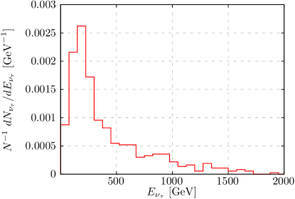
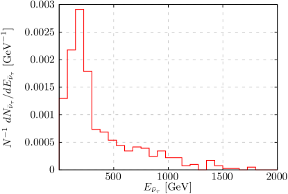
Figure 13: Normalized energy flux of $\nu_{\tau}$ (left panel) and ${\bar{\nu}_{\tau}}$ (right panel) entering the SND@LHC target.

Here and in the following we assume no errors on the fluxes, that are thus given as step functions.

In figure 14 we show the cross sections

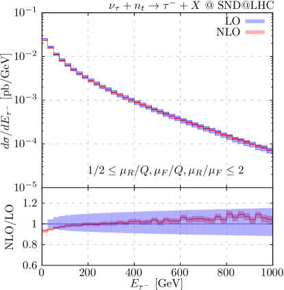
Figure 14: Energy distribution of $\tau^{-}(\tau^{+})$ produced in charged current $\nu_{\tau}\leavevmode\nobreak\ (\bar{\nu}_{\tau})$ scattering at the SND@LHC target per tungsten nucleon.

per tungsten nucleon as a function of the energy of the produced $\tau$ lepton. NLO corrections are negative and about -5% in the dominant small energy region, and mildly rise with energy reaching +5% (+10%) for 1 TeV $\tau$ (${\bar{\tau}}$) lepton. The scale uncertainties are strongly reduced but in the very first bin where the NLO results lay outside of the LO bands.

3.6 $\tau$ neutrinos at SHiP

We evaluated the DIS cross section induced by an incoming flux of $\tau$ neutrinos and anti-neutrinos interacting in the SHiP target. The fluxes shown in figure 15 have been generated by the SHiP collaboration SHiP:2015vad . In figure 16 we show the cross

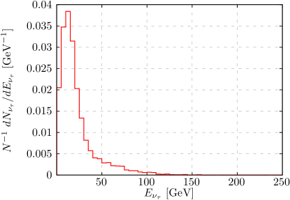
Figure 15: Normalized energy flux of $\nu_{\tau}$ (left panel) and ${\bar{\nu}_{\tau}}$ (right panel) entering the SHiP target.

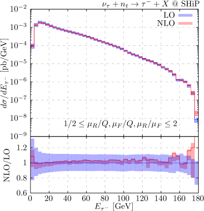
Figure 16: Energy distribution of $\tau^{-}\leavevmode\nobreak\ (\tau^{+})$ produced in charged current $\nu_{\tau}\leavevmode\nobreak\ (\bar{\nu}_{\tau})$ scattering at the SHiP target per nucleon of Tungsten.

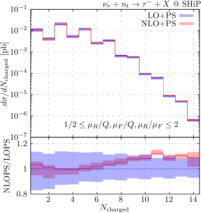
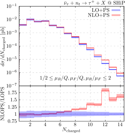
Figure 17: Charged particle multiplicity produced in charged current $\tau$ (anti-)neutrino scattering at the SHiP target per nucleon of tungsten.

section per nucleon as a function of the energy of the produced charged lepton. Here (and in general also in the following plots) the radiative corrections reduce considerably the uncertainty band, becoming non negligible only for very small and very large energies.

By matching our fixed-order computation with PYTHIA8 we evaluated several kinematic distributions of variables used to describe the hadronic final state. We start by showing cross sections as function of the number of charged particles in the final state after the shower and hadronisation process. We observe that the NLO corrections tend to increase the multiplicities of charged particles, especially for the incoming anti-neutrino. We also observe the alternating behaviour of the cross section for even-odd multiplicities. This is explained by the fact that for proton target the multiplicity must be even (for charge conservation), while for neutron target it must be odd. The tungsten nucleon is a mixture of the two, with a large prevalence of the neutron. In neutrino scattering the target down quarks prevail by far, because we have more neutrons and the neutrons have more down quarks. In the anti-neutrino scattering off protons an up quark must be hit, thus yielding a cross section larger by about a factor of two with respect to the neutron case, nearly compensating the larger neutron fraction. Thus the strong prevalence of the odd multiplicity for neutrinos, and, as can be seen in the figure, a very slight prevalence of even multiplicities for anti-neutrinos.

In fig. 18 we show the cross section as a

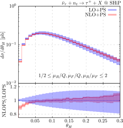
Figure 18: Scattering angle of the hadronic final-state system produced in charged current $\nu_{\tau}$ ($\bar{\nu}_{\tau}$) scattering at SHiP target per nucleon of tungsten.

function of the scattering angle $\theta$ of the hadronic final system in the laboratory frame, for both $\tau$ neutrino and anti-neutrino scattering. Here we observe a strong reduction of the scale uncertainty but also regions where the NLO+PS band is not contained in the LO+PS one. For an incoming neutrino the radiative corrections have an effect between -5% up to 10%. A similar pattern can be observed for an incoming anti-neutrino, except for the larger negative NLO corrections at small angles.

In fig. 19 we show the cross section as a function

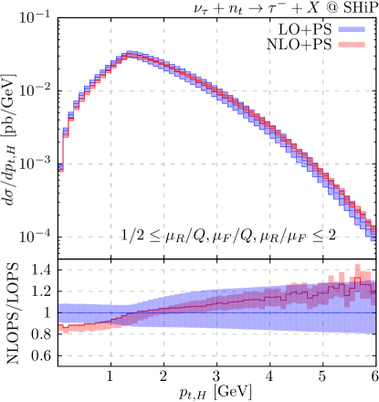
Figure 19: As in fig. 18 for the transverse momentum.

of the transverse momentum of the hadronic final state, either for an incoming tau neutrino flux (left panel), or for an anti-neutrino flux (right panel). We see a similar pattern in both cases. Looking at $p_{t}>1\,$GeV we observe that the radiative corrections are relatively small and contained in the LO+PS band. Below the cusp, at roughly $p_{t}=\sqrt{2}\,$GeV, the cross sections are affected by the $Q^{2}$ cut, and show a different pattern. We also see a noticeable change of shape induced by the NLO corrections.

Finally, in fig. 20 we show the cross section as a

Figure 20: As in fig. 19 for the transverse momentum of produced $\pi^{+}$ for an incoming $\nu_{\tau}$ ($\bar{\nu}_{\tau}$) flux.

function of the transverse momentum of inclusively produced positively charged pions. NLO corrections are mild in the whole range, with the NLO bands contained in the LO ones in the whole $p_{t}$ range that we have explored.

3.7 Charm production at FASER$\nu$

We have computed the cross section for charm production in muon neutrino and anti-neutrino CC scattering at FASER$\nu$ using the fluxes predicted in Buonocore:2023kna ; FASER:2024ykc and shown in fig. 21.

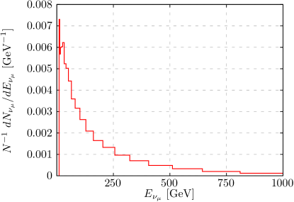
Figure 21: Number of $\nu_{\mu}$ (left panel) and ${\bar{\nu}_{\mu}}$ (right panel) entering the FASER$\nu$ target per bin of $\nu$ energy in the laboratory frame.

In figures 22 and 23 the energy

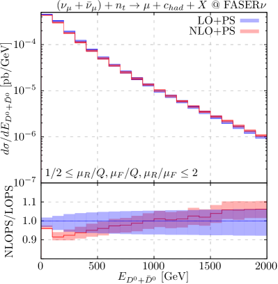
Figure 22: Energy distribution of charged (left) and neutral (right) $D$ mesons produced via charged current $\nu_{\mu}+{\bar{\nu}}_{\mu}$ events in FASER$\nu$.

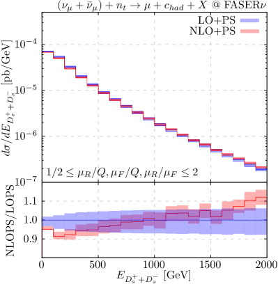
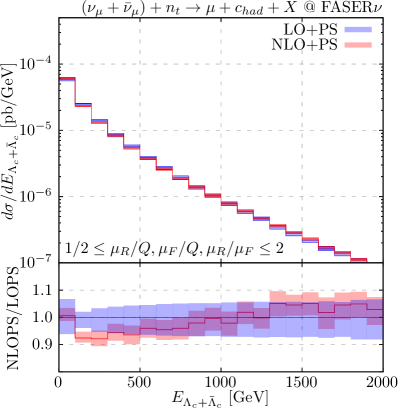
Figure 23: Energy distribution of $D_{s}$ (left) and $\Lambda_{c}$ (right) particles and antiparticles produced via charged current $\nu_{\mu}+{\bar{\nu}}_{\mu}$ events in FASER$\nu$.

distributions of charmed mesons and $\Lambda_{c}$ are shown. Generally speaking, we see that the NLO corrections lead to a hardening of all distributions.

4 Conclusions

In this paper we have presented a new POWHEG event generator to describe deep inelastic lepton hadron scattering at NLO+PS accuracy. Our code produces results for charged current as well as neutral current processes initiated by a massless lepton. The final state lepton and quark can be massless or massive. To build our code we have developed and implemented new FKS phase space mappings for initial and final state radiation, that preserve the leptonic variables and are suitable for the case of massive particles in the final state. These mappings, described in detail in the appendices, smoothly adapt when the final state particles are massless.

We have validated our NLO computation through a tuned comparison with an in house code based upon the DIS lepton hadron cross section expressed in terms of form factors, which we computed convoluting PDFs with the NLO coefficient functions.

We have studied the impact of the NLO corrections for the different possible final states, and the impact of the matching procedure focusing especially on the (sub-leading) effects related to the choice of the momentum mapping.

We also compared the prediction of our code for the lepton distributions with available higher order corrections. In order to do this we extended our in house code by including NNLO form factors available in Hoppet for the case of a massless final state quark, and, for a massive quark, using the approximate NNLO result implemented in Yadism Candido:2024rkr .

Having implemented and validated our code, we have shown some illustrative applications. We first compared our results with two analyses at HERA, one for charged current $ep$ scattering, and one focusing on single charm production. Then we moved to incoming neutrino beams, showing predictions for charm and tau lepton yields at the ongoing experiments FASER$\nu$ and SND@LHC, and at the upcoming SHiP experiment. In order to run with broad band beams of neutrinos in the initial state one has to provide a binned histogram with the neutrino flux, that we have taken from available studies.

Other studies can be easily implemented for past experiments, like the study of associated charm production in NC $ep$ scattering at HERA, or future DIS studies at the proposed EIC experiment. Furthermore, our tool may be used in the context of tau neutrino appearance in atmospheric neutrino oscillations, see e.g. IceCube:2019dqi , or to include mass effects in top CC DIS production with very high energy neutrinos from cosmic rays Cooper-Sarkar:2011jtt ; Garcia:2020jwr .

Our tool will be soon made publicly available in the POWHEG-BOX repository.

We conclude by noticing that, being based on the POWHEG-BOX framework, our work can be extended in several directions. NLO electroweak corrections can be included, and also the NLO QCD corrections can be extended with one extra radiated parton in the final state. This would allow to promote the computation to NNLO+PS via a MiNNLO Hamilton:2012rf ; Hamilton:2013fea ; Monni:2019whf procedure.

Appendix A Mappings for DIS

A.1 Conventions

The deep inelastic scattering process proceeds at LO via the parton reaction

$$\ell(l)+q(\bar{x}P)\to{\ell^{\prime}}({l^{\prime}})+q\prime(v),$$ (20)

where $P$ is the incoming nucleon momentum and, in general, the final-state lepton and quark can be massive, ${l^{\prime}}^{2}=m_{{\ell^{\prime}}}^{2}$ and $v^{2}=m_{v}^{2}$. In the following, we will always assume that the nucleon is coming from the positive $z$-axis direction. The corresponding Born phase space element is

$$\mathrm{d}{\bf{\Phi}}_{B} =\mathrm{d}\bar{x}\frac{\mathrm{d}^{3}{l^{\prime}}}{2{l^{\prime}}^{0}(2\pi)^{3}}\frac{\mathrm{d}^{3}v}{2v^{0}(2\pi)^{3}}(2\pi)^{4}\delta^{(4)}(l+\bar{x}P-{l^{\prime}}-v)$$ (21)

$$=\mathrm{d}\bar{x}\frac{\mathrm{d}^{3}{l^{\prime}}}{4{l^{\prime}}^{0}v^{0}(2\pi)^{2}}\delta(\sqrt{\bar{x}S}-{l^{\prime}}^{0}-v^{0})$$ (22)

$$=\frac{1}{16\pi^{2}}\mathrm{d}\bar{x}d{y_{\rm dis}}d\phi_{{l^{\prime}}},$$ (23)

in terms of the $y\equiv{y_{\rm dis}}$ and $\bar{x}\equiv x_{\rm bj}$ variables defined in eq. (3), $\phi_{{l^{\prime}}}$, the azimuthal angle of the outgoing lepton in a given reference frame, and $S=(l+P)^{2}$ is the total energy of the lepton-nucleon collision. At NLO, the real emission processes

$$\ell(l)+q(xP) \to{\ell^{\prime}}({l^{\prime}})+q\prime(v)+g(k),$$ (24)

$$\ell(l)+g(xP) \to{\ell^{\prime}}({l^{\prime}})+q\prime(v)+\bar{q}(k).$$ (25)

must be taken into account. The real emission phase space reads

$$\mathrm{d}{\bf{\Phi}}_{R}=\mathrm{d}x\frac{\mathrm{d}^{3}{l^{\prime}}}{2{l^{\prime}}^{0}(2\pi)^{3}}\frac{\mathrm{d}^{3}v}{2v^{0}(2\pi)^{3}}\frac{\mathrm{d}^{3}k}{2k^{0}(2\pi)^{3}}(2\pi)^{4}\delta^{(4)}(l+\bar{x}P-{l^{\prime}}-v-k).$$ (26)

The corresponding matrix elements develop singularities in the limit of soft and/or collinear emission. In what follows we will show how to construct a mapping from the real phase space ${\bf{\Phi}}_{R}$ to the underlying Born variables (and its corresponding inverse mapping) for the two kinds of singular regions, namely the initial and final state ones. We will consider mappings compatible with the FKS Frixione:1995ms subtraction method.

A.2 Momentum mappings for DIS

A.2.1 DIS momentum mapping preserving the invariant mass of the born-like lepton-quark system

We start by considering the mapping associated to the initial-state singular region. We notice that the standard POWHEG mapping introduced in ref. Frixione:2007vw cannot be applied to the DIS kinematics as the longitudinal recoil of the emitted parton is reabsorbed by both initial state partons. In this way, the mapping preserves both the rapidity and the invariant mass of the Born system. In this section, we will show a simple modification of that construction that does not change the momentum of the incoming lepton.

Following the FKS formulation, we work in the rest frame of $l+xP$, i.e. the partonic CM frame of the real configuration, and we introduce the standard FKS variables

$$\quad\xi=\frac{2k\cdot(l+p)}{(l+p)^{2}},\quad y=\cos\theta_{k},\quad\phi$$ (27)

for the case of ISR radiation. The angles $\theta_{k}$ and $\phi$ are relative to the positive beam axis direction. In this parametrisation, the momentum $k$ reads

$$k=\frac{\sqrt{xS}}{2}\xi(1,\sin{\theta}\sin{\phi},\sin{\theta}\cos{\phi},\cos{\theta}),$$ (28)

and the corresponding one-particle phase space element is

$$\frac{\mathrm{d}^{3}k}{2k^{0}(2\pi)^{3}}=\frac{xS}{(4\pi)^{3}}\xi\mathrm{d}\xi\mathrm{d}y\mathrm{d}\phi.$$ (29)

We introduce the momentum of the Born final state

$$k_{\rm{tot}}=l+xP-k=\frac{\sqrt{xS}}{2}(2-\xi,-\xi\sin{\theta}\cos{\phi},-\xi\sin{\theta}\sin{\phi},-\xi\cos{\theta}).$$ (30)

Following the standard POWHEG construction we reabsorb the longitudinal and transverse momentum by performing a sequence of boost transformations

$$\bar{k}_{\rm tot}=B^{-1}_{\parallel}B_{\perp}B_{\parallel}k_{\rm tot},$$ (31)

consisting in a longitudinal boost to the system of zero rapidity of $k_{\rm tot}$, a transverse boost in order to absorb its transverse component and, finally, the inverse of the longitudinal boost. By construction, the invariant mass of the Born final-state system $\bar{k}_{\rm tot}^{2}=k^{2}_{\rm tot}$ is preserved. We require now that

$$\bar{k}_{\rm tot}=l+\bar{x}P,$$ (32)

which, at variance with the standard POWHEG construction, implies that we cannot also preserve the rapidity of the Born system. From the conservation of the invariant mass, we immediately obtain an expression of the underlying Born momentum fraction $\bar{x}$ in terms of the radiation variables and $x$

$$(l+xP-k)^{2}=(l+\bar{x}P)^{2}\implies xS(1-\xi)=\bar{x}S\implies\bar{x}=(1-\xi)x.$$ (33)

The inverse mapping, consisting in reconstructing the kinematic of the real emission from the underlying Born momenta and the radiation variables $\xi$, $y$ and $\phi$, can be easily obtained by inverting eq. (33)

$$x=\frac{\bar{x}}{1-\xi},$$ (34)

and eq. (31).

Requiring $x\leq 1$ we also obtain an upper bound for the energy fraction of the emitted parton

$$\xi\leq 1-\bar{x}\equiv\xi_{\rm{max}}.$$ (35)

The real emission phase space element reads

$$d{\bf\Phi}_{R}=\mathrm{d}\bar{x}d\Phi_{B}\frac{\bar{x}S}{(4\pi)^{3}}\xi\mathrm{d}\xi\mathrm{d}y\mathrm{d}\phi\equiv\mathrm{d}\bar{x}d\Phi_{B}J(\xi,y,\phi;\bar{x})\mathrm{d}\xi\mathrm{d}y\mathrm{d}\phi$$ (36)

from which we get the jacobian of the mapping

$$J(\xi,y,\phi;\bar{x})=\frac{\bar{x}S}{(4\pi)^{3}}\xi.$$ (37)

A.2.2 DIS momentum mapping preserving the lepton kinematics: the ISR case

A more interesting option is to set up a projection from a real phase space configuration to an underlying Born one that preserves the momentum of the scattered lepton. In this case, both ${y_{\rm dis}}$ (or $Q^{2}$) and $x_{\rm bj}$ remain invariant, that is a natural choice for this process.

Consider the system in the lepton-proton CM. Let us call $E$ the energy of the incoming proton and lepton, $E^{\prime}$ the energy of the outgoing lepton, and $\theta$ the lepton scattering angle. Retaining the dependence on the mass of the outgoing lepton, $m_{{\ell^{\prime}}}$, we have

$$Q^{2} = -(l-{l^{\prime}})^{2}=-m^{2}_{{\ell^{\prime}}}+2l\cdot{l^{\prime}}=-m^{2}_{{\ell^{\prime}}}+2EE^{\prime}(1-\beta^{\prime}\cos\theta),$$ (38)

$$\nu = (l-{l^{\prime}})\cdot P=2E^{2}-EE^{\prime}(1+\beta^{\prime}\cos\theta),$$ (39)

where $\beta^{\prime}=|\vec{{l^{\prime}}}|/E^{\prime}$. Then, it follows that both $E^{\prime}$ and $\theta$ must remain fixed to preserve $x_{\rm bj}$ and $Q^{2}$. At the Born level, the struck parton carries a fraction $\bar{x}$ of the incoming proton momentum $P$. We consider the general case of producing a massive final-state quark of momentum $v$ and mass $m_{v}$. By imposing the on-shell condition on the scattered quark momentum, we get $v=l-{l^{\prime}}+\bar{x}P=q+\bar{x}P$

$$v^{2}=-Q^{2}+2\bar{x}\nu=m_{v}^{2}\implies\bar{x}=\frac{Q^{2}+m_{v}^{2}}{2\nu}$$ (40)

which reduces to $x_{\rm bj}$ in the limit of a massless outgoing quark. If a gluon with momentum $k$ is emitted, the momentum fraction $x$ associated to the real configuration can be similarly computed starting from $v=q+xP-k$ and imposing that $v$ is on the mass shell. We get

$$x=\frac{Q^{2}+m_{v}^{2}+2k\cdot q}{2(\nu-k\cdot P)}.$$ (41)

In particular, we notice that if $k$ is collinear to $P$, say $k=\xi p$, we have

$$x=\frac{Q^{2}+m_{v}^{2}+2\xi\nu}{2\nu}=\bar{x}+\xi,$$ (42)

as expected. Again, we work in the rest frame of $l+p$ with $p=xP$ and introduce standard FKS variables as in eq. (27). Then, the kinematics is given by

$$l = \frac{\sqrt{s}}{2}(1,0_{\perp},1),$$ (43)

$$p = \frac{\sqrt{s}}{2}(1,0_{\perp},-1),$$ (44)

$$k = \xi\frac{\sqrt{s}}{2}\left(1,\sqrt{1-y^{2}}s_{\phi},\sqrt{1-y^{2}}c_{\phi},y\right)\;,$$ (45)

where $s=(l+p)^{2}$, $s_{\phi}\equiv\sin\phi$ and $c_{\phi}\equiv\cos\phi$. We observe that the relevant initial state collinear limit corresponding to the emitted gluon being collinear to the incoming quark is approached for $y\to-1$. It is convenient to write the momentum of the final-state lepton ${l^{\prime}}$ in terms of $Q^{2}$, $\nu$ and $S=(l+P)^{2}$, which are preserved by the mapping, and of the momentum fraction $x$. To this end, we start from the following parametrisation

$${l^{\prime}}={l^{\prime}}^{0}(1,\beta^{\prime}\sin\theta^{\prime},0,\beta^{\prime}\cos\theta^{\prime}),$$ (46)

where, without loss of generality, we set the azimuth of the final-state lepton to zero. Then, the invariants $Q^{2}$ and $\nu$ can be written as

$$Q^{2} = -m_{{\ell^{\prime}}}^{2}+\sqrt{s}{l^{\prime}}^{0}(1-\beta^{\prime}\cos\theta^{\prime}),$$ (47)

$$2\nu = S-\frac{\sqrt{s}}{x}{l^{\prime}}^{0}(1+\beta^{\prime}\cos\theta^{\prime}).$$ (48)

Inverting the above system in terms of the variables ${l^{\prime}}^{0}$ and $\beta^{\prime}\cos\theta^{\prime}$, we obtain

$${l^{\prime}}^{0} = \frac{Q^{2}+m_{\ell^{\prime}}^{2}+(S-2\nu)x}{2\sqrt{s}}=\frac{Q^{2}+m_{{\ell^{\prime}}}^{2}}{2\sqrt{s}}\left(1+\frac{x}{\chi}\right),$$ (49)

$$\beta^{\prime}\cos\theta^{\prime} = 1-2\frac{Q^{2}+m_{\ell^{\prime}}^{2}}{Q^{2}+m_{\ell^{\prime}}^{2}+(S-2\nu)x}=\frac{x-\chi}{x+\chi}.$$ (50)

where we have introduced the quantity

$$\chi\equiv\frac{Q^{2}+m_{\ell^{\prime}}^{2}}{S-2\nu}=x\frac{1-\beta^{\prime}\cos\theta^{\prime}}{1+\beta^{\prime}\cos\theta^{\prime}}.$$ (51)

In summary, we have

$${l^{\prime}}=\frac{Q^{2}+m_{\ell^{\prime}}^{2}}{2\chi\sqrt{s}}\left[x+\chi,2\sqrt{\chi x-\frac{\chi^{2}m_{\ell^{\prime}}^{2}s}{(Q^{2}+m_{\ell^{\prime}}^{2})^{2}}},0,x-\chi\right].$$ (52)

The momentum of the final-state quark is then fixed by momentum conservation to be $v=q+p-k$. In this way, we have constructed a mapping from a given Born phase space point and radiation variables $\xi,y,\phi$ to a real one under the assumption that eq. (41) admits at least one solution. Indeed, $x$ must satisfy the equation

$$0 = \left[{\tilde{S}}\xi(1+y)-4\nu(1-\xi)\right]x+\left[2s_{\phi}\xi\sqrt{\left({\tilde{S}}Q^{2}-2\nu m_{\ell^{\prime}}^{2}\right)(1-y^{2})}\right]\sqrt{x}$$ (53)

$$+4\nu\bar{x}-(Q^{2}+m_{\ell^{\prime}}^{2})\xi(1+y)\equiv{a_{x}}x+{b_{x}}\sqrt{x}+{c_{x}}.$$

where ${\tilde{S}}=S-2\nu$. Notice that the dependence on the mass of the final-state quark is implicitly contained in the Born momentum fraction $\bar{x}$. In the soft limit $\xi=0$, the equation becomes

$$4\nu(-x+\bar{x})=0\Rightarrow x=\bar{x}.$$ (54)

as it should. We look after solutions in the physical range $[\bar{x},1]$ of eq. (53), which is quadratic in $\sqrt{x}$. At fixed underlying Born configuration, this leads to non trivial boundaries in the radiation phase space $[0,1]_{\xi}\times[-1,1]_{y}\times[0,2\pi]_{\phi}$. In order to have real solution, the discriminant of eq. (53) must be positive:

$$\Delta_{x} = 4\left[({\tilde{S}}Q^{2}-2m_{\ell^{\prime}}^{2}\nu)s_{\phi}^{2}(1-y)+(Q^{2}+m_{\ell^{\prime}}^{2})(4\nu+{\tilde{S}}(1+y))\right](1+y)\xi^{2}$$ (55)

$$-16\nu\left[4\nu\bar{x}+(Q^{2}+m_{\ell^{\prime}}^{2}+{\tilde{S}}\bar{x})(1+y)\right]\xi+64\nu^{2}\bar{x}$$

$$\equiv {a_{\xi}}\xi^{2}+{b_{\xi}}\xi+{c_{\xi}}>0$$

We employ the above condition to derive constraints on the $\xi$ variable as function of the underlying Born and the other two radiation variables $y$ and $\phi$. Eq. (55) is quadratic in $\xi$ with a clearly positive coefficient of the $\xi^{2}$ term as the quantity $({\tilde{S}}Q^{2}-2m_{\ell^{\prime}}^{2}\nu)\geq 0$ in the $2\to 2$ Born kinematics. In order to study if there are real solutions, we evaluate its discriminant

$$\Delta_{\xi} = (16\nu)^{2}\left[((Q^{2}+m_{\ell^{\prime}}^{2}-{\tilde{S}}\bar{x})(1+y)-4\nu\bar{x})^{2}-4s_{\phi}^{2}\bar{x}({\tilde{S}}Q^{2}-2m_{\ell^{\prime}}^{2}\nu)(1-y^{2})\right]$$ (56)

$$\geq (16\nu)^{2}\left[((Q^{2}+m_{\ell^{\prime}}^{2}-{\tilde{S}}\bar{x})(1+y)-4\nu\bar{x})^{2}-4\bar{x}({\tilde{S}}Q^{2}-2m_{\ell^{\prime}}^{2}\nu)(1-y^{2})\right],$$

being the coefficient of $s_{\phi}^{2}$ negative. The quantity in the square bracket is a quadratic polynomial in $y$ that is equal to $16\nu^{2}x_{b}^{2}>0$ at $y=-1$ and, as its discriminant is negative

$$\Delta_{y}=-64S\bar{x}^{2}m_{v}^{2}({\tilde{S}}Q^{2}-2m_{\ell^{\prime}}^{2}\nu)<0,$$ (57)

it is positive definite. Therefore, we conclude that $\Delta_{\xi}>0$, there are always two real solutions $\xi_{1}<\xi_{2}$ and $\Delta$ is positive for $\xi\leq\xi_{1}$ or $\xi\geq\xi_{2}$ in the allowed range $[0,1]_{\xi}$. Furthermore:

1. the coefficients of the quadratic polynomial in $\xi$ in eq. (55) have definite signs and it follows that $\xi_{1}>0$ ( ${a_{\xi}}>0$, ${b_{\xi}}<0$ and ${c_{\xi}}>0$ );

2. the upper limit for $\xi=1$ corresponds to the condition ${a_{\xi}}+{b_{\xi}}+{c_{\xi}}=0$. Solving it with respect to $y$, we obtain two solutions

   $$y_{1}=-1,\quad\quad y_{2}=1+2\frac{{\tilde{S}}(m_{v}^{2}-m_{\ell^{\prime}}^{2})}{{\tilde{S}}(Q^{2}+m_{\ell^{\prime}}^{2})-({\tilde{S}}Q^{2}-2m_{\ell^{\prime}}^{2}\nu)s_{\phi}^{2}}.$$ (58)

3. We consider first the solution $y_{1}$. We observe that $\xi_{1}=1$ at $y=y_{1}$ independently of the Born kinematics and $\phi$. Being $\xi_{2}>\xi_{1}$, the second solution leads to a non physical value for $\xi$. It turns out that $\xi_{1}$ (and $\xi_{2}$) is a decreasing function of $y$ since the derivative of $\xi_{1}$ with respect to $y$ never vanishes and $\xi_{1}(y_{1})=1$ and $\xi_{1}\to 0$ in the limit $y\to+\infty$. In fact, the discriminant $\Delta_{dy}$ associated to the equation $d\xi_{1}/dy=0$ is negative

   $$\Delta_{dy} \propto 2\nu(Q^{2}+m_{\ell^{\prime}}^{2}-({\tilde{S}}+2\nu)\bar{x})+({\tilde{S}}Q^{2}-2m_{\ell^{\prime}}^{2}\nu)s_{\phi}^{2}$$

   $$< 2\nu(Q^{2}+m_{\ell^{\prime}}^{2}-({\tilde{S}}+2\nu)\bar{x})+({\tilde{S}}Q^{2}-2m_{\ell^{\prime}}^{2}\nu)=-m_{v}^{2}({\tilde{S}}+2\nu)<0\,,$$

   where we have factored out a positive quantity. We conclude that the solution $0<\xi_{1}<1$ is always allowed.

4. Then, it clearly follows that $\xi_{2}=1$ at $y=y_{2}$. We notice that, in the case $m_{v}\geq m_{\ell^{\prime}}$, $y_{2}\geq 1$. Then, $\xi_{2}>1$ in the physical region and must be discarded. For $m_{v}<m_{\ell^{\prime}}$, $y_{2}<1$ and the solution $\xi_{2}$ is allowed for values of $y$ in the range $[y_{2},1]$, independently of the values of $\phi$.

We turn now to discuss the physical solutions of eq. (53). Formally, eq. (53) admits the two solutions

$$\sqrt{x_{1,2}}=\frac{-{b_{x}}\pm\sqrt{{b_{x}}^{2}-4{a_{x}}{c_{x}}}}{2{a_{x}}}.$$ (60)

A physical solution corresponds to $\bar{x}<x<1$. We need to consider two limiting cases: one associated to the solution crossing $x=1$, and the other to the limit in which the coefficient ${a_{x}}$ is vanishing, where one of the two solutions develops a singularity.

Concerning the latter, we observe that ${a_{x}}$ is a linear and increasing function of $\xi$; solving the equation ${a_{\xi}}=0$ as function of $\xi$ we find

$$\xi_{a_{x}}=\frac{4\nu}{4\nu+{\tilde{S}}(1+y)}.$$ (61)

Since the discriminant $\Delta_{x}$ in eq. (55) does not vanishes when ${a_{x}}=0$, it follows that $\xi_{a_{x}}$ is always in the physical region. Moreover, $\xi_{a_{x}}$ is well defined for every $y$ and, being a continuous function of $y$, it must be $\xi_{a_{x}}<\xi_{1}$. The solution $x$ crosses $x=1$ when ${a_{x}}+{b_{x}}+{c_{x}}=0$. Solving this equation with respect to $\xi$, we get

$${\xi^{*}}=\frac{4\nu(1-\bar{x})}{4\nu+({\tilde{S}}-Q^{2}-m_{\ell^{\prime}}^{2})(1+y)+2s_{\phi}\sqrt{({\tilde{S}}Q^{2}-2m_{\ell^{\prime}}^{2}\nu)(1-y^{2})}},$$ (62)

and ${\xi^{*}}<\xi_{1}$ following the same reasoning as for $\xi_{a_{x}}$. In order to discuss the solutions, we separate the regions $\xi<\xi_{1}$ and $\xi_{2}<\xi<1$. In the former, the condition ${c_{x}}>0$ holds. It follows that for $\xi<\xi_{a_{x}}$, ${a_{x}}<0$ and the quantity $\sqrt{{b_{x}}^{2}-4{a_{x}}{c_{x}}}>|{b_{x}}|$. Since $x_{2}=\bar{x}$ is the valid solution in the soft limit $\xi\to 0$, for continuity it must be a valid solution in some subset of the interval $0<\xi<\xi_{a_{x}}$, regardless the sign of ${b_{x}}$ which, in turn, only depends on the sign of $s_{\phi}$. Then it follows that

1. for $\xi_{a_{x}}>{\xi^{*}}$, there is only one solution corresponding to $\sqrt{x_{2}}$ for $0<\xi<{\xi^{*}}$, as $\sqrt{x_{2}}$ reaches $1$ at $\xi={\xi^{*}}$. In fact, the other solution $\sqrt{x_{1}}$ is negative at $\xi=0$ and, since it cannot vanish, stays negative in the considered range.

2. for $\xi_{a_{x}}<{\xi^{*}}$, the situation is more involved. The solution $x_{2}$ must be continuous at $\xi=\xi_{a_{x}}$, which implies that ${b_{x}}<0$, and must be valid at least up to ${\xi^{*}}$ where it might become $1$. The other solution $x_{1}\to+\infty$ as $\xi\to\xi_{a_{x}}^{-}$ and stays greater than $1$ at least up to ${\xi^{*}}$. At ${\xi^{*}}$, one of the two solutions $x_{1}$ and $x_{2}$ becomes $1$. If it is not $x_{2}$, then $x_{2}$ would be a valid solution up to edge $\xi_{1}$ where $x_{2}=-\frac{{b_{x}}}{2{a_{x}}}|_{\xi=\xi_{1}}$. This requires that the quantity $-\frac{{b_{x}}}{2{a_{x}}}|_{\xi=\xi_{1}}\leq 1$. In this case, then

   • the solution $x_{2}$ is valid for $0<\xi<\xi_{1}$;

   • the solution $x_{1}$ is valid for ${\xi^{*}}<\xi<\xi_{1}$.

   and there are two possible solutions in the region ${\xi^{*}}<\xi<\xi_{1}$. On the other hand, if $-\frac{{b_{x}}}{2{a_{x}}}|_{\xi=\xi_{1}}\geq 1$, it must be the solution $x_{2}$ to cross 1 at ${\xi^{*}}$. Then, it follows that there is only one acceptable solution, $x_{2}$, for $0<\xi<{\xi^{*}}$.

It follows from the above discussion that, in particular, in the region specified by the conditions $\xi_{a_{x}}<{\xi^{*}}$, $-\frac{{b_{x}}}{2{a_{x}}}|_{\xi=\xi_{1}}\leq 1$ and ${\xi^{*}}<\xi<\xi_{1}$, both solutions $x_{1,2}$ are allowed and lead to two different physical real configurations. In this region, therefore, the mapping is not bijective and there are two possible branches, which are present also in the limit of massless lepton and quark, as observed in Ref Banfi:2023mhz . Finally, in the region $\xi_{2}<\xi<1$, it turns out that $x_{1,2}$ are both outside the physical region $[\bar{x},1]$, and thus there are no physical solutions.

For illustrative purposes, we show the physical region in the $(y,\xi)$ radiation plane in figure 24, at a

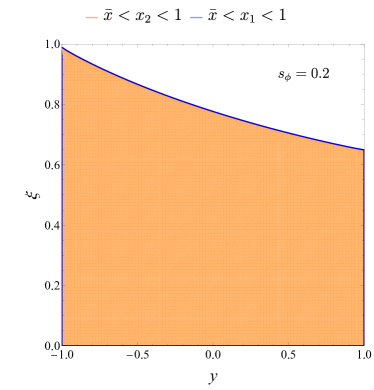
Figure 24: Physical regions in the $(y,\xi)$ radiation plane at fixed underlying Born configuration, given by $S=1876\,{\rm GeV}^{2},\bar{x}=0.01,Q^{2}=10\,{\rm GeV}^{2}$, for $s_{\phi}=0.2$ (left panel) and $s_{\phi}=-0.9$ (right panel).

fixed underlying Born configuration given by $S=1876\,{\rm GeV}^{2},\bar{x}=0.01,Q^{2}=10\,{\rm GeV}^{2}$. The doubly-covered region occurs for negative and large $s_{\phi}$ values.

A.2.3 Jacobian for ISR mapping

We write the real phase space as

$$\mathrm{d}{\bf\Phi}_{R}=\mathrm{d}x\frac{\mathrm{d}^{4}{l^{\prime}}}{(2\pi)^{3}}\delta\left({{l^{\prime}}^{2}-m_{\ell^{\prime}}^{2}}\right)\frac{\mathrm{d}^{4}k}{(2\pi)^{3}}\delta(k^{2})2\pi\delta(v^{2}-m_{v}^{2}),\quad v=xP+l-{l^{\prime}}-k.$$ (63)

Adopting FKS variables for $k$, we have

$$\frac{\mathrm{d}^{4}k}{(2\pi)^{3}}\delta(k^{2})=\frac{s}{(4\pi)^{3}}\xi\mathrm{d}\xi\mathrm{d}y\mathrm{d}\phi.$$ (64)

We perform the integration over $x$ by solving the $\delta(v^{2}-m_{v}^{2})$. To this end, taking into account eq. (41) and eq. (53), we write

$$\delta(v^{2}-m_{v}^{2})=\delta\left(\frac{1}{2}({a_{x}}x+{b_{x}}\sqrt{x}+{c_{x}})\right)=2\delta\left({a_{x}}x+{b_{x}}\sqrt{x}+{c_{x}}\right).$$ (65)

The Jacobian from the $x$ integration is given by

$$J_{x}=\int\mathrm{d}x2\delta\left({a_{x}}x+{b_{x}}\sqrt{x}+{c_{x}}\right) = \int 4y\mathrm{d}y\frac{1}{|{a_{x}}|}\delta\left((y-\sqrt{x_{1}})(y-\sqrt{x_{2}})\right)$$ (66)

$$= \int 4y\mathrm{d}y\frac{1}{|{a_{x}}|}\delta\left((y-\sqrt{x_{1}})(y-\sqrt{x_{2}})\right)$$

$$= \int 4y\mathrm{d}y\frac{1}{|{a_{x}}|}\frac{1}{|\sqrt{x_{1}}-\sqrt{x_{2}}|}\left[\delta(y-\sqrt{x_{1}})+\delta(y-\sqrt{x_{2}})\right]$$

$$= \frac{4\sqrt{x_{1,2}}}{\sqrt{\Delta_{x}}}$$

where we have performed the change of variable $y=\sqrt{x}$, and the numerator $\sqrt{x_{1,2}}$ must be chosen according to the physical solutions.

Finally, we get

$$\mathrm{d}{\bf\Phi}_{R} = J_{x}\frac{s}{(4\pi)^{3}}\xi\mathrm{d}\xi\mathrm{d}y\mathrm{d}\phi\;2\nu\times\frac{1}{2\nu}\frac{\mathrm{d}^{4}{l^{\prime}}}{(2\pi)^{2}}\delta\left({{l^{\prime}}^{2}-m_{\ell^{\prime}}^{2}}\right)$$ (67)

$$= 2\nu J_{x}\frac{s}{(4\pi)^{3}}\xi\mathrm{d}\xi\mathrm{d}y\mathrm{d}\phi\times\mathrm{d}{\bf\bar{\Phi}}_{B}\equiv J(\xi,y,\phi)\mathrm{d}\xi\mathrm{d}y\mathrm{d}\phi\times\mathrm{d}{\bf\bar{\Phi}}_{B}$$

where $\mathrm{d}{\bf\bar{\Phi}}_{B}$ is the phase space element of the underlying Born. The Jacobian associated to the radiation variable is then

$$J(\xi,y,\phi)=\frac{\nu s}{(2\pi)^{3}}\xi\sqrt{\frac{x_{1,2}}{\Delta_{x}}}.$$ (68)

A.2.4 Generation of ISR radiation

In the following, we highlight the main complications occurring at the generation stage, when the events are generated according to the POWHEG method. First, we recall that the hard scale $K_{T}(\mathbf{\Phi})_{R}$ for initial-state radiation is by default chosen to be the transverse momentum of the radiated parton $k_{T}^{2}$. For the original ISR mapping implemented in the POWHEG-BOX, $k_{T}^{2}$ assumes a relatively simple form in terms of the radiation variables $\xi,y,\phi$, i.e.

$$k_{T}^{2}=\frac{s}{4}\xi^{2}(1-y^{2})=\frac{\bar{s}}{4(1-\xi)}\xi^{2}(1-y^{2})$$ (69)

where $s$ and $\bar{s}$ are the partonic centre-of-mass energies in the real and the underlying Born configuration, respectively. While eq. (69) holds also for the case of the DIS mapping that preserves the invariant mass of the Born system (discussed in section A.2.1), the situation is more involved for the new DIS mapping preserving the lepton momenta derived in the previous section. Now the relation between $s$ and $\bar{s}$ involves the real momentum fraction $x=x(\xi,y,\phi)$, which is a complicated function of the radiation variables:

$$k_{T}^{2}=\frac{s}{4}\xi^{2}(1-y^{2})=\frac{x(\xi,y,\phi)\bar{s}}{4\bar{x}}\xi^{2}(1-y^{2}).$$ (70)

The construction for the generation of initial-state radiation in POWHEG is based on the appendix of ref. Nason:2006hfa , which in turn relies on the particular expression of $k_{T}^{2}$ in the right hand side of eq. (69). Therefore, the standard implementation provided by the POWHEG-BOX is inconsistent with the new DIS mapping. On the other hand, one can choose the POWHEG hard scale in a different way as long as it reduces to the transverse momentum of the radiated parton in the relevant soft and/or collinear limits. We exploit this freedom and define the hard scale as (in our convention the collinear singularity is approached only for $y\to-1$):

$$K_{T}^{2}(\mathbf{\Phi}_{R})=\frac{\bar{s}}{2}\xi^{2}\frac{1+y}{1+\xi y}$$ (71)

and we use as upper bound function for the veto method

$$U_{b}=\frac{N\alpha_{s}(k_{T})}{\xi(1+y)}.$$ (72)

The integration of the upper bound (including the lowest-order running for $\alpha_{s}$) times the factor $\theta(t-k_{T})$ is straightforward and the veto technique is used to generate the hardest radiation according to the POWHEG formula in eq. (4). We point out that we have chosen to use the hard scale in eq. (71) and the upper bound function in eq. (72) also for the mapping preserving the invariant mass of the Born system and the momentum of the initial lepton. Differences among various options for the hard scale are known to have impact on the resummed results only at higher orders.

A second problem is associated with the region where the DIS mapping is not invertible, i.e. in the region where there are two physical real configurations associated with the same underlying Born $\bar{\mathbf{\Phi}}_{B}$ and set of radiation variables $\xi,y,\phi$. We notice that the problematic region does not encompass any of the singular limits. Therefore, it can be removed from the real contributions that appear in the POWHEG formula and can be treated separately exploiting the standard remnant mechanism provided by the POWHEG-BOX.

A.2.5 DIS momentum mapping preserving the lepton kinematics: the FSR case

We consider now the case of a final-state singular region and we focus on a mapping that preserves the lepton kinematics. We observe that this mapping is actually the same as the one described in Sec. A.2.2 for the initial-state case. Nonetheless the meaning of the FKS radiation variables is different in the two cases and thus a dedicated construction is needed. In this section, we must assume that the final-state emitter quark is massless, since in POWHEG no mapping is associated to massive quarks. We instead retain the possibility of having a massive outgoing lepton.

The construction proceeds as follows. We work in the partonic CM frame and, as first step, we integrate out the quark momentum by exploiting the 3-momentum conservation. We adopt a parametrisation of the momenta in terms of spherical coordinates

$$\mathrm{d}\mathbf{\Phi}_{R} = \mathrm{d}x\frac{\mathrm{d}^{3}{l^{\prime}}}{(2\pi)^{3}2{l^{\prime}}^{0}}\frac{\mathrm{d}^{3}v}{(2\pi)^{3}2v^{0}}\frac{\mathrm{d}^{3}k}{(2\pi)^{3}2k^{0}}(2\pi)^{4}\delta^{4}(l+xP-{l^{\prime}}-v-k)$$ (73)

$$= \mathrm{d}x\frac{1}{8(2\pi)^{5}}\frac{\mathrm{d}^{3}{\underline{l}^{\prime}}\mathrm{d}^{3}k}{{l^{\prime}}^{0}v^{0}k^{0}}\delta\left(\sqrt{s}-{l^{\prime}}^{0}-v^{0}-k^{0}\right)$$

$$= \mathrm{d}x\frac{1}{8(2\pi)^{5}}\frac{{\underline{l}^{\prime}}^{2}\mathrm{d}{\underline{l}^{\prime}}\mathrm{d}\cos\theta_{l^{\prime}}\mathrm{d}\phi_{l^{\prime}}}{{l^{\prime}}^{0}v^{0}}k^{0}\mathrm{d}k^{0}\mathrm{d}c_{\psi}\mathrm{d}\phi$$

$$\times\delta\left(\sqrt{s}-{l^{\prime}}^{0}-\sqrt{{\underline{l}^{\prime}}^{2}+(k^{0})^{2}-2{\underline{l}^{\prime}}k^{0}c_{\psi}}-k^{0}\right),$$

where ${\underline{l}^{\prime}}$ denotes the modulus of the tri-momentum of ${l^{\prime}}$ and $c_{\psi}\equiv\cos\psi$. We use, as reference axes for the angles $\theta_{{l^{\prime}}}$ and $\psi$, the direction of the incoming lepton and that opposite to the outgoing one, respectively. We notice that we cannot use directly the direction of the outgoing quark as it has been integrated out.

We parametrise the lepton variables in terms of the DIS invariants

$$Q^{2} = \sqrt{s}({l^{\prime}}^{0}-{\underline{l}^{\prime}}\cos\theta_{{l^{\prime}}})-m_{{\ell^{\prime}}}^{2}\,,$$ (74)

$${y_{\rm dis}} = 1-\frac{{l^{\prime}}^{0}+{\underline{l}^{\prime}}\cos\theta_{{l^{\prime}}}}{\sqrt{s}}\,.$$ (75)

This is convenient in order to make transparent the connection to a Born configuration, obtained by absorbing the recoil of the radiation. In particular, the CM energy is not preserved and it changes from $s$ to $s_{b}=\lambda s$, going from a real to a Born configuration, and the partonic Born CM frame does not coincide with the real CM one, as it is the case in the standard final-state FKS mapping. The advantage of using DIS invariants rests on the fact that those variables are frame independent.

Computing the jacobian associated to the above 2-dimensional change of variables, we get

$$\operatorname{jacobian}^{-1} = \left|\frac{\partial(Q^{2},{y_{\rm dis}})}{\partial({\underline{l}^{\prime}},\cos\theta_{l^{\prime}})}\left|=\left|\begin{array}[]{ll}\sqrt{s}\left(\frac{{\underline{l}^{\prime}}}{{l^{\prime}}^{0}}-\cos\theta_{l^{\prime}}\right)&-\frac{1}{\sqrt{s}}\left(\frac{{\underline{l}^{\prime}}}{{l^{\prime}}^{0}}+\cos\theta_{l^{\prime}}\right)\\ -\sqrt{s}{\underline{l}^{\prime}}&-\frac{1}{\sqrt{s}}{\underline{l}^{\prime}}\end{array}\right|=2\frac{{\underline{l}^{\prime}}^{2}}{{l^{\prime}}^{0}}\,.\right.\right.$$ (78)

Then, we get

$$\mathrm{d}\mathbf{\Phi}_{R}=\mathrm{d}x\frac{1}{16(2\pi)^{5}}\frac{\mathrm{d}Q^{2}\mathrm{d}{y_{\rm dis}}\mathrm{d}\phi_{l^{\prime}}}{v^{0}}k^{0}\mathrm{d}k^{0}\mathrm{d}c_{\psi}\mathrm{d}\phi\delta\left(\sqrt{s}-{l^{\prime}}^{0}-v^{0}-k^{0}\right).$$ (79)

In order to make contact with the FKS parametrisation, we want to pass from $c_{\psi}$ to the FKS variable $y$, that is the cosine of the angle between $l^{\prime}$ and $v$. Using Carnot’s formula, we have

$$y=\frac{{\underline{l}^{\prime}}^{2}-v_{0}^{2}-(k^{0})^{2}}{2v^{0}k^{0}}=\frac{2c_{\psi}{\underline{l}^{\prime}}-\sqrt{s}\xi}{\sqrt{4{\underline{l}^{\prime}}^{2}-4c_{\psi}{\underline{l}^{\prime}}\sqrt{s}\xi+s\xi^{2}}},$$ (80)

with $v^{0}=\sqrt{{\underline{l}^{\prime}}^{2}+(k^{0})^{2}-2c_{\psi}{\underline{l}^{\prime}}k^{0}}$. The derivative with respect to $c_{\psi}$

$$\frac{\mathrm{d}y}{\mathrm{d}c_{\psi}}=\frac{{4{\underline{l}^{\prime}}}^{2}}{\left(4{\underline{l}^{\prime}}^{2}-4c_{\psi}{\underline{l}^{\prime}}\sqrt{s}\xi+s\xi^{2}\right)^{3/2}}\left(2{\underline{l}^{\prime}}-c_{\psi}\sqrt{s}\xi\right),$$ (81)

is positive for ${\underline{l}^{\prime}}>k^{0}$. In this case, $y$ is a monotonically increasing function of $c_{\psi}$ and admits an unique inverse. The inverse can be obtained by taking the square and solving the resulting quadratic equation for $c_{\psi}$

$$y^{2} = \frac{\left(2c_{\psi}{\underline{l}^{\prime}}-\sqrt{s}\xi\right)^{2}}{4{\underline{l}^{\prime}}^{2}-4c_{\psi}{\underline{l}^{\prime}}\sqrt{s}\xi+s\xi^{2}},$$

$$\implies c_{\psi} = \frac{\pm y\sqrt{4{\underline{l}^{\prime}}^{2}-s\xi^{2}(1-y^{2})}+\sqrt{s}\xi(1-y^{2})}{2{\underline{l}^{\prime}}}.$$ (82)

For ${\underline{l}^{\prime}}>k^{0}$, we must take the upper sign, that guarantees that $c_{\psi}$ is a monotonically increasing function of $y$ mapping the $[-1,1]$ interval biunivocally into itself. For ${\underline{l}^{\prime}}<k^{0}$ both signs are acceptable. The possible cases are depicted in figure 25, where we exploit the geometrical relation among the angles $c_{\psi}$ and $y=\cos(\pi-\theta_{y})=-\cos(\theta_{y})$ and the lengths $v^{0}$, $k^{0}$ and ${\underline{l}^{\prime}}$ forming a triangle. The left panel corresponds to the case ${\underline{l}^{\prime}}>k^{0}$. It is clear that there is a one-to-one correspondence between $c_{\psi}$ and $y$.

On the other hand, for the case $k^{0}>{\underline{l}^{\prime}}$ shown in the right panel, the range of $\theta_{y}$ corresponding to $c_{\psi}\in[-1,1]$ does not fully cover the interval $[0,\pi]$ and in particular $\theta_{y}$ goes from 0 up to a maximum value strictly lower than $\pi$ such that the collinear region is excluded. Furthermore, because the transverse momentum of the two final state partons has to compensate the one of the lepton, radiation has to be necessarily in the anticollinear region, at $y<0$.

Figure 25: Geometric illustration of the relation between the angle $\psi$ and the standard FKS one $\pi-\theta_{y}$ for the two cases ${\underline{l}^{\prime}}>k^{0}$ (left) and ${\underline{l}^{\prime}}<k^{0}$ (right).

This region can be covered by the remnant mechanism, since it is not singular. Correspondingly, for ${\underline{l}^{\prime}}<k^{0}$, we must have $y<0$ and

$$v^{0}=\frac{1}{2}\left(\pm\sqrt{4{\underline{l}^{\prime}}^{2}-s\xi^{2}(1-y^{2})}-\sqrt{s}\xi y\right),$$ (83)

while for ${\underline{l}^{\prime}}>k^{0}$, we have

$$v^{0}=\frac{1}{2}\left(\sqrt{4{\underline{l}^{\prime}}^{2}-s\xi^{2}(1-y^{2})}-\sqrt{s}\xi y\right).$$ (84)

The choice of the sign guarantees that for $y=-1$

$$v^{0}=\frac{1}{2}\left(2{\underline{l}^{\prime}}+\sqrt{s}\xi\right)={\underline{l}^{\prime}}+k^{0}\,,$$ (85)

and for $y=1$

$$v^{0}=\frac{1}{2}\left(2{\underline{l}^{\prime}}-\sqrt{s}\xi\right)={\underline{l}^{\prime}}-k^{0}\,.$$ (86)

Using the relation 82 we can compute the jacobian factor associated with the change of variable $c_{\psi}\to y$, and we get

$$J_{y}=\left|\frac{4\sqrt{s}\xi yv^{0}-(4{\underline{l}^{\prime}}^{2}-s\xi^{2})}{2{\underline{l}^{\prime}}\sqrt{4{\underline{l}^{\prime}}^{2}-s\xi^{2}(1-y^{2})}}\right|=\frac{(v^{0})^{2}}{{\underline{l}^{\prime}}|v^{0}+k^{0}y|}\,,$$ (87)

where we have conveniently identified a factor $v_{0}$ to simplify the notation. Then, we have

$$\mathrm{d}\mathbf{\Phi}_{R}=\mathrm{d}x\frac{1}{16(2\pi)^{5}}\frac{\mathrm{d}Q^{2}\mathrm{d}{y_{\rm dis}}\mathrm{d}\phi_{l^{\prime}}}{v^{0}}k^{0}\mathrm{d}k^{0}\mathrm{d}y\mathrm{d}\phi\,J_{y}\delta\left(\sqrt{s}-{l^{\prime}}^{0}-v^{0}-k^{0}\right).$$ (88)

The last step in the construction of the full jacobian factor is to perform the change of variable $x=s/S$ and integrate in $\mathrm{d}s$ exploiting the $\delta$ function. As a result, the $\delta$ function enforces the relation

$$s=\frac{2Q^{2}-(Q^{2}+m_{{\ell^{\prime}}}^{2})\xi(1-y)}{{y_{\rm dis}}(2-\xi(1-y))-\xi(1-\xi)(1-y)}$$ (89)

and after using the properties of the Dirac $\delta$ and a bit of algebra we have the last jacobian factor

$$J_{\delta}=\left|\frac{4\sqrt{s}\left(2s-2\sqrt{s}l^{0}-s\xi(1-y)\right)/s}{(4+2(\xi^{2}-2\xi)(1-y)-2(1-{y_{\rm dis}})(2-\xi(1-y)))}\right|=\frac{4|v^{0}+k^{0}y|}{2{y_{\rm dis}}-\xi(1+{y_{\rm dis}}-\xi)(1-y)}$$ (90)

so that the final expression reads

$$\mathrm{d}\mathbf{\Phi}_{R} = \frac{1}{S}\frac{1}{16(2\pi)^{5}}\frac{\mathrm{d}Q^{2}\mathrm{d}{y_{\rm dis}}\mathrm{d}\phi_{{l^{\prime}}}}{v^{0}}k^{0}\mathrm{d}k^{0}\mathrm{d}y\mathrm{d}\phi J_{y}J_{\delta}$$ (91)

$$= \frac{1}{S}\frac{1}{4(2\pi)^{5}}\frac{k^{0}v^{0}\mathrm{d}Q^{2}\mathrm{d}{y_{\rm dis}}\mathrm{d}\phi_{{l^{\prime}}}\mathrm{d}k^{0}\mathrm{d}y\mathrm{d}\phi}{{\underline{l}^{\prime}}(2{y_{\rm dis}}-\xi(1+{y_{\rm dis}}-\xi)(1-y))}$$ (92)

$$= \frac{{y_{\rm dis}}}{2{y_{\rm dis}}-\xi(1+{y_{\rm dis}}-\xi)(1-y)}\frac{2v^{0}}{{\underline{l}^{\prime}}}\frac{\mathrm{d}^{3}k}{(2\pi)^{3}2k^{0}}\times\mathrm{d}\mathbf{\bar{\Phi}}_{B}$$ (93)

A.2.6 Generation of FSR radiation

Being the map among real and born configuration essentially the same for FSR and ISR, similar considerations apply for the definition of the hard scale for FSR. The original choice done in the POWHEG-BOX framework are slightly modified to consistently address the case of DIS. We use as evolution variable

$$K_{T}^{2}(\mathbf{\Phi}_{R})=\frac{\bar{s}}{2}\xi^{2}(1-y)\,,$$ (94)

and as upper bound function

$$U_{b}=\frac{N\alpha_{s}(k_{T})}{\xi(1-y)}\,.$$ (95)

Note that for the case of final state radiation in our mapping the collinear region is approached in the limit $y\to 1$, and the upper bound function is the same as for the case of initial state radiation.

Appendix B Further NLO validation plots

For convenience we show here our validation plots for other relevant cases of lepton-hadron DIS processes. The setup, cuts and scale setting are the same as reported in section 2.1.

Figure 26: Same as figure 3 for charged current $\nu_{\tau}$ ($\bar{\nu}_{\tau}$) DIS with $m_{\tau}=1.777\,$GeV and charm quark production setting $m_{c}=1.5\,$GeV.

Figure 27: Same as figure 3 for charged current $l^{-}$ ($l^{+}$) DIS.

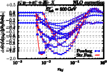
Figure 28: Same as figure 3 for NC $\nu_{e}$ ($\bar{\nu}_{e}$) DIS.

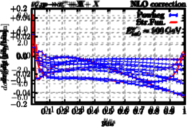
Figure 29: Same as figure 3 for NC $l^{-}$ ($l^{+}$) DIS.

References

- (1) G. Miller, E. D. Bloom, G. Buschhorn, D. H. Coward, H. DeStaebler, J. Drees et al., Inelastic electron-proton scattering at large momentum transfers and the inelastic structure functions of the proton, Phys. Rev. D 5 (Feb, 1972) 528–544.
- (2) Gargamelle Neutrino collaboration, F. J. Hasert et al., Observation of Neutrino Like Interactions Without Muon Or Electron in the Gargamelle Neutrino Experiment, Phys. Lett. B 46 (1973) 138–140.
- (3) FASER collaboration, H. Abreu et al., First Direct Observation of Collider Neutrinos with FASER at the LHC, Phys. Rev. Lett. 131 (2023) 031801, [2303.14185].
- (4) SND@LHC collaboration, R. Albanese et al., Observation of Collider Muon Neutrinos with the SND@LHC Experiment, Phys. Rev. Lett. 131 (2023) 031802, [2305.09383].
- (5) OPERA collaboration, N. Agafonova et al., Final Results of the OPERA Experiment on Appearance in the CNGS Neutrino Beam, Phys. Rev. Lett. 120 (2018) 211801, [1804.04912].
- (6) DONuT collaboration, K. Kodama et al., Final tau-neutrino results from the DONuT experiment, Phys. Rev. D 78 (2008) 052002, [0711.0728].
- (7) M. H. Reno, High-Energy to Ultrahigh-Energy Neutrino Interactions, Ann. Rev. Nucl. Part. Sci. 73 (2023) 181–204.
- (8) SHiP collaboration, M. Anelli et al., A facility to Search for Hidden Particles (SHiP) at the CERN SPS, 1504.04956.
- (9) R. Abdul Khalek et al., Science Requirements and Detector Concepts for the Electron-Ion Collider: EIC Yellow Report, Nucl. Phys. A 1026 (2022) 122447, [2103.05419].
- (10) C. H. Albright and C. Jarlskog, Neutrino Production of m+ and e+ Heavy Leptons. 1., Nucl. Phys. B 84 (1975) 467–492.
- (11) S. Kretzer and M. H. Reno, Tau neutrino deep inelastic charged current interactions, Phys. Rev. D 66 (2002) 113007, [hep-ph/0208187].
- (12) H. Liu, A. Rashed and A. Datta, Probing lepton nonuniversality in tau neutrino scattering, Phys. Rev. D 92 (2015) 073016, [1505.04594].
- (13) S. Alekhin et al., A facility to Search for Hidden Particles at the CERN SPS: the SHiP physics case, Rept. Prog. Phys. 79 (2016) 124201, [1504.04855].
- (14) ATLAS collaboration, M. Aaboud et al., Measurement of the -boson mass in pp collisions at TeV with the ATLAS detector, Eur. Phys. J. C 78 (2018) 110, [1701.07240].
- (15) S. Moch, J. A. M. Vermaseren and A. Vogt, The Longitudinal structure function at the third order, Phys. Lett. B 606 (2005) 123–129, [hep-ph/0411112].
- (16) J. A. M. Vermaseren, A. Vogt and S. Moch, The Third-order QCD corrections to deep-inelastic scattering by photon exchange, Nucl. Phys. B 724 (2005) 3–182, [hep-ph/0504242].
- (17) S. Moch, J. A. M. Vermaseren and A. Vogt, Third-order QCD corrections to the charged-current structure function F(3), Nucl. Phys. B 813 (2009) 220–258, [0812.4168].
- (18) J. Davies, A. Vogt, S. Moch and J. A. M. Vermaseren, Non-singlet coefficient functions for charged-current deep-inelastic scattering to the third order in QCD, PoS DIS2016 (2016) 059, [1606.08907].
- (19) J. Blümlein, P. Marquard, C. Schneider and K. Schönwald, The massless three-loop Wilson coefficients for the deep-inelastic structure functions F2, FL, xF3 and g1, JHEP 11 (2022) 156, [2208.14325].
- (20) J. Currie, T. Gehrmann, E. W. N. Glover, A. Huss, J. Niehues and A. Vogt, N3LO corrections to jet production in deep inelastic scattering using the Projection-to-Born method, JHEP 05 (2018) 209, [1803.09973].
- (21) T. Gehrmann, A. Huss, J. Niehues, A. Vogt and D. M. Walker, Jet production in charged-current deep-inelastic scattering to third order in QCD, Phys. Lett. B 792 (2019) 182–186, [1812.06104].
- (22) I. Borsa, D. de Florian and I. Pedron, NNLO jet production in neutral and charged current polarized deep inelastic scattering, Phys. Rev. D 107 (2023) 054027, [2212.06625].
- (23) T. Gottschalk, Chromodynamic Corrections to Neutrino Production of Heavy Quarks, Phys. Rev. D 23 (1981) 56.
- (24) M. Gluck, S. Kretzer and E. Reya, The Strange sea density and charm production in deep inelastic charged current processes, Phys. Lett. B 380 (1996) 171–176, [hep-ph/9603304].
- (25) M. Buza, Y. Matiounine, J. Smith and W. L. van Neerven, Charm electroproduction viewed in the variable flavor number scheme versus fixed order perturbation theory, Eur. Phys. J. C 1 (1998) 301–320, [hep-ph/9612398].
- (26) J. Blümlein, A. Hasselhuhn and T. Pfoh, The heavy quark corrections to charged current deep-inelastic scattering at large virtualities, Nucl. Phys. B 881 (2014) 1–41, [1401.4352].
- (27) E. L. Berger, J. Gao, C. S. Li, Z. L. Liu and H. X. Zhu, Charm-Quark Production in Deep-Inelastic Neutrino Scattering at Next-to-Next-to-Leading Order in QCD, Phys. Rev. Lett. 116 (2016) 212002, [1601.05430].
- (28) M. Bahr et al., Herwig++ Physics and Manual, Eur. Phys. J. C 58 (2008) 639–707, [0803.0883].
- (29) J. Bellm et al., Herwig 7.2 release note, Eur. Phys. J. C 80 (2020) 452, [1912.06509].
- (30) T. Gleisberg, S. Hoeche, F. Krauss, M. Schonherr, S. Schumann, F. Siegert et al., Event generation with SHERPA 1.1, JHEP 02 (2009) 007, [0811.4622].
- (31) Sherpa collaboration, E. Bothmann et al., Event Generation with Sherpa 2.2, SciPost Phys. 7 (2019) 034, [1905.09127].
- (32) T. Sjöstrand, S. Ask, J. R. Christiansen, R. Corke, N. Desai, P. Ilten et al., An introduction to PYTHIA 8.2, Comput. Phys. Commun. 191 (2015) 159–177, [1410.3012].
- (33) T. Carli, T. Gehrmann and S. Hoeche, Hadronic final states in deep-inelastic scattering with Sherpa, Eur. Phys. J. C 67 (2010) 73–97, [0912.3715].
- (34) A. Banfi, S. Ferrario Ravasio, B. Jäger, A. Karlberg, F. Reichenbach and G. Zanderighi, A POWHEG generator for deep inelastic scattering, JHEP 02 (2024) 023, [2309.02127].
- (35) I. Borsa and B. Jäger, Parton-shower effects in polarized deep inelastic scattering, 2404.07702.
- (36) S. Höche, S. Kuttimalai and Y. Li, Hadronic Final States in DIS at NNLO QCD with Parton Showers, Phys. Rev. D 98 (2018) 114013, [1809.04192].
- (37) C. Andreopoulos et al., The GENIE Neutrino Monte Carlo Generator, Nucl. Instrum. Meth. A 614 (2010) 87–104, [0905.2517].
- (38) A. Garcia, R. Gauld, A. Heijboer and J. Rojo, Complete predictions for high-energy neutrino propagation in matter, JCAP 09 (2020) 025, [2004.04756].
- (39) P. Nason, A New method for combining NLO QCD with shower Monte Carlo algorithms, JHEP 11 (2004) 040, [hep-ph/0409146].
- (40) S. Frixione, P. Nason and C. Oleari, Matching NLO QCD computations with Parton Shower simulations: the POWHEG method, JHEP 11 (2007) 070, [0709.2092].
- (41) S. Alioli, P. Nason, C. Oleari and E. Re, A general framework for implementing NLO calculations in shower Monte Carlo programs: the POWHEG BOX, JHEP 06 (2010) 043, [1002.2581].
- (42) GoSam collaboration, G. Cullen et al., GS-2.0: a tool for automated one-loop calculations within the Standard Model and beyond, Eur. Phys. J. C 74 (2014) 3001, [1404.7096].
- (43) S. Frixione, Z. Kunszt and A. Signer, Three jet cross-sections to next-to-leading order, Nucl. Phys. B 467 (1996) 399–442, [hep-ph/9512328].
- (44) S. Catani and M. H. Seymour, A General algorithm for calculating jet cross-sections in NLO QCD, Nucl. Phys. B 485 (1997) 291–419, [hep-ph/9605323].
- (45) W. Furmanski and R. Petronzio, Lepton - Hadron Processes Beyond Leading Order in Quantum Chromodynamics, Z. Phys. C 11 (1982) 293.
- (46) NNPDF collaboration, R. D. Ball et al., Parton distributions from high-precision collider data, Eur. Phys. J. C 77 (2017) 663, [1706.00428].
- (47) A. Buckley, J. Ferrando, S. Lloyd, K. Nordström, B. Page, M. Rüfenacht et al., LHAPDF6: parton density access in the LHC precision era, Eur. Phys. J. C 75 (2015) 132, [1412.7420].
- (48) L. Buonocore, P. Nason and F. Tramontano, Heavy quark radiation in NLO+PS POWHEG generators, Eur. Phys. J. C 78 (2018) 151, [1711.06281].
- (49) L. Barze, G. Montagna, P. Nason, O. Nicrosini and F. Piccinini, Implementation of electroweak corrections in the POWHEG BOX: single W production, JHEP 04 (2012) 037, [1202.0465].
- (50) M. Cacciari, M. Greco and P. Nason, The spectrum in heavy-flavour hadroproduction., JHEP 05 (1998) 007, [hep-ph/9803400].
- (51) M. Cacciari, G. P. Salam and G. Soyez, The anti- jet clustering algorithm, JHEP 04 (2008) 063, [0802.1189].
- (52) M. Cacciari, G. P. Salam and G. Soyez, FastJet User Manual, Eur. Phys. J. C 72 (2012) 1896, [1111.6097].
- (53) G. P. Salam and J. Rojo, A Higher Order Perturbative Parton Evolution Toolkit (HOPPET), Comput. Phys. Commun. 180 (2009) 120–156, [0804.3755].
- (54) A. Karlberg, P. Nason, G. Salam, G. Zanderighi and F. Dreyer, “Hoppet v1.3.0 release note.”.
- (55) J. Gao, Massive charged-current coefficient functions in deep-inelastic scattering at NNLO and impact on strange-quark distributions, JHEP 02 (2018) 026, [1710.04258].
- (56) A. Candido, F. Hekhorn, G. Magni, T. R. Rabemananjara and R. Stegeman, Yadism: Yet Another Deep-Inelastic Scattering Module, 2401.15187.
- (57) ZEUS collaboration, I. Abt et al., Charm production in charged current deep inelastic scattering at HERA, JHEP 05 (2019) 201, [1904.03261].
- (58) M. Arratia, Y. Furletova, T. J. Hobbs, F. Olness and S. J. Sekula, Charm jets as a probe for strangeness at the future Electron-Ion Collider, Phys. Rev. D 103 (2021) 074023, [2006.12520].
- (59) ZEUS collaboration, S. Chekanov et al., Forward jet production in deep inelastic ep scattering and low-x parton dynamics at HERA, Phys. Lett. B 632 (2006) 13–26, [hep-ex/0502029].
- (60) M. Cacciari, F. A. Dreyer, A. Karlberg, G. P. Salam and G. Zanderighi, Fully Differential Vector-Boson-Fusion Higgs Production at Next-to-Next-to-Leading Order, Phys. Rev. Lett. 115 (2015) 082002, [1506.02660].
- (61) S. Alekhin, J. Blumlein and S. Moch, Parton Distribution Functions and Benchmark Cross Sections at NNLO, Phys. Rev. D 86 (2012) 054009, [1202.2281].
- (62) I. Bierenbaum, J. Blumlein and S. Klein, The Gluonic Operator Matrix Elements at O(alpha(s)**2) for DIS Heavy Flavor Production, Phys. Lett. B 672 (2009) 401–406, [0901.0669].
- (63) SND@LHC collaboration, G. Acampora et al., SND@LHC: the scattering and neutrino detector at the LHC, JINST 19 (2024) P05067, [2210.02784].
- (64) L. Buonocore, F. Kling, L. Rottoli and J. Sominka, Predictions for neutrinos and new physics from forward heavy hadron production at the LHC, Eur. Phys. J. C 84 (2024) 363, [2309.12793].
- (65) FASER collaboration, R. Mammen Abraham et al., Neutrino Rate Predictions for FASER, 2402.13318.
- (66) IceCube collaboration, M. G. Aartsen et al., Measurement of Atmospheric Tau Neutrino Appearance with IceCube DeepCore, Phys. Rev. D 99 (2019) 032007, [1901.05366].
- (67) A. Cooper-Sarkar, P. Mertsch and S. Sarkar, The high energy neutrino cross-section in the Standard Model and its uncertainty, JHEP 08 (2011) 042, [1106.3723].
- (68) K. Hamilton, P. Nason, C. Oleari and G. Zanderighi, Merging H/W/Z + 0 and 1 jet at NLO with no merging scale: a path to parton shower + NNLO matching, JHEP 05 (2013) 082, [1212.4504].
- (69) K. Hamilton, P. Nason, E. Re and G. Zanderighi, NNLOPS simulation of Higgs boson production, JHEP 10 (2013) 222, [1309.0017].
- (70) P. F. Monni, P. Nason, E. Re, M. Wiesemann and G. Zanderighi, MiNNLOPS: a new method to match NNLO QCD to parton showers, JHEP 05 (2020) 143, [1908.06987].
- (71) P. Nason and G. Ridolfi, A Positive-weight next-to-leading-order Monte Carlo for Z pair hadroproduction, JHEP 08 (2006) 077, [hep-ph/0606275].