Progressive Entropic Optimal Transport Solvers

Abstract

Optimal transport (OT) has profoundly impacted machine learning by providing theoretical and computational tools to realign datasets. In this context, given two large point clouds of sizes $n$ and $m$ in $\mathbb{R}^{d}$, entropic OT (EOT) solvers have emerged as the most reliable tool to either solve the Kantorovitch problem and output a $n\times m$ coupling matrix, or to solve the Monge problem and learn a vector-valued push-forward map. While the robustness of EOT couplings/maps makes them a go-to choice in practical applications, EOT solvers remain difficult to tune because of a small but influential set of hyperparameters, notably the omnipresent entropic regularization strength $\varepsilon$. Setting $\varepsilon$ can be difficult, as it simultaneously impacts various performance metrics, such as compute speed, statistical performance, generalization, and bias. In this work, we propose a new class of EOT solvers (ProgOT), that can estimate both plans and transport maps. We take advantage of several opportunities to optimize the computation of EOT solutions by dividing mass displacement using a time discretization, borrowing inspiration from dynamic OT formulations (McCann, 1997), and conquering each of these steps using EOT with properly scheduled parameters. We provide experimental evidence demonstrating that ProgOT is a faster and more robust alternative to EOT solvers when computing couplings and maps at large scales, even outperforming neural network-based approaches. We also prove the statistical consistency of ProgOT when estimating OT maps.

1 Introduction

Many problems in generative machine learning and natural sciences—notably biology (Schiebinger et al., 2019; Bunne et al., 2023), astronomy (Métivier et al., 2016) or quantum chemistry (Buttazzo et al., 2012)—require aligning datasets or learning to map data points from a source to a target distribution. These problems stand at the core of optimal transport theory (Santambrogio, 2015) and have spurred the proposal of various solvers (Peyré et al., 2019) to perform these tasks reliably. In these tasks, we are given $n$ and $m$ points respectively sampled from source and target probability distributions on $\mathbb{R}^{d}$, with the goal of either returning a coupling matrix of size $n\times m$ (which solves the so-called Kantorovitch problem), or a vector-valued map estimator that extends to out-of-sample data (solving the Monge problem).

In modern applications, where $n,m\gtrsim 10^{4}$, a popular approach to estimating either coupling or maps is to rely on a regularization of the original Kantorovitch linear OT formulation using neg-entropy. This technique, referred to as entropic OT, can be traced back to Schrödinger and was popularized for ML applications in (Cuturi, 2013) (see Section 2). Crucially, EOT can be solved efficiently with Sinkhorn’s algorithm (Algorithm 1), with favorable computational (Altschuler et al., 2017; Lin et al., 2022) and statistical properties (Genevay, 2019; Mena and Niles-Weed, 2019) compared to linear programs. Most couplings computed nowadays on large point clouds within ML applications are obtained using EOT solvers that rely on variants of the Sinkhorn algorithm, whether explicitly, or as a lower-level subroutine (Scetbon et al., 2021, 2022). The widespread adoption of EOT has spurred many modifications of Sinkhorn’s original algorithm (e.g., through acceleration (Thibault et al., 2021) or initialization (Thornton and Cuturi, 2023)), and encouraged its incorporation within neural-network OT approaches (Pooladian et al., 2023; Tong et al., 2023; Uscidda and Cuturi, 2023).

Figure 1: (left) EOT solvers collapse when the value of $\varepsilon$ is not properly chosen. This typically results in biased map estimators and in blurry couplings (see Fig. 2 for the coupling matrix obtained between ${\mathbf{x}}_{\text{train}}$ and ${\mathbf{y}}_{\text{train}}$). (middle) Debiasing the output of EOT solvers can prevent a collapse to the mean seen in EOT estimators, but computes the same coupling. ProgOT (right) ameliorates these problems in various ways: by decomposing the resolution of the OT problem into multiple time steps, and using various forms of progressive scheduling, we recover both a coupling whose entropy can be tuned automatically and a map estimator that is fast and reliable.

Figure 2: Coupling matrices between train points in Fig. 1. Comparison of EOT with a fairly large $\varepsilon$, and ProgOT which automatically tunes the entropy of its coupling according to the target point cloud’s dispersion.

Though incredibly popular, Sinkhorn’s algorithm is not without its drawbacks. While a popular tool due its scalability and simplicity, its numerical behavior is deeply impacted by the amount of neg-entropy regularization, driven by the hyperparameter $\varepsilon$. Some practitioners suggest to have the parameter nearly vanish (Xie et al., 2020; Schmitzer, 2019), others consider the case where it diverges, highlighting links with the maximum mean discrepancy (Ramdas et al., 2017; Genevay et al., 2019).

Several years after its introduction to the machine learning community (Cuturi, 2013), choosing a suitable regularization term for EOT remains a thorny pain point. Common approaches are setting $\varepsilon>0$ to a default value (e.g., the max (Flamary et al., 2021) or mean (Cuturi et al., 2022b) normalization of the transport cost matrix), incorporating a form of cross-validation or an unsupervised criterion (Vacher and Vialard, 2022; Van Assel et al., 2023), or scheduling $\varepsilon$ (Lehmann et al., 2022; Feydy, 2020). When $\varepsilon$ is too large, the algorithm converges quickly, but yields severely biased maps (Figure 1, left), or blurry, uninformative couplings (Figure 2). Even theoretically and numerically debiasing the Sinkhorn solver (Figure 1, middle) does not seem to fully resolve the issue (Feydy et al., 2019; Pooladian et al., 2022). To conclude, while strategies exist to alleviate this bias, there currently exists no one-size-fits-all solution to this problem.

Our contribution: an EOT solver with a dynamic lens. Recent years have witnessed an explosion in neural-network approaches based on the so-called  Benamou and Brenier dynamic formulation of OT (Lipman et al., 2022; Liu, 2022; Tong et al., 2023; Pooladian et al., 2023). A benefit of this perspective is the ability to split the OT problem into simpler sub-problems that are likely better conditioned than the initial transport problem. With this observation, we propose a novel family of progressive EOT solvers, called ProgOT, that are meant to be sturdier and easier to parameterize than existing solvers. Our key idea is to exploit the dynamic nature of the problem, and vary parameters dynamically, such as $\varepsilon$ and convergence thresholds, along the transport. We show that ProgOT

• can be used to recover both Kantorovitch couplings and Monge map estimators,

• strikes the right balance between computational and statistical tradeoffs,

• can outperform other (including neural-network based) approaches on real datasets,

• gives rise to a novel, provably statistically consistent map estimator under standard assumptions.

2 Background

Optimal transport. For domain $\Omega\subseteq{\mathbb{R}}^{d}$, let ${\mathcal{P}}_{2}(\Omega)$ denote the space of probability measures over $\Omega$ with a finite second moment, and let ${\mathcal{P}}_{2,\text{ac}}(\Omega)$ be those with densities. Let $\mu,\nu\in{\mathcal{P}}_{2}(\Omega)$, and let $\Gamma(\mu,\nu)$ be the set of joint probability measures with left-marginal $\mu$ and right-marginal $\nu$. We consider a translation invariant cost function $c(x,y):=h(x-y)$, with $h$ a strictly convex function, and define the Wasserstein distance, parameterized by $h$, between $\mu$ and $\nu$

$$W(\mu,\nu)\coloneqq\inf_{\pi\in\Gamma(\mu,\nu)}\iint h(x-y)\mathrm{d}\pi(x,y)\,.$$ (1)

This formulation is due to Kantorovitch (1942), and we call the minimizers to (1) OT couplings or OT plans, and denote it as $\pi_{0}$. A subclass of couplings are those induced by pushforward maps. We say that $T:{\mathbb{R}}^{d}\to{\mathbb{R}}^{d}$ pushes $\mu$ forward to $\nu$ if $T(X)\sim\nu$ for $X\sim\mu$, and write $T_{\#}\mu=\nu$. Given a choice of cost, we can define the Monge (1781) formulation of OT

$$T_{0}\coloneqq\operatorname*{arg\,min}_{T:T_{\#}\mu=\nu}\int h(x-T(x))\mathrm{d}\mu(x)\,$$ (2)

where the minimizers are referred to as Monge maps, or OT maps from $\mu$ to $\nu$. Unlike OT couplings, OT maps are not always guaranteed to exist. Though, if $\mu$ has a density, we obtain significantly more structure on the OT map:

Theorem 1 (Brenier’s Theorem (1991)).

Suppose $\mu\in{\mathcal{P}}_{2,\text{ac}}(\Omega)$ and $\nu\in{\mathcal{P}}_{2}(\Omega)$. Then there exists a unique solution to (2) that is of the form $T_{0}=\operatorname{Id}-\nabla h^{*}\circ\nabla f_{0}$, where $h^{*}$ is the convex-conjugate of $h$, i.e. $h^{*}(y)\coloneqq\max_{x}\langle x,y\rangle-h(x)$, and

$$(f_{0},g_{0})\in\operatorname*{arg\,max}_{(f,g)\in{\mathcal{F}}}\int f\mathrm{d}\mu+\int g\mathrm{d}\nu\,,$$ (3)

where ${\mathcal{F}}\coloneqq\{(f,g)\in L^{1}(\mu)\times L^{1}(\nu):\ f(x)+g(y)\leq h(x-y),\,\forall x,y\in\Omega.\}$. Moreover, the OT plan is given by $\pi_{0}(\mathrm{d}x,\mathrm{d}y)=\delta_{T_{0}(x)}(y)\mu(\mathrm{d}x)$.

Importantly, (3) is the dual problem to (1) and the pair of functions $(f_{0},g_{0})$ are referred to as the optimal Kantorovich potentials. Lastly, we recall the notion of geodesics with respect to the Wasserstein distance. For a pair of measures $\mu$ and $\nu$ with OT map $T_{0}$, the McCann interpolation between $\mu$ and $\nu$ is defined as

$$\mu_{\alpha}\coloneqq((1-\alpha)\operatorname{Id}+\alpha T_{0})_{\#}\mu\,,$$ (4)

where $\alpha\in[0,1]$. Equivalently, $\mu_{\alpha}$ is the law of $X_{\alpha}=(1-\alpha)X+\alpha T_{0}(X)$, where $X\sim\mu$. In the case where $h=\|\cdot\|^{p}$ for $p>1$, the McCann interpolation is in fact a geodesic in the Wasserstein space (Ambrosio et al., 2005). While this equivalence may not hold for general costs, the McCann interpolation still provides a natural path of measures between $\mu$ and $\nu$ (Liu, 2022).

Algorithm 1 Sink$(\mathbf{a},\mathbf{X},\mathbf{b},\mathbf{Y},\varepsilon,\tau,\mathbf{f}_{\text{init}},\mathbf{g}_{\text{init}})$.

1:$\mathbf{f},\mathbf{g}\leftarrow\mathbf{f}_{\text{init}},\mathbf{g}_{\text{init}}$ (zero by default)

2:$\mathbf{x}_{1},\dots,\mathbf{x}_{n}=\mathbf{X},\quad\mathbf{y}_{1},\dots,\mathbf{y}_{m}=\mathbf{Y}$

3:$\mathbf{C}\leftarrow[h(\mathbf{x}_{i}-\mathbf{y}_{j})]_{ij}$

4:while $\|\exp\left(\tfrac{\mathbf{C}-\mathbf{f}\oplus\mathbf{g}}{\varepsilon}\right)\mathbf{1}_{m}-\mathbf{a}\|_{1}<\tau$ do

5:     $\mathbf{f}\leftarrow\varepsilon\log\mathbf{a}-\min_{\varepsilon}(\mathbf{C}-\mathbf{f}\oplus\mathbf{g})+\mathbf{f}$

6:     $\mathbf{g}\leftarrow\varepsilon\log\mathbf{b}-\min_{\varepsilon}(\mathbf{C}^{\top}-\mathbf{g}\oplus\mathbf{f})+\mathbf{g}$

7:end while

8:return $\mathbf{f},\mathbf{g},\mathbf{P}=\exp\left((\mathbf{C}-\mathbf{f}\oplus\mathbf{g})/\varepsilon\right)$

Entropic OT.

Entropic regularization has become the de-facto approach to estimate all three variables $\pi_{0}$, $f_{0}$ and $T_{0}$ using samples $(\mathbf{x}_{1},\ldots,\mathbf{x}_{n})$ and $(\mathbf{y}_{1},\ldots,\mathbf{y}_{m})$, both weighted by a probability weight vectors $\mathbf{a}\in\mathbb{R}^{n}_{+},\mathbf{b}\in\mathbb{R}^{m}_{+}$ summing to $1$, to form approximations $\hat{\mu}_{n}=\sum_{i=1}^{n}\mathbf{a}_{i}\delta_{\mathbf{x}_{i}}$ and $\hat{\nu}_{m}=\sum_{i=1}^{m}\mathbf{b}_{j}\delta_{\mathbf{y}_{j}}$. A common formulation of the EOT problem is the following $\varepsilon$-strongly concave program:

$$\mathbf{f}^{\star},\mathbf{g}^{\star}=\operatorname*{arg\,max}_{\begin{subarray}{c}\mathbf{f}\in{\mathbb{R}}^{n},\mathbf{g}\in{\mathbb{R}}^{m}\end{subarray}} \langle\mathbf{f},\mathbf{a}\rangle+\langle\mathbf{g},\mathbf{b}\rangle$$

$$-\varepsilon\langle e^{\mathbf{f}/\varepsilon},\mathbf{K}e^{\mathbf{g}/\varepsilon}\rangle\,,$$ (5)

where $\varepsilon>0$ and $\mathbf{K}_{i,j}=[\exp(-(\mathbf{x}_{i}-\mathbf{y}_{j})/\varepsilon)]_{i,j}\in{\mathbb{R}}^{n\times m}_{+}$. We can verify that (2) is a regularized version of (3) when applied to empirical measures (Peyré et al., 2019, Proposition 4.4). Sinkhorn’s algorithm presents an iterative scheme for obtaining $(\mathbf{f}^{\star},\mathbf{g}^{\star})$, and we recall it in Algorithm 1, where for a matrix $\mathbf{S}=[\mathbf{S}_{i,j}]$ we use the notation $\min_{\varepsilon}(\mathbf{S})\coloneqq[-\varepsilon\log\left(\mathbf{1}^{\top}e^{-\mathbf{S}_{i,\cdot}/\varepsilon}\right)]_{i}$, and $\oplus$ is the tensor sum of two vectors, i.e. $\mathbf{f}\oplus\mathbf{g}:=[\mathbf{f}_{i}+\mathbf{g}_{j}]_{ij}.$ Note that solving (2) also outputs a valid coupling $\mathbf{P}^{\star}_{i,j}=\mathbf{K}_{i,j}\exp(-(\mathbf{f}^{\star}_{i}+\mathbf{g}^{\star}_{j})/\varepsilon)$, which approximately solves the finite-sample counterpart of (1). Additionally, the optimal potential $f_{0}$ can be approximated by the entropic potential

$$\hat{f}_{\varepsilon}(x)\coloneqq\operatorname{\operatorname{min}_{\varepsilon}}([\mathbf{g}^{\star}_{j}-h(x-\mathbf{y}_{j})]_{j}),$$ (6)

where an analogous expression can be written for $\hat{g}_{\varepsilon}$ in terms of $\mathbf{f}^{\star}$. Using the entropic potential, we can also approximate the optimal transport map $T_{0}$ by the entropic map

$$\hat{T}_{\varepsilon}(x)=x-\nabla h^{*}\circ\nabla\hat{f}_{\varepsilon}(x)\,.$$ (7)

This connection is shown in Pooladian and Niles-Weed (2021, Proposition 2) for $h=\tfrac{1}{2}\|\cdot\|^{2}$ and (Cuturi et al., 2023) for more general functions.

3 Progressive Estimation of Optimal Transport

We consider the problem of estimating the OT solutions $\pi_{0}$ and $T_{0}$, given empirical measures $\hat{\mu}$ and $\hat{\nu}$ from $n$ i.i.d. samples. Our goal is to design an algorithm which is numerically stable, computationally light, and yields a consistent estimator. The entropic map (7) is an attractive option to estimate OT maps compared to other consistent estimators (e.g., Hütter and Rigollet, 2021; Manole et al., 2021). In contrast to these methods, the entropic map is tractable since it is the output of Sinkhorn’s algorithm. While Pooladian and Niles-Weed (2021) show that the entropic map is a bona fide estimator of the optimal transport map, it hides the caveat that the estimator is always biased. For any pre-set $\varepsilon>0$, the estimator is never a valid pushforward map i.e., $(\hat{T}_{\varepsilon})_{\#}\mu\neq\nu$, and this holds true as the number of samples tends to infinity. In practice, the presence of this bias implies that the performance of $\hat{T}_{\varepsilon}$ is sensitive to the choice of $\varepsilon$, e.g. as in Figure 1. Instead of having Sinkhorn as the end-all solver, we propose to use it as a subroutine. Our approach is to iteratively move the source closer to the target, thereby creating a sequence of matching problems that are increasingly easier to solve. As a consequence, the algorithm is less sensitive to the choice of $\varepsilon$ for the earlier EOT problems, since it has time to correct itself at later steps. To move the source closer to the target, we construct a McCann-type interpolator which uses the entropic map $\hat{T}_{\varepsilon}$ of the previous iterate, as outlined in the next section.

3.1 Method

As a warm-up, consider $T_{0}$ the optimal transport map from $\mu$ to $\nu$. We let $T^{(0)}\coloneqq T_{0}$ and define $S^{(0)}\coloneqq(1-\alpha_{0})\operatorname{Id}+\alpha_{0}T^{(0)}$. This gives rise to the measure $\mu^{(1)}=S^{(1)}_{\#}\mu$, which traces out the McCann interpolation between $(\mu,\nu)$ as $\alpha$ varies in the interval $(0,1)$. Then, letting $T^{(1)}$ be the optimal transport map for the pair $(\mu^{(1)},\nu)$, it is straightforward to show that $T^{(1)}\circ S^{(1)}=T^{(0)}$. In other words, in the idealized setting, composing the output of a progressive sequence of Monge problems along the McCann interpolation path recovers the solution to the original Monge problem.

Figure 3: Intuition of ProgOT: By iteratively fitting to the interpolation path, the final transport step is less likely to collapse, resulting in more stable solver.

Building on this observation, we set up a progressive sequence of entropic optimal transport problems, along an estimated interpolation path, between the empirical counterparts of $(\mu,\nu)$. We show that, as long as we remain close to the true interpolation path (by not allowing $\alpha$ to be too large), the final output is close to $\nu$. Moreover, as the algorithm progresses, choosing the parameters $\varepsilon_{i}$ becomes a less arduous task, and computation of $\hat{T}_{\varepsilon}$ becomes a more stable numerical problem.

At step zero, we set $\hat{\mu}_{\varepsilon}^{(0)}=\hat{\mu}$ and calculate the entropic map $\mathscr{E}^{(0)}\coloneqq\hat{T}_{\varepsilon_{0}}$ from samples $(\hat{\mu}_{\varepsilon}^{(0)},\hat{\nu})$ with a regularization parameter $\varepsilon_{0}>0$. To set up the next EOT problem, we create an intermediate distribution via the McCann-type interpolation

$$\hat{\mu}_{\varepsilon}^{(1)}\coloneqq\mathscr{S}^{(0)}_{\#}\hat{\mu}_{\varepsilon}^{(0)},\;\mathscr{S}^{(0)}\coloneqq(1-\alpha_{0})\operatorname{Id}+\alpha_{0}\mathscr{E}^{(0)}\,,$$

with $\alpha_{0}\in(0,1)$. In doing so, we are mimicking a step along the interpolation path for the pair $(\mu,\nu)$. In fact, we can show that $\hat{\mu}_{\varepsilon}^{(1)}$ is close to $\mu_{\alpha_{0}}$ as defined in (4) (see Lemma 11). For the next iteration of the algorithm, we choose $\varepsilon_{1}$ and $\alpha_{1}$, compute $\mathscr{E}^{(1)}$ the entropic map for the pair $(\hat{\mu}_{\varepsilon}^{(1)},\hat{\nu})$ with regularization $\varepsilon_{1}$, and move along the estimated interpolation path by computing the distribution $\hat{\mu}_{\varepsilon}^{(2)}$. We repeat the same process for $K$ steps. The algorithm then outputs the progressive entropic map

$$\mathscr{T}_{\mathrm{Prog}}^{(K)}\coloneqq\mathscr{E}^{(K)}\circ\mathscr{S}^{(K-1)}\circ\dots\circ\mathscr{S}^{(0)}\,,$$

where $\mathscr{S}^{(k)}=(1-\alpha_{k})\operatorname{Id}+\alpha_{k}\mathscr{E}^{(k)}$ is the McCann-type interpolator at step $k$. Figure 3 visualizes the one-step algorithm, and 2 formalizes the construction of our progressive estimators.

Definition 2 (ProgOT).

For two empirical measures $\hat{\mu},\hat{\nu}$, and given step and regularization schedules $(\alpha_{k})_{k=0}^{K}$ and $(\varepsilon_{k})_{k=0}^{K}$, the ProgOT map estimator $\mathscr{T}_{\mathrm{Prog}}^{(K)}$ is defined as the composition

$$\mathscr{T}_{\mathrm{Prog}}^{(K)}\coloneqq\mathscr{E}^{(K)}\circ\mathscr{S}^{(K-1)}\circ\dots\circ\mathscr{S}^{(0)}$$

where these maps are defined recursively, starting from $\hat{\mu}_{\varepsilon}^{(0)}\coloneqq\hat{\mu}$, and then at each iteration:

• $\mathscr{E}^{(k)}$ is the entropic map $\hat{T}_{\varepsilon_{k}}$, computed between samples $(\hat{\mu}_{\varepsilon}^{(k)},\hat{\nu})$ with regularization $\varepsilon_{k}$.

• $\mathscr{S}^{(k)}:=(1-\alpha_{k})\operatorname{Id}+\alpha_{k}\mathscr{E}^{(k)}$, is a McCann-type interpolating map at time $\alpha_{k}$.

• $\hat{\mu}_{\varepsilon}^{(k+1)}:=\mathscr{S}^{(k)}_{\#}\hat{\mu}_{\varepsilon}^{(k)}$ the updated measure used in the next iteration.

Additionally, the ProgOT coupling matrix $\mathbf{P}$ between $\hat{\mu}$ and $\hat{\nu}$ is identified with the matrix solving the discrete EOT problem between $\hat{\mu}^{(K)}_{\varepsilon}$ and $\hat{\nu}$.

The sequence of $(\alpha_{k})_{k=0}^{K}$ characterizes the speed of movement along the path. By choosing $\alpha_{k}=\alpha(k)$ we can recover a constant-speed curve, or an accelerating curve which initially takes large steps and as it gets closer to the target, the steps become finer, or a decelerating curve which does the opposite. This is discussed in more detail in Section 4 and visualized in Figure (4-C). Though our theoretical guarantee requires a particular choice for the sequence $(\varepsilon_{k})_{k=0}^{K}$ and $(\alpha_{k})_{k=0}^{K}$, our experimental results reveal that the performance of our estimators is not sensitive to this choice. We hypothesize that this behavior is due to the fact that ProgOT is “self-correcting”—by steering close to the interpolation path, later steps in the trajectory can correct the biases introduced in earlier steps.

3.2 Theoretical Guarantees

By running ProgOT, we are solving a sequence of EOT problems, each building on the outcome of the previous one. Since error can potentially accumulate across iterations, it leads us to ask if the algorithm diverges from the interpolation path and whether the ultimate progressive map estimator $T_{\mathrm{Prog}}^{(K)}$ is consistent, focusing on the squared-Euclidean cost of transport, i.e., $h=\tfrac{1}{2}\|\cdot\|^{2}$. . To answer this question, we assume

(A1) $\mu,\nu\in{\mathcal{P}}_{2,\text{ac}}(\Omega)$ with $\Omega\subseteq{\mathbb{R}}^{d}$ convex and compact, with $0<\nu_{\min}\leq\nu(\cdot)\leq\nu_{\max}$ and $\mu(\cdot)\leq\mu_{\max}$,

(A2) the inverse mapping $x\mapsto(T_{0}(x))^{-1}$ has at least three continuous derivatives,

(A3) there exists $\lambda,\Lambda>0$ such that $\lambda I\preceq DT_{0}(x)\preceq\Lambda I$, for all $x\in\Omega$

and prove that ProgOT yields a consistent map estimator. Our error bound depends on the number of iterations $K$, via a constant multiplicative factor. Implying that $T_{\mathrm{Prog}}^{(K)}$ is consistent as long as $K$ does not grow too quickly as a function of $n$ the number of samples. In experiments, we set $K\ll n$.

Theorem 3 (Consistency of Progressive Entropic Maps).

Let $h=\tfrac{1}{2}\|\cdot\|^{2}$. Suppose $\mu,\nu$ and their optimal transport map $T_{0}$ satisfy (A1)-(A3), and further suppose we have $n$ i.i.d. samples from both $\mu$ and $\nu$. Let $\mathscr{T}_{\mathrm{Prog}}^{(k)}$ be as defined in 2, with parameters $\varepsilon_{k}\asymp n^{-\frac{1}{2d}},\alpha_{k}\asymp n^{\frac{-1}{d}}$ for all $k\in[K]$. Then, the progressive entropic map is consistent and converges to the optimal transport map as

$$\mathbb{E}\left\lVert\mathscr{T}_{\mathrm{Prog}}^{(K)}-T_{0}\right\rVert^{2}_{L^{2}(\mu)}\lesssim_{\log(n),K}n^{-\frac{1}{d}}\,.$$

The rate of convergence for ProgOT is slower than the convergence of entropic maps shown by Pooladian and Niles-Weed (2021) under the same assumptions, with the exception of convexity of $\Omega$. However, the rates that Theorem 3 suggests for the parameters $\alpha_{k}$ and $\varepsilon_{k}$ are set merely to demonstrate convergence and do not reflect how each parameter should be chosen as a function of $k$ when executing the algorithm. We will present practical schedules for $(\alpha_{k})_{k=1}^{K}$ and $(\varepsilon_{k})_{k=1}^{K}$ in Section 4. The proof is deferred to Appendix B; here we present a brief sketch.

Proof sketch.

In Lemma 10, we show that

$$\mathbb{E}\left\lVert\mathscr{T}_{\mathrm{Prog}}^{(K)}-T_{0}\right\rVert^{2}_{L^{2}(\mu)}\lesssim\sum_{k=0}^{K}\Delta_{k}\coloneqq\sum_{k=0}^{K}{\mathbb{E}}\|\mathscr{E}^{(k)}-T^{(k)}\|^{2}_{L^{2}(\mu^{(k)})}\,,$$

where $\mu^{(k)}$ is corresponds a location on the true interpolation path, and $T^{(k)}$ is the optimal transport map emanating from it. Here, $\mathscr{E}^{(k)}$ is the entropic map estimator between the final target points and the data that has been pushed forward by earlier entropic maps. It suffices to control the term $\Delta_{k}$. Since $\mathscr{E}^{(k)}$ and $T^{(k)}$ are calculated for different measures, we prove a novel stability property (Proposition 4) to show that along the interpolation path, these intermediate maps remain close to their unregularized population counterparts, if $\alpha_{k}$ and $\varepsilon_{k}$ are chosen as prescribed. This result is based off the recent work by Divol et al. (2024) and allows us to recursively relate the estimation at the $k$-th iterate to the estimation at the previous ones, down to $\Delta_{0}$. Thus, Lemma 11 tells us that, under our assumptions and parameter choices $\alpha_{k}\asymp n^{-1/d}$ and $\varepsilon_{k}\asymp n^{-1/2d}$, it holds that for all $k\geq 0$

$$\Delta_{k}\lesssim_{\log(n)}n^{-1/d}\,.$$

Since the stability bound allows us to relate $\Delta_{k}$ to $\Delta_{0}$, combined with the above, we have that

$$\Delta_{k}\lesssim_{\log(n)}\Delta_{0}\lesssim_{\log(n)}n^{-1/d}\,,$$

where the penultimate inequality uses the existing estimation rates from Pooladian and Niles-Weed (2021), with our parameter choice for $\varepsilon_{0}$. ∎

Proposition 4 (Stability of entropic maps with variations in the source measure).

Let $h=\tfrac{1}{2}\|\cdot\|^{2}$. Let $\mu,\mu^{\prime},\rho$ be probability measures over a compact domain with radius $R$. Suppose $T_{\varepsilon},T_{\varepsilon}^{\prime}$ are, respectively, the entropic maps from $\mu$ to $\rho$ and $\mu^{\prime}$ to $\rho$, both with the parameter $\varepsilon>0$. Then

$$\left\lVert T_{\varepsilon}-T_{\varepsilon}^{\prime}\right\rVert^{2}_{L^{2}(\mu)}\leq 3R^{2}\varepsilon^{-1}W_{2}^{2}(\mu,\mu^{\prime})\,.$$

4 Computing Couplings and Map Estimators with ProgOT

Following the presentation and motivation of ProgOT in Section 3, here we outline a practical implementation. Recall that $\hat{\mu}_{n}=\sum_{i=1}^{n}\mathbf{a}_{i}\delta_{\mathbf{x}_{i}}$ and $\hat{\nu}_{m}=\sum_{j=1}^{m}\mathbf{b}_{j}\delta_{\mathbf{y}_{j}}$, and we summarize the locations of these measures to the matrices $\mathbf{X}=(\mathbf{x}_{1},\dots,\mathbf{x}_{n})$ and $\mathbf{Y}=(\mathbf{y}_{1},\dots,\mathbf{y}_{m})$, which are of size $n\times d$ and $m\times d$, respectively. Our ProgOT solver, concretely summarized in Algorithm 2, takes as input two weighted point clouds, step-lengths $(\alpha_{k})_{k}$, regularization parameters $(\varepsilon_{k})_{k}$, and threshold parameters $(\tau_{k})_{k}$, to output two objects of interest: the final coupling matrix $\mathbf{P}$ of size $n\times m$, as illustrated in Figure 2, and the entities needed to instantiate the $\mathscr{T}_{\mathrm{Prog}}$ map estimator, where an implementation is detailed in Algorithm 3. We highlight that Algorithm 2 incorporates a warm-starting method when instantiating Sinkhorn solvers (Line 3). This step may be added to improve the runtime.

Algorithm 2 ProgOT $\!\!(\mathbf{a},\mathbf{X},\mathbf{b},\mathbf{Y},(\varepsilon_{k},\alpha_{k},\tau_{k})_{k})$ 1:$\mathbf{f}=\mathbf{0}_{n},\mathbf{g}^{(-1)}=\mathbf{0}_{m}.$ 2:for $k=0,\dots,K$ do 3:     $\mathbf{f}_{\text{init}},\mathbf{g}_{\text{init}}\leftarrow(1-\alpha_{k})\,\mathbf{f},(1-\alpha_{k})\,\mathbf{g}^{(k-1)}$ 4:     $\mathbf{f},\mathbf{g}^{(k)},\mathbf{P}\leftarrow\text{Sink}(\mathbf{a},\mathbf{X},\mathbf{b},\mathbf{Y},\varepsilon_{k},\tau_{k},\mathbf{f}_{\text{init}},\mathbf{g}_{\text{init}})$ 5:     $\mathbf{Q}\leftarrow\mathrm{diag}(1/\mathbf{P}\mathbf{1}_{m})\mathbf{P}$ 6:     $\mathbf{Z}\leftarrow[\nabla h^{*}(\sum_{j}\mathbf{Q}_{ij}\nabla h(\mathbf{x}_{i}-\mathbf{y}_{j}))]_{i}\in\mathbb{R}^{n\times d}$ 7:     $\mathbf{X}\leftarrow\mathbf{X}-\alpha_{k}\,\mathbf{Z}$ 8:end for 9:return: Coupling matrix $\mathbf{P}$, 10:Map estimator $\mathscr{T}_{\mathrm{Prog}}[\mathbf{b},\mathbf{Y},(\mathbf{g}^{(k)},\varepsilon_{k},\alpha_{k})_{k}](\cdot)$

Algorithm 3 $\mathscr{T}_{\mathrm{Prog}}[\mathbf{b},\mathbf{Y},(\mathbf{g}^{(k)},\varepsilon_{k},\alpha_{k})_{k}]$ 1:input: Source point $\mathbf{x}\in\mathbb{R}^{d}$ 2:initialize: $\mathbf{y}=\mathbf{x}$, $\alpha_{K}$ reset to $1$. 3:for $k=0,\dots K$ do 4:     $\mathbf{p}\leftarrow[\mathbf{b}_{j}\exp(\tfrac{\mathbf{g}^{(k)}-h(\mathbf{y}-\mathbf{y}_{j})}{\varepsilon_{k}})]_{j}$ 5:     $\mathbf{p}\leftarrow\mathbf{p}/\mathbf{1}_{m}^{T}\mathbf{p}\in\mathbb{R}^{m}$ 6:     $\mathbf{\Delta}\leftarrow[\nabla h(\mathbf{y}-\mathbf{y}_{j})]_{j}\in\mathbb{R}^{m\times d}$ 7:     $\mathbf{z}\leftarrow\nabla h^{*}(\mathbf{p}^{T}\mathbf{\Delta})\in\mathbb{R}^{d}$ 8:     $\mathbf{y}\leftarrow\mathbf{y}-\alpha_{k}\mathbf{z}.$ 9:end for 10:return: $\mathbf{y}$

Setting step lengths. We propose three scheduling schemes for $(\alpha_{k})_{k}$: decelerated, constant-speed and accelerated. Let $t_{k}\in[0,1]$ denote the progress along the interpolation path at iterate $k$. At step zero, $t_{0}=\alpha_{0}$. Then at the next step, we progress by a fraction $\alpha_{1}$ of the remainder, and therefore $t_{1}=t_{0}+\alpha_{1}(1-\alpha_{0})$. It is straightforward to show that $t_{k}=1-\prod_{\ell=1}^{k}(1-\alpha_{\ell}).$ We call a schedule constant speed, if $t_{k+1}-t_{k}$ is a constant function of $k$, whereas an accelerated (resp. decelerated) schedule has $t_{k+1}-t_{k}$ increasing (resp. decreasing) with $k$. Table 2 presents the specific choices of $\alpha_{k}$ for each of these schedules. By convention, we set the last step to be a complete step, i.e., $\alpha_{K}=1$.

Setting regularization schedule. To set the regularization parameters $(\varepsilon_{k})_{k=0}^{K}$, we propose Algorithm 4. To set $\varepsilon_{0}$, we use the average of the values in the cost matrix $[h(\mathbf{x}_{i}-\mathbf{y}_{j})]_{ij}$ between source and target, multiplied by a small factor, as implemented in (Cuturi et al., 2022b). Then for $\varepsilon_{K}$, we make the following key observation. As the last iteration, the algorithm is computing $\mathscr{E}^{(k)}$, an entropic map roughly between the target measure and itself. For this problem, we know trivially that the OT map should be the identity. Therefore, given a set of values to choose from, we pick $\varepsilon_{K}$ to be that which minimizes this error over a hold-out evaluation set of $\mathbf{Y}_{\mathrm{test}}=(\tilde{\mathbf{y}}_{j})_{j=1}^{m}$

Algorithm 4 $\varepsilon$-scheduler$({\mathbf{Y}}_{\text{test}},(s_{p})_{p},\beta_{0})$

1:recover $\mathbf{a},{\mathbf{X}},\mathbf{b},{\mathbf{Y}},(\alpha_{k})_{k}$.

2:set $\varepsilon_{0}\leftarrow\tfrac{1}{20}\frac{1}{nm}\sum_{ij}h(\mathbf{x}_{i}-\mathbf{y}_{j})$.

3:set $\sigma\leftarrow\tfrac{1}{20}\frac{1}{m^{2}}\sum_{lj}h(\mathbf{y}_{l}-\mathbf{y}_{j})$.

4:for $p=1,\dots,P$ do

5:     $\varepsilon\leftarrow s_{p}\times\sigma.$

6:     $\_,\mathbf{g},\_\leftarrow\textsc{Sink}(\mathbf{b},\mathbf{Y},\mathbf{b},\mathbf{Y},\varepsilon,\tau)$

7:     $T=\mathscr{T}_{\mathrm{Prog}}[\mathbf{b},\mathbf{Y},(\mathbf{g},\varepsilon,1)]$

8:     $\operatorname{error}_{p}\leftarrow\|{\mathbf{Y}}_{\text{test}}-T({\mathbf{Y}}_{\text{test}})\|^{2}$

9:end for

10:$p^{\star}=\operatorname*{arg\,min}_{p}\mathrm{error}_{p}$.

11:$\varepsilon_{1}\leftarrow s_{p^{\star}}\times\sigma$.

12:$(t_{k})_{k}=(1-\prod_{\ell=1}^{k}(1-\alpha_{\ell}))_{k}$.

13:return: $((1-t_{k})\beta_{0}\varepsilon_{0}+t_{k}\varepsilon_{1})_{k}$.

$$\operatorname{error}(\varepsilon;Y_{\mathrm{test}})\coloneqq\sum_{j=1}^{m}\,\left\lVert\tilde{\mathbf{y}}_{j}-\mathscr{E}^{(K)}(\tilde{\mathbf{y}}_{j})\right\rVert_{2}^{2}.$$

The intermediate values are then set by interpolating between $\beta_{0}\varepsilon_{0}$ and $\varepsilon_{K}$, according to the times $t_{k}$. Figure 4-C visualizes the effect of applying Algorithm 4 for scheduling, as opposed to choosing default values for $\varepsilon_{k}$.

Setting threshold schedule. By setting the Sinkhorn stopping threshold $\tau_{k}$ as a function of time $k$, one can modulate the amount of compute effort spent by the Sinkhorn subroutine at each step. This can be achieved by decreasing $\tau_{k}$ linearly w.r.t. the iteration number, from a loose initial value, e.g., $0.1$, to a final target value $\tau_{K}\ll 1$. Doing so results naturally in sub-optimal couplings $\mathbf{P}$ and dual variables $g^{(k)}$ at each step $k$, which might hurt performance. However, two comments are in order: (i) Because the last threshold $\tau_{K}$ can be set independently, the final coupling matrix $\mathbf{P}$ returned by ProgOT can be arbitrarily feasible, in the sense that its marginals can be made arbitrarily close to $\mathbf{a},\mathbf{b}$ by setting $\tau_{K}$ to a small value. This makes it possible to compare in a fair way to a direct application of the Sinkhorn algorithm. (ii) Because the coupling is normalized by its own marginal in line (5) of Algorithm 2, we ensure that the barycentric projection computed at each step remains valid, i.e., the matrix $\mathbf{Q}$ is a transition kernel, with line vectors in the probability simplex.

5 Experiments

We run experiments to evaluate the performance of ProgOT across various datasets, on its ability to act as a map estimator, and to produce couplings between the source and target points.

5.1 ProgOT as a Map Estimator

In map experiments, unless mentioned otherwise, we run ProgOT for $K=16$ steps, with a constant-speed schedule for $\alpha_{k}$, and the regularization schedule set via Algorithm 4 with $\beta_{0}=5$. In these experiments, we fit the estimators on training data using the $\ell^{2}_{2}$ transport cost, and report their performance on test data in Figure 4 and Table 1. To this end, we quantify the distance between two test point clouds (${\mathbf{X}},{\mathbf{Y}}$) with the Sinkhorn divergence (Genevay et al., 2018; Feydy et al., 2019), always using the $\ell^{2}_{2}$ transport cost. Writing $\mathrm{OT}_{\varepsilon}({\mathbf{X}},{\mathbf{Y}})$ for the objective value of Section 2, the Sinkhorn divergence reads

$$D_{\varepsilon_{D}}({\mathbf{X}},{\mathbf{Y}})\coloneqq\mathrm{OT}_{\varepsilon_{D}}({\mathbf{X}},{\mathbf{Y}})-\tfrac{1}{2}\bigl{(}\mathrm{OT}_{\varepsilon_{D}}({\mathbf{X}},{\mathbf{X}})+\mathrm{OT}_{\varepsilon_{D}}({\mathbf{Y}},{\mathbf{Y}})\bigr{)}\,,$$ (8)

where $\varepsilon_{D}$ is 5% of the mean (intra) cost seen within the target distribution (see Appendix A).

Exploratory Experiments on Synthetic Data. We consider a synthetic dataset where ${\mathbf{X}}$ is a $d$-dimensional point cloud sampled from a 3-component Gaussian mixture. The ground-truth $T_{0}$ is the gradient of an input-convex neural-network (ICNN) previously fitted to push roughly ${\mathbf{X}}$ to a mixture of $10$ Gaussians (Korotin et al., 2021). From this map, we generate the target point cloud ${\mathbf{Y}}$. Unless stated otherwise, we use $n_{\mathrm{train}}=7000$ samples to train a progressive map between the source and target point clouds and visualize some of its properties in Figure 4 using $n_{\mathrm{test}}=500$ test points.

Figure 4-(A) demonstrates the convergence of $\mathscr{T}_{\mathrm{Prog}}$ to the true map as the number of training points grows, in empirical L2 norm, that is, $\mathrm{MSE}=\tfrac{1}{n_{\mathrm{test}}}\sum_{i=1}^{n_{\mathrm{test}}}\left\lVert T_{0}({\mathbf{x}}_{i})-\mathscr{T}_{\mathrm{Prog}}({\mathbf{x}}_{i})\right\rVert_{2}^{2}$. Figure 4-(B) shows the progression of ProgOT from source to target as measured by $D_{\varepsilon_{D}}({\mathbf{X}}^{(k)},{\mathbf{Y}})$ where ${\mathbf{X}}^{(k)}$ are the intermediate point clouds corresponding to $\hat{\mu}_{\varepsilon}^{(k)}$. The curves reflect the speed of movement for three different schedules, e.g., the decelerated algorithm takes larger steps in the first iterations, resulting in $D_{\varepsilon_{D}}({\mathbf{X}}^{(k)},{\mathbf{Y}})$ to initially drop rapidly. Across multiple evaluations, we observe that the $\alpha_{k}$ schedule has little impact on performance and settle on the constant-speed schedule. Lastly, Figure 4-(C) plots $D_{\varepsilon_{D}}({\mathbf{X}}^{(k)},{\mathbf{Y}})$ for the last $6$ steps of the progressive algorithm under two scenarios. ProgOT uses regularization parameters set according to Algorithm 4, and ProgOT without scheduling, sets every $\varepsilon_{k}$ as $5\%$ of the mean of the cost matrix between the point clouds of $({\mathbf{X}}^{(k)},{\mathbf{Y}})$. This experiment shows that Algorithm 4 can result in displacements ${\mathbf{X}}^{(k)}$ that are “closer” to the target ${\mathbf{Y}}$, potentially improving the overall performance.

Figure 4: (A) Convergence of $\mathscr{T}_{\mathrm{Prog}}$ to the ground-truth map w.r.t. the empirical L2 norm, for $d=4$. (B) Effect of scheduling $\alpha_{k}$, for $d=64$. (C) Effect of scheduling $\varepsilon_{k}$ using Algorithm 4, for $d=64$.

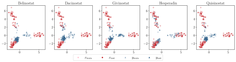
Figure 6: Overview of the single cell dataset Srivatsan et al. [2020]. We show the first two PCA dimensions performed on the training data, and limit the figure to 50 samples. The point cloud $({\mathbf{x}}_{\mathrm{train}},{\mathbf{x}}_{\mathrm{test}})$ shows the control cells and $({\mathbf{y}}_{\mathrm{train}},{\mathbf{y}}_{\mathrm{test}})$ are the perturbed cells using a specific drug.

Comparing Map Estimators on Single-Cell Data. We consider the sci-Plex single-cell RNA sequencing data from (Srivatsan et al., 2020) which contains the responses of cancer cell lines to 188 drug perturbations, as reflected in their gene expression. Visualized in Figure 6, we focus on $5$ drugs (Belinostat, Dacinostat, Givinostat, Hesperadin, and Quisinostat) which have a significant impact on the cell population as reported by Srivatsan et al. (2020). We remove genes which appear in less than 20 cells, and discard cells which have an incomplete gene expression of less than 20 genes, obtaining $n\approx 10^{4}$ source and $m\approx 500$ target cells, depending on the drug. We whiten the data, take it to $\log(1+x)$ scale and apply PCA to reduce the dimensionality to $d=\{16,64,256\}$. This procedure repeats the pre-processing steps of Cuturi et al. (2023).

We consider four baselines: (1) training an input convex neural network (ICNN) (Amos et al., 2017) using the objective of Amos (2022) (2) training a feed-forward neural network regularized with the Monge Gap (Uscidda and Cuturi, 2023), (3) instantiating the entropic map estimator (Pooladian and Niles-Weed, 2021) and (4) its debiased variant (Feydy et al., 2019; Pooladian et al., 2022). The first two algorithms use neural networks, and we follow hyper-parameter tuning in (Uscidda and Cuturi, 2023). We choose the number of hidden layers for both as $[128,64,64]$. For the ICNN we use a learning rate $\eta=10^{-3}$, batch size $b=256$ and train it using the Adam optimizer (Kingma and Ba, 2014) for $2000$ iterations. For the Monge Gap we set the regularization constant $\lambda_{\mathrm{MG}}=10$, $\lambda_{\mathrm{cons}}=0.1$ and the Sinkhorn regularization to $\varepsilon=0.01$. We train the Monge Gap in a similar setting, except that we set $\eta=0.01$. To choose $\varepsilon$ for entropic estimators, we split the training data to get an evaluation set and perform $5$-fold cross-validation on the grid of $\{2^{-3},\dots,2^{3}\}\times\varepsilon_{0}$, where $\varepsilon_{0}$ is computed as in line 2 of Algorithm 4.

We compare the algorithms by their ability to align the population of control cells, to cells treated with a drug. We randomly split the data into $80\%-20\%$ train and test sets, and report the mean and standard error of performance over the test set, for an average of 5 runs. Detailed in Table 1, ProgOT outperforms the baselines consistently with respect to $D_{\varepsilon_{D}}((\mathscr{T}_{\mathrm{Prog}})_{\#}{\mathbf{X}},{\mathbf{Y}})$. The table shows complete results for $3$ drugs, and the overall ranking based on performance across all $5$ drugs.

Table 1: Performance of ProgOT compared to baselines, w.r.t $\mathrm{D}_{\varepsilon_{D}}$ between source and target of the sci-Plex dataset. Reported numbers are the average of 5 runs, together with the standard error.

Drug	Belinostat			Givinostat			Hesperadin			5-drug rank
$d_{\mathrm{PCA}}$	16	64	256	16	64	256	16	64	256
ProgOT	2.9$\pm$0.1	8.8$\pm$0.1	20.8$\pm$0.2	3.3$\pm$0.2	9.0$\pm$0.3	21.9$\pm$0.3	3.7$\pm$0.4	10.1$\pm$0.4	23.1$\pm$0.4	1
EOT	2.5$\pm$0.1	9.6$\pm$0.1	22.8$\pm$0.2	3.9$\pm$0.4	10.0$\pm$0.1	24.7$\pm$0.9	4.1$\pm$0.4	10.4$\pm$0.5	26$\pm$1.3	2
Debiased EOT	3.2$\pm$0.1	14.3$\pm$0.1	39.8$\pm$0.4	3.7$\pm$0.2	14.7$\pm$0.1	42.4$\pm$0.8	4.0$\pm$0.5	15.2$\pm$0.6	41$\pm$1.1	4
Monge Gap	3.1$\pm$0.1	10.3$\pm$0.1	34.4$\pm$0.3	2.8$\pm$0.2	9.9$\pm$0.2	34.9$\pm$0.3	3.7$\pm$0.5	11.0$\pm$0.5	36$\pm$1.1	3
ICNN	5.0$\pm$0.1	14.7$\pm$ 0.1	42$\pm$1	5.1$\pm$0.1	14.8$\pm$0.2	40.3$\pm$0.1	4.0$\pm$0.4	14.4$\pm$0.5	46$\pm$2.1	5

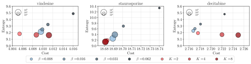
Figure 5: Performance as a coupling solver on the 4i dataset. ProgOT returns better couplings, in terms of the OT cost and the entropy, for a fraction of Sinkhorn iterations, while still returning a coupling that has the same deviation to the original marginals. The (top) row is computed using $h=\|.\|^{2}_{2}$, the (bottom) row shows results for the cost $h=\tfrac{1}{p}\|\cdot\|^{p}_{p}$ where $p=1.5$.

5.2 ProgOT as a Coupling Solver

In this section, we benchmark the ability of ProgOT to return a coupling, and compare it to that of the Sinkhorn algorithm. Comparing coupling solvers is rife with challenges, as their time performance must be compared comprehensively by taking into account three crucial metrics: (i) the cost of transport according to the coupling $\mathbf{P}$, that is, $\langle\mathbf{P},\mathbf{C}\rangle$, (ii) the entropy $E(\mathbf{P})$, and (iii) satisfaction of marginal constraints $\|\mathbf{P}\mathbf{1}_{m}-\mathbf{a}\|_{1}+\|\mathbf{P}^{T}\mathbf{1}_{n}-\mathbf{b}\|_{1}$. Due to our threshold schedule $(\tau_{k})_{k}$, as detailed in Section 4, both approaches are guaranteed to output couplings that satisfy the same threshold for criterion (iii), leaving us only three quantities to monitor: compute effort here quantified as total number of Sinkhorn iterations, summed over all $K$ steps for ProgOT), transport cost and entropy. While compute effort and transport cost should, ideally, be as small as possible, certain applications requiring, e.g., differentiability (Cuturi et al., 2019) or better sample complexity (Genevay et al., 2019), may prefer higher entropies.

To monitor these three quantities, and cover an interesting space of solutions that, we run Sinkhorn’s algorithm for a logarithmic grid of $\varepsilon=\beta\varepsilon_{0}$ values (here $\varepsilon_{0}$ is defined in Line 2 of Algorithm 4), and compare it to constant-speed ProgOT with $K=\{2,4,8\}$. Because one cannot compare these regularizations, we explore many choices to schedule $\varepsilon$ within ProgOT. Following the default strategy used in OTT-JAX (Cuturi et al., 2022a), we set at every iterate $k$, $\varepsilon_{k}=\theta\bar{c}_{k}$, where $\bar{c}_{k}$ is 5% of the the mean of the cost matrix at that iteration, as detailed in Appendix A. We do not use Algorithm 4 since it returns a regularization schedule that is tuned for map estimation, while the goal here is to recover couplings that are comparable to those outputted by Sinkhorn. We set the threshold for marginal constraint satisfaction for both algorithms as $\tau_{K}=\tau=0.001$ and run all algorithms to convergence, with infinite iteration budget. For the coupling experiments, we use the single-cell multiplex data of Bunne et al. (2023), reflecting morphological features and protein intensities of melanoma tumor cells. The data describes $d=47$ features for $n\approx 11,000$ control cells, and $m\approx 2,800$ treated cells, for each of 34 drugs, of which we use only 6 at random. To align the cell populations, we consider two ground costs: the squared-Euclidean norm $\|\cdot\|^{2}$ as well as $h=\tfrac{1}{p}\|\cdot\|_{p}^{p}$, with $p=1.5$.

Results for $6$ drugs are displayed in Figure 5. The area of the marker reflects the total number of Sinkhorn iterations needed for either algorithm to converge to a coupling with a threshold $\tau=10^{-3}$. The values for $\beta$ and $K$ displayed in the legend are encoded using colors. The global scaling parameter for ProgOT is set to $\theta=2^{-4}$. Figure 8 and 9 visualize other choices for $\theta$. These results prove that ProgOT provides a competitive alternative to Sinkhorn, to compute couplings that yield a small entropy and cost at a low computational effort, while satisfying the same level of marginal constraints.

Conclusion

In this work, we proposed ProgOT, a new family of EOT solvers that blend dynamic and static formulations of OT by using the Sinkhorn algorithm as a subroutine within a progressive scheme. ProgOT aims to provide practitioners with an alternative to the Sinkhorn algorithm that (i) does not fail when instantiated with uninformed or ill-informed $\varepsilon$ regularization, thanks to its self-correcting behavior and our simple $\varepsilon$-scheduling scheme that is informed by the dispersion of the target distribution, (ii) performs at least as fast as Sinkhorn when used to compute couplings between point clouds, and (iii) provides a reliable out-of-the-box OT map estimator that comes with a non-asymptotic convergence guarantee. We believe ProgOT can be used as a strong baseline to estimate Monge maps.

Appendix A Additional Experiments and Details

Generation of Figure 1 and Figure 2. We consider a toy example where the target and source clouds are as shown in Figure 1. We visualize the entropic map [Pooladian and Niles-Weed, 2021], its debiased variant [Pooladian et al., 2022] and ProgOT, where we consider a decelerated schedule with $6$ steps, and only visualize steps $k=3,5$ to avoid clutter. The hyperparameters of the algorithms are set as described in Section 5. Figure 2 shows the coupling matrix corresponding to the same data, resulting from the same solvers.

Sinkhorn Divergence and its Regularization Parameter. In some of the experiments, we calculate the Sinkhorn divergence between two point clouds as a measure of distance. In all experiments we set the value of $\varepsilon_{D}$ and according to the geometry of the target point cloud. In particular, we set $\varepsilon$ to be default value of the OTT-JAX Cuturi et al. [2022b] library for this point cloud via ott.geometry.pointcloud.PointCloud(Y).epsilon, that is, $5\%$ of the average cost matrix, within the target points.

Details of Scheduling $(\alpha_{k})_{k}$. Table 2 specifies our choices of $\alpha_{k}$ for the three schedules detailed in Section 4. Figure 7 compares the performance of ProgOT with constant-speed schedule in red, with the decelerated (Dec.) schedules in green. The figure shows results on the sci-Plex data (averaged across 5 drugs) and the Gaussian Mixture synthetic data. We observe that the algorithms perform roughly on par, implying that in practice ProgOT is robust to choice of $\alpha$.

Table 2: Scheduling Schemes for $\alpha_{k}$.

Schedule	$\alpha_{k}=\alpha(k)$	$t_{k}=t(k)$
Decelerated	$1/e$	$\frac{1-e^{-(k+1)}}{e-1}$
Constant-Speed	$\frac{1}{K-k+2}$	$\frac{k}{K}$
Accelerated	$\frac{2k-1}{(K+1)^{2}-(k-1)^{2}}$	$\left(\frac{k}{K}\right)^{2}$

Details of Scheduling $(\varepsilon_{k})_{k}$. For map experiments on the sci-Plex data [Srivatsan et al., 2020], we schedule the regularization parameters via Algorithm 4. We set $\beta_{0}=5$ and consider the set $s_{p}=\{0.1,0.5,1,5,10,20\}$. For coupling experiments on the 4i data [Gut et al., 2018] we set the regularizations as follows. Let ${\mathbf{x}}_{1}^{(k)},\dots,{\mathbf{x}}_{n}^{(k)}$ denote the interpolated point cloud at iterate $k$ (according to Line 7, Algorithm 2) and recall that ${\mathbf{y}}_{1},\dots,{\mathbf{y}}_{m}$ is the target point cloud. The scaled average cost at this iterate is $\bar{c}_{k}=\sum_{i,j}h({\mathbf{x}}^{(k)}_{i}-{\mathbf{y}}_{j})/(20mn)$, which is the default value of $\varepsilon$ typically used for running Sinkhorn. Then for every $k\in[K]$, we set $\varepsilon_{k}=\theta\bar{c}_{k}$ to make ProgOT compatible to the $\beta$ regularization levels of the benchmarked Sinkhorn algorithms. For Figure 5, we have set $\theta=2^{-4}$. In Figure 8 and Figure 9, we visualize the results for $\theta\in\{2^{-7},2^{-4},2^{-1}\}$ to give an overview of the results using small and larger scaling values.

Compute Resources. Experiments were run on a single Nvidia A100 GPU for a total of 24 hours. Smaller experiments and debugging was performed on a single MacBook M2 Max.

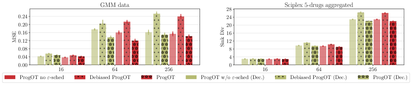
Figure 7: Comparison of constant speed vs decelerated ProgOT.

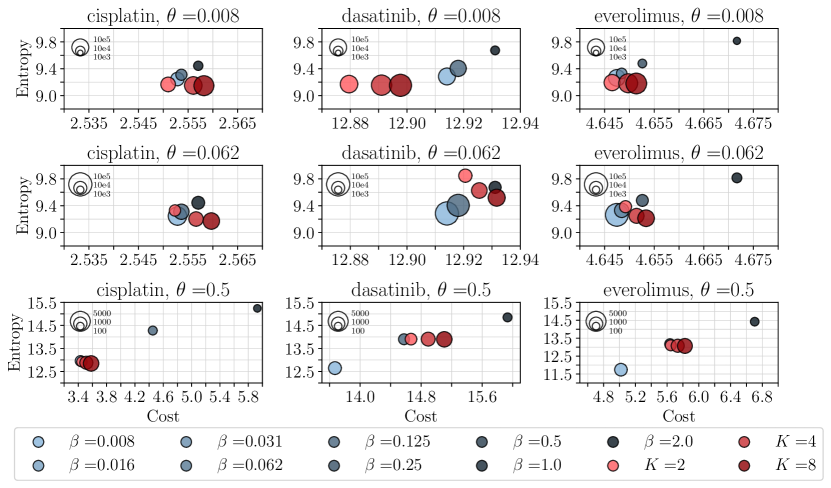
Figure 8: Comparison of ProgOT and Sinkhorn as coupling solvers for $h(\cdot)=\|\cdot\|_{2}^{2}$. Different rows show different choice of regularization $\theta$ for ProgOT as detailed in Appendix A.

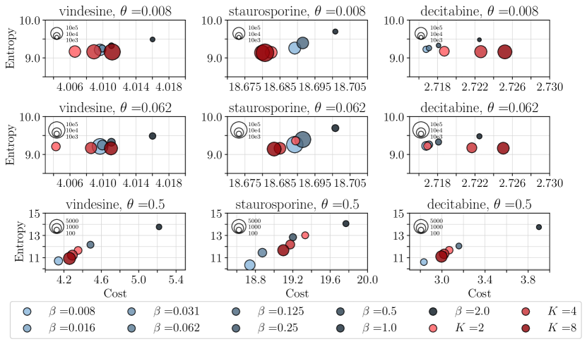
Figure 9: Comparison of ProgOT and Sinkhorn as coupling solvers for $h=\|\cdot\|_{1.5}^{1.5}/1.5$. Different rows show different choice of regularization $\theta$ for ProgOT as detailed in Appendix A.

Appendix B Proofs

Preliminaries.

Before proceeding with the proofs, we collect some basic definitions and facts. First, we write the the $p$-Wasserstein distance for any $p\geq 1$:

$$W_{p}(\mu,\nu)\coloneqq\Bigl{(}\inf_{\pi\in\Pi(\mu,\nu)}\iint\|x-y\|^{p}\mathrm{d}\pi(x,y)\Bigr{)}^{1/p}\,.$$

Moreover, it is well-known that $p$-Wasserstein distances are ordered for $p\geq 1$: for $1\leq p\leq q$, it holds that $W_{p}(\mu,\nu)\leq W_{q}(\mu,\nu)$ [cf. Remark 6.6, Villani et al., 2009].

For the special case of the $1$-Wasserstein distance, we have the following dual formulation

$$W_{1}(\mu,\nu)=\sup_{f\in\text{Lip}_{1}}\int f\mathrm{d}(\mu-\nu)\,,$$

where $\text{Lip}_{1}$ is the space of $1$-Lipschitz functions [cf. Theorem 5.10, Villani et al., 2009].

Returning to the $2$-Wasserstein distance, we will repeatedly use the following two properties of optimal transport maps. First, for any two measures $\mu,\nu$ and an $L$-Lipschitz map $T$, it holds that

$$W_{2}(T_{\#}\mu,T_{\#}\nu)\leq LW_{2}(\mu,\nu)\,.$$ (9)

This follows from a coupling argument. In a similar vein, we will use the following upper bound on the Wasserstein distance between the pushforward of a source measure $\mu$ by two different optimal transport maps $T_{a}$ and $T_{b}$:

$$W_{2}^{2}((T_{a})_{\#}\mu,(T_{b})_{\#}\mu)\leq\|T_{a}-T_{b}\|^{2}_{L^{2}(\mu)}\,,$$ (10)

Notation conventions.

For an integer $K\in\mathbb{N}$, $[K]\coloneqq\{0,\ldots,K\}$. We write $a\lesssim b$ to mean that there exists a constant $C>0$ such that $a\leq Cb$. A constant can depend on any of the quantities present in (A1) to (A3), as well as the support of the measures, and the number of iterations in Algorithm 2. The notation $a\lesssim_{\log(n)}b$ means that $a\leq C_{1}(\log n)^{C_{2}}b$ for positive constants $C_{1}$ and $C_{2}$.

B.1 Properties of entropic maps

Before proving properties of the entropic map, we first recall the generalized form of (2), which holds for arbitrary measures (cf. Genevay [2019]):

$$\sup_{(f,g)\in L^{1}(\mu)\times L^{1}(\nu)}\int f\mathrm{d}\mu+\int g\mathrm{d}\nu-\varepsilon\iint e^{(f(x)+g(y)-\tfrac{1}{2}\|x-y\|^{2})/\varepsilon}\mathrm{d}\mu(x)\mathrm{d}\nu(y)+\varepsilon\,.$$ (11)

When the entropic dual formulation admits maximixers, we denote them by $(f_{\varepsilon},g_{\varepsilon})$ and refer to them as optimal entropic Kantorovich potentials [e.g., Genevay, 2019, Theorem 7]. Such potentials always exist if $\mu$ and $\nu$ have compact support.

We can express an entropic approximation to the optimal transport coupling $\pi_{0}$ as a function of the dual maximizers [Csiszár, 1975]:

$$\pi_{\varepsilon}(x,y)\coloneqq\gamma_{\varepsilon}(x,y)\mathrm{d}\mu(x)\mathrm{d}\nu(y)\coloneqq\exp\Bigl{(}\frac{f_{\varepsilon}(x)+g_{\varepsilon}(y)-\tfrac{1}{2}\|x-y\|^{2}}{\varepsilon}\Bigr{)}\mathrm{d}\mu(x)\mathrm{d}\nu(y)\,.$$ (12)

When necessary, we will be explicit about the measures that give rise to the entropic coupling. For example, in place of the above, we would write

$$\pi_{\varepsilon}^{\mu\to\nu}(x,y)=\gamma_{\varepsilon}^{\mu\to\nu}(x,y)\mathrm{d}\mu(x)\mathrm{d}\nu(y)\,.$$ (13)

The population counterpart to (7), the entropic map from $\mu$ to $\nu$, is then expressed as

$$T_{\varepsilon}^{\mu\to\nu}(x)\coloneqq{\mathbb{E}}_{\pi_{\varepsilon}}[Y|X=x]\,,$$

and similarly the entropic map from $\nu$ to $\mu$ is

$$T_{\varepsilon}^{\nu\to\mu}(y)\coloneqq{\mathbb{E}}_{\pi_{\varepsilon}}[X|Y=y]\,.$$

We write the forward (resp. backward) entropic Brenier potentials as $\varphi_{\varepsilon}\coloneqq\tfrac{1}{2}\|\cdot\|^{2}-f_{\varepsilon}$ (resp. $\psi_{\varepsilon}\coloneqq\tfrac{1}{2}\|\cdot\|^{2}-g_{\varepsilon}$). By dominated convergence, one can verify that

$$\nabla\varphi_{\varepsilon}(x)=T^{\mu\to\nu}_{\varepsilon}(x)\,,\quad\nabla\psi_{\varepsilon}(y)=T^{\nu\to\mu}_{\varepsilon}(y)\,.$$

We now collect some general properties of the entropic map, which we state over the ball but can be readily generalized.

Lemma 5.

Let $\mu,\nu$ be probability measures over $B(0;R)$ in ${\mathbb{R}}^{d}$. Then for a fixed $\varepsilon>0$, it holds that both $T^{\mu\to\nu}_{\varepsilon}$ and $T^{\nu\to\mu}_{\varepsilon}$ are Lipschitz with constant upper-bounded by $R^{2}/\varepsilon$.

Proof of Lemma 5.

We prove only the case for $T^{\mu\to\nu}_{\varepsilon}$ as the proof for the other map is completely analogous. It is well-known that the Jacobian of the map is a symmetric positive semi-definite matrix: $\nabla T_{\varepsilon}^{\mu\to\nu}(x)=\varepsilon^{-1}\text{Cov}_{\pi_{\varepsilon}}(Y|X=x)$ (see e.g., Chewi and Pooladian [2023, Lemma 1]). Since the probability measures are supported in a ball of radius $R$, it holds that $\sup_{x}\|\text{Cov}_{\pi_{\varepsilon}}(Y|X=x)\|_{\text{op}}\leq R^{2}$, which completes the claim. ∎

We also require the following results from Divol et al. [2024], as well as the following object: for three measures $\rho,\mu,\nu$ with finite second moments, write

$$\bar{I}\coloneqq\iiint\log\Bigl{(}\frac{\gamma^{\rho\to\mu}_{\varepsilon}(x,y)}{\gamma^{\rho\to\nu}_{\varepsilon}(x,z)}\Bigr{)}\gamma^{\rho\to\mu}_{\varepsilon}(x,y)\mathrm{d}\pi(y,z)\mathrm{d}\rho(x)\,,$$

where $\pi$ is an optimal transport coupling for the $2$-Wasserstein distance between $\mu$ and $\nu$, and $\gamma_{\varepsilon}$ is the density defined in (13).

Lemma 6.

[Divol et al., 2024, Proposition 3.7 and Proposition 3.8] Suppose $\rho,\mu,\nu$ have finite second moments, then

$$\varepsilon\bar{I}\leq\iint\langle T_{\varepsilon}^{\mu\to\rho}(y)-T_{\varepsilon}^{\nu\to\rho}(z),y-z\rangle\mathrm{d}\pi(y,z)\,,$$

and

$$\iint\|T_{\varepsilon}^{\mu\to\rho}(y)-T_{\varepsilon}^{\nu\to\rho}(z)\|^{2}\mathrm{d}\pi(y,z)\leq 2\bar{I}\sup_{v\in{\mathbb{R}}^{d}}\|\mathrm{Cov}_{\pi_{\varepsilon}^{\rho\to\nu}}(X|Y=v)\|_{\mathrm{op}}\,.$$

We are now ready to prove Proposition 4. We briefly note that stability of entropic maps and couplings has been investigated by many [e.g., Ghosal et al., 2022, Eckstein and Nutz, 2022, Carlier et al., 2024]. These works either present qualitative notions of stability, or give bounds that depend exponentially on $1/\varepsilon$. In contrast, the recent work of Divol et al. [2024] proves that the entropic maps are Lipschitz with respect to variations of the target measure, where the underlying constant is linear in $1/\varepsilon$. We show that their result also encompasses variations in the source measure, which is of independent interest.

Proof of Proposition 4.

Let $\pi\in\Gamma(\mu,\mu^{\prime})$ be the optimal transport coupling from $\mu$ to $\mu^{\prime}$. By disintegrating and applying the triangle inequality, we have

$$\int\|T_{\varepsilon}^{\mu\to\rho}(x)-T_{\varepsilon}^{\mu^{\prime}\to\rho}(x)\|\mathrm{d}\mu(x) =\iint\|T_{\varepsilon}^{\mu\to\rho}(x)-T_{\varepsilon}^{\mu^{\prime}\to\rho}(x)\|\mathrm{d}\pi(x,x^{\prime})$$

$$\leq\iint\|T_{\varepsilon}^{\mu\to\rho}(x)-T_{\varepsilon}^{\mu^{\prime}\to\rho}(x^{\prime})\|\mathrm{d}\pi(x,x^{\prime})$$

$$\qquad\qquad+\|T_{\varepsilon}^{\mu^{\prime}\to\rho}(x)-T_{\varepsilon}^{\mu^{\prime}\to\rho}(x^{\prime})\|\mathrm{d}\pi(x,x^{\prime})$$

$$\leq\iint\|T_{\varepsilon}^{\mu\to\rho}(x)-T_{\varepsilon}^{\mu^{\prime}\to\rho}(x^{\prime})\|\mathrm{d}\pi(x,x^{\prime})$$

$$\qquad\qquad+\frac{R^{2}}{\varepsilon}\iint\|x-x^{\prime}\|\mathrm{d}\pi(x,x^{\prime})$$

$$\leq\iint\|T_{\varepsilon}^{\mu\to\rho}(x)-T_{\varepsilon}^{\mu^{\prime}\to\rho}(x^{\prime})\|\mathrm{d}\pi(x,x^{\prime})+\frac{R^{2}}{\varepsilon}W_{2}(\mu,\mu^{\prime})\,,$$

where the penultimate inequality follows from Lemma 5, and the last step is due to Jensen’s inequality. To bound the remaining term, recall that

$$\sup_{v\in{\mathbb{R}}^{d}}\|\text{Cov}_{\pi_{\varepsilon}^{\rho\to\nu}}(X|Y=v)\|_{\text{op}}\leq R^{2}\,,$$

and by the two inequalities in Lemma 6, we have (replacing $\nu$ with $\mu^{\prime}$)

$$\iint\|T_{\varepsilon}^{\mu\to\rho}(x)-T_{\varepsilon}^{\mu^{\prime}\to\rho}(x^{\prime})\|^{2}\mathrm{d}\pi(x,x^{\prime}) \leq 2\bar{I}R^{2}$$

$$=\frac{2R^{2}}{\varepsilon}(\varepsilon\bar{I})$$

$$\leq\frac{2R^{2}}{\varepsilon}\iint\langle T_{\varepsilon}^{\mu\to\rho}(y)-T_{\varepsilon}^{\mu^{\prime}\to\rho}(z),y-z\rangle\mathrm{d}\pi(y,z)$$

$$\leq\frac{2R^{2}}{\varepsilon}\Bigl{(}\iint\|T_{\varepsilon}^{\mu\to\rho}(x)-T_{\varepsilon}^{\mu^{\prime}\to\rho}(x^{\prime})\|\mathrm{d}\pi(x,x^{\prime})\Bigr{)}W_{2}(\mu,\mu^{\prime})\,,$$

where we used Cauchy-Schwarz in the last line. An application of Jensen’s inequality and rearranging results in the bound:

$$\iint\|T_{\varepsilon}^{\mu\to\rho}(x)-T_{\varepsilon}^{\mu^{\prime}\to\rho}(x^{\prime})\|\mathrm{d}\pi(x,x^{\prime})\leq\frac{2R^{2}}{\varepsilon}W_{2}(\mu,\mu^{\prime})\,,$$

which completes the claim. ∎

Finally, we require the following results from Pooladian and Niles-Weed [2021], which we restate for convenience but under our assumptions.

Lemma 7.

[Two-sample bound: Pooladian and Niles-Weed, 2021, Theorem 3] Consider i.i.d. samples of size $n$ from each distribution $\mu$ and $\nu$, resulting in the empirical measures $\hat{\mu}$ and $\hat{\nu}$, with the corresponding. Let $\hat{T}_{\varepsilon}$ be the entropic map between $\hat{\mu}$ and $\hat{\nu}$. Under (A1)-(A3), it holds that

$$\mathbb{E}\,\left\lVert\hat{T}_{\varepsilon}-T_{0}\right\rVert_{L^{2}(\mu)}^{2}\lesssim_{\log(n)}\varepsilon^{-d/2}n^{-1/2}+\varepsilon^{2}\,.$$

Moreover, if $\varepsilon=\varepsilon(n)\asymp n^{-1/(d+4)}$, then the overall rate of convergence is $n^{-2/(d+4)}$.

Lemma 8.

[One-sample bound: Pooladian and Niles-Weed, 2021, Theorem 4] Consider i.i.d. samples of size $n$ from $\nu$, resulting in the empirical measure $\hat{\nu}$, with full access to a probability measure $\mu$. Let $\hat{R}_{\varepsilon}$ be the entropic map from $\mu$ to $\hat{\nu}$. Under (A1)-(A3), it holds that

$$\mathbb{E}\,\left\lVert\hat{R}_{\varepsilon}-T_{0}\right\rVert_{L^{2}(\mu)}^{2}\lesssim_{\log(n)}\varepsilon^{1-d/2}n^{-1/2}+\varepsilon^{2}\,.$$

Moreover, if $\varepsilon=\varepsilon(n)\asymp n^{-1/(d+2)}$, then the overall rate of convergence is $n^{-2/(d+2)}$.

B.2 Remaining ingredients for the proof of Theorem 3

We start by analyzing our Progressive OT map estimator between the iterates. We will recurse on these steps, and aggregate the total error at the end. We introduce some concepts and shorthand notations.

First, the ideal progressive Monge problem: Let $T^{(0)}$ be the optimal transport map from $\mu$ to $\nu$, and write $\mu^{(0)}\coloneqq\mu$. Then write

$$S^{(0)}\coloneqq(1-\alpha_{0})\operatorname{Id}+\alpha_{0}T^{(0)}\,,$$

and consequently $\mu^{(1)}\coloneqq(S^{(0)})_{\#}\mu^{(0)}$. We can iteratively define $T^{(i)}$ to be the optimal transport map from $\mu^{(i)}$ to $\nu$, and consequently

$$S^{(i)}\coloneqq(1-\alpha_{i})\operatorname{Id}+\alpha_{i}T^{(i)}\,,$$

and thus $\mu^{(i+1)}\coloneqq(S^{(i)})_{\#}\mu^{(i)}$. The definition of McCann interpolation implies that these iterates all lie on the geodesic between $\mu$ and $\nu$. This ideal progressive Monge problem precisely mimicks our progressive map estimator, though (1) these quantities are defined at the population level, and (2) the maps are defined a solutions to the Monge problem, rather than its entropic analogue. Recall that we write $\hat{\mu}$ and $\hat{\nu}$ as the empirical measures associated with $\mu$ and $\nu$, and recursively define $\mathscr{E}^{(i)}$ to be the entropic map from $\hat{\mu}^{(i)}_{\varepsilon}$ to $\hat{\nu}$, where $\hat{\mu}^{(0)}_{\varepsilon}\coloneqq\hat{\mu}$, and

$$\hat{\mu}_{\varepsilon}^{(i+1)}\coloneqq(\mathscr{S}^{(i)})_{\#}\hat{\mu}_{\varepsilon}^{(i)}\coloneqq((1-\alpha_{i})\operatorname{Id}+\alpha_{i}\mathscr{E}^{(i)})_{\#}\hat{\mu}_{\varepsilon}^{(i)}\,.$$ (14)

We also require $\hat{R}_{\varepsilon}^{(i)}$, defined to be the the entropic map between $\mu^{(i)}$ and $\hat{\nu}$ using regularization $\varepsilon_{i}$. This map can also be seen as a “one-sample" estimator, which starts from iterates of the McCann interpolation, and maps to an empirical target distribution.

To control the performance of $\hat{R}_{\varepsilon}^{(i)}$ below, we want to use Lemma 8. To do so, we need to verify that $\mu^{(i)}$ also satisfies the key assumptions (A1) to (A3). This is accomplished in the following lemma.

Lemma 9 (Error rates for $\hat{R}_{\varepsilon}^{(i)}$).

For any $i\geq 0$, the measures $\mu^{(i)}$ and $\nu$ continue to satisfy (A1) to (A3), and thus

$${\mathbb{E}}\|\hat{R}_{\varepsilon}^{(i)}-T_{0}\|^{2}_{L^{2}(\mu^{(i)})}\lesssim\varepsilon_{i}^{1-d/2}n^{-1/2}+\varepsilon_{i}^{2}\,.$$

Proof.

We verify that the conditions (A1) to (A3) hold for the pair $(\mu^{(1)},\nu)$; repeating the argument for the other iterates is straightforward.

First, we recall that for two measures $\mu_{0}\coloneqq\mu,\mu_{1}\coloneqq\nu$ with support in a convex subset $\Omega\subseteq{\mathbb{R}}^{d}$, the McCann interpolation $(\mu_{\alpha})_{\alpha\in[0,1]}$ remains supported in $\Omega$; see Santambrogio [2015, Theorem 5.27]. Moreover, by Proposition 7.29 in Santambrogio [2015], it holds that

$$\|\mu_{\alpha}\|_{L^{\infty}(\Omega)}\leq\max\{\|\mu_{0}\|_{L^{\infty}(\Omega)},\|\mu_{1}\|_{L^{\infty}(\Omega)}\}\leq\max\{\mu_{\max},\nu_{\max}\}\,,$$

for any $\alpha\in[0,1]$, recall that the quantities $\mu_{\max},\nu_{\max}$ are from (A1). Thus, the density of $\mu^{(1)}=\mu_{\alpha_{0}}=((1-\alpha_{0})\operatorname{Id}+\alpha_{0}T)_{\#}\mu$ is uniformly upper bounded on $\Omega$; altogether this covers (A1). For (A2) and (A3), note that we are never leaving the geodesic. Rather than study the “forward” map, we can therefore instead consider the “reverse" map

$$\bar{T}\coloneqq(\alpha_{0}\operatorname{Id}+(1-\alpha_{0})T^{-1})\,,$$

which satisfies ${\bar{T}}_{\#}\nu=\mu^{(1)}$ and hence $T^{(1)}=\bar{T}^{-1}$. We now verify the requirements of (A2) and (A3). For (A2), since $(T^{(1)})^{-1}=\bar{T}=\alpha_{0}\operatorname{Id}+(1-\alpha_{0})T^{-1}$, and $T^{-1}$ is three-times continuously differentiable by assumption, the map $(T^{(1)})^{-1}$ is also three times continuously differentiable, with third derivative bounded by that of $T^{-1}$. For (A3), we use the fact that $T=\nabla\varphi_{0}$ for some function $\varphi_{0}$ which is $\Lambda$-smooth and $\lambda$-strongly convex. Basic properties of convex conjugation then imply that $T^{(1)}=\nabla\varphi_{1}$, where $\varphi_{1}=(\alpha_{0}\tfrac{\|\cdot\|^{2}}{2}+(1-\alpha_{0})\varphi_{0}^{*})^{*}$. Since the conjugate of a $\lambda$-strongly convex function is $\lambda^{-1}$-smooth, and conversely, we obtain that the function $\varphi_{1}$ is $(\alpha_{0}+(1-\alpha_{0})\lambda^{-1})^{-1}$ strongly convex and $(\alpha_{0}+(1-\alpha_{0})\Lambda^{-1})^{-1}$. In particular, since $(\alpha_{0}+(1-\alpha_{0})\lambda^{-1})^{-1}\geq\min(1,\lambda)$ and $(\alpha_{0}+(1-\alpha_{0})\Lambda^{-1})^{-1}\leq\max(1,\Lambda)$, we obtain that $DT^{(1)}$ is uniformly bounded above and below. ∎

We define the following quantities which we will recursively bound:

$$\Delta_{i}\coloneqq{\mathbb{E}}\|\mathscr{E}^{(i)}-T^{(i)}\|^{2}_{L^{2}(\mu^{(i)})}\,,\Delta_{R_{i}}\coloneqq\|\hat{R}_{\varepsilon}^{(i)}-T^{(i)}\|^{2}_{L^{2}(\mu^{(i)})}\,,\mathbb{W}_{i}\coloneqq{\mathbb{E}}W_{2}^{2}(\hat{\mu}_{\varepsilon}^{(i)},\mu^{(i)})\,,$$ (15)

as well as

$$\mathcal{A}_{i}\coloneqq 1-\alpha_{i}+R^{2}\frac{\alpha_{i}}{\varepsilon_{i}}\,,$$

where recall $R$ is the radius of the ball $B(0;R)$ in ${\mathbb{R}}^{d}$.

First, the following lemma:

Lemma 10.

If the support of $\mu$ and $\nu$ is contained in $B(0;R)$ and $\alpha_{i}\lesssim\varepsilon_{i}$ for $i=0,\dots,k$, then

$$\left\lVert\mathscr{T}_{\mathrm{Prog}}^{(k)}-T_{0}\right\rVert^{2}_{L^{2}(\mu)}\lesssim\sum_{i=0}^{k}\Delta_{i}\,.$$

Proof.

We prove this lemma by iterating over the quantity defined by

$$E_{j}\coloneqq\left\lVert\mathscr{E}^{(k)}\circ\mathscr{S}^{(k-1)}\circ\dots\circ\mathscr{S}^{(j)}-T^{(k)}\circ S^{(k-1)}\circ\dots\circ S^{(j)}\right\rVert^{2}_{L^{2}(\mu^{(j)})}.$$

when $j\leq k-1$ and $E_{k}=\Delta_{k}$. By adding and subtracting $S^{(j)}$ and $\hat{S}_{\varepsilon}^{(j)}$ appropriately, we obtain for $j\leq k-1$,

$$E_{j} \lesssim\left\lVert\mathscr{E}^{(k)}\circ\mathscr{S}^{(k-1)}\circ\dots\circ\mathscr{S}^{(j)}-\mathscr{E}^{(k)}\circ\mathscr{S}^{(k-1)}\circ\dots\circ\mathscr{S}^{(j+1)}\circ S^{(j)}\right\rVert^{2}_{L^{2}(\mu^{(j)})}$$

$$\qquad\qquad+\left\lVert\mathscr{E}^{(k)}\circ\mathscr{S}^{(k-1)}\circ\dots\circ\mathscr{S}^{(j+1)}\circ S^{(j)}-T^{(k)}\circ S^{(k-1)}\circ\dots\circ S^{(j)}\right\rVert^{2}_{L^{2}(\mu^{(j)})}$$

$$\leq\left(\alpha_{j}\mathrm{Lip}(\mathscr{E}^{(k)})\mathrm{Lip}(\mathscr{S}^{(k-1)})\dots\mathrm{Lip}(\mathscr{S}^{(j+1)})\right)^{2}\Delta_{j}+E_{j+1}$$

$$\lesssim\left(\frac{\alpha_{j}}{\varepsilon_{k}}\prod_{l=j+1}^{k-1}\mathcal{A}_{\ell}\right)^{2}\Delta_{j}+E_{j+1}$$

$$\lesssim\Delta_{j}+E_{j+1}$$

where in the last inequality we have used the fact that $\alpha_{j}\lesssim\varepsilon_{j}$, so that $\mathcal{A}_{k}\lesssim 1$ for all $k$. Repeating this process yields $\left\lVert\mathscr{T}_{\mathrm{Prog}}^{(k)}-T_{0}\right\rVert^{2}_{L^{2}(\mu)}=E_{0}\lesssim\sum_{i=0}^{k}\Delta_{k}$, which completes the proof. ∎

To prove Theorem 3, it therefore suffices to bound $\Delta_{k}$. We prove the following lemma by induction, which gives the proof.

Lemma 11.

Assume $d\geq 4$. Suppose (A1) to (A3) hold, and $\alpha_{i}\asymp n^{-1/d}$ and $\varepsilon_{i}\asymp n^{-1/2d}$ for all $i\in[k]$. Then it holds that for $k\geq 0$,

$$\mathbb{W}_{k}\lesssim_{\log(n)}n^{-2/d}\,,\quad\text{and}\quad\Delta_{k}\lesssim_{\log(n)}n^{-1/d}\,.$$

Proof.

We proceed by induction. For the base case $k=0$, the bounds of Fournier and Guillin [2015] imply that $\mathbb{W}_{0}={\mathbb{E}}[W_{2}^{2}(\hat{\mu},\mu)]\lesssim n^{-2/d}$. Similarly, by Lemma 7, we have $\Delta_{0}\lesssim_{\log(n)}\varepsilon_{0}^{-d/2}n^{-1/2}+\varepsilon_{0}^{2}\lesssim_{\log(n)}n^{-1/d}$.

Now, assume that the claimed bounds hold for $\mathbb{W}_{k}$ and $\Delta_{k}$. We have

$$\mathbb{W}_{k+1} ={\mathbb{E}}[W_{2}^{2}((\mathscr{S}^{(k)})_{\#}\hat{\mu}_{\varepsilon}^{(k)},(S^{(k)})_{\#}\mu^{(k)})]$$

$$\lesssim\mathbb{E}\,W_{2}^{2}\left((\mathscr{S}^{(k)})_{\#}\hat{\mu}_{\varepsilon}^{(k)},(\mathscr{S}^{(k)})_{\#}\mu^{(k)}\right)+\mathbb{E}\,W_{2}^{2}\left((\mathscr{S}^{(k)})_{\#}\mu^{(k)},(S^{(k)})_{\#}\mu^{(k)}\right)$$

$$\leq{\mathbb{E}}[\mathrm{Lip}(\mathscr{S}^{(k)})^{2}W_{2}^{2}(\hat{\mu}_{\varepsilon}^{(k)},\mu^{(k)})]+{\mathbb{E}}\left\lVert\mathscr{S}^{(k)}-S^{(k)}\right\rVert_{L^{2}(\mu^{(k)})}^{2}$$

$$\lesssim{\cal A}_{k}^{2}\mathbb{W}_{k}+\alpha_{k}^{2}\Delta_{k}$$

$$\lesssim\mathbb{W}_{k}+\alpha_{k}^{2}\Delta_{k}$$

$$\lesssim n^{-2/d}\,,$$

where the last step follows by the induction hypothesis and the choice of $\alpha_{k}$. By Proposition 4 and the preceding bound, we have

$$\Delta_{k+1} \lesssim\|\mathscr{E}^{(k+1)}-\hat{R}_{\varepsilon}^{(k+1)}\|^{2}_{L^{2}(\mu^{(k+1)})}+\Delta_{R_{k+1}}$$

$$\lesssim\varepsilon_{k+1}^{-2}\mathbb{W}_{k+1}+\Delta_{R_{k+1}}$$

$$\lesssim\varepsilon_{k+1}^{-2}n^{-2/d}+\Delta_{R_{k+1}}.$$

Lemma 9 implies that $\Delta_{R_{k+1}}\lesssim_{\log n}n^{-1/d}$. The choice of $\varepsilon_{k+1}$ therefore implies $\Delta_{k+1}\lesssim_{\log(n)}n^{-1/d}$, completing the proof. ∎

References

- Altschuler et al. [2017] J. Altschuler, J. Weed, and P. Rigollet. Near-linear time approximation algorithms for optimal transport via Sinkhorn iteration. In Advances in Neural Information Processing Systems 30: Annual Conference on Neural Information Processing Systems 2017, 4-9 December 2017, Long Beach, CA, USA, 2017.
- Ambrosio et al. [2005] L. Ambrosio, N. Gigli, and G. Savaré. Gradient flows: in metric spaces and in the space of probability measures. Springer Science & Business Media, 2005.
- Amos [2022] B. Amos. On amortizing convex conjugates for optimal transport. In The Eleventh International Conference on Learning Representations, 2022.
- Amos et al. [2017] B. Amos, L. Xu, and J. Z. Kolter. Input convex neural networks. In Proceedings of the 34th International Conference on Machine Learning, Proceedings of Machine Learning Research. PMLR, 2017.
- Benamou and Brenier [2000] J.-D. Benamou and Y. Brenier. A computational fluid mechanics solution to the Monge–Kantorovich mass transfer problem. Numerische Mathematik, 2000.
- Brenier [1991] Y. Brenier. Polar factorization and monotone rearrangement of vector-valued functions. Comm. Pure Appl. Math., 1991.
- Bunne et al. [2023] C. Bunne, S. G. Stark, G. Gut, J. S. del Castillo, M. Levesque, K.-V. Lehmann, L. Pelkmans, A. Krause, and G. Rätsch. Learning single-cell perturbation responses using neural optimal transport. Nature Methods, 2023.
- Buttazzo et al. [2012] G. Buttazzo, L. De Pascale, and P. Gori-Giorgi. Optimal-transport formulation of electronic density-functional theory. Phys. Rev. A, 2012.
- Carlier et al. [2024] G. Carlier, L. Chizat, and M. Laborde. Displacement smoothness of entropic optimal transport. ESAIM: COCV, 2024.
- Chewi and Pooladian [2023] S. Chewi and A.-A. Pooladian. An entropic generalization of Caffarelli’s contraction theorem via covariance inequalities. Comptes Rendus. Mathématique, 2023.
- Csiszár [1975] I. Csiszár. -divergence geometry of probability distributions and minimization problems. Ann. Probability, 3:146–158, 1975.
- Cuturi [2013] M. Cuturi. Sinkhorn distances: Lightspeed computation of optimal transport. Advances in Neural Information Processing Systems, 26, 2013.
- Cuturi et al. [2019] M. Cuturi, O. Teboul, and J.-P. Vert. Differentiable ranking and sorting using optimal transport. Advances in neural information processing systems, 32, 2019.
- Cuturi et al. [2022a] M. Cuturi, L. Meng-Papaxanthos, Y. Tian, C. Bunne, G. Davis, and O. Teboul. Optimal transport tools (ott): A JAX toolbox for all things Wasserstein. arXiv preprint, 2022a.
- Cuturi et al. [2022b] M. Cuturi, L. Meng-Papaxanthos, Y. Tian, C. Bunne, G. Davis, and O. Teboul. Optimal transport tools (OTT): A JAX toolbox for all things Wasserstein. CoRR, 2022b.
- Cuturi et al. [2023] M. Cuturi, M. Klein, and P. Ablin. Monge, Bregman and occam: Interpretable optimal transport in high-dimensions with feature-sparse maps. In Proceedings of the 40th International Conference on Machine Learning, Proceedings of Machine Learning Research. PMLR, 2023.
- Divol et al. [2024] V. Divol, J. Niles-Weed, and A.-A. Pooladian. Tight stability bounds for entropic Brenier maps. arXiv preprint, 2024.
- Eckstein and Nutz [2022] S. Eckstein and M. Nutz. Quantitative stability of regularized optimal transport and convergence of Sinkhorn’s algorithm. SIAM Journal on Mathematical Analysis, 2022.
- Feydy [2020] J. Feydy. Geometric data analysis, beyond convolutions. Applied Mathematics, 2020.
- Feydy et al. [2019] J. Feydy, T. Séjourné, F.-X. Vialard, S.-i. Amari, A. Trouvé, and G. Peyré. Interpolating between optimal transport and MMD using Sinkhorn divergences. In The 22nd International Conference on Artificial Intelligence and Statistics. PMLR, 2019.
- Flamary et al. [2021] R. Flamary, N. Courty, A. Gramfort, M. Z. Alaya, A. Boisbunon, S. Chambon, L. Chapel, A. Corenflos, K. Fatras, N. Fournier, L. Gautheron, N. T. Gayraud, H. Janati, A. Rakotomamonjy, I. Redko, A. Rolet, A. Schutz, V. Seguy, D. J. Sutherland, R. Tavenard, A. Tong, and T. Vayer. Pot: Python optimal transport. Journal of Machine Learning Research, 2021.
- Fournier and Guillin [2015] N. Fournier and A. Guillin. On the rate of convergence in Wasserstein distance of the empirical measure. Probability theory and related fields, 162(3):707–738, 2015.
- Genevay [2019] A. Genevay. Entropy-regularized optimal transport for machine learning. PhD thesis, Paris Sciences et Lettres (ComUE), 2019.
- Genevay et al. [2018] A. Genevay, G. Peyré, and M. Cuturi. Learning generative models with Sinkhorn divergences. In Proceedings of the 21st International Conference on Artificial Intelligence and Statistics, 2018.
- Genevay et al. [2019] A. Genevay, L. Chizat, F. Bach, M. Cuturi, and G. Peyré. Sample complexity of sinkhorn divergences. In The 22nd international conference on artificial intelligence and statistics, pages 1574–1583. PMLR, 2019.
- Ghosal et al. [2022] P. Ghosal, M. Nutz, and E. Bernton. Stability of entropic optimal transport and Schrödinger bridges. Journal of Functional Analysis, 283(9):109622, 2022.
- Gut et al. [2018] G. Gut, M. D. Herrmann, and L. Pelkmans. Multiplexed protein maps link subcellular organization to cellular states. Science, 2018.
- Hütter and Rigollet [2021] J.-C. Hütter and P. Rigollet. Minimax estimation of smooth optimal transport maps. The Annals of Statistics, 2021.
- Kantorovitch [1942] L. Kantorovitch. On the translocation of masses. C. R. (Doklady) Acad. Sci. URSS (N.S.), 1942.
- Kingma and Ba [2014] D. P. Kingma and J. Ba. Adam: A method for stochastic optimization. arXiv preprint arXiv:1412.6980, 2014.
- Korotin et al. [2021] A. Korotin, L. Li, A. Genevay, J. M. Solomon, A. Filippov, and E. Burnaev. Do neural optimal transport solvers work? A continuous Wasserstein-2 benchmark. Advances in neural information processing systems, 2021.
- Lehmann et al. [2022] T. Lehmann, M.-K. von Renesse, A. Sambale, and A. Uschmajew. A note on overrelaxation in the Sinkhorn algorithm. Optimization Letters, 2022.
- Lin et al. [2022] T. Lin, N. Ho, and M. I. Jordan. On the efficiency of entropic regularized algorithms for optimal transport. Journal of Machine Learning Research, 2022.
- Lipman et al. [2022] Y. Lipman, R. T. Chen, H. Ben-Hamu, M. Nickel, and M. Le. Flow matching for generative modeling. arXiv preprint, 2022.
- Liu [2022] Q. Liu. Rectified flow: A marginal preserving approach to optimal transport. arXiv preprint, 2022.
- Manole et al. [2021] T. Manole, S. Balakrishnan, J. Niles-Weed, and L. Wasserman. Plugin estimation of smooth optimal transport maps. arXiv preprint, 2021.
- McCann [1997] R. J. McCann. A convexity principle for interacting gases. Advances in mathematics, 128(1):153–179, 1997.
- Mena and Niles-Weed [2019] G. Mena and J. Niles-Weed. Statistical bounds for entropic optimal transport: sample complexity and the central limit theorem. Advances in neural information processing systems, 2019.
- Métivier et al. [2016] L. Métivier, R. Brossier, Q. Mérigot, E. Oudet, and J. Virieux. Measuring the misfit between seismograms using an optimal transport distance: Application to full waveform inversion. Geophysical Supplements to the Monthly Notices of the Royal Astronomical Society, 2016.
- Monge [1781] G. Monge. Mémoire sur la théorie des déblais et des remblais. Histoire de l’Académie Royale des Sciences, 1781.
- Peyré et al. [2019] G. Peyré, M. Cuturi, et al. Computational optimal transport: With applications to data science. Foundations and Trends® in Machine Learning, 2019.
- Pooladian and Niles-Weed [2021] A.-A. Pooladian and J. Niles-Weed. Entropic estimation of optimal transport maps. arXiv preprint, 2021.
- Pooladian et al. [2022] A.-A. Pooladian, M. Cuturi, and J. Niles-Weed. Debiaser beware: Pitfalls of centering regularized transport maps. In International Conference on Machine Learning. PMLR, 2022.
- Pooladian et al. [2023] A.-A. Pooladian, H. Ben-Hamu, C. Domingo-Enrich, B. Amos, Y. Lipman, and R. T. Q. Chen. Multisample flow matching: Straightening flows with minibatch couplings. In Proceedings of the 40th International Conference on Machine Learning, Proceedings of Machine Learning Research. PMLR, 2023.
- Ramdas et al. [2017] A. Ramdas, N. García Trillos, and M. Cuturi. On Wasserstein two-sample testing and related families of nonparametric tests. Entropy, 2017.
- Santambrogio [2015] F. Santambrogio. Optimal transport for applied mathematicians. Springer, 2015.
- Scetbon et al. [2021] M. Scetbon, M. Cuturi, and G. Peyré. Low-rank Sinkhorn factorization. In Proceedings of the 38th International Conference on Machine Learning, Proceedings of Machine Learning Research, 2021.
- Scetbon et al. [2022] M. Scetbon, G. Peyré, and M. Cuturi. Linear-time Gromov Wasserstein distances using low rank couplings and costs. In Proceedings of the 39th International Conference on Machine Learning. PMLR, 2022.
- Schiebinger et al. [2019] G. Schiebinger, J. Shu, M. Tabaka, B. Cleary, V. Subramanian, A. Solomon, J. Gould, S. Liu, S. Lin, P. Berube, et al. Optimal-transport analysis of single-cell gene expression identifies developmental trajectories in reprogramming. Cell, 2019.
- Schmitzer [2019] B. Schmitzer. Stabilized sparse scaling algorithms for entropy regularized transport problems. SIAM Journal on Scientific Computing, 2019.
- Schrödinger [1931] E. Schrödinger. Über die umkehrung der naturgesetze. Verlag der Akademie der Wissenschaften in Kommission bei Walter De Gruyter u …, 1931.
- Sinkhorn [1964] R. Sinkhorn. A relationship between arbitrary positive matrices and doubly stochastic matrices. The Annals of mathematical statistics, 1964.
- Srivatsan et al. [2020] S. R. Srivatsan, J. L. McFaline-Figueroa, V. Ramani, L. Saunders, J. Cao, J. Packer, H. A. Pliner, D. L. Jackson, R. M. Daza, L. Christiansen, et al. Massively multiplex chemical transcriptomics at single-cell resolution. Science, 2020.
- Thibault et al. [2021] A. Thibault, L. Chizat, C. Dossal, and N. Papadakis. Overrelaxed Sinkhorn–Knopp algorithm for regularized optimal transport. Algorithms, 2021.
- Thornton and Cuturi [2023] J. Thornton and M. Cuturi. Rethinking initialization of the sinkhorn algorithm. In Proceedings of The 26th International Conference on Artificial Intelligence and Statistics. PMLR, 2023.
- Tong et al. [2023] A. Tong, N. Malkin, G. Huguet, Y. Zhang, J. Rector-Brooks, K. Fatras, G. Wolf, and Y. Bengio. Improving and generalizing flow-based generative models with minibatch optimal transport. arXiv preprint, 2023.
- Uscidda and Cuturi [2023] T. Uscidda and M. Cuturi. The Monge gap: A regularizer to learn all transport maps. In International Conference on Machine Learning. PMLR, 2023.
- Vacher and Vialard [2022] A. Vacher and F.-X. Vialard. Parameter tuning and model selection in optimal transport with semi-dual Brenier formulation. Advances in Neural Information Processing Systems, 2022.
- Van Assel et al. [2023] H. Van Assel, T. Vayer, R. Flamary, and N. Courty. Optimal transport with adaptive regularisation. In NeurIPS 2023 Workshop Optimal Transport and Machine Learning, 2023.
- Villani et al. [2009] C. Villani et al. Optimal transport: old and new. Springer, 2009.
- Xie et al. [2020] Y. Xie, X. Wang, R. Wang, and H. Zha. A fast proximal point method for computing exact Wasserstein distance. In Proceedings of The 35th Uncertainty in Artificial Intelligence Conference, Proceedings of Machine Learning Research. PMLR, 2020.