Accurate stochastic simulation algorithm for multiscale models of infectious diseases
Abstract
In the infectious disease literature, significant effort has been devoted to studying dynamics at a single scale. For example, compartmental models describing population-level dynamics are often formulated using differential equations. In cases where small numbers or noise play a crucial role, these differential equations are replaced with memoryless Markovian models, where discrete individuals can be members of a compartment and transition stochastically. Classic stochastic simulation algorithms, such as Gillespie’s algorithm and the next reaction method, can be employed to solve these Markovian models exactly. The intricate coupling between models at different scales underscores the importance of multiscale modelling in infectious diseases. However, several computational challenges arise when the multiscale model becomes non-Markovian. In this paper, we address these challenges by developing a novel exact stochastic simulation algorithm. We apply it to a showcase multiscale system where all individuals share the same deterministic within-host model while the population-level dynamics are governed by a stochastic formulation. We demonstrate that as long as the within-host information is harvested at a reasonable resolution, the novel algorithm we develop will always be accurate. Moreover, the novel algorithm we develop is general and can be easily applied to other multiscale models in (or outside) the realm of infectious diseases.
1 Introduction
Infectious diseases exhibit complex dynamics and are governed by various spatial and temporal scales, which may include within-host infection processes, host-vector interactions, and between-host transmission patterns [ANHV18]. These scales interact with each other; for example, two infectious individuals carrying the same disease can have significantly different infectivity levels in transmitting the disease at the population scale. Often these differences are important because of the way a disease undergoes a branching effect in a population [SRL05], such as super-spreaders. Due to the complicated nature of infectious diseases, one vital tool to investigate and provide understanding of disease dynamics is mathematical modelling [HAA+15].
The importance of mathematical tools for informing response to infectious diseases has been made abundantly clear by the COVID-19 pandemic. Through mathematical modelling, transmission pathways, common patterns, and the underlying mechanisms which govern disease dynamics can be explored and analysed [DHB12]. Additionally, in situations where experiments can be unethical or direct observation is infeasible, mathematical modelling can be applied to estimate and predict the future dynamics of infectious diseases. However, there remains a pressing need for theoretical and computational innovation in modelling techniques across all spatio-temporal and population scales, and even more so for models that integrate these scales.
Single scale epidemiological models have a limited scope for exploring a wide range of research questions. Disease population dynamics are most often modelled at macroscopic scales using ordinary differential equations (ODEs) to represent distinct populations (susceptible, infected, etc.) and their changes over time (due to infections, death, vaccination etc.). Deterministic trajectories of the disease can be computed and finding basins of attraction, fixed point stability, and basic reproduction numbers, , give rapid insight into the fundamental macroscopic behaviour of the disease [KR08]. However, such models do not capture stochasticity or individual critical events and therefore cannot be used to quantify uncertainty of predictions, find probabilities of elimination, or understand the early stages of a disease.
Multiscale models, which combine methods at different scales, are ubiquitous in scientific applications [GJG+20, Gar18, Gar20, GM19, GMN14]. In particular, whole-cell simulation is one of the ‘Grand Challenges of the 21st Century’ [Tom01]. Researchers in this field aim to develop complete models of biological cells as autonomous molecular machines. Models that fail to appropriately account for the scale of the problem at hand (for example, using a macroscopic model for small population sizes or using a microscopic model for large populations) will either lead to unreliable results or unacceptable computational times. In times of urgency, such as the emergence of a new infectious pathogen, this causes delays and inaccuracies in generating scenario exploration, hypothesis tests and quantitative predictions. Instead, there is a need for sophisticated modelling tools that are general enough to handle an array of modelling approaches at scales most appropriate to provide accurate insights and therefore contribute more effectively to informed decision making related to the threat of infectious diseases.
There is a pressing need for more research to accurately and efficiently simulate stochastic models which capture the dynamics of each individual embedded in large ensemble populations. At small population scales, including sub-populations like the population of infected individuals, the state of individuals is critically important, and often a Stochastic Simulation Algorithm (SSA) will be used. In an SSA, individual events, such as infection, or recovery, of a specific individual, are simulated. To achieve this, event propensities (rates) for all possible events are calculated, and then wait times for these possible events are sampled from probability densities (exponentially distributed with rate ). The event that occurs first is then adopted as part of the simulation, and the time until this event is used to update the state of the simulation. This process is repeated for as long as necessary, noting that each time the state of the simulation is updated, the future propensities for some events may change. For example, if an event creates a new infected individual, the propensity for new infections increases proportionally.
Exact and approximate SSAs are derived from Gillespie’s work on models of molecular biology [Gil77]. For example, variants such as the Next Reaction Method [GB00] make clever use of the memorylessness of exponentially-distributed wait times to improve simulation times. On the other hand approximate methods such as Tau-Leaping [CGP06] differ from exact SSAs by implementing a bundle of events over a discrete time interval all at once, without updating the state of the system for each event, under the assumption that each individual event has only a small effect on propensities and that the changing of propensities over time can be approximated by state changes due to the cumulative effect of a bundle of events. With a few exceptions, SSAs are almost always applied under the Markovian assumption that is (piecewise) constant between updates and is an exponentially-distributed wait time. However, in the case of infectious diseases, this is often not appropriate. For example, in situations where it is necessary to couple rapid events (such as events associated with within-host models) and relatively slow events (such as population-level changes), it becomes too computationally intensive to simulate all of the within-host events for each host in a population whilst simultaneously accounting for the evolution of behaviour at the population level in response to within-host temporal dynamics for each individual. Those events, in addition, are not Markovian in nature. Hence, there is a need for innovative methods which allow for accurate simulation in cases that involve multiple scales, and we address this problem in the current paper.
In this paper, we present a novel simulation framework for multiscale infectious disease models. In Section 2, we develop the multiscale model and present the simulation algorithm. The simulation algorithm is the key innovation of this paper, as it exploits common features among individuals to deliver accurate and efficient results. The innovation of the algorithm allows for its adoption in a broad range of multiscale infectious disease models. Then in Section 3, we present simulation results for some key test problems which demonstrate the utility of the new algorithm. Finally, in Section 4, we discuss the implications of our new framework and simulation algorithm in a broader context.
2 Methods
2.1 Model framework
2.1.1 Population-level model
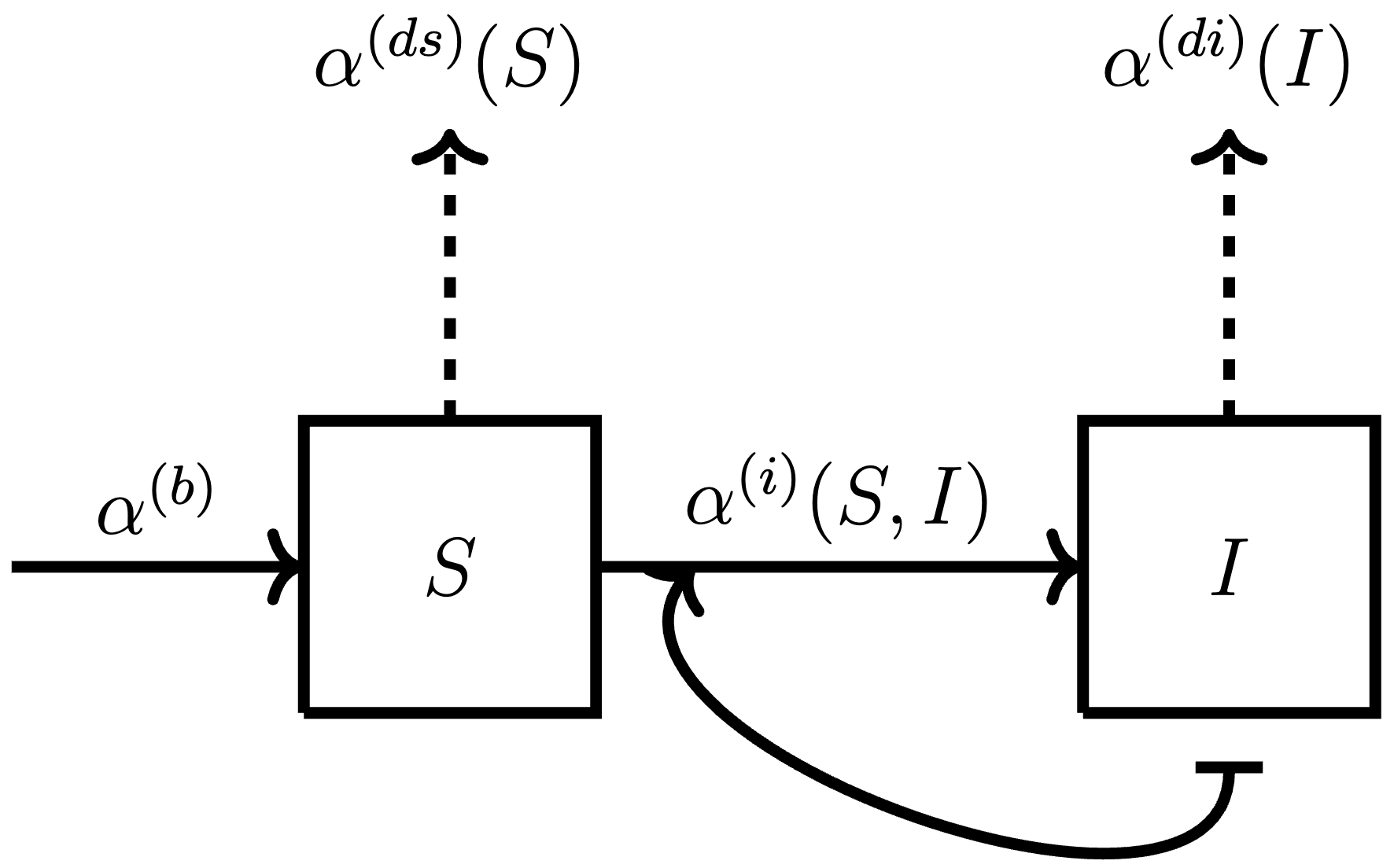
The simplest disease model, which underpins the core of most infectious disease models, describes the population-level dynamics of transmission between those susceptible to a disease and those capable of infecting others [FVHTSL12, MMP13]. To demonstrate the multiscale framework of this paper, we have opted to keep the disease model at the population scale as simple as possible. By assuming that individuals are removed at a constant rate in both susceptible and infectious states and that new individuals are introduced as susceptible, we adopt the well-known deterministic (Susceptible) – (Infectious) ODE model [AM92]:
| (1) | ||||
where and denote the number of susceptible and infectious individuals, respectively. The terms , , , and represent the rates of each of the events modelled within the system. These events are as follows: birth of susceptible, death of susceptible, death of infected and infection of susceptible individuals, respectively. Importantly, we use in general to represent rates and superscripts , , and to indicate specificity to each of the four event types. The constants and are, respectively, the rate at which new susceptible individuals enter the system, and the per capita death rate. The disease transmission coefficient is given by . The schematic diagram for this population-level model is shown in 1(a).
The SI model (1) has tractable fixed points . They are and . We shall refer to as the elimination state and as the endemic state. It is possible to show through linear stability and bifurcation analysis that a transcritical bifurcation occurs when . If , then the disease becomes endemic with being positive and stable whilst the disease elimination state is unstable. If , then has a negative infectious population and is therefore an irrelevant fixed point and is stable.
Model (1) encompasses fundamental features of most population scale infectious disease models. It, therefore, has been extensively studied as a cornerstone base case. We will extend this model to include multiscale behaviour in two steps:
-
1.
Use a stochastic simulation algorithm (SSA) at the population level. We note that as an ODE, the model only describes large continuous populations, and when populations or are small, the model is inappropriate. For example, if and , then may get arbitrary small. However, since is unstable, disease elimination is impossible. On the other hand, even if , elimination should be possible when is small. Because in reality a small number of infected individuals may, stochastically, recover or die before infecting anybody. Such an elimination event can be achieved by a stochastic simulation of model (1). For instance, a discrete and stochastic transition of individual to leads exactly to the elimination steady state . This is an absorbing state since small perturbations are not possible in the discrete stochastic (and thus realistic) scenario. We shall demonstrate in Subsection 2.1.2 how to extend model (1) into a stochastic simulation algorithm. Although for model (1), such conversion is widely understood, we shall highlight particular ideas useful for generating a multiscale model.
-
2.
Introduce a deterministic within-host model for individual infections. We note that one big assumption in model (1) is that the rates (or propensities) for population-level events to take place do not evolve during the inter-event time intervals. However, such an assumption may be an oversimplification in a real-world scenario. For example, each individual’s mortality rate at the population level can be related to its within-host pathogen load and immune responses [GMN14]. Moreover, a variety of experimental observations [EGB12, BWE+14] indicate that temporal changes in an infectious agent’s within-host viral load can be associated with its propensity to infect others. We, therefore, extend our model (1) by introducing a deterministic within-host model for the infectious population. In Subsection 2.1.2, we will highlight how time-dependent event propensities complicate the SSA algorithm. Then in Subsection 2.1.3, we will present a simple deterministic within-host model.
In Section 2.2, we combine the population-level SSA model and the within-host model to obtain a multiscale framework. The aim is to demonstrate an effective way to couple the deterministic changes of individual viral loads with stochastic simulations at the population level. Whilst we explore this with a simple dynamic model at both scales, the ideas in Section 2.2 are applicable to other multiscale models in a more general setting.
2.1.2 Converting population-level model into an SSA
The population-level model shown in (1) describes a system of deterministic interactions that govern the dynamics of an infectious disease. A key assumption behind the ODE formualtion is that populations are large and continuous, and hence noise can be ignored. The underlying discrete stochastic process of (1) is a continuous time Markov chain (CTMC), which describes the evolution of the discrete stochastic non-negative state . and , respectively, represent the number of susceptible and infectious individuals at time . They are piece-wise constant functions in time because the system remains in a constant state for an exponentially distributed amount of time until moving to the next state [All10]. Moreover, a CTMC has the Markovian property of being memory-less; its future state only depends on the current state of the system
[All17].
Consider an arbitrary time when and , we the define transition probabilities of the stochastic process from state to state by time as
| (2) | ||||
where is any positive interval of time. If the initial state of the system is known (or subject to a known distribution), then using the notation , the forward Kolmogorov equation to describe the stochastic system associated with the population-level ODE model (1) can be written as:
| (3) | ||||
Where possible, we shall reserve to represent ‘calendar time’; the time that has passed since the start of the population-level model.
The stochastic simulations of (3) – exact or approximate – are well-known in the literature and can be achieved in a number of ways. The simplest approach uses a small set time step , thus it is referred to as a time-driven algorithm. At each moment in time of a simulation, the current state of the system is known. Then, multiplying (3) by gives the update formula to the leading order:
| (4) | ||||
| (5) | ||||
| (6) | ||||
| (7) | ||||
| (8) |
where (with no superscript) is the sum of all (current) event rates. In stochastic contexts, the rates which we denote here using ’s are called propensities. We say that is the propensity for any event to occur. It follows that the probability of this event being birth, susceptible death, infectious death or infection is given by , , and respectively. The probability of any one of these events taking place in a given time step according to (4) is . For numerical simulation of the system, draw a uniform random number from 0 to 1. If it is less than , then is changed according to the event chosen from the weighted distribution of all possible events. It is straight-forward to see that this algorithm requires a very small for accuracy, which can lead to no events taking place in most time steps.
Two exact methods, the Gillespie algorithm (direct SSA) and Next Reaction Method (NRM) solve this problem by asking the question
| (9) |
Using (4), we can determine a probability density function in time for a state change if the current state is :
| (10) |
The use of the upper case emphasises that (10) is a distribution for a wait time from the current time (i.e. for a putative calendar time of ). The putative (event wait) time, can be drawn from . The use of the term ‘putative’ is common. This is because when is sampled, the event is scheduled for the calendar time . But this schedule may change if something changes the propenensity . In the direct SSA, all events are considered under a single propensity, so the putative time will always result in an event at . However, this is not the case for methods like the NRM.
The direct SSA and NRM take theoretically identical but practically different approaches to the question in (9). In the direct SSA, inverse transform sampling is used to draw an event time using the distribution (10):
| (11) |
where and is the cumulative distribution function associated with the density . After determining when an event occurs, the direct SSA then determines which event occurs based on the relative sizes of the probabilities (5)–(8). For example, the probability of a birth event (i.e. ) at calendar time is , similarly for the other events in proportion to their respective propensities. However for NRM, instead of determining when an event occurs followed by which event occurs, it reverses the order of these calculations by making use of two special properties of the exponential distribution (10). Firstly, given any sensible partition of the state propensity by event type where are the set of possible events (e.g., in this manuscript we have that ), (11) has the same probability density function as
| (12) |
where is independently sampled for each possible event and is the putative time associated with realising each event type. The most imminent event – the one with the smallest putative wait time – is the event which is chosen to propagate the simulation forward. Importantly, because of the exponential distribution (10), the event corresponding to this most imminent time has a probability that matches the probability of the event determined in the direct SSA. Therefore in the NRM, putative times for event types () are drawn and stored as an array. The minimum event putative time (, ) is then determined to be the ‘next reaction’ and the state is updated according to the event associated with this putative time. Interestingly, the second property of the exponential distribution (10) then allows for the NRM to be efficient. Instead of throwing away and resampling (rescheduling) all putative times for all events , the times are kept and updated by first subtracting (. We use the dash notation to indicate that a wait time has been updated to a new wait time due to the moving forward of time. Then the state is changed based on the event , which subsequently changes many of the event propensities. Because each of the putative times have been initially sampled from exponential distributions, their updated values are conditioned on , which are also exponentially distributed random numbers with propensity (the lack of markings here highlighting that this is the propensity prior to any state change due to event ) and there is no need to resample the putative event times which are computationally expensive to sample. An updated putative time needs to be generated for the event . However it is clear from the sampling equation (11) that all other events just need to be scaled after the event :
| (13) |
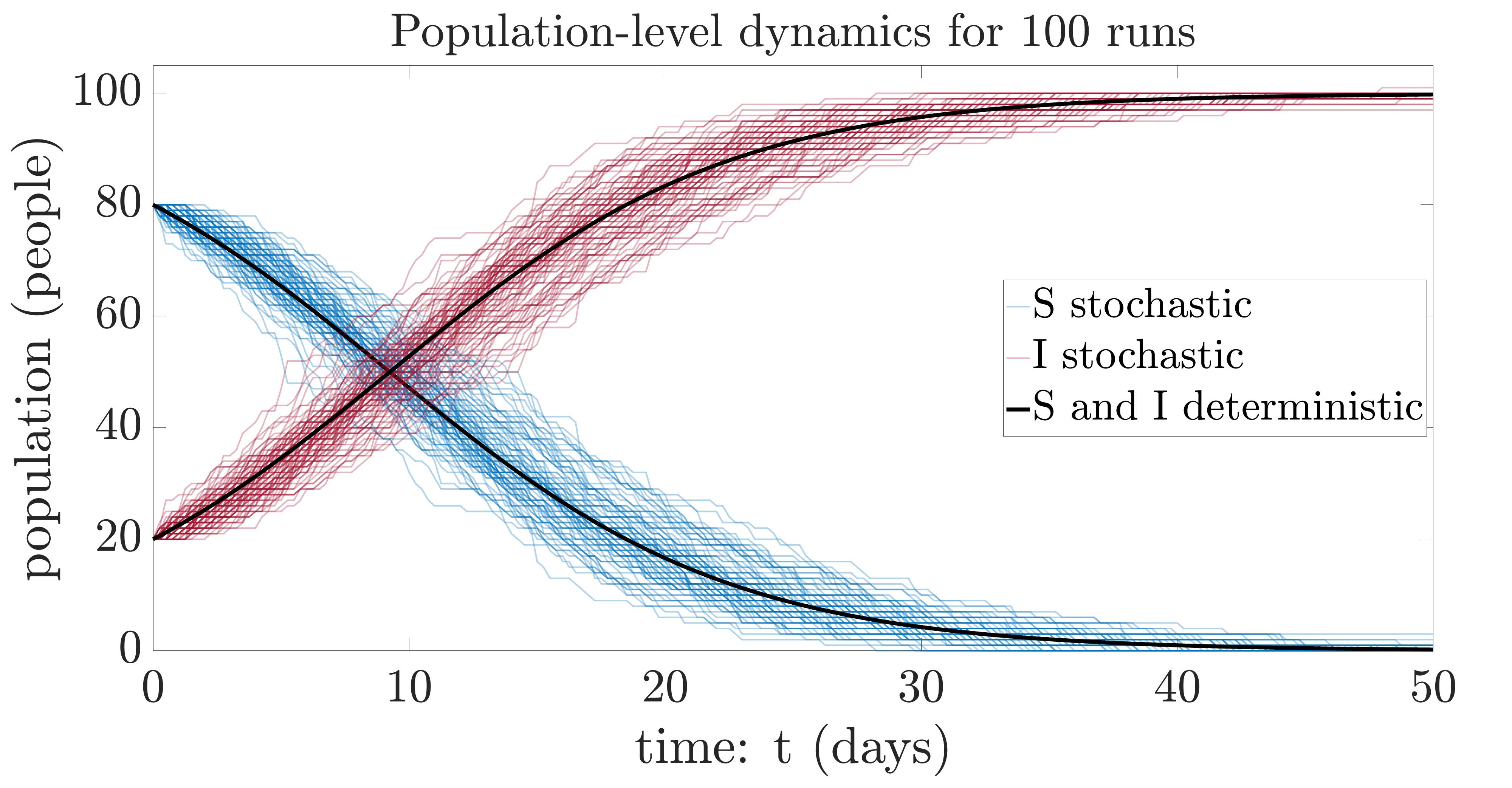
where the bar indicates that the quantity has been updated for the change of current time from to (the dashed notation), and also updated for the change of state/propensity associated with event from the time to the new putative calendar event time of . After all calculations are done to update the state and putative times for the event , becomes the current time and the new state becomes the current state (so bars and dashes are subsequently dropped to be used to denote the updates for the next event). Using the Gillespie direct SSA or the NRM, an exact stochastic simulation of the model is possible. In 1(b) we show simulations of this algorithm against the deterministic ODE model (1).
The purpose of discussing these known stochastic methods in detail here is to highlight the importance of the Markovian property in the population-level system. That is, event times are exponentially distributed (10) and do not depend on history or time explicitly between events (when the state of the system is constant). One nontrivial issue, which we shall address in detail, can arise if the state of the system is changing in time between events. In multiscale (for example within-host and population-level coupled) models, population-level propensities can depend on within-host dynamics, and thus change with time between population-level state changes. The obvious solution here is to attempt to adapt the within-host model into the SSA and generate putative times for all events (including those within each infectious individual). In this respect, all events, irrespective of whether they are population-level or within-host level would be modelled exactly. However, it is completely infeasible to do this since: 1) there may be a large number of infectious individuals; 2) each individual will have their own SSA; and 3) there may be an extremely large number of within-host events simulated before a single population-level model event (the multiscale problem). Instead, because the within-host dynamics are associated with much smaller timescales compared to the population-level dynamics, it becomes crucial to develop an appropriate method for running an SSA at the population level subject to deterministic and smooth time-varying propensities (in our case as a result of changing viral load of each individual). We are therefore faced with the following two challenges: 1) time varying propensities: propensities that may change with time between discrete event times; and 2) the individuality problem: temporal change in propensities may be complex due to individual contributions and subject to historical events (for example the previous times when individuals become infected). The time varying propensity problem has known solutions and can be solved exactly as we shall demonstrate. Of course, sometimes the additional work required to deal with this problem exactly is not considered to be worth the effort and approximate algorithms, such as -leaping, are used (appropriate when the relative change in propensity between events is sufficiently small and therefore approximated to be constant) [Gil01]. The individuality problem is a much harder problem. This is unsurprising since more detail in SSA simulations and, indeed, any model, will always increase computational demands. To overcome these two challenges, we introduce in the next section a simple within-host model to use as a test problem and we assume that, once infected, all individuals deterministically trace solutions of this model. This means that what separates individuals is the initial time of infection only.
2.1.3 Within-host model
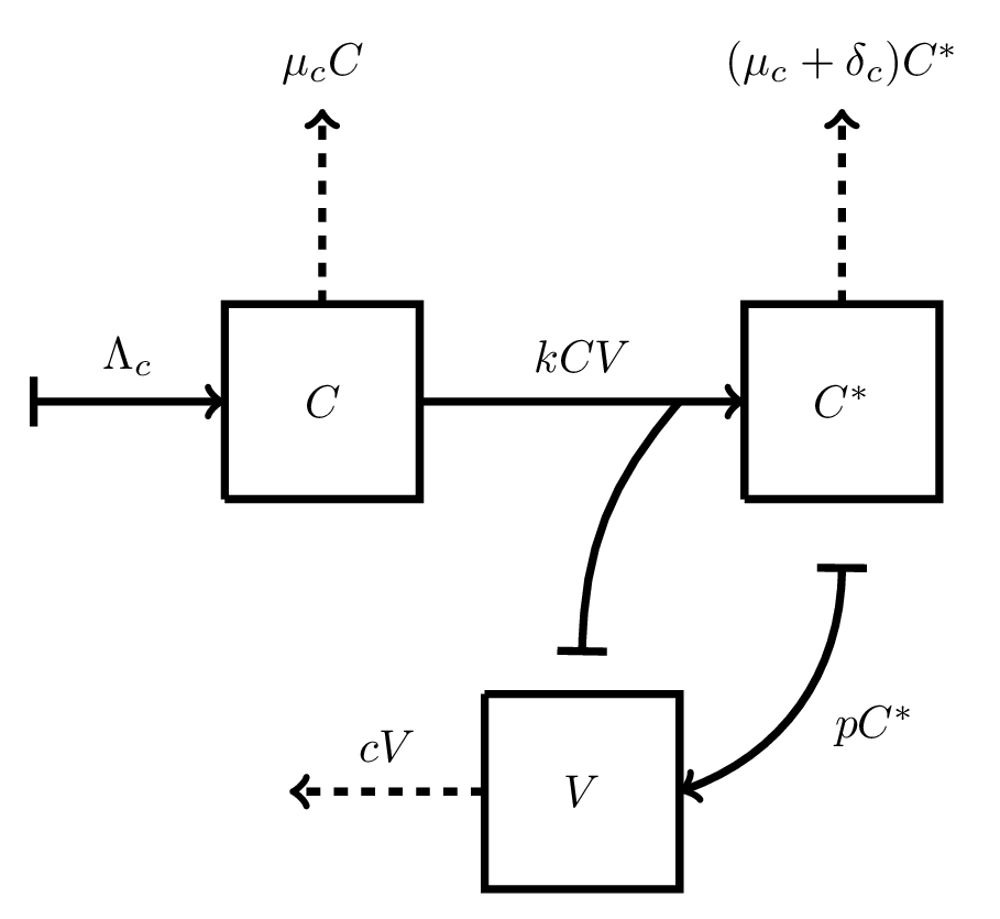
In general, a within-host model describes viral dynamics and immune responses at the cellular level in one single host [FVHTSL12, MMP13]. By assuming that the within-host dynamics can be controlled by target cell limitation only, we choose to rely on an extension of the deterministic target cell-limited model as shown in (14):
| (14) | ||||
The independent variable in the context of the within-host model denotes the age of infection of this infectious host (i.e. the time since their initial infection). One should keep in mind that is different from , the population-level calendar time. The numbers of uninfected cells, infected cells, and virus particles are denoted by , , and , respectively. We assume that the rate at which new target cells are created is given by . The virus is produced at a rate of while is its clearance rate, and the infection coefficient of healthy cells is given by . The constants and denote, respectively, the mortality rate of the cells and the additional death rate for infectious cells. The schematic diagram for this within-host model is shown in 2(a).
2.1.4 Model coupling
With the specific population-level and within-host sub-models discussed in Subsection 2.1.1 and Subsection 2.1.3, respectively, we can now construct a multiscale model by linking these separate sub-systems. Theoretically, this coupling process can be facilitated through identifying possible parameters and variables in one sub-system that affect the dynamics of the other and consistently formulating a feedback across sub-models. A common approach to accomplish this is by expressing that set of parameters or variables in one sub-model as functions of those in the other [GMN14]. In this Subsection, we will develop a test multiscale model that links the population-level transmission coefficient to the within-host viral load. It is important to note that, to illustrate the simulation methodology, the model coupling presented below represents just one method to connect these scales.
Although a variety of experimental observations [EGB12, BWE+14] indicate that population-level disease transmission is often associated with the infectious agent’s within-host pathogen load, the specific functional form between these quantities is still uncertain [HR15]. For simplicity, we assume that each agent’s transmission coefficient is a linear function of the viral load associated with that agent, with proportional constant , which takes the unit . Whilst we have chosen a linear relationship between the viral load and the agent transmission coefficient, the nature of relationship does not affect at all the applicability of this method. We recall that is the viral load of an individual with age of infection . We shall assume that all infectious individuals within-host dynamics are governed by the same deterministic model (14). Thus, for a specific infectious individual , the corresponding transmission coefficient at time is
| (15) |
where . In (15), is the calendar time associated with the initial infection of individual and is the age of the infection in that individual. Note that the individuality of is encapsulated only in the initial infection time . We further assume that within-host dynamics is independent from the population-level dynamics (and can be solved numerically once at the start of the simulation). The function is assumed to be zero prior to infection (), so as to account for the agent being susceptible (noninfectious).
A more complicated model can include further stochasticity in the parameters of the within-host model (14) among individuals. In this case, the appropriate change to the population-level model simply requires noting that is different for each . However, introducing more individuality into the model substantially complicates the computational requirements. Therefore, for a level of novel tractability of the problem, we shall look only at the case where the within-host model is deterministic and the dynamics are the same for each individual post-infection.
Simulating the multiscale coupled model involves replacing the transmission term in (1) with a non-Markovian (explicitly time-dependent) one, which is derived from the sum of the total viral load in the infectious population:
| (16) |
Since the propensity now depends explicitly on time, the previously mentioned algorithms in Subsection 2.1.2 need to be updated. Furthermore, it is important to note that this function of time is complex as the infection times are stochastic.
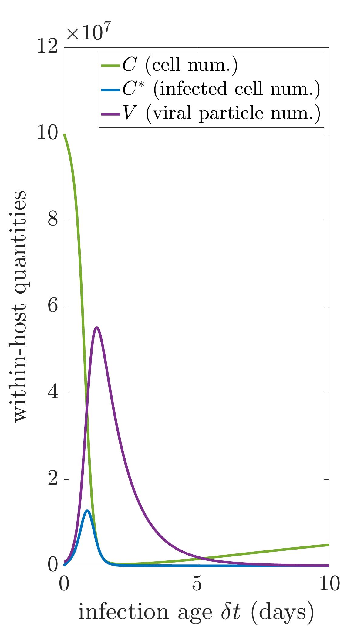
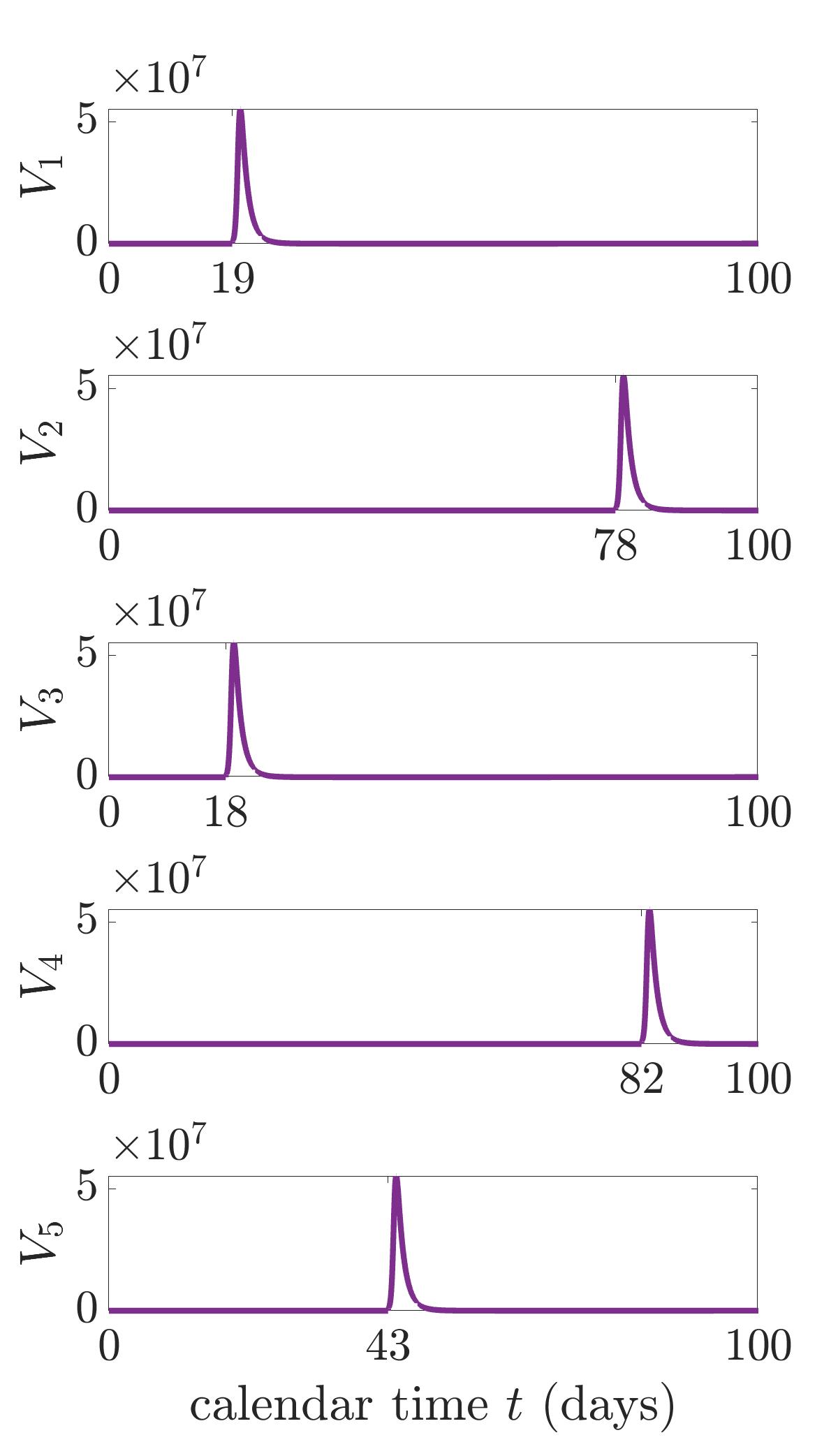
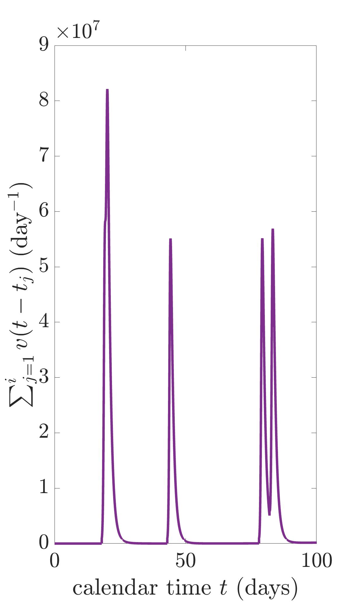
Diagrammatically, the integration of the within-host model is shown in Figure 2. The schematic diagram for the within-host model is presented in Figure 2(a). In Figure 2(b) we solve this model to determine the within-host viral load for an individual as a function of its age of infection . In Figure 2(c) we use the known viral load from the solution of the within-host model and position the starting time day to be at the calendar times for each infected individual (of which we plot 5 sample individuals becoming infected at various times) in the population-scale SSA. Finally, we note that what drives the SSA is the total infectious propensity as computed by (16), the sum of all individual transmission rates in the system multiplied by the susceptible population and presented in Figure 2(d).
2.2 Multiscale model simulation
The within-host model (14) can be solved numerically to give . The multiscale stochastic model can therefore be written in the same manner as (3) in Subsection 2.1.2, but noting the change in transmission coefficient as shown in (16). Probabilities for updating the simulation from known state from (4)-(8) in the multiscale case at time is conditional on the set of times in the past individuals firstly became infectious. That is, by denoting as the probability of being in state conditional on known infection times :
| (17) | ||||
| (18) | ||||
| (19) | ||||
| (20) | ||||
| (21) |
Applying the NRM in the case of the time dependent total propensity , putative times for birth and deaths can still be found in the standard way as their Markovian property still holds. However, drawing a putative time for the next infection event requires sampling from a distribution with a time dependent rate. The derivation of such putative time is to sample the time for a particular event conditional on the state remaining unchanged. According to (21), the probability of an infection in time interval is . Let be the probability that no infection occurs in the first time steps from . We have
where . We notice that
| (22) |
We define the survival distribution function as the probability that no infections have occurred in time interval in the limit . By setting and taking the limit , we find that
Therefore, the survival distribution function as well as its complement, the cumulative distribution function (CDF), associated with the putative time for infection are
| (23) |
where
| (24) |
Note for notational simplicity, . By storing numerically in a look-up table rather than , it is therefore possible to quickly obtain .
A sample of the putative time for an infection can be generated by sampling a random number and solving for , where is the current calendar time. This is complicated because the exponent in as shown in (23) is a nontrivial function which depends on the stochastic history of infections among the infectious population. Furthermore, even if efficient sampling from the CDF in (23) is solved, is only a putative time for infection at current calendar time ; once the within-host as well as the population-level states change when time forwards and when any event occurs, a new putative time would need to be sampled. In Subsection 2.2.1, we will firstly outline an approximate computational algorithm that uses discrete time steps and equations (17)-(21) to simulate the multiscale scenario. Since the algorithm propagates forward in time using fixed time steps, they are usually called ‘time-driven’ algorithms. This is in contrast to the direct SSA or NRM approaches which propagate forward in time by the occurrence of events; aptly named ‘event-driven’ approaches. We will then outline our main result in Subsection 2.2.2; an exact NRM method where is efficiently sampled using the CDF presented in (23).
2.2.1 Approximate time-driven simulation
The time-driven algorithm we will present in this subsection is rather simple but is only approximate. It uses a predetermined fixed small time step with brute force to simulate events using (17)-(21). Reducing the size of allows for control over the level of accuracy but at the cost of efficiency. We shall use this algorithm to compare with the main algorithm of this paper in Subsection 2.2.2. The pseudocode for this algorithm is shown in Algorithm 1. The algorithm is a simple extension of the time-driven algorithm previously discussed in Subsection 2.1.2.
2.2.2 Accurate multiscale simulation
In NRM, the event with the minimum putative time is selected and the state is updated to corresponding to the change caused by that event. After changing the state, the time is first updated and then the putative time for the event that occurred is resampled. For all other events, the putative time is updated to reflect the progression of time and then rescaled to reflect any change in propensity as a result of the transition to . In this section, we present a NRM algorithm for simulating non-Markovian disease transmission models of the type explored in this manuscript. We focus on how putative times corresponding to within-host infections are computed, resampled, and rescaled to be used in the general next reaction method framework.
To find we could attempt to solve where , where is defined in (23). However, instead of finding a putative time for the next infection, we note that infected individuals are unique in this model (at least when it comes to infecting others) and therefore it is more tractable to subdivide infection events by the individual who is responsible for the infection; and find a putative infection time for each infected individual as . We shall then use the minimum of these putative times by the NRM to determine . In fact, going further than this we determine the update time . Using this method of treating each individual infected person separately, we also have the capability of storing data on who is responsible for distributing the disease for later analysis without any further calculation.
We are permitted to (and indeed benefited by) applying the NRM in this way because
| (25) |
We denote the survival probability for an infection by infectious individual to be
| (26) |
and similarly . Note that ; denotes the age of infection; is defined in (15). Let . The NRM asserts that and have the same distribution, which can easily be seen by (23)
Note that because each of the putative times are independently sampled, the survival distribution function for the next infection time (23) is the product of that for each infectious person (26). Therefore, by breaking down the infection event by infectious individual, we do not have to compile the information about the distribution of viral loads in the population to calculate a putative time for an infection.
In the NRM, when , the ‘next event’ is infection by the th infected individual. For this individual, the next infection will need to be resampled. For all other putative times, where , the NRM describes a rescaling of the putative time instead of resampling for efficiency. We describe both resamplng and rescaling next in detail.
Resampling
Drawing a putative time from the survival distribution function (26) for each infected individual is achieved by first sampling and using a look up table to solve for where . To achieve this, it makes sense when looking at (26) to focus on the variable instead of since this allows us to tabulate a function that is independent of as follows. Using (26) and recalling that ,
| (27) |
That is, the value of gives the putative increase in the function (which is independent of ) from the current time to the time of the infection. We therefore track four values for each infected individual: (1) the current value of the individuals infection time , (2) the current putative time until the individual next infects a susceptible , (3) the current value of , and
(4) the current putative change the value of when the individual next infects . It is the later putative variable (not the putative time ) which can easily be sampled. However, as time moves forward and infection time needs updating, this has to be done in the time domain by shifting .
Resampling should be done if .
In the case of resampling, time should be first updated to the new infection time
| (28) |
where the bar notation indicates the ‘new’ value of the variable. The update step also allows for the calculation of the new , that is by the lookup table for the function .
Second, after the change of state to a new putative is sampled for the individual; by (27) reflecting the new . Finally, it is possible to determine the new putative time . This is done simply by knowing , and and using the lookup table to invert the function :
| (29) |
A schematic showing how is resampled is presented in Figure 3. Here we show how the update in time (green) is to the putative time for the individual () and the time is first updated. By the green dashed line, it can be seen how the new infection time for the th individual, , corresponds to the new value for this infectious individual. From here, the resample step is given in red. A putative future increment in () is computed and then (by the red dashed line) a new putative time until next infection is determined.
Rescaling
If naively, it is possible to simply update , , and using the resampling method. This is however costly because it involves generating a new random number . Instead, a rescaling is possible. But unlike the classical NRM where this rescaling is done to , it is necessary to instead rescale in . To be clear, and are calculated as before. We note however that since , there is a portion of time between and for which the propensity is changed due to the change of state from its original value . This corresponds to the interval in of width
| (30) |
It is possible to reuse and rescale to generate such that it has the same probability density as it would if it were resampled using . This is achieved by using the rescaling
| (31) |
This reuse of the random number is possible since
| (32) |
where and is the wait time from instead of , indicating an update in the calendar time. Of course, the probability of finding the updated putative time assumes that the value of is not changed to at the time . We therefore note that can be generated with its correct probability by . The true updated should instead use the correct (new) susceptible population . That is, . The value of the updated putative time is then calculated in the standard way using (29).
A schematic showing how is updated and then rescaled after each event (that takes place at the infection time of in the schematic) is presented in Figure 4. Here we show how the update in time to the next putative time (green). The new current infection time for this individual is then related to the new parameter for this individual. The remaining parameter separating the new and the old putative parameter is indicated. In red, this putative parameter is then scaled to give a new putative value of which in turn is used to generate the putative time using a look-up table.
2.2.3 Implementation of accurate multiscale simulation
To simulate the within-host and population-level integrated model, we take the framework of a typical population-level Gillespie style SSA. The algorithm updates from event to event via a generalised next-reaction method (NRM) by storing all putative times for each unique event and implementing the event corresponding to the most imminent. Putative times for all Markovian events (in our case events , , and ) are drawn in the same way as described in Subsection 2.1.2. However, times for the non-Markovian events (in our case ) need to be treated differently. We shall store in a complete list of putative times for all Markovian events. In particular, . Furthermore, for each infected individual we also keep track of four pieces of information , , and . Whilst it is the case that elements in are related to elements in in the same way as elements of to those of , by the function , we find it convenient to store and track all four numbers for each infected individual.
It is necessary to begin by having a numerical solution for the within-host model and, together with (24), store in a table. The table is stored with a discretisation of given by . Specifically, we store , , , and so on. Importantly, whilst this algorithm is accurate, the source of error is associated with the resolution of this table, so should be small. If is too small, however, using the look-up table becomes an expensive operation. From here on, we shall simply use the operators and to reference using this look-up table, and, rounding to the closest stored value, if necessary. We use these operators liberally so that when they are applied to a vector of values, it is implied that the look-up table is used element by element, and therefore a vector of output values is being represented.
We begin by initialising all population compartments (, ). For each infected individual , it is necessary to determine an initial calendar time of infection and use this time to initialise . We use the look-up table to initialise . Next we initialise all putative times. We initialise by finding respective propensities for each element and sampling putative times using (11). We then initialise for each element by using (27) and then use the look-up table to initialise . The algorithm propagates forward by finding the most imminent event time . After finding the event, time is updated and then the event is implemented (changing the compartments and deleting or initialising elements of , , and , respectively) and then its putative time is re-sampled whilst all other affected putative times should be re-scaled (either using (13) if it is a Markovian event or (31) if it is a non-Markovian - infection - event). In particular, re-sampling and re-scaling of the non-Markovian infection events are described in Subsection 2.2.2 and involve updating respective elements of , then followed by and then . The algorithm then propagates until some pre-determined final time. As shorthand, we shall denote as the collection of vectors that store information about each infected individual.
3 Results
| Initial conditions | Values for |
|---|---|
| health cells | |
| infected cells | |
| viral particles | |
| Parameters | Values |
| Parameters | Values |
|---|---|
In this section, we aim to validate the accuracy of our novel algorithm (Algorithm 2) compared to an equivalent approximate time-driven method (Algorithm 1). In the approximate Algorithm 1, the calendar time is discretised with finite fixed time step , while in our novel Algorithm 2, time discretisation is limited to the resolution of tabulated associated with the within-host model. We shall denote this later discretisation as and note that it is possible to make this very small whilst incurring only the cost of reduced efficiency in using the table. It’s worth noting that whilst represents a coarse-graining of the within-host model dynamics, the calendar discretisation represents a course-graining in within-host and population scale models. That is, it is possible to miss intra-timestep population scale events with Algorithm 1 but not with Algorithm 2. However, if , Algorithm 1 is expected to yield accurate results. Numerically, the which guarantees the accuracy of the approximate algorithm is chosen such that
where . For the initial condition people, we have day based on parameter values and within-host initial conditions shown in Tables 1–2. To assess the accuracy of our novel algorithm, we contrast consistent discretisation between the two algorithms and vary this discretisation geometrically over 131 points. Specifically, days. In Figure 5, we visualise the course-graining of the within-host viral load as a result of using day, day, and day under the assumption that within-host virus dynamics occur as a result of specific model parameters presented in Table 1. We include in this figure the discretisation for both Algorithm 1 and 2. The reason for this is subtle. Sampled viral loads under Algorithm 2 are tabulated starting at day. On the other hand, we assume that in Algorithm 1 that an infection begins on a time step and thus we sample halfway between time steps as the best approximation of the viral load on this time interval. The difference in implied numerical viral load when day is clear in Figure 5. We refer to the error associated with the discretisation of the within-host model as ‘resolution error’. We are not deterred from labelling Algorithm 2 as being an ‘exact’ algorithm since the algorithm is, at least in principle, exact if the continuous function is known in the same sense that the Gillespie algorithm is exact despite the fact that there may be numerical error in the propensities.
We designate the approximate time-driven algorithm with day as the ‘Golden Standard’ (GS), against which we will compare our novel algorithm. Figure 6 compares the population-level dynamics of the approximate Algorithm 1 and our novel Algorithm 2 with the GS, given day. The ‘diamond’ markers in Figure 5 visualise how we extract the within-host dynamics based on such resolution. One can observe that as long as the within-host dynamics is approximated at a satisfactory level, or equivalently the ‘resolution error’ is not surprisingly dominant, our novel algorithm converges to the GS and is indeed accurate. In contrast, the dynamics of the approximate time-driven algorithm are notably slower than those of the GS. This is because the time-driven Algorithm 1 suffers from inaccurate approximation of probabilities for state changes at the population-scale which are not present in Algorithm 2.
We now quantify the accuracy comparison between the two algorithms. To quantify the error produced by the algorithm, we determine the calendar time in the test model at which the infectious and susceptible populations are equal . We then subtract this time from the time in the GS simulation and then divide the result by the GS time to get a relative error. This error is plotted in Figure 7 against the choice of . The solid curves show the error associated with Algorithm 2 whilst dotted curves present the error associated with Algorithm 1. The different colours indicate the effect of population size. In particular we use the different initial conditions: , , , and people, respectively. The coloured ‘dot’ markers indicate the largest time step possible in Algorithm 1 in order that the error is kept below , for comparison the coloured ‘asterisk’ markers indicate the same limitation on in Algorithm 2. It can be observed that as we scale up the population, decreases linearly in the log scale of Figure 7, whereas is relatively unaffected by population size and good accuracy can be achieved with relatively coarse discretisations of around day. The error observed for Algorithm 2 is due solely to ‘resolution error’ which is a discretisation of within-host model but will not affect the population-scale, as previously explained.


4 Discussion
When simulating a population-scale model of the spread of a disease, it is not uncommon to see the implementation of autonomy (memorylessness) in the model. This is the case with ODE and also Gillespie-type stochastic simulations. In the case of small populations, where the outcome of an epidemic may hinge on the infections of one or two infected individuals, these memoryless models do not factor in the progress the individuals are making with the disease. To track an individual’s viral load, a within-host model is required to be coupled to the population-scale model. We have shown that the introduction of a within-host model for each individual can be achieved with extremely small time steps. However, such a time-driven algorithm becomes inaccurate (Figures 6–7) if the fixed time step is no longer small enough. It is important that the time step chosen is much smaller than the natural rate of change of viral load for an infected individual. Additionally, since working with predefined finite time steps, it is important to keep the time step much smaller than the inverse of the rate of infection and therefore the time step should depend on the unknown future population-level and the overall within-host level dynamics, which is almost impossible to estimate. This is because it is assumed that the probability for an event to occur in any given time step should be small. Whilst Tau-leaping style approaches might also be useful, they too require some consideration for the rate at which events are occurring in order to retain sufficiently high accuracy. In this paper, we have sidestepped this challenge and developed a novel stochastic algorithm (Algorithm 2) for multiscale systems which incorporates a within-host viral load dynamic into the infection rates of individuals embedded in a population-scale model of an infectious disease. The key strength of our algorithm lies in its accuracy and generality. Specifically, event times are simulated in a similar way to the Gillespie algorithm but taking into consideration the explicit time dependence in individual viral loads. We conclude from Section 3 that as long as the within-host data are extracted at a sensible resolution, the simulated results will always be accurate using our approach. Additionally, while we have introduced the concepts of this novel approach using simple within-host and population-level models, our algorithm can be applied to similar compartmental models at both levels. We thus conclude that our accurate Algorithm 2 can be broadly applied across the field of multiscale infectious disease modelling.
The primary contribution of this study lies in the development of a novel algorithm and the demonstration of its accuracy. The evaluation of its efficiency is reserved for future investigation. This novel algorithm can also be extended in several directions. For instance, we can explore scenarios where the whole population still shares a single within-host system, but it is no longer deterministic and includes noise. Alternatively, given a single deterministic within-host system, we can investigate situations where different infectious individuals have varying within-host time scales. Moreover, our algorithm can be expanded to accommodate heterogeneous populations, such as those with age structures, where each sub-population shares a single deterministic within-host system. In this case, one can simply create different lookup tables (see (24)) that tabulate different within-host dynamics for each sub-population.
Our work also holds broader implications and significance in real-world scenarios. Until now, while considerable effort has been dedicated to nesting the within-host system into the population-level system in multiscale modelling of infectious diseases [TAKT23, MTSM15, MAD08], the reverse direction has not been fully explored [FVHTSL12]. The novel accurate Algorithm 2 we have developed can serve as an ideal tool for generating and harvesting global within-host information averaged across the entire population. In this sense, one may uncover potential relationships between these two subsystems and, consequently, nest the population-level system back into the within-host one. The advantage of doing so lies in the fact that, after coarse-graining, a single set of ODEs can be achieved, incorporating both population-level and averaged global within-host dynamics. As a result, it would be much more efficient to test, refine, and calibrate the simple yet comprehensive coarse-grained ODE model to real-life data. Parameter inference would also be more realistic, enabling predictions and the formulation of policies to slow down disease transmission.
5 Data accessibility
6 Acknowledgements
J.A. Flegg’s research is supported by the Australian Research Council (DP200100747, FT210100034) and the National Health and Medical Research Council (APP2019093). Y.Yin is funded by the Engineering and Physical Sciences Research Council (EP/W524311/1). This research was supported by The University of Melbourne’s Research Computing Services and the Petascale Campus Initiative. All authors declare that the research was conducted in the absence of any commercial or financial relationships that could be construed as a potential conflict of interest.
References
- [All10] Linda JS Allen. An introduction to stochastic processes with applications to biology. CRC Press, 2010.
- [All17] Linda JS Allen. A primer on stochastic epidemic models: Formulation, numerical simulation, and analysis. Infectious Disease Modelling, 2(2):128–142, 2017.
- [AM92] Roy M Anderson and Robert M May. Infectious diseases of humans: dynamics and control. Oxford university press, 1992.
- [ANHV18] Alexis Erich S Almocera, Van Kinh Nguyen, and Esteban A Hernandez-Vargas. Multiscale model within-host and between-host for viral infectious diseases. Journal of Mathematical Biology, 77(4):1035–1057, 2018.
- [BWE+14] Nello Blaser, Celina Wettstein, Janne Estill, Luisa Salazar Vizcaya, Gilles Wandeler, Matthias Egger, and Olivia Keiser. Impact of viral load and the duration of primary infection on HIV transmission: systematic review and meta-analysis. AIDS (London, England), 28(7):1021, 2014.
- [CGP06] Yang Cao, Daniel T Gillespie, and Linda R Petzold. Efficient step size selection for the tau-leaping simulation method. The Journal of chemical physics, 124(4):044109, 2006.
- [DHB12] Odo Diekmann, Hans Heesterbeek, and Tom Britton. Mathematical tools for understanding infectious disease dynamics. Princeton University Press, 2012.
- [EGB12] Kathryn M Edenborough, Brad P Gilbertson, and Lorena E Brown. A mouse model for the study of contact-dependent transmission of influenza A virus and the factors that govern transmissibility. Journal of Virology, 86(23):12544–12551, 2012.
- [FVHTSL12] Zhilan Feng, Jorge Velasco-Hernandez, Brenda Tapia-Santos, and Maria Conceição A Leite. A model for coupling within-host and between-host dynamics in an infectious disease. Nonlinear Dynamics, 68(3):401–411, 2012.
- [Gar18] Winston Garira. A primer on multiscale modelling of infectious disease systems. Infectious Disease Modelling, 3:176–191, 2018.
- [Gar20] Winston Garira. The research and development process for multiscale models of infectious disease systems. PLoS Computational Biology, 16(4):e1007734, 2020.
- [GB00] Michael A Gibson and Jehoshua Bruck. Efficient exact stochastic simulation of chemical systems with many species and many channels. The journal of physical chemistry A, 104(9):1876–1889, 2000.
- [Gil77] Daniel T Gillespie. Exact stochastic simulation of coupled chemical reactions. The Journal of Physical Chemistry, 81(25):2340–2361, 1977.
- [Gil01] Daniel T Gillespie. Approximate accelerated stochastic simulation of chemically reacting systems. The Journal of Chemical Physics, 115(4):1716–1733, 2001.
- [GJG+20] Rebecca B Garabed, Anna Jolles, Winston Garira, Cristina Lanzas, Juan Gutierrez, and Grzegorz Rempala. Multi-scale dynamics of infectious diseases, 2020.
- [GM19] Winston Garira and Dephney Mathebula. A coupled multiscale model to guide malaria control and elimination. Journal of Theoretical Biology, 475:34–59, 2019.
- [GMN14] Winston Garira, Dephney Mathebula, and Rendani Netshikweta. A mathematical modelling framework for linked within-host and between-host dynamics for infections with free-living pathogens in the environment. Mathematical Biosciences, 256:58–78, 2014.
- [HAA+15] Hans Heesterbeek, Roy M Anderson, Viggo Andreasen, Shweta Bansal, Daniela De Angelis, Chris Dye, Ken TD Eames, W John Edmunds, Simon DW Frost, Sebastian Funk, et al. Modeling infectious disease dynamics in the complex landscape of global health. Science, 347(6227), 2015.
- [HR15] Andreas Handel and Pejman Rohani. Crossing the scale from within-host infection dynamics to between-host transmission fitness: a discussion of current assumptions and knowledge. Philosophical Transactions of the Royal Society B: Biological Sciences, 370(1675):20140302, 2015.
- [KR08] MJ Keeling and P Rohani. Modeling infectious diseases in humans and animals. 837 princeton university press, 2008.
- [MAD08] Nicole Mideo, Samuel Alizon, and Troy Day. Linking within- and between-host dynamics in the evolutionary epidemiology of infectious diseases. Trends in Ecology & Evolution, 23(9):511–517, 2008.
- [MMP13] Lisa N Murillo, Michael S Murillo, and Alan S Perelson. Towards multiscale modeling of influenza infection. Journal of Theoretical Biology, 332:267–290, 2013.
- [MTSM15] Maia Martcheva, Necibe Tuncer, and Colette St Mary. Coupling within-host and between-host infectious diseases models. Biomath, 4(2):ID–1510091, 2015.
- [SRL05] Davey M Smith, Douglas D Richman, and Susan J Little. HIV superinfection. Journal of Infectious Diseases, 192(3):438–444, 2005.
- [TAKT23] Yuichi Tatsukawa, Md Rajib Arefin, Kazuki Kuga, and Jun Tanimoto. An agent-based nested model integrating within-host and between-host mechanisms to predict an epidemic. PloS One, 18(12):e0295954, 2023.
- [Tom01] Masaru Tomita. Whole-cell simulation: a grand challenge of the 21st century. TRENDS in Biotechnology, 19(6):205–210, 2001.