Gradient Descent on Logistic Regression with Non-Separable Data and Large Step Sizes

Abstract

We study gradient descent (GD) dynamics on logistic regression problems with large, constant step sizes. For linearly-separable data, it is known that GD converges to the minimizer with arbitrarily large step sizes, a property which no longer holds when the problem is not separable. In fact, the behaviour can be much more complex — a sequence of period-doubling bifurcations begins at the critical step size $2/\lambda$, where $\lambda$ is the largest eigenvalue of the Hessian at the solution. Using a smaller-than-critical step size guarantees convergence if initialized nearby the solution: but does this suffice globally? In one dimension, we show that a step size less than $1/\lambda$ suffices for global convergence. However, for all step sizes between $1/\lambda$ and the critical step size $2/\lambda$, one can construct a dataset such that GD converges to a stable cycle. In higher dimensions, this is actually possible even for step sizes less than $1/\lambda$. Our results show that although local convergence is guaranteed for all step sizes less than the critical step size, global convergence is not, and GD may instead converge to a cycle depending on the initialization.

1 Introduction

Logistic regression is one of the most fundamental methods for binary classification. Despite being a linear model, logistic regression and its multi-class generalization play a significant role in deep learning, appearing in tasks like model fine-tuning. Given features $x_{i}\in\mathbb{R}^{d}$ and binary labels $y_{i}=1$ or $-1$, the goal is to find a linear classifier $w^{*}\in\mathbb{R}^{d}$ by solving the following optimization problem

$$w^{*}\in\operatorname*{arg\,min}_{w\in\mathbb{R}^{d}}{\mathcal{L}}(w)\coloneqq\frac{1}{n}\sum_{i=1}^{n}\log\left(1+\exp(-y_{i}w^{\mathsf{\scriptscriptstyle T}}x_{i})\right).$$ (1)

Since $w^{*}$ generally does not admit a closed-form expression, iterative methods such as Gradient Descent (GD) are typically used. GD solves this problem by iterating

$$w_{t+1}\leftarrow w_{t}-\eta_{t}\nabla\mathcal{L}(w_{t}),$$ (2)

where $\eta_{t}$ is the step size. As ${\mathcal{L}}$ is convex and $L$-smooth, classical optimization theory guarantees that a constant step size $\eta_{t}=\eta<2/L$ is sufficient for GD to converge to $w^{*}$ (Nesterov, 2018).

Recently, there has been a line of interesting discoveries on the behavior of GD, particularly for logistic regression. For linearly-separable data, Soudry et al. (2018) showed that GD with the $2/L$ step size converges to the maximum-margin separator. In fact, this holds true for any step size $\eta>0$ (Wu et al., 2023). An intuitive explanation is that if the data is separable, $w^{*}$ is attained at infinity, and so $w_{t}$ converges in the maximum-margin direction but diverges in magnitude. This result shows that the $2/L$ condition on the step size is unnecessarily conservative for logistic regression.

If the data is not linearly-separable, the objective is strictly convex as long as the features have full-rank, thus the unique minimizer $w^{*}$ is finite. For this reason, one can not expect convergence under an arbitrarily large step size: indeed, classical dynamical systems theory (Strogatz, 2018; Sayama, 2015) shows that $w^{*}$ becomes unstable when the step size $\eta>2/\lambda$, where $\lambda$ is the largest eigenvalue of the Hessian of $\mathcal{L}$ at $w^{*}$. A natural question to ask is whether this is the only barrier in the non-separable case: can we still guarantee convergence, as in the separable setting, using a “large” step size $\eta$ between $2/L$ and the “critical” step size of $2/\lambda$? And what happens at even larger $\eta$? Large step sizes are interesting because they can often lead to faster convergence, both for logistic regression in the separable case (Axiotis and Sviridenko, 2023; Wu et al., 2024) and for more general problems (Altschuler and Parrilo, 2023; Grimmer et al., 2023; Mishkin et al., 2024; Oymak, 2021; Wu and Su, 2023). We also don’t know a priori whether the data is separable, so it would be helpful to gain a better understanding of what happens when we push the step size beyond the $2/L$ limit. The large step size regime has also been studied for deep neural networks, often referred to as the Edge-of-Stability (Cohen et al., 2021), and is known to cause spikes or catapults in the initial steps of optimization (Zhu et al., 2023a).

In this paper, we study the behaviour of GD on logistic regression in the non-separable setting, where the step size is constant but potentially much larger than $2/L$. We begin by showing that as $\eta$ increases past the critical step size $2/\lambda$, GD follows a route to chaos characterized by a cascade of period doubling. If the problem is one-dimensional, we prove that $\eta=1/{\mathcal{L}}^{\prime\prime}(w^{*})=1/\lambda$ is the largest step size for which GD converges globally to $w^{*}$, and the rate is linear after a finite number of iterations. Beyond this step size, we show that one can construct a dataset on which GD can instead converge to a cycle. Finally, for higher dimensional problems, we show that any step size of the form $\eta=\gamma/\lambda$ for constant $\gamma\in(0,1)$ can result in convergence to a cycle. Interestingly, these are not just an algebraic property of the logistic regression objective: in fact, our results hold for any loss functions structurally similar to the logistic loss, in that they look like a ReLU in the large.

2 Background

Non-separable logistic regression problems differ from the separable setting largely due to the location of the minimizer. If the data is non-separable, the objective is strictly convex in the subspace spanned by the features $\{x_{i}\}$, and the solution is no longer attained at infinity. GD on logistic regression is essentially a discrete time nonlinear dynamical system for which $w^{*}$ is a fixed point. A necessary condition for $w^{*}$ to be locally (linearly) stable is to have a step size smaller than $2/\lambda$, where $\lambda$ is the largest eigenvalue of the Hessian at $w^{*}$ (Strogatz, 2018; Sayama, 2015). Local stability means GD converges to $w^{*}$ when we initialize close enough to it. On the other hand, if we view the problem from a convex optimization perspective, a sufficient condition for global convergence is to require $\eta<2/L$, where $L$ is a global upper bound on the Hessian, which can be much larger than $\lambda$. One can relax the $2/L$ requirement by using step sizes that depend on the local smoothness (Hessian around the current iterate), as do Ji and Telgarsky (2019) for non-separable logistic regression and Mishkin et al. (2024) for general convex problems. However, these step sizes still effectively requires that the objective decreases monotonically, which is not guaranteed with a constant step size greater than $2/L$. For logistic regression, Liu et al. (2023) created a two-example dataset with identical features but opposite labels, on which GD can enter a stable period-$2$ cycle when the step size is greater than a critical value. Unfortunately, this critical step size coincides with both $2/L$ and $2/\lambda$ due to the degeneracy of the dataset. which means there is still little known about what happens when there is a non-trivial gap between $2/L$ and $2/\lambda$.

Beyond linear classification problems, period-doubling bifurcations and chaos in GD dynamics under large step sizes have been observed in many problem settings. For least squares problems, van den Doel and Ascher (2012) showed that occasionally taking very large step sizes can lead to much faster convergence. But if these step sizes are too large, GD can behave chaotically. Beyond linear models, Chen and Bruna (2022) gave sufficient conditions for a period-$2$ cycle to exist for one-dimensional loss functions, but the study is mostly restricted to the squared loss. Zhu et al. (2022, 2023a) empirically studied non-monotonic convergence of GD under the critical step size $\eta<\lambda_{0}$, where $\lambda_{0}$ is the largest eigenvalue of the Hessian at initialization. Their studies apply to neural networks in the NTK regime but are also limited to the squared loss. Chen et al. (2023) proved that under restrictive conditions on the input data and architecture, GD on neural networks with nonlinear activations boils down to a one-dimensional cubic map that can behave periodically or chaotically. Once again, these results only apply to the squared loss. Under general loss functions and model architectures, Ahn et al. (2022b) gave intuitions to when GD can converge under unstably large step sizes, while Danovski et al. (2024) observed stable oscillation and chaos for neural network training.

In the deep learning literature, convergence of GD under large step sizes is commonly known as the Edge of Stability (EoS) phenomenon (Cohen et al., 2021). Specifically, it has been observed that when training neural networks, the largest eigenvalue of the Hessian, also referred to as the sharpness, often hovers right at, or even above $2/\eta$. Zhu et al. (2023b) illustrated this phenomenon using a minimalist 4-parameter scalar network with the quadratic loss, where GD iterates initially oscillate, then de-bifurcate, leading to convergence at an EoS minimum. Another motivation for studying GD step sizes in the EoS regime is that large step sizes can be crucial in learning the underlying representations of the problem. For instance, Ahn et al. (2022a) showed that in a sparse-coding setup, one can only learn the bias term necessary for recovery by dialing up the step size into the unstable regime. While there are many more works studying the EoS regime for non-convex problems (Song and Yun, 2023; Kreisler et al., 2023; Wang et al., 2023), we believe it is useful to take a step back and closely examine what exactly happens on just linear models, especially for the logistic loss which seems to be under-explored. We show that stable cycles can occur under the critical step size $2/\lambda$, and illustrate precisely how these cycles arise.

3 Period-doubling bifurcation and chaos

When the examples are not linearly-separable, that is, for all $w\in\mathbb{R}^{d}$, there exists $i\in\{1,\dots,n\}$ such that $y_{i}w^{\mathsf{\scriptscriptstyle T}}x_{i}<0$, the logistic regression objective ${\mathcal{L}}$ in Equation 1 is strictly convex, as long as the $x_{i}$’s have full rank. The solution $w^{*}$ is necessarily unique and finite, so we can simply run GD with increasing step sizes to examine its convergence properties. In Figure 1, we see that GD is convergent for small step sizes, up to a point at which a period-$2$ cycle emerges. As we continue to increase the step size beyond this point, a sequence of period-doubling bifurcation occurs, and GD converges to cycles of longer periods. Eventually, this period-doubling cascades into chaos.

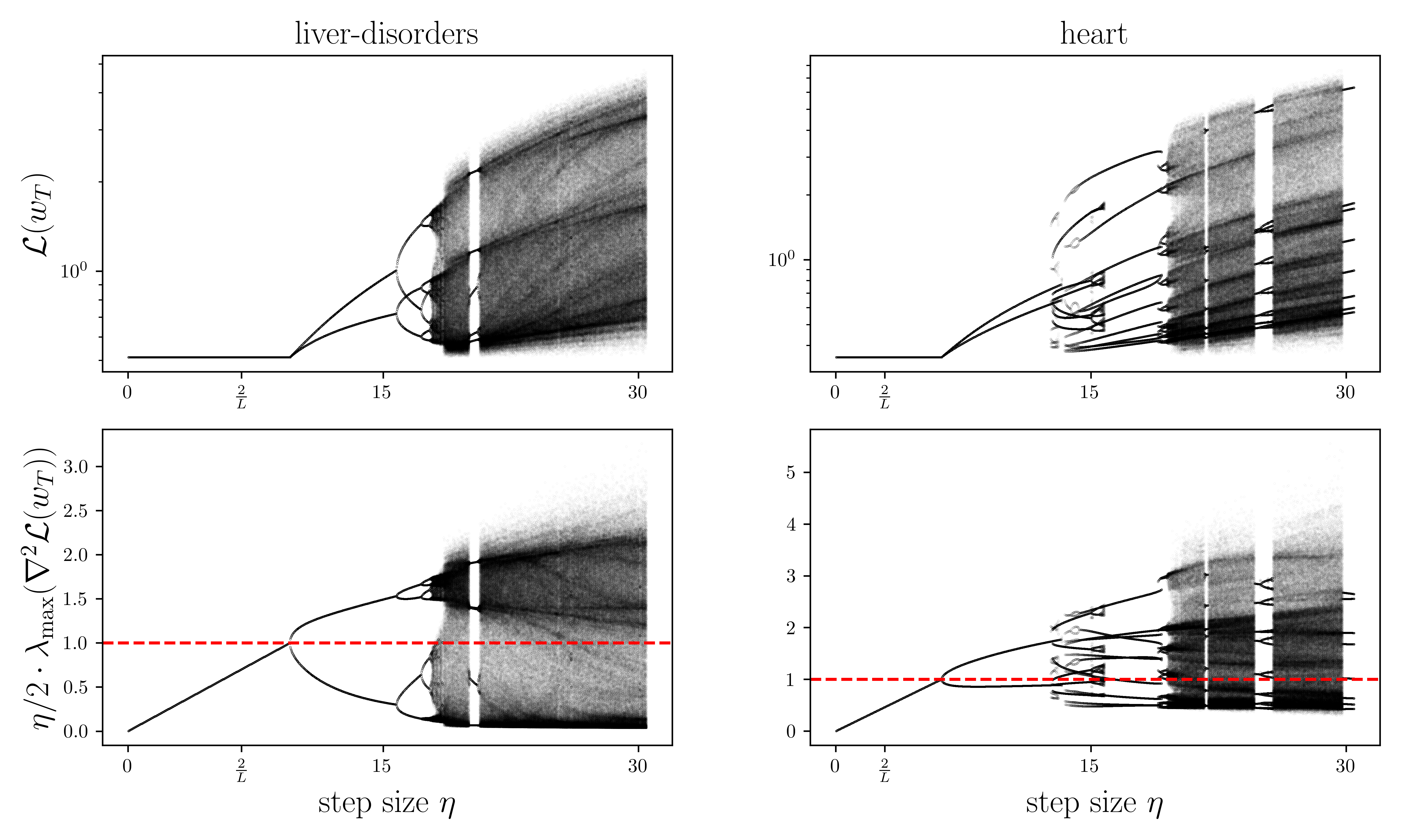
Figure 1: Bifurcation diagrams on two binary classification datasets from Chang and Lin (2011), both are non-separable. For each step size, we run GD for $T=5\cdot 10^{5}$ iterations with $1024$ different random initializations of varying scales. Each point corresponds to the loss (first row) or the (scaled) largest eigenvalue of the Hessian (second row) evaluated at the final iterate $w_{T}$. When multiple points are visible, GD either converged to a cycle or is chaotic under that step size.

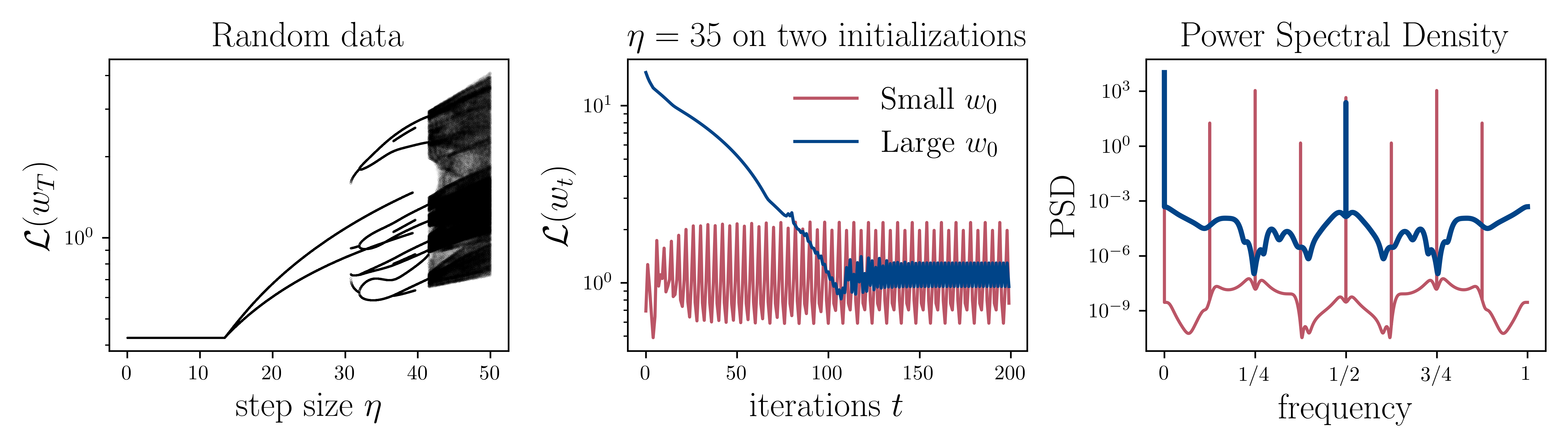
Figure 2: On the left is the bifurcation diagram on a synthetic dataset with $n=12$ and $d=4$. The $x_{i}$’s are generated from the standard Gaussian distribution, with uniformly random labels. In the middle, we plot the loss at each GD iteration when ran with $\eta=35$, for two different initializations $w_{0}=100\cdot\mathbf{1}$ and $w_{0}=0.001\cdot\mathbf{1}$, where $\mathbf{1}$ is the all $1$’s vector. On the right, we compute the power spectral density of the losses over $t$, which shows a period-$2$ cycle for the large initialization, while the small initialization run converged to a period-$8$ cycle.

A remark about Figure 1 is on the “discontinuous” regions in the bifurcation diagram on the heart dataset (right panel), around $\eta=15$. These regions correspond to different cycles arrived at when starting at initializations of various scales, and can be reproduced on a synthetic dataset shown in Figure 2. The discontinuous regions are also present (around $\eta=35$). We then ran GD with $\eta=35$ using two arbitrary initializations that differ in scale, and observe that GD can converge to different cycles of different periods.

The fact that GD undergoes period-doubling bifurcation on the logistic regression objective is perhaps not so surprising — this phenomenon has long been observed and studied on numerous nonlinear maps (Strogatz, 2018). Unlike GD on linear regression which results in a linear map in discrete time, the sigmoid link in the gradient adds a nonlinearity that gives rise to a much richer spectrum of behaviour. What the bifurcation diagrams can help us see is at what step size we cease to have convergence to $w^{*}$. To further our understanding, consider the gradient and Hessian of 1:

$$\nabla{\mathcal{L}}(w)=\frac{1}{n}\sum_{i=1}^{n}\sigma(-w^{\mathsf{\scriptscriptstyle T}}x_{i})(-x_{i}),\quad\nabla^{2}{\mathcal{L}}(w)=\frac{1}{n}\sum_{i=1}^{n}\sigma^{\prime}(-w^{\mathsf{\scriptscriptstyle T}}x_{i})x_{i}x_{i}^{\mathsf{\scriptscriptstyle T}},$$ (3)

where $\sigma(z)=1/(1+\exp(-z))$ is the sigmoid function. We will use $\lambda$ to denote $\lambda_{\max}(\nabla^{2}{\mathcal{L}}(w^{*}))$. As the Hessian is maximized at $w=0$, the global upper bound on the Hessian is given by $L=XX^{\mathsf{\scriptscriptstyle T}}/(4n)$, where $X\in\mathbb{R}^{n\times d}$ is the feature matrix. One interesting observation from Figure 1 lies in the second row, where we plot the final values of $\lambda_{\max}(\nabla^{2}{\mathcal{L}}(w_{T}))$, scaled by $\eta/2$. For all step sizes smaller than $2/L$, this value is clearly convergent, as $w_{t}$ converges to $w^{*}$ regardless of initialization. It appears that GD remains convergent beyond $\eta=2/L$ until $\eta=2/\lambda$, at which period-$2$ cycles begin to appear. This is reasonable as $w^{*}$ is the fixed point of the GD map $T(w)=w-\eta\nabla{\mathcal{L}}(w)$, and first-order stability of $w^{*}$ is guaranteed if the eigenvalues of the Jacobian of $T$

$$J_{T}(w)=I-\eta\nabla^{2}{\mathcal{L}}(w)$$

lie strictly within the unit circle (Sayama, 2015, Chapter 5.7). As a result, $\eta<2/\lambda$ is a necessary condition for GD to converge to $w^{*}$. Next, we illustrate on a toy dataset that the gap between $2/L$ and $2/\lambda$ can grow arbitrarily large, and that analyzing the cycles is very challenging.

3.1 A toy dataset

Consider $n\geq 2$ examples such that $y_{i}=1$ for all $i$. Let $v$ be an arbitrary point on the $d$-dimensional unit sphere. The dataset consists of $n-1$ copies of $v$, and a single copy of $-v$. Clearly, this dataset is not separable by any linear classifier that goes through the origin. The gradient and Hessian simplifies to (see Appendix C)

$$\nabla{\mathcal{L}}(w)=\frac{1}{n}\left(n\cdot\sigma(v^{\mathsf{\scriptscriptstyle T}}w)-(n-1)\right)v\quad\text{and}\quad\nabla^{2}{\mathcal{L}}(w)=\sigma^{\prime}(v^{\mathsf{\scriptscriptstyle T}}w)\cdot vv^{\mathsf{\scriptscriptstyle T}}.$$

Setting the gradient to $0$ gives us $\sigma(v^{\mathsf{\scriptscriptstyle T}}w^{*})=\frac{n-1}{n}$. Since the largest eigenvalue of $vv^{\mathsf{\scriptscriptstyle T}}$ is $1$,

$$\lambda=\sigma(v^{\mathsf{\scriptscriptstyle T}}w^{*})(1-\sigma(v^{\mathsf{\scriptscriptstyle T}}w^{*}))=\frac{n-1}{n^{2}},$$

while globally $L=1/4$. So for large $n$, the gap between $2/L$ and $2/\lambda$ grows quickly.

This toy dataset can also help us get a sense of how difficult it is to analyze these cycles. Note that this problem is degenerate in the sense that $X$ is rank-$1$, so the resulting objective is not strictly-convex and there exists a subspace of minimizers. Instead, we analyze the associated GD update on the probability space. For $i=1,\dots,n$, let $p_{t,i}\coloneqq\sigma(-y_{i}w_{t}^{\mathsf{\scriptscriptstyle T}}x_{i})$. A recurrence relation for $p_{t,i}$ can be derived as follows — simply take the inner product with $-y_{i}x_{i}$ on both sides of the GD update 2 and apply the sigmoid function, giving us

$$p_{t+1,i} \coloneqq\sigma\left(\sigma^{\scriptscriptstyle-1}(p_{t,i})-\frac{\eta}{n}y_{i}\left({\sum_{j=1}^{n}}y_{j}p_{t,j}x_{j}^{\mathsf{\scriptscriptstyle T}}\right)x_{i}\right)\quad i=1,\dots,n,$$ (4)

where $\sigma^{\scriptscriptstyle-1}(p)=\ln\left(\nicefrac{{p}}{{1-p}}\right)$ is the logit function, and $p_{0,i}=\sigma(-y_{i}w_{0}^{\mathsf{\scriptscriptstyle T}}x_{i})$.

On the toy dataset, this update can be simplified into

$$p_{t+1,n} =\sigma\left(\sigma^{\scriptscriptstyle-1}(p_{t,n})-\frac{\eta}{n}\left(p_{t,n}-(n-1)(1-p_{t,n})\right)\right)$$

$$p_{t+1,i} =1-p_{t+1,n}\quad\forall i=1,\dots,n-1.$$ (5)

For $n=2$ and $\eta\geq 2/\lambda=8$, the two points of oscillation are given by the two values of

$$p_{n}=\frac{1}{2}\left(h^{\scriptscriptstyle-1}\left(\frac{\eta}{8}\right)+1\right),$$ (6)

where $h(z)=\tanh^{\scriptscriptstyle-1}(z)/z$ (see Proposition 2 in the Appendix for the derivation). Since $h(z)\geq 1$ for all $z$, the period-$2$ point $p_{n}$ is only defined when $\eta/8\geq 1$, as expected. This shows that even with $n=2$ on this trivially-constructed dataset, computing the two points of oscillation is a nontrivial task as $h^{\scriptscriptstyle-1}$ is not even an elementary function.

4 Technical setup

We now provide the technical setup for analyzing convergence and cycles in the large step size setting. Consider the linear classification problem with loss function $\ell$ of finding

$$w^{*}\in\operatorname*{arg\,min}_{w\in\mathbb{R}^{d}}{\mathcal{L}}(w)=\smash{\frac{1}{n}\sum_{i=1}^{n}\ell(-y_{i}w^{\mathsf{\scriptscriptstyle T}}x_{i})}$$ (7)

where $y_{i}\in\left\{-1,1\right\}$, $x_{i}\in\mathbb{R}^{d}$, and $\ell$ is the loss function on a single example. We are particularly interested in the case where the data is not linearly-separable.

Definition 1 (Non-separability).

For all $w\in\mathbb{R}^{d}$, there exists $i\in\left\{1,\dots,n\right\}$ such that $y_{i}w^{\mathsf{\scriptscriptstyle T}}x_{i}<0$.

While our motivation is to study the behaviour of GD on logistic regression under large step sizes, our results will be stated in terms of general loss functions $\ell$ satisfying the following set of assumptions.

Assumption 1.

The loss function on the individual examples $\ell:\mathbb{R}\to\mathbb{R}_{+}$ satisfies:

1. $\ell$ is three-times continuously-differentiable and strictly convex, and $\lim_{z\to-\infty}\ell(z)=0$.

2. $\lim_{z\to-\infty}\ell^{\prime}(z)=0$ and $\lim_{z\to\infty}\ell^{\prime}(z)=1$,

3. $\ell^{\prime\prime}$ is increasing on $(-\infty,0]$ and decreasing on $[0,\infty)$; furthermore, it decays fast enough that

   $$\lim_{\epsilon\to 0}\;\frac{1}{\epsilon^{2}}\ell^{\prime\prime}\left(\frac{1}{\epsilon}\right)=0.$$

The limit of $\ell$ and the upper bound on $\ell^{\prime}$ can both be generalized to any finite positive value.

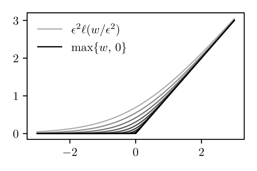
Figure 3: The limit in 8 using the logistic loss as an example. Darker grey represents smaller values of $\epsilon$.

This set of assumptions essentially requires that $\ell$ looks like a ReLU when zoomed out.

Corollary 1.

Assumption 1 implies that

$$\lim_{\epsilon\to 0}\epsilon^{2}\ell\left(\frac{z}{\epsilon^{2}}\right)=\max\left\{z,\,0\right\}.$$ (8)

The logistic loss $\ell(z)=\log(1+\exp(z))$ and the squareplus function $\ell(z)=0.5(\sqrt{4+z^{2}}+z)$ (Barron, 2021) both satisfy Assumption 1, as verified in Section D.1. Outside of these two losses, there are few commonly-used machine learning loss functions that satisfy our assumptions. The purpose of stating our results in this way is to emphasize that our results are not an algebraic consequence of the logistic loss, but rather, a consequence of its structural properties.

5 One-dimensional case

As discussed in the previous section, although $\eta<2/\lambda$ is a necessary condition for convergence, it is not sufficient. Specifically, it only guarantees local convergence to $w^{*}$ when we initialize within a neighborhood of $w^{*}$. From Figure 1, it appears that we do converge globally for all $\eta<2/\lambda$, as the initializations we used vary in scale. However, as we show later, this is not the case for all datasets. The first natural question to ask is what is a sufficient condition on the step size to guarantee global convergence? As it turns out, when $d=1$, this step size is given by $\eta<1/\lambda$.

Theorem 1.

Suppose Assumption 1 holds for the classification problem in $1$ dimension with non-separable data, that is, $w^{*}$ is finite. Then the GD iterates $\left\{w_{t}\right\}$ converge to $w^{*}$ when $\eta\leq 1/{\mathcal{L}}^{\prime\prime}(w^{*})$ for any initialization $w_{0}$. Moreover, if we choose $\eta=1/{\mathcal{L}}^{\prime\prime}(w^{*})$, then for all $\epsilon>0$, it holds that $(w_{\tau}-w^{*})^{2}\leq\epsilon$ for some

$$\tau\leq 1+\max\left\{0,-w_{0}\cdot\operatorname{sign}(w^{*})\cdot{\mathcal{L}}^{\prime\prime}(w^{*})/{\mathcal{L}}^{\prime\prime}(0)\right\}+{\mathcal{O}}(\log(1/\epsilon)).$$

Convergence is straightforward. Suppose $w^{*}>0$. The interval ${\mathcal{I}}=[w^{*},+\infty)$ is an invariant set under the step size requirement, that is, if $w_{t}\in{\mathcal{I}}$, then $w_{t+1}\in{\mathcal{I}}$. Furthermore, $w_{t}$ converges to $w^{*}$ on ${\mathcal{I}}$. So either we converge directly in ${\mathcal{I}}$, or we initialize in $(-\infty,w^{*})$, from which we either approach $w^{*}$ form the left, or cross over into ${\mathcal{I}}$ , within which convergence is guaranteed. The detailed proof including the rate can be found in Section A.1. The next result shows that if we increase the step size beyond $1/{\mathcal{L}}^{\prime\prime}(w^{*})$, global convergence is no longer guaranteed.

Theorem 2.

Suppose Assumption 1 holds and $d=1$. Then for all $\gamma\in(1,2]$, there exists a non-separable classification problem on which a GD trajectory under the step size $\eta=\gamma/{\mathcal{L}}^{\prime\prime}(w^{*})$ converges to a cycle of period $k>1$.

It is worth emphasizing that Theorem 2 does not imply that a cycle is possible for every dataset. It only shows that if we were to first pick a $\gamma\in(1,2]$, then we can construct a dataset such that GD with step size $\eta=\gamma/{\mathcal{L}}^{\prime\prime}(w^{*})$ can converge to a cycle. Note that this construction implies $\eta>2/L$ where $L={\mathcal{L}}^{\prime\prime}(0)$ is the global smoothness constant, as otherwise we would have global convergence. Stability of the cycle coexists with stability of the solution $w^{*}$. Therefore, depending on the initialization, GD may still converge to $w^{*}$ with the same step size. Moreover, given an arbitrary dataset, it is not always easy to verify whether a cycle exists before hitting the $2/\lambda$ step size. In fact, when we ran GD using many different initializations of varying scales in on real datasets (Figure 1), we did not see a clear cycle emerging at all until $\eta=2/\lambda$. We now present the main proof steps.

Proof sketch.

Fix a $\gamma\in(1,2]$, we begin by constructing a dataset where the $x_{i}$’s are copies of $1$’s and $-1$’s, with all $1$’s label. This dataset corresponds to a loss ${\mathcal{L}}$ such that the minimizer is $w^{*}>0$ without loss of generality. On this ${\mathcal{L}}$, it can be shown that a trajectory of the form

$$w_{k}<0<w_{k-1}<\dots<w_{0}$$ (9)

exists. Each iterate is generated via the GD update on ${\mathcal{L}}$ with step size $\eta=\gamma/{\mathcal{L}}^{\prime\prime}(w^{*})$, illustrated in the left panel of Figure 4. Furthermore, we can ensure that $0<w_{k+1}<w_{0}$.

Then, consider perturbing ${\mathcal{L}}$ by adding a ReLU to it, giving us

$${\mathcal{L}}_{\text{perturbed}}(w)={\mathcal{L}}(w)+\frac{w_{0}-w_{k+1}}{\eta}\max\left\{-w,\,0\right\}.$$ (10)

Observe that the ReLU does not contribute any additional curvature on top of ${\mathcal{L}}$, and it also does not contribute any gradient to all points $w>0$. Therefore, the minimizer remains the same. So if we were to run GD starting at the same $w_{0}$ on ${\mathcal{L}}_{\text{perturbed}}$ with the step size $\eta_{\text{perturbed}}=\gamma/{\mathcal{L}}^{\prime\prime}_{\text{perturbed}}(w^{*})=\eta$, the new trajectory would coincide with the original trajectory up to step $k$. Let $\tilde{w}_{t}$ denote the iterates of this new trajectory for $t\geq 0$. At point $\tilde{w}_{k}=w_{k}<0$, the ReLU becomes active. Applying one GD update at this point leads to

$$\tilde{w}_{k+1} =\tilde{w}_{k}-\eta{\mathcal{L}}^{\prime}_{\text{perturbed}}(\tilde{w}_{k})$$ (11)

$$=\tilde{w}_{k}-\eta{\mathcal{L}}^{\prime}(\tilde{w}_{k})+\eta\frac{w_{0}-w_{k+1}}{\eta}$$

$$=w_{k+1}+w_{0}-w_{k+1}$$

$$=w_{0},$$

resulting in a cycle. As shown in the second panel of Figure 4, we have effectively added enough gradient to the left of the minimizer such that $\tilde{w}_{k+1}$ gets kicked right back to where we started.

However, adding a ReLU to a loss function of the form 7 does not automatically yield a valid classification problem. We need to show that this can be achieved equivalently by adding more examples to the dataset. Recall that by Corollary 1, this ReLU is the limit of the function $\ell_{\epsilon}(w)=\epsilon^{2}\ell\left(-w/\epsilon^{2}\right)$ as $\epsilon\to 0$ (Figure 3 and Corollary 1). This allows us to define a continuous perturbation

$${\mathcal{L}}_{\epsilon}(w)={\mathcal{L}}(w)+\frac{w_{0}-w_{k+1}}{\eta}\ell_{\epsilon}(w).$$ (12)

It remains to invoke the implicit function theorem to argue that there exists a non-zero $\epsilon$ such that $\epsilon^{2}(w_{0}-w_{k+1})/\eta>0$ is rational. This implies we can obtain a loss function equivalent to adding integer copies of the example $x=1/\epsilon^{2}$ of label $y=1$ to the original dataset. This ensures that ${\mathcal{L}}_{\epsilon}$ indeed corresponds to an objective on a valid binary classification dataset.

Finally, we argue that this cycle is locally stable. This can be achieved by observing that at all points on this cycle (except for the one to the left of $w^{*}$) have a Hessian strictly smaller than that at $w^{*}$ (Assumption 1). This is sufficient to guarantee that the Jacobian of the $k+1$-th iterate GD map has a magnitude strictly less than one (if this is not the case, we can extend the trajectory backwards from $w_{0}$ to $w_{-1}$, $w_{-2}$, …, until satisfied). Local stability implies that if we initialize sufficiently close to the cycle (rather than the minimizer), GD would converge to this cycle instead.

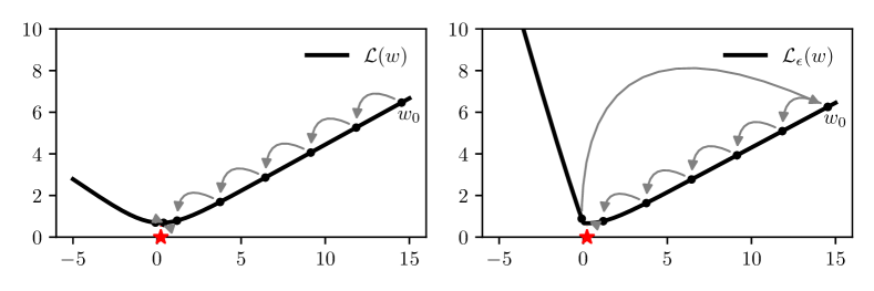
Figure 4: Illustration of our cycle construction. On the left, ${\mathcal{L}}$ is the logistic loss with data consisting of $250$ copies of $x_{i}=1$ and $200$ copies of $x_{i}=-1$. On top of this dataset we add $15$ copies of $x_{i}=70$ to get ${\mathcal{L}}_{\epsilon}$ on the right. The red star marks the minimizer $w^{*}$ and $w^{*}_{\epsilon}$ of the respective objective. Starting at the same $w_{0}$ and using the same $\gamma=1.5$, GD on ${\mathcal{L}}$ with $\eta=\gamma/{\mathcal{L}}^{\prime\prime}(w^{*})$ converges to the minimizer, while GD on ${\mathcal{L}}_{\epsilon}$ with $\eta_{\epsilon}=\gamma/{\mathcal{L}}_{\epsilon}^{\prime\prime}(w^{*}_{\epsilon})$ converges to a period-$7$ cycle.

∎

As verifying the assumptions of the implicit function theorem can be technical and tedious, we defer the full proof to Section A.2. In Figure 5, we illustrate that one can easily construct a dataset for different values of $\gamma\in(1,2]$ such that GD converges to cycles. A pattern to note is that the smaller the $\gamma$, the longer period the cycle tends to have, as it takes more steps to move along the “flatter” side of the loss before being kicked back. Note that convergence to $w^{*}$ and stable cycles are not necessarily the only two events that can happen below the $2/\lambda$ step size. If for some dataset there exists a period-$3$ cycle under the step size $\eta=\gamma/\lambda$ for some $\gamma<2$, then a chaotic GD trajectory can also occur for that dataset under the same $\gamma$ (Li and Yorke, 1975).

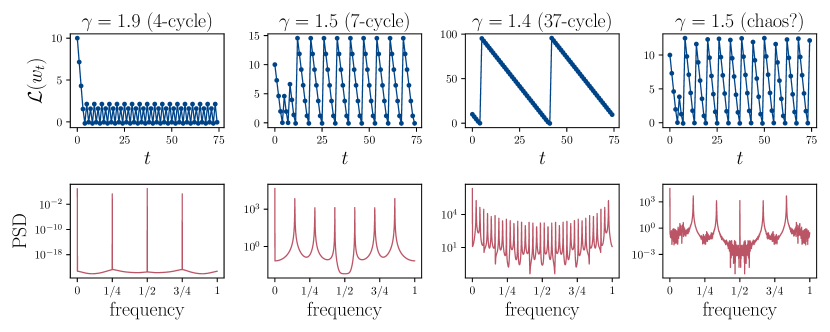
Figure 5: For each $\gamma$, we construct a one-dimensional dataset such that GD on this problem with the logistic loss converges to a stable cycle under the step size $\eta=\gamma/{\mathcal{L}}^{\prime\prime}(w^{*})$. One exception is the last column which seems to suggest GD can even be chaotic when $\gamma<2$. Figures in the first row show the loss evaluated at successive iterates, while the second row shows the power spectral density of the losses at the last $1024$ iterations. Details on each dataset are in Appendix E.

6 Higher dimensions

In the one-dimensional case, we have shown that under the step size $\eta=\gamma/{\mathcal{L}}^{\prime\prime}(w^{*})$, convergence is guaranteed for all $\gamma\leq 1$, while increasing $\gamma$ beyond $1$ can lead to cycles. In higher dimensions, we no longer have global convergence even in the small $\gamma$ case. As we now show, for all $\gamma\in(0,1]$, a cycle can be constructed in $d=2$ using similar techniques. Since we can embed the constructed dataset in higher dimensions, the result trivially extends to any non-linearly-separable classification problem satisfying Assumption 1 of dimension $d>1$.

Theorem 3.

Suppose Assumption 1 holds and $d=2$. Then for all $\gamma\in(0,1]$, there exists a non-separable classification problem on which a GD trajectory under the step size $\eta=\gamma/\lambda$ converges to a cycle of period $k>1$, where $\lambda=\lambda_{\max}(\nabla^{2}{\mathcal{L}}(w^{*}))$.

The idea of the proof is similar to that of Theorem 2. We briefly discuss the technique and main differences here and defer the full proof to Section B.1.

Proof sketch.

Fix a $\gamma\in(0,1]$, we construct a base dataset corresponding to a loss ${\mathcal{L}}$ such that the minimizer is strictly positive. We show that there exists a trajectory that moves almost in a straight line towards the minimizer, as in the first plot of Figure 6. Let this trajectory be $w_{0},w_{1},\dots$, up to $w_{k}$, and $T(w)=w-\eta\nabla{\mathcal{L}}(w)$ be the GD update on ${\mathcal{L}}$.

We then perturb ${\mathcal{L}}$ by adding two ReLUs to it. Define

$${\mathcal{L}}_{\text{perturbed}}(w)={\mathcal{L}}(w)+c_{1}\max\left\{-w^{\mathsf{\scriptscriptstyle T}}p,\,0\right\}+c_{2}\max\left\{-w^{\mathsf{\scriptscriptstyle T}}q,\,0\right\},$$ (13)

for some constants $c_{1},c_{2}>0$ and vectors $p$ and $q$. Specifically, $p$ and $q$ are positioned such that the minimizer of ${\mathcal{L}}_{\text{perturbed}}$ is identical to that of ${\mathcal{L}}$. Let $\left\{\tilde{w}_{t}\right\}$ be the trajectory of running GD on ${\mathcal{L}}_{\text{perturbed}}$ with the step size $\eta=\gamma/\lambda_{\max}(\nabla^{2}{\mathcal{L}}_{\text{perturbed}}(w^{*}))=\eta$, and the same initialization $\tilde{w}_{0}=w_{0}$.

Observe that the two ReLUs are activated for all points above the line $w^{\mathsf{\scriptscriptstyle T}}p=0$ and below the line $w^{\mathsf{\scriptscriptstyle T}}q=0$. We design our original trajectory such that neither gets activated until $w_{k-1}$, thus the two trajectories coincide for all $w_{t}$ from $t=0$ to $t=k-2.$ At $\tilde{w}_{k-1}=w_{k-1}$, we cross over $w^{\mathsf{\scriptscriptstyle T}}p=0$, the first ReLU is activated, kicking the perturbed trajectory in the orthogonal direction to $\tilde{w}_{k}$ (as in the middle plot of Figure 6). At this new point $\tilde{w}_{k}$, we carefully set $c_{1}$, $c_{2}$, $p$ and $q$ such that the first ReLU becomes inactive while the second activates, and that another GD step takes us back to $w_{0}$.

As in the one-dimensional case (Theorem 2), we then use the fact that ${\mathcal{L}}_{\text{perturbed}}$ is the limit of a continuous perturbation for which we can find a valid classification dataset. Stability of the resulting cycle is also straightforward.

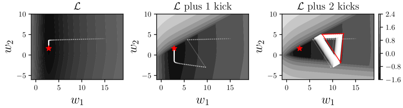
Figure 6: Illustration of our cycle construction in two dimensions using the logistic loss. The objective (in log scale) in the middle and right contours are created by adding large-magnitude examples to the dataset underlying ${\mathcal{L}}$, depicted on the left. Red stars mark the minimizer $w^{*}$ of the respective losses. Starting at the same $w_{0}$ using the same $\gamma=0.4$, GD on ${\mathcal{L}}$ and ${\mathcal{L}}$ with one set of additional data points both converge to the solution. When we add in the second set of data points, GD converges to a period-$13$ cycle. The trajectory in white marks the first $500$ steps, while the final $20$ steps are marked in red. Details on the synthetic dataset are in Appendix E.

∎

It is worth noting that by this construction, it appears that we cannot obtain a cycle of period exactly $2$ as the perturbation involves $2$ kicks, and so the length of the cycle is at least $3$. Nonetheless, one can easily construct a period-$2$ cycle by simply raising $\gamma$ to be between $1$ and $2$, so that the trajectory can cross over $0$ in the first coordinate, to the left of which we can add just one ReLU to kick us back to $w_{0}$ in just one step. As our goal is to show that in the two dimensional case, GD can converge to cycles on certain datasets when $\gamma\leq 2$, what we have proven is already sufficient. Although our result is only for the two-dimensional setting, it can easily be generalized to any dimension $d>1$.

Corollary 2.

Suppose Assumption 1 holds and $d>1$. Then for all $\gamma\in(0,1]$, there exists a non-separable classification problem on which a GD trajectory under the step size $\eta=\gamma/\lambda$ converges to a cycle of period $k>1$, where $\lambda=\lambda_{\max}(\nabla^{2}{\mathcal{L}}(w^{*}))$.

Proof.

By Theorem 3, there exists a dataset in two dimensions such that the statement holds. Let $Z\in\mathbb{R}^{n\times 2}$ and label vector $y$ be this dataset, and $u^{*}\in\mathbb{R}^{2}$ be the minimizer of the corresponding loss. We lift this dataset to higher dimensions by simply padding $0$’s to each example $x_{i}$ in $X$ until it is a vector of dimension $d$. Let $x_{i}=(z_{i,1},z_{i,2},0,\dots,0)\in\mathbb{R}^{d}$ where $d>2$ for each $i=1,\dots,n$, and $w^{*}=(u^{*}_{1},u^{*}_{2},0,\dots,0)\in\mathbb{R}^{d}$. Observe that $w^{*}$ is a minimizer of the loss on the new dataset $(X,y)$, because the loss is convex and

$$\nabla{\mathcal{L}}(w^{*})=\frac{1}{n}\sum_{i=1}^{n}\ell^{\prime}(-y_{i}x_{i}^{\mathsf{\scriptscriptstyle T}}w^{*})(-y_{i}x_{i})=\frac{1}{n}\sum_{i=1}^{n}\ell^{\prime}(-y_{i}z_{i}^{\mathsf{\scriptscriptstyle T}}u^{*})(-y_{i}x_{i})$$

which is just $\nabla{\mathcal{L}}(u^{*})=0$ but padded with more zeros. Similarly, we also have $\lambda_{\max}(\nabla^{2}{\mathcal{L}}(u^{*}))=\lambda_{\max}(\nabla^{2}{\mathcal{L}}(w^{*}))$, thus the step sizes used on the two datasets are the same under the same $\gamma$. Therefore, we can take the cycle in the two-dimensional dataset, pad each point on the orbit by $0$’s to obtain a cycle in the higher dimension. ∎

7 Discussion

We consider GD dynamics on classification tasks where the objective shares similar properties as that of logistic regression. Specifically, we study convergence behaviour when the problem is not linearly separable, and show that as the step size increases, GD follows a period-doubling route to chaos. We prove that although $\eta<2/\lambda$ is a necessary condition for global convergence, it is not sufficient, in that GD can converge to stable cycles below this step size on certain datasets. One limitation of our work is that beyond the one-dimensional setting, we still do not have a sufficient condition above the $2/L$ step size for which global convergence is guaranteed. Additionally, our analysis does not provide any practical recommendation — even in one-dimension when the sufficient $1/\lambda$ step size is potentially greater than $2/L$, it is still impossible to know what $\lambda$ is without first finding the solution. Nevertheless, we hope our study provides insights into analyzing GD convergence with large step sizes on more general tasks involving the logistic or the crossentropy loss.

Although the results are mostly negative on the global convergence of GD above the $2/L$ step size, the way we construct our cycles already contains an interesting observation: it seems that the datasets we construct to generate a cycle all require a few massive “outliers”. These outliers are responsible for the large gradients on one side of the objective that kick our trajectory back to the starting location. Indeed, the real datasets that we used to generate Figure 1 both have features scaled within the $[-1,1]$ range. This scaling is perhaps why it appears that all runs below the critical $2/\eta$ step size actually converged to the minimizer, despite using a large scale for initializations. The reason we chose scaled data is to improve the conditioning so that GD can converge within a reasonable number of steps under tiny step sizes, so that generating the bifurcation diagrams can be done in a reasonable amount of time. This naturally raises some interesting questions. Does data normalization or feature scaling (i.e. requiring $\|x_{i}\|=1$) allow GD to converge with even larger step sizes, potentially up to $2/\lambda$? Does it explain why techniques such as layer normalization (Ba et al., 2016) in deep neural networks help stabilize training? We leave these questions to future work.

Acknowledgments and Disclosure of Funding We would like to thank Frederik Kunstner, Aaron Mishkin, Liwei Jiang, and Sharan Vaswani for helpful discussions and feedback on the manuscript. S.M. was partially supported by the NSERC PGS-D award (PGSD3-547276-2020). A.O. acknowledges the financial support of the Hector Foundation. C.D. was supported by the NSF CAREER Award (2046760).

Appendix A Proofs in one dimension

For all proofs in this section, we assume without loss of generality that $y_{i}=1$ for all $i$. If $y_{i}=-1$ for some $i$, we can simply flip the corresponding $x_{i}$ to $-x_{i}$ to obtain the same objective. We use $T$ to denote the GD map with a constant step size $\eta$

$$T(w)\coloneqq w-\eta{\mathcal{L}}^{\prime}(w).$$ (14)

Recall our Assumption 1 which holds for the logistic loss. See 1

A.1 Convergence under the stable step size

See 1

Proof.

We assume without loss of generality that $w^{*}>0$. If $w^{*}=0$, then fact that ${\mathcal{L}}^{\prime\prime}$ is maximized at $0$ implies $T$ is Lipschitz with a constant strictly less than $1$ (because ${\mathcal{L}}^{\prime\prime}(w^{*})>0$ when the data is non-separable). Therefore $T$ is a contraction which implies global convergence. If $w^{*}<0$, we can flip the signs of all the $x_{i}$’s and get $w^{*}>0$ as the problem is symmetric about $0$. The proof is split into three cases based on the initialization:

Case 1: $w_{0}>w^{*}$. By Assumption 1, $\ell^{\prime\prime}$ is decreasing on $[0,\infty)$, and so $\ell^{\prime}$ is concave on this interval, therefore

$${\mathcal{L}}^{\prime}(w) \leq{\mathcal{L}}^{\prime}(w^{*})+{\mathcal{L}}^{\prime\prime}(w^{*})(w-w^{*})$$

$$={\mathcal{L}}^{\prime\prime}(w^{*})(w-w^{*}).$$ (15)

And so if $w>w^{*}$,

$$T(w)\geq w-\eta\left({\mathcal{L}}^{\prime\prime}(w^{*})(w-w^{*})\right)\geq w^{*}$$

using the upper bound on the step size. Since we will always move towards the left when $w>w^{*}$, convergence is thus guaranteed as ${\mathcal{I}}=[w^{*},+\infty)$ is an invariant set. Furthermore, ${\mathcal{L}}^{\prime\prime}$ is maximized at $w^{*}$ over ${\mathcal{I}}$, and is ${\mathcal{L}}^{\prime\prime}(w_{0})$-strongly convex over the bounded subset $[w^{*},w_{0}]$. Then for any $t>0$ starting at $w_{0}$, the classic strongly-convex analysis (for instance Garrigos and Gower (2023)) gives

$$(w_{t}-w^{*})^{2} \leq\left(1-\eta{\mathcal{L}}^{\prime\prime}(w_{0})\right)^{t}(w_{0}-w^{*})^{2}$$ (16)

for all $\eta\leq 1/{\mathcal{L}}^{\prime\prime}(w^{*})$.

For all $w_{0}<w^{*}$, each GD step takes us to the right, and so we either approach $w^{*}$ from the left, or cross over into ${\mathcal{I}}$ within which convergence is already established. When we do cross over at some $w<w^{*}$, the farthest we can land on the right is given by

$$T(w) \leq w^{*}-\eta{\mathcal{L}}^{\prime}(w)$$

$$\leq w^{*}-\eta\lim_{w\to-\infty}{\mathcal{L}}^{\prime}(w)$$

$$=\underbrace{w^{*}-\eta C}_{\bar{w}}$$ (17)

for some constant $C$ due to boundedness of $\ell^{\prime}$. As $\bar{w}$ does not depend on $t$, we can never move arbitrarily far to the right. It remains to establish the iteration complexity.

Case 2: $w_{0}<0$. In this case, the maximum number of iterations for us to arrive at $w_{\tau}\geq 0$ is given by

$$\tau=\lceil\frac{-w_{0}}{\eta\cdot{\mathcal{L}}^{\prime}(0)}\rceil$$ (18)

which holds for all $\eta>0$. This is because while ${\mathcal{L}}^{\prime}<0$, it is decreasing in magnitude as we increase from $w_{0}$ to $0$.

Case 3: $0\leq w_{0}\leq w^{*}$. In this interval, we can use A.1 again and use $\eta=1/{\mathcal{L}}^{\prime\prime}(w^{*})$ to get

$$T(w_{0}) \geq w_{0}-\eta({\mathcal{L}}^{\prime\prime}(w^{*})(w_{0}-w^{*}))=w^{*}.$$

So in this interval, we cross over into ${\mathcal{I}}$ in one step. Combining 16, 18 and A.1, we have that after at most $1+\max\left\{0,\,-w_{0}\cdot{\mathcal{L}}^{\prime\prime}(w^{*})/{\mathcal{L}}^{\prime\prime}(0)\right\}$ number of iterations, we will enter ${\mathcal{I}}$, from which convergence is guaranteed at a linear rate. The rate depends on $\eta=1/{\mathcal{L}}^{\prime\prime}(w^{*})$ as well as $\bar{w}$ if we did not initialize in ${\mathcal{I}}$. If $w^{*}<0$, then the initial number of iterations kick in when $w_{0}>0$ and the entire argument holds with a sign flip. This completes the proof. ∎

A.2 Cycle construction below the critical step size

See 2

Proof.

We will construct for all $\gamma\in[1,2)$ a dataset for which the objective is given by

$${\mathcal{L}}(w)=\sum_{i=1}^{n+m}\ell\left(-y_{i}x_{i}w\right),$$

in which all labels $y_{i}=1$, and there are $n$ copies of $x_{i}=-1$, and $m>n$ copies of $x_{i}=1$, such that $w^{*}>0$. We drop the scaling factor $1/(n+m)$ for simplicity. By Lemmas 1 and 2, there exists a valid combination of $n$ and $m$ such that a GD trajectory of the form

$$w_{k}<0<w_{k-1}<\dots<w_{1}<w_{0}$$ (19)

is possible for some $k>2$, under the step size $\eta$ where $w_{t+1}=T(w_{t})$ for $t=0,1,\dots,k-1$. We also assume that $w_{0}>T(w_{k})$. This is valid since if it’s not the case, we can use Lemma 2 to extend the trajectory further to the right as $w_{0}<w_{-1}<\dots<w_{-t}$ until $w_{-t}>T(w_{k})$ is satisfied, then relabel the iterations.

Now let’s define the perturbation

$$\ell_{\epsilon}(w)\coloneqq\begin{cases}\epsilon^{2}\cdot\ell\left(-\frac{w}{\epsilon^{2}}\right)&\text{if $\epsilon\neq 0$}\\ \max\{-w,\,0\}&\text{if $\epsilon=0$}\end{cases}$$ (20)

where $a$ is the upper bound on $\ell^{\prime}$ given in Assumption 1. Define constant

$$c\coloneqq\frac{w_{0}-T(w_{k})}{\eta}>0,$$ (21)

where $\eta$ is the step size that generated the trajectory in 19. Then for all $\epsilon$ such that $c\cdot\epsilon^{2}=p/q>0$, the perturbed objective

$${\mathcal{L}}_{\epsilon}(w)\coloneqq{\mathcal{L}}(w)+c\cdot\ell_{\epsilon}(w)$$ (22)

is equivalent to a classification problem on a dataset consisting of $q$ copies of the original examples plus $p$ copies of the example $x=1/\epsilon^{2}$. By Assumption 1,

$$\lim_{\epsilon\to 0}\epsilon^{2}\cdot\ell\left(-\frac{w}{\epsilon^{2}}\right)=a\cdot\max\left\{-w,\,0\right\}$$

and so $\ell_{\epsilon}$ is continuous.

Let $w^{*}_{\epsilon}>0$ be the minimizer of ${\mathcal{L}}_{\epsilon}$ for $\epsilon>0$. We can run GD with the step size $\eta_{\epsilon}=\gamma/{\mathcal{L}}_{\epsilon}^{\prime\prime}(w^{*}_{\epsilon})$ on this perturbed objective 22 using the same $\gamma$ that generated 19. Let

$$T_{\epsilon}(\tilde{w})\coloneqq\tilde{w}-\eta_{\epsilon}{\mathcal{L}}_{\epsilon}^{\prime}(\tilde{w})$$ (23)

be the corresponding GD map. Starting at $\tilde{w}_{0}=w_{0}$ in 19, let $\tilde{w}_{t+1}=T_{\epsilon}(\tilde{w}_{t})$ for $t=0,1\dots,k$. Since $w^{*}_{\epsilon}$, ${\mathcal{L}}^{\prime}_{\epsilon}$, and ${\mathcal{L}}^{\prime\prime}_{\epsilon}$ are all continuous in $\epsilon$ (Lemmas 3 and 4), so is $\eta_{\epsilon}$ and $T_{\epsilon}$, with limits

$$\eta_{\epsilon}\to\eta\quad\text{and}\quad T_{\epsilon}\to T_{0}$$

as $\epsilon\to 0$. Furthermore, for all $w>0$, $\lim_{\epsilon\to 0}\ell^{\prime}_{\epsilon}(w)=0$. Combined with the fact that original trajectory 19 is positive up to $w_{k-1}$, we also have $\tilde{w}_{t}\to w_{t}$ as $\epsilon\to 0$ for all $t=0,1,\dots,k$. We will show that the next step takes us back to $w_{0}$, resulting in a cycle.

Let $G:\mathbb{R}^{2}\to\mathbb{R}$ be defined as

$$G(\epsilon,w)\coloneqq T^{k+1}_{\epsilon}(w)-w=\underbrace{T_{\epsilon}\circ\ldots\circ T_{\epsilon}}_{k+1\text{ times}}(w)-w.$$ (24)

By Lemma 5, $T_{\epsilon}$ is continuously differentiable in $w$ and $\epsilon$ except at $w=0$ and $\epsilon=0$, and so is $T^{k}_{\epsilon}$ as it is a function composition via the chain rule. Consider the point $(\epsilon,w)=(0,w_{0})$. Note that we must have $w_{0}>w^{*}>0$ due to the trajectory construction 19. Evaluating $G$ at this point gives us

$$G(0,w_{0}) =T_{0}(T^{k}_{0}(w_{0}))-w_{0}$$

$$=T_{0}\left(w_{k}\right)-w_{0}$$

$$=w_{k}-\eta L^{\prime}(w_{k})+\eta\cdot c-w_{0} w_{k}<0$$ ()

$$=T(w_{k})+w_{0}-T(w_{k})-w_{0} c$$ (Definition of in 21)

$$=0,$$

resulting in a cycle. In addition, at any $w\neq 0$,

$$T^{\prime}_{\epsilon}(w) =1-\eta_{\epsilon}{\mathcal{L}}^{\prime\prime}_{\epsilon}(w),$$

$$\frac{\partial G}{\partial w}(0,w_{0}) =\prod_{t=0}^{k}\left(1-\eta_{0}{\mathcal{L}}_{0}^{\prime\prime}(T_{0}(\tilde{w}_{t}))\right)-1.$$

Note that for all $t=0,1,\dots,k-1$, $\tilde{w}_{t}=w_{t}>w^{*}$ when $\epsilon=0$ and that $w^{*}=w^{*}_{0}$,

$${\mathcal{L}}^{\prime\prime}_{0}(\tilde{w}_{t})<{\mathcal{L}}_{0}^{\prime\prime}(w^{*}_{0})=\frac{\gamma}{\eta_{0}}$$

and so

$$\left|\prod_{t=0}^{k-1}\left(1-\eta_{0}{\mathcal{L}}_{0}^{\prime\prime}(T_{0}(\tilde{w}_{t}))\right)\right|<\left|(1-\gamma)^{k}\right|\leq 1$$

since $\gamma\in(1,2]$. Observe that we can extend the trajectory 19 to the right as far as needed to guarantee that the product with the last term $(1-\eta_{0}{\mathcal{L}}^{\prime\prime}_{0}(T_{0}(\tilde{w}_{k})))$ term is still less than $1$ in magnitude. This implies

$$\frac{\partial G}{\partial w}(0,w_{0})\neq 0.$$

We have justified the assumptions of the implicit function theorem (Theorem 4) to conclude that there exists a function $\omega:I\to J$ where $I$ is an open interval about $\epsilon=0$ and $J$ is an open interval about $w=w_{0}$ such that $G(\epsilon,\omega(\epsilon))=0$ for all $\epsilon\in I$.

Lastly, we need to show that cycle is stable. Consider the function $\mu:\mathbb{R}^{2}\to\mathbb{R}_{+}$ defined as

$$\mu(\epsilon,w) \coloneqq\left|(T_{\epsilon}^{k+1})^{\prime}(w)\right|=\left|\prod_{t=0}^{k}(1-\eta_{\epsilon}{\mathcal{L}}_{\epsilon}^{\prime\prime}(T^{t}_{\epsilon}(w)))\right|,$$ (25)

which is continuous in $w$ due to continuity of $\ell^{\prime\prime}_{\epsilon}$ in $w$ for all $\epsilon$, as well as continuity of $T_{\epsilon}$ except at $w=0$ and $\epsilon=0$ Lemma 5. By Lemma 3, $\ell_{\epsilon}^{\prime\prime}(w)$ is continuous almost everywhere, and so is ${\mathcal{L}}^{\prime\prime}_{\epsilon}$. Combining Lemma 4 for continuity of $\eta_{\epsilon}$ and Lemma 5 for $T_{\epsilon}$, we have that $\mu$ is continuous in both variables except at $w=0$ and $\epsilon=0$.

We know that $\mu(0,w_{0})<1$ from earlier, and by continuity there must exist a neighbourhood $U$ around $\epsilon=0$ such that $\mu(\epsilon,\omega(\epsilon))<1$ for all $\epsilon\in U$, as $\omega$ is continuous in $\epsilon$. Since $U$ and $I$ are both open, there must exist a nonzero $\epsilon_{0}\in I\cap U$ such that

$$G(\epsilon_{0},\omega(\epsilon_{0}))=0\quad\text{and}\quad\mu(\epsilon_{0},\omega(\epsilon_{0}))<1,$$

implying that the trajectory on the perturbed objective with $\epsilon=\epsilon_{0}$ is a stable cycle. Stability ensures that if initialize close enough to $\omega(\epsilon_{0})$ we will converge to this cycle, as it is a stable fixed point of the $T^{k+1}$ map. A final note is that we can always pick $\epsilon_{0}$ such that $c\cdot\epsilon_{0}^{2}$ is rational, so that the perturbed objective 22 indeed corresponds to a valid classification problem. This completes the proof. ∎

Lemma 1 (Crossing over $w^{*}$).

Suppose the $1$-dimensional classification objective has the form

$${\mathcal{L}}(w)=\frac{1}{n+m}\sum_{i=1}^{n+m}\ell(-y_{i}x_{i}w),$$ (26)

where $y_{i}=1$ for all $i$, and there are $n$ copies of $x_{i}=-1$ and $m>n$ copies of $x_{i}=1$. Let $w^{*}$ be the minimizer of ${\mathcal{L}}$. Assume the individual loss function $\ell$ satisfies Assumption 1. Then for all $\gamma\in(1,2]$, there exists positive integers $m>n$, such that with a step size of $\eta=\gamma/{\mathcal{L}}^{\prime\prime}(w^{*})$, there exists a point $\bar{w}>w^{*}>0$ at which one GD step takes us to some $T(\bar{w})<0$. That is, we cross over from the right of $w^{*}$ to a point below $0$.

Proof.

The objective can be simplified as

$${\mathcal{L}}(w) =\frac{1}{n+m}(n\ell(w)+m\ell(-w)).$$

Up to a scaling factor, minimizing this is equivalent to minimizing

$${\mathcal{L}}_{c}(w) =\ell(w)+(1+c^{2})\ell(-w)$$ (27)

for some $c\in\mathbb{R}$, and $w^{*}_{c}$ be the minimizer of this objective. Let $T_{c}$ denote the corresponding GD map

$$T_{c}(w)=w-\eta_{c}{\mathcal{L}}_{c}^{\prime}(w)$$

where

$$\eta_{c}=\frac{\gamma}{{\mathcal{L}}_{c}^{\prime\prime}(w^{*}_{c})}.$$ (28)

Consider the case of $c=0$. As all examples $x_{i}$ have the same magnitude with the same label, the minimizer is at $w^{*}=0$. Thus the step size is simply $\eta=\frac{\gamma}{{\mathcal{L}}^{\prime\prime}(0)}$. The derivative of the GD map in this case is just

$$T^{\prime}(w) =1-\eta{\mathcal{L}}^{\prime\prime}(w)=1-\frac{\gamma}{{\mathcal{L}}^{\prime\prime}(0)}{\mathcal{L}}^{\prime\prime}(w).$$

Since $\ell^{\prime\prime}$ is decreasing on $[0,\infty)$, so is ${\mathcal{L}}^{\prime\prime}$. By continuity, there must exist $w>0$ such that $T^{\prime}(w)<0$, as $\gamma>1$. As $T(0)=0$ and $T^{\prime}(0)=1-\gamma<0$, $T$ is decreasing in the neighbourhood of $0$ to the right. Thus there exists $\tilde{w}>0$ depending on the value of $\gamma\in(1,2]$ sufficiently close to $0$ such that $T(\tilde{w})<0$.

Now define $G:\mathbb{R}^{2}\to\mathbb{R}$ to be

$$G(c,w)=T_{c}(w)-T(\tilde{w})$$

At the point $c=0$ and $w=\tilde{w}$, clearly $G(0,\tilde{w})=0$, and

$$\frac{\partial G}{\partial w}(c,\tilde{w})=1-\eta_{0}{\mathcal{L}}_{0}^{\prime\prime}(\tilde{w})\neq 0.$$

Define $\phi:\mathbb{R}^{2}\to\mathbb{R}$ to be $\phi(c,w)\coloneqq{\mathcal{L}}_{c}(w)$. Clearly, $\phi$ is twice-continuously differentiable in both both variables as $\ell$ is twice-continuously differentiable. Assumption 1 on $\ell$ lets us invoke Theorem 6 to have that $w^{*}_{c}$ is continuous and differentiable as a function of $c$. Finally, by the chain rule, $T_{c}(w)$ is also continuously differentiable as a function of both $c$ and $w$. Together, we have that $G$ is continuously differentiable in a neighbourhood of the point $c=0$ and $w=\tilde{w}$. By the implicit function theorem (Theorem 4), there exists a function $\omega:I\to J$ where $I$ is an open interval about $c=0$ and $J$ is an open interval about $w=\tilde{w}$ such that $G(c,\omega(c))=0$ for all $c\in I$. It suffices to pick a nonzero and rational $c_{0}\in I$ such that $\bar{w}=\omega(c_{0})>0$ and $G(c_{0},\bar{w})=T_{c_{0}}(\bar{w})-T(\tilde{w})=0$.

Therefore, we can rescale the objective ${\mathcal{L}}_{c}$ such that it is equivalent to 26 with a valid combination of $m$ and $n$, on which one GD step with step size 28 takes us from $\bar{w}>0$ to $T_{c}(\bar{w})=T(\tilde{w})<0$. ∎

Lemma 2 (Trajectory extension).

Suppose $d=1$ and the minimizer of the objective 7 satisfies $w^{*}>0$, where Assumption 1 on the individual loss function holds. Then for all $w^{\prime}>w^{*}$ and $\eta>0$, there exists $w>w^{\prime}$ such that $T(w)=w^{\prime}$.

Proof.

Since ${\mathcal{L}}$ is Lipschitz,

$$\lim_{w\to+\infty}T(w) =\lim_{w\to+\infty}w-\eta{\mathcal{L}}^{\prime}(w)$$

$$=\lim_{w\to+\infty}w-C C$$ (For some constant )

$$=+\infty.$$

Continuity of $T$ and finiteness of $w^{*}$ implies the existence of $w>w^{*}$ such that $T(w)>T(w^{*})=w^{*}$. By strict convexity of ${\mathcal{L}}$, we have ${\mathcal{L}}^{\prime}(w)>0$, implying $w^{\prime}=w-\eta{\mathcal{L}}^{\prime}(w)<w$. ∎

Lemma 3 (Continuous differentiability of perturbed loss).

Let $\rho:\mathbb{R}^{2}\to\mathbb{R}$ be defined as

$$\rho(\epsilon,w)=\begin{cases}\epsilon^{2}\ell\left(-\frac{w}{\epsilon^{2}}\right)&\text{if $\epsilon\neq 0$}\\ \max\{-w,\,0\}&\text{if $\epsilon=0$.}\end{cases}$$

where $\ell$ satisfies Assumption 1. Then $\rho$ has continuous first partial derivatives everywhere except at $w=0$ and $\epsilon=0$. The second partial derivatives $\frac{\partial^{2}\rho}{\partial^{2}},\frac{\partial^{2}\rho}{\partial\epsilon\partial w},\frac{\partial^{2}\rho}{\partial w\partial\epsilon}$ are continuous everywhere except $w=0$ and $\epsilon=0$, with $\frac{\partial^{2}\rho}{\partial^{2}\epsilon}$ continuous on $w>0$.

Proof.

The partial derivative wrt $w$ is

$$\frac{\partial\rho}{\partial w}(\epsilon,w)=\begin{cases}-\ell^{\prime}\left(-\frac{w}{\epsilon^{2}}\right)&\text{if $\epsilon\neq 0$}\\ -1&\text{if $\epsilon=0$ and $w<0$}\\ 0&\text{if $\epsilon=0$ and $w>0$}\end{cases}$$ (29)

which is continuous everywhere except at $w=0$, since $\lim_{\epsilon\to 0}-\ell^{\prime}(-w/\epsilon^{2})=-1$ for $w<0$ and $0$ for $w>0$. The partial derivative wrt $\epsilon$ when $\epsilon\neq 0$ is

$$\frac{\partial\rho}{\partial\epsilon}(\epsilon,w)=2\epsilon\cdot\ell\left(-\frac{w}{\epsilon^{2}}\right)+\frac{2w}{\epsilon}\cdot\ell^{\prime}\left(-\frac{w}{\epsilon^{2}}\right),$$ (30)

which is clearly continuous. For all $w\in\mathbb{R}$, taking the limit as $\epsilon\to 0$, if $w\geq 0$, then the first term goes to $0$ as $\lim_{z\to-\infty}\ell(z)=0$. For the second term, we have

$$\lim_{\epsilon\to 0}\frac{2w}{\epsilon}\ell^{\prime}\left(-\frac{w}{\epsilon^{2}}\right) =\lim_{\epsilon\to 0}\frac{4w^{2}}{\epsilon^{3}}\ell^{\prime\prime}\left(-\frac{w}{\epsilon^{2}}\right)=0$$

where we first apply L’Hôpital’s rule followed by using our assumption on the decay rate of $\ell^{\prime\prime}$. Similarly, if $w<0$, we can apply L’Hôpital’s rule on this term and merge with the second to obtain

$$\lim_{\epsilon\to 0}\frac{\partial\rho}{\partial\epsilon}(\epsilon,w) =\lim_{\epsilon\to 0}-\frac{4w}{\epsilon}\ell^{\prime}\left(-\frac{w}{\epsilon^{2}}\right)+\frac{2w}{\epsilon}\ell^{\prime}\left(-\frac{w}{\epsilon^{2}}\right)$$

$$=\lim_{\epsilon\to 0}-\frac{2w}{\epsilon}\ell^{\prime}\left(-\frac{w}{\epsilon^{2}}\right)$$

$$=\lim_{\epsilon\to 0}-\frac{4w^{2}}{\epsilon^{3}}\ell^{\prime\prime}\left(-\frac{w}{\epsilon^{2}}\right)$$ ( L’Hôpital’s rule again )

which is again $0$ using the decay rate assumption. At $\epsilon=0$, the partial derivative can be evaluated as

$$\left.\frac{\partial\rho}{\partial\epsilon}(\epsilon,w)\right\rvert_{\epsilon=0} =\lim_{t\to 0}\frac{1}{t}\left(t^{2}\ell\left(-\frac{w}{t^{2}}\right)-\max\left\{-w,\,0\right\}\right)=0$$

as long as $w\neq 0$, which proves continuity of the partial derivative of $\rho$ wrt $\epsilon$ for all $w$. Therefore, $\rho$ has continuous partial derivatives in both variables except at $w=0$ and $\epsilon=0$. For the second derivatives, consider taking derivatives again wrt $w$,

$$\frac{\partial^{2}\rho}{\partial^{2}w}(\epsilon,w) =\begin{cases}\frac{1}{\epsilon^{2}}\ell^{\prime\prime}\left(-\frac{w}{\epsilon^{2}}\right)&\text{if $\epsilon\neq 0$}\\ 0&\text{if $\epsilon=0$ and $w\neq 0$},\end{cases}$$ (31)

$$\frac{\partial^{2}\rho}{\partial w\partial\epsilon}(\epsilon,w) =\begin{cases}-\frac{2w}{\epsilon^{3}}\ell^{\prime\prime}\left(-\frac{w}{\epsilon^{2}}\right)&\text{if $\epsilon\neq 0$}\\ 0&\text{if $\epsilon=0$}\end{cases}$$ (32)

which is continuous in $w$ as long as $w$ and $\epsilon$ are not both $0$, and has limit $0$ as $\epsilon\to 0$ using our decay rate assumption, and thus also continuous in $\epsilon$.

Furthermore,

$$\frac{\partial^{2}\rho}{\partial\epsilon\partial w}(\epsilon,w) =\begin{cases}-\frac{2w}{\epsilon^{3}}\ell^{\prime\prime}\left(-\frac{w}{\epsilon^{2}}\right)&\text{if $\epsilon\neq 0$}\\ 0&\text{if $\epsilon=0$ and $w\neq 0$}\end{cases}$$ (33)

$$\frac{\partial^{2}\rho}{\partial^{2}\epsilon}(\epsilon,w) =2\ell\left(-\frac{w}{\epsilon^{2}}\right)+\frac{2w}{\epsilon^{2}}\ell^{\prime}\left(-\frac{w}{\epsilon^{2}}\right)-\frac{2w}{\epsilon^{2}}\ell^{\prime}\left(-\frac{w}{\epsilon^{2}}\right)+\frac{2w^{2}}{\epsilon^{4}}\ell^{\prime\prime}\left(-\frac{w}{\epsilon^{2}}\right)$$

$$=2\ell\left(-\frac{w}{\epsilon^{2}}\right)+\frac{2w^{2}}{\epsilon^{4}}\ell^{\prime\prime}\left(-\frac{w}{\epsilon^{2}}\right)$$

which is continuous in $w$ and $\epsilon$ for all $\epsilon\neq 0$ and $w\neq 0$. At the point $\epsilon=0$ and $w\neq 0$, observe that

$$\lim_{\epsilon\to 0}\frac{\partial^{2}\rho}{\partial\epsilon\partial w}(\epsilon,w)=0$$

using our decay rate assumption, and

$$\left.\frac{\partial^{2}\rho}{\partial\epsilon\partial w}(\epsilon,w)\right\rvert_{\epsilon=0} =\lim_{t\to 0}\frac{1}{t}\left(-\ell^{\prime}\left(-\frac{w}{t^{2}}\right)-\frac{\partial\rho}{\partial w}(0,w)\right)=0$$

as long as $w\neq 0$, and so $\frac{\partial^{2}\rho}{\partial\epsilon\partial w}$ is continuous at $\epsilon=0$ as long as $w\neq 0$. Finally, consider $w>0$,

$$\lim_{\epsilon\to 0}\frac{\partial^{2}\rho}{\partial^{2}\epsilon}(\epsilon,w)=0$$

using the limit of $\ell$ and the decay rate assumptions, and

$$\left.\frac{\partial^{2}\rho}{\partial^{2}\epsilon}\right\rvert_{\epsilon=0} =\lim_{t\to 0}\frac{1}{t}\left(2t\ell\left(-\frac{w}{\epsilon^{2}}\right)+\frac{2w}{\epsilon}\ell^{\prime}\left(-\frac{w}{t^{2}}\right)-\frac{\partial\rho}{\partial\epsilon}(0,w)\right)$$

$$=\lim_{t\to 0}\frac{1}{t}\left(2t\ell\left(-\frac{w}{t^{2}}\right)+\frac{2w}{t}\ell^{\prime}\left(-\frac{w}{t^{2}}\right)-0\right)$$

$$=0$$

following previous arguments.

In summary, we have shown that $\rho$ has continuous first partial derivatives everywhere except $w=0$ and $\epsilon=0$, and continuous second partial derivatives $\frac{\partial^{2}\rho}{\partial^{2}w},\frac{\partial^{2}\rho}{\partial\epsilon\partial w},\frac{\partial^{2}\rho}{\partial w\partial\epsilon}$ everywhere except $w=0$ and $\epsilon=0$, and lastly $\frac{\partial^{2}\rho}{\partial^{2}\epsilon}$ is continuous on $w>0$. ∎

Lemma 4 (Continuous differentiability of perturbed minimizer).

Suppose Assumption 1 holds. As a function of $\epsilon$, the minimizer $w^{*}_{\epsilon}$ of the perturbed objective 22 is continuous everywhere on $\mathbb{R}$ and continuously differentiable everywhere except at $\epsilon=0$.

Proof.

We will invoke Theorem 6 to show that $w^{*}_{\epsilon}$ is a continuous function in $\epsilon$. To verify the assumptions, first observe that as a function of $\epsilon\in\mathbb{R}$ and $w\in\mathbb{R}$, the perturbed loss ${\mathcal{L}}_{\epsilon}$ is clearly proper as it never attains $-\infty$ and its (effective) domain is nonempty. It is also continuous in both $\epsilon$ and $w$ by definition of $\ell_{\epsilon}$ and continuity of ${\mathcal{L}}$. By Assumption 1 $\ell$ is strictly convex, and so is ${\mathcal{L}}_{\epsilon}$ as its the sum of a strictly convex function with a convex function $\ell_{\epsilon}$.

It remains to show that the horizon function (Definition 2) ${\mathcal{L}}^{\infty}_{0}(w)>0$ for all $w\neq 0$. Using the formula for a convex ${\mathcal{L}}_{\epsilon}$ from Theorem 5 we have for all $w\neq 0$ and arbitrary $\bar{x}\in\mathbb{R}$,

$${\mathcal{L}}^{\infty}_{0}(w) =\sup_{\tau\in(0,\infty)}\frac{{\mathcal{L}}_{0}(\bar{x}+\tau w)-{\mathcal{L}}_{0}(\bar{x})}{\tau}>0$$ (34)

since the difference quotient for a convex function is non-decreasing on $(\tau,\infty)$, and the infimum as $\tau\to 0$ is $0$ as long as $w\neq 0$.

To show differentiability, let

$$G(\epsilon,w)={\mathcal{L}}_{\epsilon}^{\prime}(w).$$ (35)

At point $(0,w^{*})$, $G(0,w^{*})={\mathcal{L}}_{0}^{\prime}(w^{*})={\mathcal{L}}^{\prime}(w^{*})=0$. In a neighborhood of this point, $G$ is continuously differentiable due to $w^{*}>0$, Lemma 3 and twice continuous-differentiability of ${\mathcal{L}}$. The implicit function theorem (Theorem 4) thus guarantees the existence of a continuously differentiable function $\omega:I\to J$ where $I$ is an open interval about $0$ and $J$ an open interval about $w^{*}$ such that $\omega(0)=w^{*}$ and ${\mathcal{L}}^{\prime}_{\epsilon}(\omega(\epsilon))=0$ for all $\epsilon\in I$. As ${\mathcal{L}}_{\epsilon}$ is strictly convex, $\omega(\epsilon)$ must be its unique minimizer. Setting $w^{*}_{\epsilon}$ to $\omega(\cdot)$ completes the proof. ∎

Lemma 5 (Continuous differentiability of perturbed GD map).

The function $\psi:\mathbb{R}^{2}\to\mathbb{R}$

$$\psi(\epsilon,w)=T_{\epsilon}(w)=w-\eta_{\epsilon}{\mathcal{L}}^{\prime}_{\epsilon}(w)$$

is continuously differentiable everywhere except at $w=0$ and $\epsilon=0$.

Proof.

For $\epsilon\neq 0$, continuous differentiability of $\psi$ with respect to $w$ follows from Lemma 3 and that of the original ${\mathcal{L}}$. Additionally, recall that

$$\eta_{\epsilon}=\frac{\gamma}{{\mathcal{L}}_{\epsilon}^{\prime\prime}(w^{*}_{\epsilon})}.$$

By Lemma 4, $w^{*}_{\epsilon}$ is continuously differentiable. Together with the fact that ${\mathcal{L}}^{\prime\prime\prime}$ is continuous, we have $\eta_{\epsilon}$ must be continuously differentiable in $\epsilon$. Therefore $\partial\psi/\partial\epsilon$ must also be continuous. If $\epsilon=0$, the result trivially holds in $w$ by definition of ${\mathcal{L}}_{\epsilon}$. ∎

Appendix B Proofs in higher dimensions

B.1 Cycle construction in two dimensions

See 3

Proof.

Consider the dataset constructed in Lemma 6 where all labels are $y_{i}=1$, and the $x_{i}\in\mathbb{R}^{2}$’s consist of $m_{1}$ copies of $e_{1}$, $n_{1}$ copies of $-e_{1}$, $m_{2}$ copies of $e_{2}$, and $n_{2}$ copies of $-e_{2}$, where $e_{i}$ is the $i$-th coordinate vector. The resulting loss, gradient, and Hessian are given by

$${\mathcal{L}}(w) =m_{1}\ell(-w_{1})+n_{1}\ell(w_{1})+m_{2}\ell(-w_{2})+n_{2}\ell(w_{2}),$$ (36)

$$\nabla{\mathcal{L}}(w) =\begin{pmatrix}n_{1}\ell^{\prime}(w_{1})-m_{1}\ell^{\prime}(-w_{1})\\ n_{2}\ell^{\prime}(w_{2})-m_{2}\ell^{\prime}(-w_{2})\end{pmatrix}$$ (37)

$$\nabla^{2}{\mathcal{L}}(w) =\begin{pmatrix}m_{1}\ell^{\prime\prime}(-w_{1})+n_{1}\ell^{\prime\prime}(w_{1})&0\\ 0&m_{2}\ell^{\prime\prime}(-w_{2})+n_{2}\ell^{\prime\prime}(w_{2})\end{pmatrix}.$$ (38)

The solution $w^{*}=(u^{*},v^{*})^{\mathsf{\scriptscriptstyle T}}$ satisfies $u^{*}>0$ and $v^{*}>0$, and the dataset is chosen WLOG such that for $\gamma\in(0,1]$,

$$\eta=\frac{\gamma}{\lambda_{\max}(\nabla^{2}{\mathcal{L}}(w^{*}))}=\frac{\gamma}{m_{1}\ell^{\prime\prime}(-u^{*})+n_{1}\ell^{\prime\prime}(u^{*})},$$

that is, it only depends on the first coordinate of the solution.

By Lemmas 6 and 7, under the step size $\eta$, there exists a GD trajectory where $w_{0},w_{1},\dots,w_{k-2}$ all lie in the positive quadrant below the line $w^{\mathsf{\scriptscriptstyle T}}p=0$, while $w_{k-1}$ crosses this line but remain to the left of $w^{*}$ in the positive quadrant. Furthermore, next point $w_{k}$ will move closer to $w^{*}$ in both directions without crossing back, due to the decoupling of our objective and that $\gamma\leq 1$.

Now let

$$p=(w_{2}^{*},\,-w_{1}^{*})^{\mathsf{\scriptscriptstyle T}}\quad\text{and}\quad q=w_{0}-T(w_{k}+\eta\cdot c_{1}\cdot p),$$ (39)

where $c_{1}>0$ will be chosen later. and define the two “kicks” to be

$$\ell_{1,\epsilon}(w)=\begin{cases}\epsilon^{2}\ell\left(-\frac{w^{\mathsf{\scriptscriptstyle T}}p}{\epsilon^{2}}\right)&\text{if $\epsilon\neq 0$}\\ \max\left\{-w^{\mathsf{\scriptscriptstyle T}}p,\,0\right\}&\text{if $\epsilon=0$}\end{cases}\qquad\ell_{2,\epsilon}(w)=\begin{cases}\epsilon^{2}\ell\left(-\frac{w^{\mathsf{\scriptscriptstyle T}}q}{\epsilon^{2}}\right)&\text{if $\epsilon\neq 0$}\\ \max\left\{-w^{\mathsf{\scriptscriptstyle T}}q,\,0\right\}&\text{if $\epsilon=0$}\end{cases}.$$ (40)

Let $c_{2}=1/\eta$, where $\eta$ is the step size that generated the trajectory in the original trajectory described above. Then for all $\epsilon$ such that $c_{1}\cdot\epsilon^{2}$ and $c_{2}\cdot\epsilon^{2}$ are both rational, the perturbed objective

$${\mathcal{L}}_{\epsilon}(w)\coloneqq{\mathcal{L}}(w)+c_{1}\cdot\ell_{1,\epsilon}(w)+c_{2}\cdot\ell_{2,\epsilon}(w)$$ (41)

is equivalent to a classification problem on a valid dataset. Assumption 1 guarantees that both $\ell_{1,\epsilon}$ and $\ell_{2,\epsilon}$ are continuous everywhere in $\epsilon$.

Let $w_{\epsilon}^{*}=(u_{\epsilon}^{*},v_{\epsilon}^{*})^{\mathsf{\scriptscriptstyle T}}$ be the minimizer of ${\mathcal{L}}_{\epsilon}$, for $\epsilon>0$. We can run GD with the step size

$$\eta_{\epsilon}=\frac{\gamma}{\lambda_{\max}(\nabla^{2}{\mathcal{L}}_{\epsilon}(w^{*}_{\epsilon}))}$$ (42)

on this perturbed objective using the same $\gamma$ that generated the original trajectory. Let

$$T_{\epsilon}(\tilde{w})\coloneqq\tilde{w}-\eta_{\epsilon}\nabla{\mathcal{L}}_{\epsilon}(\tilde{w})$$ (43)

be the corresponding GD map. Let $\tilde{w}_{t+1}=T_{\epsilon}(\tilde{w}_{t})$ be the GD iterates under this perturbed map $T_{\epsilon}$, starting at $\tilde{w}_{0}=w_{0}$. By continuity of $\eta_{\epsilon}$, $\nabla{\mathcal{L}}_{\epsilon}$, and $\nabla^{2}{\mathcal{L}}_{\epsilon}$ (Lemmas 8 and 9), we have

$$\eta_{\epsilon}\to\eta\quad\text{and}\quad T_{\epsilon}\to T_{0}$$

as $\epsilon\to 0$. Observe that for all $t=0,1,\dots,k-2$, $w_{t}^{\mathsf{\scriptscriptstyle T}}p>0$ as all of these iterates lie below the line connecting the origin and $w^{*}$ (the line $w^{\mathsf{\scriptscriptstyle T}}p=0$, see Figure 7). And so in the limit as $\epsilon\to 0$, these points do not activate the gradient in $\max\left\{-w^{\mathsf{\scriptscriptstyle T}}p,\,0\right\}$. Furthermore, all of these points lie above the $w^{\mathsf{\scriptscriptstyle T}}q=0$ line by construction and do not activate the gradient in the second ReLU.

At $w_{k-1}$ however, the first gradient becomes active, and thus we have

$$\lim_{\epsilon\to 0}\tilde{w}_{k}=\lim_{\epsilon\to 0}T_{\epsilon}(\tilde{w}_{k-1}) =\lim_{\epsilon\to 0}\tilde{w}_{k-1}-\eta_{\epsilon}\nabla{\mathcal{L}}_{\epsilon}(\tilde{w}_{k-1})$$

$$=w_{k-1}-\eta\nabla{\mathcal{L}}(w_{k-1})+\eta\cdot c_{1}\cdot p+0$$

$$=w_{k}+\eta\cdot c_{1}\cdot p.$$

Note that we can set $c_{1}$ arbitrarily large to guarantee that the second coordinate of this point is negative. Having $c_{1}$ fixed, observe that

$$(w_{k}+\eta\cdot c_{1}\cdot p)^{\mathsf{\scriptscriptstyle T}}q=(w_{k}+\eta\cdot c_{1}\cdot p)^{\mathsf{\scriptscriptstyle T}}(w_{0}-T(w_{k}+\eta\cdot c_{1}\cdot p))$$

and we can extend $w_{0}$ backwards as far as needed to ensure that the inner product with $w_{0}$ is sufficiently negative for the entire inner product to be negative (Lemma 7). This allows us to activate the second ReLU. Combining these together, we have at the next point

$$\lim_{\epsilon\to 0}T_{\epsilon}(\tilde{w}_{k}) =\lim_{\epsilon\to 0}\tilde{w}_{k}-\eta_{\epsilon}\nabla{\mathcal{L}}_{\epsilon}(\tilde{w}_{k})$$

$$=w_{k}+\eta\cdot c_{1}\cdot p-\eta\nabla{\mathcal{L}}(w_{k}+\eta\cdot c_{1}\cdot p)-0+\eta\cdot c_{2}\cdot q$$

$$=T(w_{k}+\eta\cdot c_{1}\cdot p)+\eta\frac{1}{\eta}q$$

$$=T(w_{k}+\eta\cdot c_{1}\cdot p)+w_{0}-T(w_{k}+\eta\cdot c_{1}\cdot p)$$

$$=w_{0},$$

giving us a cycle.

Let $G:\mathbb{R}\times\mathbb{R}^{2}\to\mathbb{R}$ be defined as

$$G(\epsilon,w)\coloneqq T^{k+1}_{\epsilon}(w)-w=\underbrace{T_{\epsilon}\circ\ldots\circ T_{\epsilon}}_{k+1\text{ times}}(w)-w.$$ (44)

By Lemma 11$,T_{\epsilon}$ is continuously differentiable in $w$ and $\epsilon$ except at $\epsilon=0$ and $\left\{w:w^{\mathsf{\scriptscriptstyle T}}p>0\right\}$, and so is $T^{k}_{\epsilon}$ as it is a function composition via the chain rule. Consider the point $(\epsilon,w)=(0,w_{0})$. Due to the trajectory construction, we cannot have $w_{0}$ lie exactly on the line $w^{\mathsf{\scriptscriptstyle T}}p=0$. Evaluating $G$ at this point gives us

$$G(0,w_{0}) =T_{0}(T^{k}_{0}(w_{0}))-w_{0}=0$$

as we saw that $\lim_{\epsilon\to 0}T_{\epsilon}(\tilde{w}_{k})=w_{0}$. In addition, at any $w\neq 0$, the Jacobian of the GD map with respect to $w$ is given by

$$J_{w}T_{\epsilon}(w)=I-\eta_{\epsilon}\nabla^{2}{\mathcal{L}}_{\epsilon}(w).$$

By the chain rule,

$$J_{w}G(\epsilon,w) =J_{w}T_{\epsilon}^{k+1}(w)-I$$

$$=\prod_{t=0}^{k}\left(I-\eta_{\epsilon}\nabla^{2}{\mathcal{L}}_{\epsilon}(T_{\epsilon}(\tilde{w}_{t}))\right)-I.$$

By Assumption 1, $\ell^{\prime\prime}$ is decreasing on $[0,\infty)$. At $\epsilon=0$, $\nabla^{2}{\mathcal{L}}_{0}$ evaluated at every point on the cycle has its largest eigenvalue strictly less than that at $w^{*}$ due to the decoupling of the base loss, except possibly at $w_{k}$. Recall that we can make $w_{k}$’s second coordinate arbitrarily negative by increasing $c_{1}$, yet still be able to activate the second ReLU by extending $w_{0}$ backwards. Thus we can guarantee that for all $i=1,2$

$$\left|\lambda_{i}\left(J_{w}T_{0}^{k+1}(w_{0})\right)\right|<(1-\gamma)^{k}<1.$$

That is, all eigenvalues of the Jacobian of $T^{k+1}$ lies within the unit circle, when $\epsilon=0$ and $w=w_{0}$. This suffices to ensure that

$$\left|\lambda_{i}\left(J_{w}G(0,w_{0})\right)\right|\neq 0.$$

We have now justified the assumptions of the implicit function theorem (Theorem 4) to conclude that there exists a function $\omega:I\to J$ where $I$ is an open interval about $\epsilon=0$ and $J$ is an open neighborhood about $w=w_{0}$ such that $G(\epsilon,\omega(\epsilon))=0$ for all $\epsilon\in I$.

Local stability of the cycle follows the same argument as in the proof of Theorem 2, where we define a perturbation $\mu:\mathbb{R}\times\mathbb{R}^{2}\to\mathbb{R}_{+}$

$$\mu(\epsilon,w) \coloneqq\left|(J_{w}T_{\epsilon}^{k+1})(w)\right|$$ (45)

which is continuous in $w$ due to continuity of $\ell^{\prime\prime}_{\epsilon}$ in $w$ for all $\epsilon$, as well as continuity of $T_{\epsilon}$ except on $\left\{w^{\mathsf{\scriptscriptstyle T}}p=0\right\}$ and $\epsilon=0$ Lemma 11. By Lemma 8, $\ell_{\epsilon}^{\prime\prime}(w)$ is continuous almost everywhere, and so is ${\mathcal{L}}^{\prime\prime}_{\epsilon}$. Combining Lemma 9 for continuity of $\eta_{\epsilon}$ and Lemma 11 for $T_{\epsilon}$, we have that $\mu$ is continuous in both variables except on $\left\{w^{\mathsf{\scriptscriptstyle T}}p=0\right\}$ and $\epsilon=0$.

We know that $\mu(0,w_{0})<1$ from earlier, and by continuity there must exist a neighbourhood $U$ around $\epsilon=0$ such that $\mu(\epsilon,\omega(\epsilon))<1$ for all $\epsilon\in U$, as $\omega$ is continuous in $\epsilon$. Since $U$ and $I$ are both open, there must exist a nonzero $\epsilon_{0}\in I\cap U$ such that

$$G(\epsilon_{0},\omega(\epsilon_{0}))=0\quad\text{and}\quad\mu(\epsilon_{0},\omega(\epsilon_{0}))<1,$$

implying that the trajectory on the perturbed objective with $\epsilon=\epsilon_{0}$ is a stable cycle. Stability ensures that if initialize close enough to $\omega(\epsilon_{0})$ we will converge to this cycle, as it is a stable fixed point of the $T^{k+1}$ map. A final note is that we can always pick $\epsilon_{0}$ such that $c_{1}\cdot\epsilon_{0}^{2}$ and $c_{2}\cdot\epsilon_{0}^{2}$ are both rational, so that the perturbed objective 41 indeed corresponds to a valid classification problem. This completes the proof.

Figure 7: Illustration of the two-dimensional cycle construction. The dark grey contour in the back corresponds to the level sets of ${\mathcal{L}}$, the original loss. The minimizer is marked with the star. The two sets of straight contour lines correspond to the two ReLUs that we add. Points on the cycle are marked with solid red dots connected by solid lines.

∎

Lemma 6 (Crossing over in $2d$).

Let $N=m_{1}+m_{2}+n_{1}+n_{2}$ for positive integers $m_{1},m_{2},n_{1},$ and $n_{2}$. Suppose the $2$-dimensional classification objective has the form

$${\mathcal{L}}(w)=\frac{1}{N}\sum_{i=1}^{N}\ell(-y_{i}x_{i}^{\mathsf{\scriptscriptstyle T}}w),$$

where $y_{i}=1$ for all $i$, and there are $m_{1}$ copies of $e_{1}$, $n_{1}$ copies of $-e_{1}$, $m_{2}$ copies of $e_{2}$, and $n_{2}$ copies of $-e_{2}$, with $e_{i}$ being the $i$-th coordinate vector in $2d$. Suppose $\ell$ satisfies Assumption 1, and $w_{1}^{*}>w_{2}^{*}>0$. Then for all $\gamma\in(0,1]$, there exists a combination of $m_{1}$, $n_{1}$, $m_{2}$, and $n_{2}$ such that with a step size of $\eta=\gamma/\lambda_{\max}(\nabla^{2}{\mathcal{L}}(w^{*}))$, there exists a point $w=(w_{1},\,w_{2})^{\mathsf{\scriptscriptstyle T}}$ with

$$w_{1}>w_{1}^{*},\quad w_{2}>w_{2}^{*},\quad\frac{w_{2}^{*}}{w_{1}^{*}}>\frac{w_{2}}{w_{1}}$$ (46)

and

$$\frac{w_{2}^{*}}{w_{1}^{*}}<\frac{T(w)_{2}}{T(w)_{1}},\quad\text{and}\quad T(w)_{1}>w_{1}^{*}.$$ (47)

Proof.

Using our dataset definition, the objective (up to scaling factor) is given by

$${\mathcal{L}}(w)=m_{1}\ell(-w_{1})+n_{1}\ell(w_{1})+m_{2}\ell(-w_{2})+n_{2}\ell(w_{2}).$$

The gradient and Hessian are

$$\nabla{\mathcal{L}}(w) =\begin{pmatrix}n_{1}\ell^{\prime}(w_{1})-m_{1}\ell^{\prime}(-w_{1})\\ n_{2}\ell^{\prime}(w_{2})-m_{2}\ell^{\prime}(-w_{2})\end{pmatrix}$$

$$\nabla^{2}{\mathcal{L}}(w) =\begin{pmatrix}m_{1}\ell^{\prime\prime}(-w_{1})+n_{1}\ell^{\prime\prime}(w_{1})&0\\ 0&m_{2}\ell^{\prime\prime}(-w_{2})+n_{2}\ell^{\prime\prime}(w_{2})\end{pmatrix}.$$

Define $f_{1}(w_{1})=m_{1}\ell(-w_{1})+n_{1}\ell(w_{1})$ and similarly for $f_{2}$, so that ${\mathcal{L}}(w)=f_{1}(w_{1})+f_{2}(w_{2})$. Due to this decoupling, running GD on ${\mathcal{L}}$ is equivalent to running GD independently on the two one-dimensional problems $f_{1}$ and $f_{2}$, with the same step size

$$\eta=\frac{\gamma}{\lambda_{\max}(\nabla^{2}{\mathcal{L}}(w^{*}))}=\frac{\gamma}{\max\left\{f_{1}^{\prime\prime}(w_{1}^{*}),\,f_{2}^{\prime\prime}(w_{2}*)\right\}}.$$

Note that we are free to set $m_{1}$, $n_{1}$, $m_{2}$, and $n_{2}$ such that $w_{1}^{*}>w_{2}^{*}>0$,

$$f_{1}^{\prime\prime}(w_{1}^{*})>f_{2}^{\prime\prime}(w_{2}^{*})\quad\text{and}\quad\lim_{w\to\infty}f_{1}^{\prime}(w)>f_{2}^{\prime}(w)$$ (48)

so we will assume these are true without loss of generality.

Consider a point $w=(w_{1},w_{2})^{\mathsf{\scriptscriptstyle T}}$ such that the conditions in 46 are satisfied. Then

$$T(w)_{1} =w_{1}-\eta f_{1}^{\prime}(w_{1})$$

$$=w_{1}-\frac{\gamma}{f_{1}^{\prime\prime}(w_{1}^{*})}f_{1}^{\prime}(w_{1})$$

$$\geq w_{1}-\frac{f_{1}^{\prime}(w_{1})}{f_{1}^{\prime\prime}(w_{1}^{*})} \gamma\leq 1$$ ()

$$>w_{1}-\frac{1}{f_{1}^{\prime\prime}(w_{1}^{*})}(f_{1}^{\prime\prime}(w_{1}^{*})(w_{1}-w_{1}^{*})) f_{1}^{\prime} (w_{1}^{*},\infty)$$ ( is concave on )

$$=w_{1}^{*}$$

where concavity of $f_{1}^{\prime}$ follows from Assumption 1. Furthermore, due to 48, there must exists $\bar{w}$ such that $f_{1}^{\prime}(w)>f_{2}^{\prime}(w)$ for all $w>\bar{w}$. Thus we can pick $w_{2}>\bar{w}$, and get

$$T(w)_{2} =w_{2}-\eta f_{2}^{\prime}(w_{2})>w_{2}-\eta f_{1}^{\prime}(w_{2}).$$

Now let $w_{2}=cw_{1}$ where $c\in(0,1]$. When $c=1$, we have $T(w)_{1}>cw_{1}-\eta f_{1}^{\prime}(cw_{1})=T(w)_{1}$, and since $T(w_{2})$ is continuous in $c$, there must exist $c<1$ where $T(w)_{2}>T(w)_{1}$ still hold. Thus we have shown that

$$\frac{T(w)_{2}}{T(w)_{1}}>1>\frac{w_{2}^{*}}{w_{1}^{*}}.$$

This completes the proof. ∎

Lemma 7 (Trajectory extension in $2d$).

Consider the objective constructed in Lemma 6. For all $w^{\prime}=(w_{1}^{\prime},w_{2}^{\prime})^{\mathsf{\scriptscriptstyle T}}$ with $w_{1}^{\prime}>w_{1}^{*}$, $w_{2}^{\prime}>w_{2}^{*}$, and $\eta>0$, there exists $w=(w_{1},w_{2})^{\mathsf{\scriptscriptstyle T}}$ such that $w_{1}>w_{1}^{\prime}$, $w_{2}>w_{2}^{\prime}$, and $T(w)=w^{\prime}$.

Proof.

As shown in Lemma 6, the objective can be decoupled into two independent problems corresponding to the two coordinates. Therefore, we can simply extend the trajectory independently in each coordinate using Lemma 2, and the result trivially holds. ∎

Lemma 8 (Continuous differentiability of perturbed loss).

Let $\rho:\mathbb{R}^{2}\times\mathbb{R}\to\mathbb{R}$ be defined as

$$\rho(\epsilon,w)=\begin{cases}\epsilon^{2}\ell\left(-\frac{w^{\mathsf{\scriptscriptstyle T}}p}{\epsilon^{2}}\right)&\text{if $\epsilon\neq 0$}\\ \max\{-w^{\mathsf{\scriptscriptstyle T}}p,\,0\}&\text{if $\epsilon=0$.}\end{cases}$$

where $\ell$ satisfies Assumption 1, and $p$ is some non-zero vector in $\mathbb{R}^{2}$. Then $\rho$ has continuous first partial derivatives everywhere except on the set

$$\left\{(\epsilon,w):\;\epsilon=0\;\text{and}\;w^{\mathsf{\scriptscriptstyle T}}p=0\right\}.$$ (49)

The second partial derivatives $\nabla^{2}_{w}\rho$, $J_{\epsilon}\nabla_{w}\rho$, and $\nabla_{w}\frac{\partial\rho}{\partial\epsilon}$ are continuous everywhere except on the same set 49, while $\frac{\partial^{2}\rho}{\partial^{2}\epsilon}$ is only continuous on $\left\{(\epsilon,w):\,w^{\mathsf{\scriptscriptstyle T}}p>0\right\}$.

Proof.

The partial gradients and derivatives with respect to $w$ and $\epsilon$ are given by

$$\nabla_{w}\rho(\epsilon,w) =\begin{cases}-\ell^{\prime}\left(-\frac{w^{\mathsf{\scriptscriptstyle T}}p}{\epsilon^{2}}\right)p&\text{if $\epsilon\neq 0$}\\ -p&\text{if $\epsilon=0$ and $w^{\mathsf{\scriptscriptstyle T}}p<0$}\\ 0&\text{if $\epsilon=0$ and $w^{\mathsf{\scriptscriptstyle T}}p>0$}\end{cases}$$ (50)

$$\frac{\partial\rho}{\partial\epsilon}(\epsilon,w) =2\epsilon\cdot\ell\left(-\frac{w^{\mathsf{\scriptscriptstyle T}}p}{\epsilon^{2}}\right)+\frac{2w^{\mathsf{\scriptscriptstyle T}}p}{\epsilon}\cdot\ell^{\prime}\left(-\frac{w^{\mathsf{\scriptscriptstyle T}}p}{\epsilon^{2}}\right),$$ (51)

when $\epsilon\neq 0$, and

$$\left.\frac{\partial\rho}{\partial\epsilon}(\epsilon,w)\right\rvert_{\epsilon=0} =\lim_{t\to 0}\frac{1}{t}\left(t^{2}\ell\left(-\frac{w^{\mathsf{\scriptscriptstyle T}}p}{t^{2}}\right)-\max\left\{-w^{\mathsf{\scriptscriptstyle T}}p,\,0\right\}\right)=0$$ (52)

as long as $w^{\mathsf{\scriptscriptstyle T}}p\neq 0$. Continuity thus follows the same way as in the proof of Lemma 3, with $w$ replaced by $w^{\mathsf{\scriptscriptstyle T}}p$ in appropriate places.

The second derivatives involve taking the Jacobian of $\nabla_{w}\rho(\epsilon,w)$ with respect to $\epsilon$ and $w$ (the Hessian in this case), as well as computing $\frac{\partial^{2}\rho}{\partial^{2}\epsilon}$ and $\nabla_{w}\frac{\partial\rho}{\partial\epsilon}$. All arguments about continuity are once again the same as in Lemma 3, which lets us conclude that

$$\nabla^{2}_{w}\rho,\quad J_{\epsilon}\nabla_{w}\rho,\quad\text{and}\quad\nabla_{w}\frac{\partial\rho}{\partial\epsilon}$$

are all continuous everywhere except on the set 49, where $J_{\epsilon}$ denotes the Jacobian with respect to $\epsilon$. Lastly, $\frac{\partial^{2}\rho}{\partial^{2}\epsilon}$ only continuous on $\left\{(\epsilon,w):\,w^{\mathsf{\scriptscriptstyle T}}p>0\right\}$.

∎

Lemma 9 (Continuous differentiability of perturbed minimizer).

Suppose Assumption 1 holds. As a function of $\epsilon$, the minimizer $w^{*}_{\epsilon}$ of the perturbed objective 41 is continuous everywhere on $\mathbb{R}$ and continuously differentiable everywhere except at $\epsilon=0$.

Proof.

Continuity of $w^{*}_{\epsilon}$ follows the same argument as in the one-dimensional case (Lemma 4), where the horizon function ${\mathcal{L}}^{\infty}_{0}(w)>0$ for all $w$ not at the origin follows again from convexity.

Differentiability needs a bit more attention. As before, let

$$G(\epsilon,w)=\nabla{\mathcal{L}}_{\epsilon}(w).$$

At point $(0,w^{*})$, $G(0,w^{*})=\nabla{\mathcal{L}}_{0}(w^{*})=\nabla{\mathcal{L}}(w^{*})=0$, since the additional $\ell_{1,\epsilon}$ and $\ell_{2,\epsilon}$ does not alter the solution at $\epsilon=0$ due to the $p$ and $q$ points we have chosen. Recall that $p^{\mathsf{\scriptscriptstyle T}}w^{*}=(w_{1}^{*})^{2}-(w_{2}^{*})^{2}>0$ under our dataset construction in Lemma 6. Therefore, in a neighborhood of $\epsilon=0$ and $w=w^{*}$, $G$ is continuously differentiable due to Lemma 3 and twice continuous-differentiability of ${\mathcal{L}}$.

The implicit function theorem (Theorem 4) thus guarantees the existence of a continuously differentiable function $\omega:I\to J$ where $I$ is an open interval about $0$ and $J$ an open interval about $w^{*}$ such that $\omega(0)=w^{*}$ and $\nabla{\mathcal{L}}_{\epsilon}(\omega(\epsilon))=0$ for all $\epsilon\in I$. As ${\mathcal{L}}_{\epsilon}$ is strictly convex, $\omega(\epsilon)$ must be its unique minimizer. Setting $w^{*}_{\epsilon}$ to $\omega(\cdot)$ completes the proof.

∎

Lemma 10 (Continuous differentiability of step size).

Suppose Assumption 1 holds. As a function of $\epsilon$, the step size

$$\eta_{\epsilon}=\frac{\gamma}{\lambda_{\max}(\nabla^{2}{\mathcal{L}}_{\epsilon}(w^{*}_{\epsilon}))}$$ (53)

is continuously differentiable everywhere in $\epsilon$, where $\gamma$ is some constant, and ${\mathcal{L}}_{\epsilon}$ is defined as in 41.

Proof.

Recall that the original loss function we constructed in Lemma 6 has the form

$${\mathcal{L}}(w)=m_{1}\ell(-w_{1})+n_{1}\ell(w_{1})+m_{2}\ell(-w_{2})+n_{2}\ell(w_{2}),.$$

The perturbations are given by

$$\ell_{1,\epsilon}(w)=\begin{cases}\epsilon^{2}\ell\left(-\frac{w^{\mathsf{\scriptscriptstyle T}}p}{\epsilon^{2}}\right)&\text{if $\epsilon\neq 0$}\\ \max\left\{-w^{\mathsf{\scriptscriptstyle T}}p,\,0\right\}&\text{if $\epsilon=0$}\end{cases}\qquad\ell_{2,\epsilon}(w)=\begin{cases}\epsilon^{2}\ell\left(-\frac{w^{\mathsf{\scriptscriptstyle T}}q}{\epsilon^{2}}\right)&\text{if $\epsilon\neq 0$}\\ \max\left\{-w^{\mathsf{\scriptscriptstyle T}}q,\,0\right\}&\text{if $\epsilon=0$}\end{cases}$$

where $p=(w_{1}^{*},\,-w_{2}^{*})^{\mathsf{\scriptscriptstyle T}}$, and $q=(0,\,w_{2}^{*})^{\mathsf{\scriptscriptstyle T}}$. The perturbed loss 41 is

$${\mathcal{L}}_{\epsilon}(w)\coloneqq{\mathcal{L}}(w)+c_{1}\ell_{1,\epsilon}(w)+c_{2}\ell_{2,\epsilon}(w)$$

for $c_{1},c_{2}>0$. Observe that the Hessian of the perturbed loss at $\epsilon\neq 0$ is simply

$$\nabla^{2}{\mathcal{L}}_{\epsilon}(w) =\begin{pmatrix}m_{1}\ell^{\prime\prime}(-w_{1})+n_{1}\ell^{\prime\prime}(w_{1})&0\\ 0&m_{2}\ell^{\prime\prime}(-w_{2})+n_{2}\ell^{\prime\prime}(w_{2})\end{pmatrix}$$

$$\qquad+c_{1}\frac{1}{\epsilon^{2}}\ell^{\prime\prime}\left(-\frac{w^{\mathsf{\scriptscriptstyle T}}p}{\epsilon^{2}}\right)pp^{\mathsf{\scriptscriptstyle T}}+c_{2}\frac{1}{\epsilon^{2}}\ell^{\prime\prime}\left(-\frac{w^{\mathsf{\scriptscriptstyle T}}q}{\epsilon^{2}}\right)qq^{\mathsf{\scriptscriptstyle T}}.$$

We are interested in the eigenvalues of this Hessian evaluated at $w^{*}_{\epsilon}$. As $\nabla^{2}{\mathcal{L}}_{\epsilon}(w^{*}_{\epsilon})$ is just a positive diagonal matrix plus two symmetric rank-$1$ updates, its eigenvalues are also positive. As it’s just a $2\times 2$ matrix, the two (positive) eigenvalues can be found using the characteristic polynomial. More importantly, they have closed-form expressions via the quadratic formula. Combining with the fact that $\ell$ is three-times continuously-differentiable, each of the eigenvalues are also continuously differentiable in $\epsilon$ as long as $\epsilon\neq 0$.

When $\epsilon=0$,

$$\nabla^{2}{\mathcal{L}}_{0}(w^{*}_{0})=\nabla^{2}{\mathcal{L}}(w^{*})$$

as $w^{*}_{\epsilon}\to w^{*}$ as $\epsilon\to 0$, and the additional ReLU functions in the perturbation do not contribute to the curvature. As $\epsilon\to 0$, by our Assumption 1 on the decay rate of $\ell^{\prime\prime}$, the Hessian of $\ell_{1,\epsilon}$ and $\ell_{2,\epsilon}$ will both go to zero as well, leaving only that off the original loss ${\mathcal{L}}$. Thus we conclude that the eigenvalues of $\nabla^{2}{\mathcal{L}}_{\epsilon}(w^{*}_{\epsilon})$ is continuous everywhere in $\epsilon$.

Finally, as discussed in the proof of Lemma 6, we are free to choose $m_{1}$ and $n_{1}$, which means we can scale them simultaneously without changing $w_{1}^{*}$, to guarantee that the first diagonal entry of $\nabla^{2}{\mathcal{L}}(w^{*}_{\epsilon})$ is as large as we need, so that the largest eigenvalue of $\lambda_{\max}(\nabla^{2}{\mathcal{L}}_{\epsilon}(w^{*}_{\epsilon}))$ always occurs at the first coordinate. The proof is now complete. ∎

Lemma 11 (Continuous differentiability of perturbed GD map).

The function $\phi:\mathbb{R}\times\mathbb{R}^{2}\to\mathbb{R}$

$$\phi(\epsilon,w)=T_{\epsilon}(w)=w-\eta_{\epsilon}\nabla{\mathcal{L}}_{\epsilon}(w)$$

is continuously differentiable everywhere except at $\epsilon=0$ and $\left\{w:\,w^{\mathsf{\scriptscriptstyle T}}p=0\right\}$, where $T_{\epsilon}$ is the perturbed GD map in 43, and $p=(w_{2}^{*},-w_{1}^{*})^{\mathsf{\scriptscriptstyle T}}$.

Proof.

For $\epsilon\neq 0$, continuous differentiability of $\phi$ with respect to $w$ follows from Lemma 8 and that of the original ${\mathcal{L}}$. Additionally, recall that

$$\eta_{\epsilon}=\frac{\gamma}{\lambda_{\max}(\nabla^{2}{\mathcal{L}}_{\epsilon}(w^{*}))}.$$

By Lemma 10, this step size is continuously differentiable in $\epsilon$. At $\epsilon=0$, the result trivially holds in $w$ by definition of ${\mathcal{L}}_{\epsilon}$. ∎

Appendix C Derivations for the toy dataset

C.1 Gradient and Hessian

Here we derive the gradient and Hessian for the toy dataset described in Section 3. Recall that the dataset is constructed by setting $x_{i}=v$ for $i=1,\dots,n-1$ where $v$ is an arbitrary point on the $d$-dimensional unit sphere. Then we let $x_{n}=-v$, and all labels are set to $y_{i}=1$. Clearly, this dataset is not separable by any linear classifier that goes through the origin.

The loss function is given by

$${\mathcal{L}}(w) =\frac{1}{n}\sum_{i=1}^{n}\log\left(1+\exp(-y_{i}w^{\mathsf{\scriptscriptstyle T}}x_{i})\right)$$

with gradient

$$\nabla{\mathcal{L}}(w) =\frac{1}{n}\sum_{i=1}^{n}\sigma(-y_{i}w^{\mathsf{\scriptscriptstyle T}}x_{i})(-x_{i}),$$

where $\sigma(\cdot)$ is the sigmoid function. Plugging in the dataset, the gradient can be simplified as

$$\nabla{\mathcal{L}}(w) =\frac{1}{n}\left((n-1)\sigma(-w^{\mathsf{\scriptscriptstyle T}}v)(-v)+\sigma(w^{\mathsf{\scriptscriptstyle T}}v)v\right)$$

$$=\frac{1}{n}\left(\sigma(w^{\mathsf{\scriptscriptstyle T}}v)-(n-1)(1-\sigma(w^{\mathsf{\scriptscriptstyle T}}v))\right)v \sigma(w)+\sigma(-w)=1$$ (Using )

$$=\frac{1}{n}\left(n\cdot\sigma(w^{\mathsf{\scriptscriptstyle T}}v)-(n-1)\right)v.$$

Applying the chain rule gives us the Hessian

$$\nabla^{2}{\mathcal{L}}(w) =\frac{1}{n}n\cdot\sigma^{\prime}(w^{\mathsf{\scriptscriptstyle T}}v)vv^{\mathsf{\scriptscriptstyle T}}=\sigma^{\prime}(w^{\mathsf{\scriptscriptstyle T}}v)vv^{\mathsf{\scriptscriptstyle T}}.$$

C.2 GD update in probability space

Proposition 1.

For any initialization $w_{0}\in\mathbb{R}^{d}$ and any time step $t$, GD iterations on $w$ generates iterations of $p$ given by

$$p_{t+1,n} =\sigma\left(\sigma^{\scriptscriptstyle-1}(p_{t,n})-\frac{\eta}{n}\left(p_{t,n}-(n-1)(1-p_{t,n})\right)\right)$$

$$p_{t+1,i} =1-p_{t+1,n}\quad\forall i=1,\dots,n-1.$$ (54)

Proof.

Recall the definition $p_{t,n}=\sigma(-y_{n}w_{t}^{\mathsf{\scriptscriptstyle T}}x_{n})$. For all $i\neq n$ on the toy dataset,

$$p_{t,i} =\sigma(-y_{i}w_{t}^{\mathsf{\scriptscriptstyle T}}x_{i})$$

$$=\sigma(y_{n}w_{t}^{\mathsf{\scriptscriptstyle T}}x_{n}) 1 x_{i}=-x_{1}$$ (All labels are and )

$$=1-\sigma(-y_{n}w_{t}^{\mathsf{\scriptscriptstyle T}}x_{n}) \sigma(z)=1-\sigma(-z)$$ ()

$$=1-p_{t,n}$$

and so 3.1 holds. The update for $p_{t,n}$ is

$$p_{t+1,n} =\sigma\left(\sigma^{\scriptscriptstyle-1}(p_{t,n})-\frac{\eta}{n}y_{n}\left(\sum_{j=1}^{n}y_{j}p_{t,j}x_{j}^{\mathsf{\scriptscriptstyle T}}\right)x_{n}\right)$$

$$=\sigma\left(\sigma^{\scriptscriptstyle-1}(p_{t,n})-\frac{\eta}{n}p_{t,n}+\frac{\eta}{n}\sum_{j=1}^{n-1}(1-p_{t,n})\right)$$

$$=\sigma\left(\sigma^{\scriptscriptstyle-1}(p_{t,n})-\frac{\eta}{n}\left(p_{t,n}-(n-1)(1-p_{t,n})\right)\right)$$

where in the second step we used dataset construction along with 3.1.

∎

Proposition 2.

In our toy dataset, when $n=2$ and $\eta\geq\eta_{2}=8$, the two points of oscillation are given by

$$p_{n}=\frac{1}{2}\left(h^{\scriptscriptstyle-1}\left(\frac{\eta}{8}\right)+1\right),$$

where $h(v)=\tanh^{\scriptscriptstyle-1}(v)/v$, and $h^{\scriptscriptstyle-1}$ is symmetric about the $x$-axis.

Proof.

When $n=2$, the one-dimensional map for $p_{n}$ is given by

$$\varphi(z) =\sigma\left(\sigma^{\scriptscriptstyle-1}(z)-\eta\left(z-\frac{1}{2}\right)\right).$$

Let $z_{1}$ and $z_{2}$ be the two points in the period-$2$ orbit. That is, $\varphi(z_{1})=z_{2}$ and $\varphi(z_{2})=z_{1}$ while $z_{1}\neq z_{2}$ and neither are $0$ or $1$. A $2$-cycle corresponds to a fixed point of the $2$-iterate map $\varphi^{(2)}=\varphi(\varphi(z))$. Expanding it out, we find that

$$\frac{1}{2}(z_{1}+\varphi(z_{1}))=\underbrace{\frac{1}{2}(z_{1}+z_{2})}_{\eqqcolon v}=\frac{n-1}{n}.$$ (55)

For a period-$2$ cycle, we have $z_{2}=\varphi(z_{1})$ and $z_{1}=\varphi(z_{2})$, with $z_{1}+z_{2}=1$ (see 55). Therefore, a period-$2$ point $x=z_{1}$ or $x=z_{2}$ must satisfy

$$1-x=\sigma\left(\sigma^{\scriptscriptstyle-1}(x)-\eta\left(x-\frac{1}{2}\right)\right),$$

which is equivalent to

$$\ln\left(\frac{x}{1-x}\right) =\frac{\eta}{2}\left(x-\frac{1}{2}\right).$$

Using a change of variable with $u\coloneqq 2x-1$, this is equivalent to

$$\ln\left(\frac{1+u}{1-u}\right)=\frac{\eta}{4}u\quad\equiv\quad\arctan(u)=\frac{\eta}{8}u.$$

Setting $h(v)\coloneqq\tanh^{\scriptscriptstyle-1}(v)/v$ and substituting $x$ back completes the proof. ∎

Appendix D Miscellaneous results

D.1 Properties of fhe logistic loss and the squareplus loss

In this section, we verify that the logistic loss and the squareplus loss (Barron, 2021) both satisfy Assumption 1.

See 1

The logistic loss $\ell_{\text{logistic}}:\mathbb{R}\to\mathbb{R}$ is given by

$$\ell_{\text{logistic}}(z)=\log(1+\exp(z)).$$ (56)

Its first two derivatives are

$$\ell^{\prime}(z)=\sigma(z)\quad\text{and}\quad\ell^{\prime\prime}(z)=\sigma(z)(1-\sigma(z))$$

where $\sigma(z)=1/(1+\exp(-z))$ is the sigmoid function which is increasing from $0$ to $1$. Clearly, $\ell^{\prime\prime}$ is continuous and strictly positive for all $z\in\mathbb{R}$, so strict convexity follows. It is also monotonic on either side of $0$, which is where it is maximized. Lastly,

$$\lim_{\epsilon\to 0}\frac{1}{\epsilon^{2}}\ell^{\prime\prime}\left(\frac{1}{\epsilon}\right) =\frac{1}{\epsilon^{2}}\sigma^{\prime}\left(\frac{1}{\epsilon}\right)$$

$$=\lim_{\epsilon\to 0}\frac{1}{\epsilon^{2}}\frac{\exp(-1/\epsilon)}{(\exp(-1/\epsilon)+1)^{2}}$$

$$=\lim_{\epsilon\to 0}\frac{1}{2\epsilon^{2}}\exp(-1/\epsilon)$$

$$=\lim_{\epsilon\to 0}\frac{1}{2}\left(\frac{\epsilon^{2}}{\exp(1/\epsilon)}\right)^{-1}$$

$$=0$$

as an exponential grows faster than a polynomial.

The squareplus loss $\ell_{\text{squareplus}}:\mathbb{R}\to\mathbb{R}$ was introduced by Barron (2021). It is defined as

$$\ell_{\text{squareplus}}(z)=0.5(\sqrt{4+z^{2}}+z).$$ (57)

The first two derivatives are

$$\ell^{\prime}(z)=\frac{1}{2}\left(\frac{z}{\sqrt{z^{2}+4}}+1\right)\quad\text{and}\quad\ell^{\prime\prime}(z)=\frac{2}{\left(z^{2}+4\right)^{3/2}}.$$

As the squareplus function was introduced to approximate the logistic loss (also known as the softplus activation), they share many similar properties. The fact that

$$\lim_{\epsilon\to 0}\frac{1}{\epsilon^{2}}\ell^{\prime\prime}\left(\frac{1}{\epsilon}\right) =\lim_{\epsilon\to 0}\frac{1}{\epsilon^{2}}\left(\frac{2}{\left(\frac{z}{\epsilon^{2}}+4\right)^{3/2}}\right)=0.$$

We now prove Corollary 1. See 1

Proof.

At $z\leq 0$, the limit is clearly $0$ using the limit of $\ell$ as $z\to-\infty$. For all $z>0$,

$$\lim_{\epsilon\to 0}\epsilon^{2}\ell\left(\frac{z}{\epsilon^{2}}\right) =\lim_{\epsilon\to 0}\frac{\ell\left(\frac{z}{\epsilon^{2}}\right)}{\epsilon^{-2}}$$

$$=\lim_{\epsilon\to 0}\frac{-2\epsilon^{-3}z\ell^{\prime}(z/\epsilon^{2})}{-2\epsilon^{-3}}$$

$$=\lim_{\epsilon\to 0}z\ell^{\prime}(z/\epsilon^{2})=z$$

using the fact that $\ell$ is convex with $\ell^{\prime}$ upper bounded by $1$, which gives us the desired limit. ∎

D.2 Technical results in (convex) analysis

Theorem 4 (Implicit function theorem (Krantz and Parks, 2002)).

Let $G:\mathbb{R}^{d}\times\mathbb{R}\to\mathbb{R}$ be continuously differentiable in an open neighborhood of $(x_{0},y_{0})$. Suppose that

1. $G(x_{0},y_{0})=0$,

2. $\frac{\partial G}{\partial y}(x_{0},y_{0})\neq 0$.

Then there exist open set $I\subset\mathbb{R}^{d}$ and open interval $J$, with $x_{0}\in I$, $y_{0}\in J$, and a unique, continuously differentiable function $\omega:I\to J$ satisfying

1. $\omega(x_{0})=y_{0}$,

2. $G(x,\omega(x))=0$  for all $x\in I$.

The following results can be found in Rockafellar et al. (2009) and are used in showing continuity of $w^{*}_{\epsilon}$ in our cycle construction (Section A.2).

Definition 2 (Horizon functions).

For any function $f:\mathbb{R}^{n}\to\bar{\mathbb{R}}$, the associated horizon function is the function $f^{\infty}:\mathbb{R}^{n}\to\bar{\mathbb{R}}$ specified by

$$\operatorname{epi}f^{\infty}=(\operatorname{epi}f)^{\infty}\;\text{if}\;f\not\equiv\infty,\quad f^{\infty}=\delta_{\{0\}}\;\text{if}\;f\equiv\infty.$$ (58)

Theorem 5 (Properties of horizon functions).

Suppose $f:\mathbb{R}^{n}\to\bar{\mathbb{R}}$ be convex, lsc, and proper. Then for any $\bar{x}\in\operatorname{dom}f$, the horizon function $f^{\infty}$ is given by

$$f^{\infty}(w)=\lim_{\tau\to\infty}\frac{f(\bar{x}+\tau w)-f(\bar{x})}{\tau}=\sup_{\tau\in(0,\infty)}\frac{f(\bar{x}+\tau w)-f(\bar{x})}{\tau}.$$ (59)

Theorem 6 (Solution mappings in convex optimization).

Suppose $P(u)=\operatorname*{arg\,min}_{x}f(x,u)$ with $f:\mathbb{R}^{n}\times\mathbb{R}^{m}\to\bar{R}$ proper, lsc, convex, and such that $f^{\infty}(x,0)>0$ for all $x\neq 0$. If $f(x,u)$ is strictly convex in $x$, then $P$ is single-valued on $\operatorname{dom}P$ and continuous on $\operatorname{int}(\operatorname{dom}P)$.

Appendix E Experiment details

Dataset construction for Figure 5

We construct a one-dimensional dataset for each $\gamma$, where the labels are all $1$’s and the features are $x_{i}\in\left\{1,\,-1\right\}$, with an extra $b$ copies of an $x_{i}$ with a large magnitude. Let $m$ be the number of copies of $x_{i}=1$ and $n$ be the number of $x_{i}=-1$ in a particular dataset, with values given in Table 1 All GD runs start at $w_{0}=10$.

Table 1: Dataset construction for Figure 5

$\gamma$	$m$	$n$	Extra $x_{i}$	$b$	GD converges to
$1.9$	250	200	20	6	$4$-cycle
$1.5$	250	200	70	15	$7$-cycle
$1.4$	200	190	270	25	$37$-cycle
$1.5$	250	200	60	15	Possibly chaos

Dataset construction for Figure 6

The base dataset consists of $500$ copies of $x_{i}=e_{1}$, $30$ copies of $x_{i}=-e_{1}$, $5$ copies of $e_{2}$, and a single copy of $x_{i}=-e_{2}$. All labels are $1$’s. On top of this, we add $7$ copies of $x_{i}=(45,\,-70)^{\mathsf{\scriptscriptstyle T}}$ and $10$ copies of $x_{i}=(7.5,50)^{\mathsf{\scriptscriptstyle T}}$. These two sets of data points correspond to the two “kicks” required to form a cycle. The initialization is set to $w_{0}=(15,\,4)^{\mathsf{\scriptscriptstyle T}}$.

References

• Ahn et al. (2022a) Kwangjun Ahn, Sébastien Bubeck, Sinho Chewi, Yin Tat Lee, Felipe Suarez, and Yi Zhang. Learning threshold neurons via the “edge of stability”. arXiv:2212.07469, 2022a.
• Ahn et al. (2022b) Kwangjun Ahn, Jingzhao Zhang, and Suvrit Sra. Understanding the unstable convergence of gradient descent. In International Conference on Machine Learning, ICML, volume 162 of Proceedings of Machine Learning Research, pages 247–257, 2022b.
• Altschuler and Parrilo (2023) Jason M. Altschuler and Pablo A. Parrilo. Acceleration by Stepsize Hedging I: Multi-Step Descent and the Silver Stepsize Schedule. arXiv:2309.07879, 2023.
• Axiotis and Sviridenko (2023) Kyriakos Axiotis and Maxim Sviridenko. Gradient Descent Converges Linearly for Logistic Regression on Separable Data. In International Conference on Machine Learning, ICML, volume 202 of Proceedings of Machine Learning Research, pages 1302–1319. PMLR, 2023.
• Ba et al. (2016) Jimmy Lei Ba, Jamie Ryan Kiros, and Geoffrey E Hinton. Layer normalization. arXiv:1607.06450, 2016.
• Barron (2021) Jonathan T. Barron. Squareplus: A softplus-like algebraic rectifier. arXiv:2112.11687, 2021.
• Chang and Lin (2011) Chih-Chung Chang and Chih-Jen Lin. LIBSVM: a library for support vector machines. ACM Transactions on Intelligent Systems and Technology (TIST), 2(3):27, 2011.
• Chen and Bruna (2022) Lei Chen and Joan Bruna. On gradient descent convergence beyond the edge of stability. arXiv:2206.04172, 3, 2022.
• Chen et al. (2023) Xuxing Chen, Krishnakumar Balasubramanian, Promit Ghosal, and Bhavya Agrawalla. From Stability to Chaos: Analyzing Gradient Descent Dynamics in Quadratic Regression. arXiv:2310.01687, 2023.
• Cohen et al. (2021) Jeremy Cohen, Simran Kaur, Yuanzhi Li, J. Zico Kolter, and Ameet Talwalkar. Gradient Descent on Neural Networks Typically Occurs at the Edge of Stability. In 9th International Conference on Learning Representations, ICLR. OpenReview.net, 2021.
• Danovski et al. (2024) Kaloyan Danovski, Miguel C. Soriano, and Lucas Lacasa. Dynamical stability and chaos in artificial neural network trajectories along training. arXiv:2404.05782, 2024.
• Garrigos and Gower (2023) Guillaume Garrigos and Robert M. Gower. Handbook of convergence theorems for (stochastic) gradient methods. arXiv:2301.11235, 2023.
• Grimmer et al. (2023) Benjamin Grimmer, Kevin Shu, and Alex L. Wang. Accelerated gradient descent via long steps. arXiv:2309.09961, 2023.
• Ji and Telgarsky (2019) Ziwei Ji and Matus Telgarsky. The implicit bias of gradient descent on nonseparable data. In Conference on Learning Theory, COLT, volume 99 of Proceedings of Machine Learning Research, pages 1772–1798. PMLR, 2019.
• Krantz and Parks (2002) Steven G. Krantz and Harold R. Parks. The Implicit Function Theorem: History, Theory, and Applications. Springer Science & Business Media, 2002.
• Kreisler et al. (2023) Itai Kreisler, Mor Shpigel Nacson, Daniel Soudry, and Yair Carmon. Gradient Descent Monotonically Decreases the Sharpness of Gradient Flow Solutions in Scalar Networks and Beyond. In International Conference on Machine Learning, ICML, volume 202 of Proceedings of Machine Learning Research, pages 17684–17744. PMLR, 2023.
• Li and Yorke (1975) Tien-Yien Li and James A. Yorke. Period Three Implies Chaos, volume 82, pages 985–992. Mathematical Association of America, 1975.
• Liu et al. (2023) Chunrui Liu, Wei Huang, and Richard Xu. Implicit Bias of Deep Learning in the Large Learning Rate Phase: A Data Separability Perspective. Applied Sciences, 13:3961, 03 2023.
• Mishkin et al. (2024) Aaron Mishkin, Ahmed Khaled, Yuanhao Wang, Aaron Defazio, and Robert M. Gower. Directional Smoothness and Gradient Methods: Convergence and Adaptivity. arXiv:2403.04081, 2024.
• Nesterov (2018) Yurii Nesterov. Lectures on Convex Optimization, volume 137. Springer, 2018.
• Oymak (2021) Samet Oymak. Provable super-convergence with a large cyclical learning rate. IEEE Signal Processing Letters, 28:1645–1649, 2021.
• Rockafellar et al. (2009) R.T. Rockafellar, M. Wets, and R.J.B. Wets. Variational Analysis. Springer Berlin Heidelberg, 2009.
• Sayama (2015) Hiroki Sayama. Introduction to the modeling and analysis of complex systems. Open SUNY Textbooks, 2015.
• Song and Yun (2023) Minhak Song and Chulhee Yun. Trajectory Alignment: Understanding the Edge of Stability Phenomenon via Bifurcation Theory. In Advances in Neural Information Processing Systems 36, NeurIPS, 2023.
• Soudry et al. (2018) Daniel Soudry, Elad Hoffer, Mor Shpigel Nacson, Suriya Gunasekar, and Nathan Srebro. The Implicit Bias of Gradient Descent on Separable Data. Journal of Machine Learning Research, 19:70:1–70:57, 2018.
• Strogatz (2018) Steven H. Strogatz. Nonlinear Dynamics and Chaos: With Applications to Physics, Biology, Chemistry, and Engineering. CRC Press, 2018.
• van den Doel and Ascher (2012) Kees van den Doel and Uri Ascher. The Chaotic Nature of Faster Gradient Descent Methods. Journal of Scientific Computing, 51:560–581, 2012.
• Wang et al. (2023) Yuqing Wang, Zhenghao Xu, Tuo Zhao, and Molei Tao. Good regularity creates large learning rate implicit biases: edge of stability, balancing, and catapult. arXiv:2310.17087, 2023.
• Wu et al. (2023) Jingfeng Wu, Vladimir Braverman, and Jason D. Lee. Implicit Bias of Gradient Descent for Logistic Regression at the Edge of Stability. arXiv:2305.11788, 2023.
• Wu et al. (2024) Jingfeng Wu, Peter L. Bartlett, Matus Telgarsky, and Bin Yu. Large Stepsize Gradient Descent for Logistic Loss: Non-Monotonicity of the Loss Improves Optimization Efficiency. arXiv:2402.15926, 2024.
• Wu and Su (2023) Lei Wu and Weijie J. Su. The implicit regularization of dynamical stability in stochastic gradient descent. In International Conference on Machine Learning, ICML, volume 202 of Proceedings of Machine Learning Research, pages 37656–37684. PMLR, 2023.
• Zhu et al. (2022) Libin Zhu, Chaoyue Liu, Adityanarayanan Radhakrishnan, and Mikhail Belkin. Quadratic models for understanding neural network dynamics. arXiv:2205.11787, 2022.
• Zhu et al. (2023a) Libin Zhu, Chaoyue Liu, Adityanarayanan Radhakrishnan, and Mikhail Belkin. Catapults in SGD: spikes in the training loss and their impact on generalization through feature learning. arXiv:2306.04815, 2023a.
• Zhu et al. (2023b) Xingyu Zhu, Zixuan Wang, Xiang Wang, Mo Zhou, and Rong Ge. Understanding Edge-of-Stability Training Dynamics with a Minimalist Example. In The Eleventh International Conference on Learning Representations, ICLR, 2023b.