Unraveling Trace Anomaly of Supradense Matter via Neutron Star Compactness Scaling

Abstract

The trace anomaly $\Delta\equiv 1/3-P/\varepsilon$ quantifies the possibly broken conformal symmetry in supradense matter under pressure $P$ at energy density $\varepsilon$. Perturbative QCD (pQCD) predicts a vanishing $\Delta$ at extremely high energy or baryon densities when the conformal symmetry is realized but its behavior at intermediate densities reachable in neutron stars (NSs) are still very uncertain. The extraction of $\Delta$ from NS observations strongly depends on the employed model for nuclear Equation of State (EOS). Based on the analytical results from perturbatively analyzing the dimensionless Tolman-Oppenheimer-Volkoff (TOV) equations that are further verified numerically by using $10^{5}$ EOSs generated randomly with a meta-model in a very broad EOS parameter space constrained by terrestrial nuclear experiments and astrophysical observations, here we first show that the compactness $\xi\equiv M_{\textrm{NS}}/R$ of a NS with mass $M_{\textrm{NS}}$ and radius $R$ scales very accurately with $\Pi_{\textrm{c}}\equiv\mathrm{X}/(1+3\mathrm{X}^{2}+4\mathrm{X})$ where $\mathrm{X}\equiv P_{\textrm{c}}/\varepsilon_{\textrm{c}}$ is the ratio of pressure over energy density at NS centers. The scaling of NS compactness thus enables one to readily read off the central trace anomaly $\Delta_{\textrm{c}}=1/3-\mathrm{X}$ directly from the observational data of either the mass-radius or red-shift measurements. We then demonstrate indeed that the available NS data themselves from recent X-ray and gravitational wave observations can determine model-independently the trace anomaly as a function of energy density in NS cores, providing a stringent test of existing NS models and a clear guidance in a new direction for further understanding the nature and EOS of supradense matter.

Introduction: To understand the nature and Equation of State (EOS) of supradense matter existing in neutron stars (NSs) has been an important and long-standing scientific goal shared by both nuclear physics and astrophysics [1, 2, 3, 4, 5, 6, 7]. The EOS at zero temperature is defined as the functional relationship $P(\varepsilon)$ between the pressure $P$ and energy density $\varepsilon$. Thanks to extensive investigations [9, 11, 10, 12, 13, 14, 15, 16, 17, 18, 20, 19, 21, 22, 23, 24, 25, 26, 27, 28, 29, 30, 31, 8, 32] utilizing various experimental and observational data especially since GW170817, much progress has been made, see Refs. [33, 34, 35, 36, 37, 38, 39, 40] for recent reviews. However, many interesting issues remain to be settled mostly because of the model dependences and degeneracies in analyzing various observables. In particular, characterizing the EOS and reflecting the nature of supradense matter, the trace anomaly $\Delta\equiv 1/3-P/\varepsilon$ measures the degree of conformal symmetry. The latter is expected to be fully realized with $\Delta=0$ at extremely high densities according to perturbative QCD (pQCD) [20]. NSs are natural laboratories for testing such predictions about supradense matter. Unfortunately, the information extracted so far about the trace anomaly from analyzing NS observables are still rather EOS model dependent.

Is there an essentially model-independent way enabling us to extract reliably the $\Delta$ solely from the NS observational data? Yes, in this Letter we show that the accurate scaling of NS compactness $\xi\equiv GM_{\textrm{NS}}/Rc^{2}\equiv M_{\textrm{NS}}/R$ ($c=G=1$) with its central pressure/energy density ratio $\mathrm{X}\equiv P_{\textrm{c}}/\varepsilon_{\textrm{c}}$ allows us to do so. We find that one can easily read off the central trace anomaly $\Delta_{\textrm{c}}$ directly from the observed $\xi$. In particular, we demonstrate that the joint mass-radius observations for PSR J0030+0451 [10, 11] and PSR J0740+6620 [44, 12, 13, 14] by NICER (Neutron Star Interior Composition Explorer), the surface gravitational red-shift measurement of the NS in the X-ray burster GS 1826-24 [18], the mass-radius constraints for the two NSs involved in GW 170817 [49, 15] and GW 190425 [16], respectively, as well as the redback spider pulsar PSR J2215+5135 with a mass $M_{\textrm{NS}}\approx 2.15_{-0.10}^{+0.10}M_{\odot}$ ($M_{\odot}$=solar mass) [19] via a joint X-ray and optical analysis together determine model-independently the NS central trace anomaly as a function of energy density, enabling a stringent test of existing EOS models and pointing out a new direction for further investigating the trace anomaly of supradense matter.

Neutron Star Compactness and Mass Scalings: Based on a perturbative analysis of the dimensionless Tolman-Oppenheimer-Volkoff (TOV) equations [53, 54] for reduced NS variables [55, 56, 57], we obtained previously the following scalings of NS mass and radius, respectively,

$$M_{\textrm{NS}}\propto \Gamma_{\textrm{c}}\equiv\frac{1}{\sqrt{\varepsilon_{\textrm{c}}}}\left(\frac{\mathrm{X}}{1+3\mathrm{X}^{2}+4\mathrm{X}}\right)^{3/2},$$ (1)

$$R\propto \nu_{\textrm{c}}\equiv\frac{1}{\sqrt{\varepsilon_{\textrm{c}}}}\left(\frac{\mathrm{X}}{1+3\mathrm{X}^{2}+4\mathrm{X}}\right)^{1/2},$$ (2)

where $\Gamma_{\textrm{c}}$ and $\nu_{\textrm{c}}$ are measured in unit of $\textrm{fm}^{3/2}/\textrm{MeV}^{1/2}$. Applying these scalings to the maximum-mass configuration at $M_{\textrm{TOV}}\equiv M_{\textrm{NS}}^{\max}$ using scaling coefficients determined by solving the original TOV equations with 104 most widely used NS EOSs (both microscopic and phenomenological) leads to a model-independent constraint on the EOS of the densest matter existing in our Universe [55]. These scalings were also independently verified by using several hundred NS EOSs available in the literature. It was found that at $M_{\textrm{TOV}}$, the accuracies of mass and radius scalings are 7% and 8%; and at $1.4M_{\odot}$, they are 2% and 6%, respectively [58]. As we shall show using $10^{5}$ randomly generated NS EOSs satisfying all existing constraints from nuclear physics and astrophysics, the ratio of Eqs. (1) and (2) determining the NS compactness $\xi$ scales even more accurately. This is because

$$\xi\equiv{M_{\textrm{NS}}}/{R}\propto\Pi_{\textrm{c}}\equiv\frac{\mathrm{X}}{1+3\mathrm{X}^{2}+4\mathrm{X}},$$ (3)

therefore not only the $\varepsilon_{\textrm{c}}$ but also remaining uncertainties of the proportionality coefficients in the mass and radius scalings largely cancel out in taking their ratio.

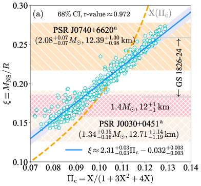
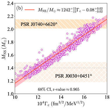
FIG. 1: (Color Online). Upper panel: The $\xi$-$\Pi_{\textrm{c}}$ correlation using meta-model EOSs consistent with observational/experimental constraints. The compactnesses for PSR J0740+6620 [12], PSR J0030+0451 [10] and the NS in the X-ray burster GS 1826-24 [18] are shown individually. The function $\mathrm{X}(\Pi_{\textrm{c}})$ is plotted by the dashed orange line and the compactness for a typical canonical NS [28, 17] (with $R\approx 12_{-1}^{+1}\,\textrm{km}$) by the hatched pink band. Lower panel: Same as panel (a) but for the correlation $M_{\textrm{NS}}$-$\Gamma_{\textrm{c}}$, the lavender and pink bands in panel (a) and (b) represents their 68% confidence intervals (CIs).

To test the compactness and mass scalings, we randomly generate $10^{5}$ meta-model EOSs. A NS meta-model is a model of models that can mimic all existing NS EOSs in the literature [1, 2, 3, 4], see the Supplementary Materials for a detailed description. To explore the whole EOS parameter space currently allowed and present our results clearly, we select randomly one point on each mass-radius (M-R) curve from a given EOS within the mass range of $1.2M_{\odot}\lesssim M_{\textrm{NS}}\lesssim 2.2M_{\odot}$. The resulting scalings are shown in FIG. 1. Here the panel (a) shows the compactness-$\Pi_{\textrm{c}}$ scaling while the panel (b) is the mass-$\Gamma_{\textrm{c}}$ scaling. In each panel, 500 representative samples are shown while $10^{5}$ EOSs are used in calculating the scaling coefficients and their error bands. The standard error (ste) and the coefficient of determination (the r-value) actually start converging quickly using about 300 samples. In particular, the ste for the compactness-$\Pi_{\textrm{c}}$ (mass-$\Gamma_{\textrm{c}}$) regression is about 0.03 (0.002$M_{\odot}$) and the r-value for both regressions is about 0.97. The regression and its 68% confidence interval (CI) are shown by the light-blue (tomato) line and lavender (pink) band, respectively. Quantitatively, we have $\xi\approx A_{\xi}\Pi_{\textrm{c}}+B_{\xi}\approx 2.31_{-0.03}^{+0.03}\Pi_{\textrm{c}}-0.032_{-0.003}^{+0.003}$ for the compactness-$\Pi_{\textrm{c}}$ scaling and $M_{\textrm{NS}}/M_{\odot}\approx A_{\textrm{M}}\Gamma_{\textrm{c}}+B_{\textrm{M}}\approx 1242_{-15}^{+15}\Gamma_{\textrm{c}}-0.08_{-0.02}^{+0.02}$ for the mass-$\Gamma_{\textrm{c}}$ scaling, respectively. Since $\mathrm{X}$ is limited to $\mathrm{X}\lesssim 0.374$ [55] by causality realized in General Relativity (GR) with strong-field gravity, we have $\xi\lesssim 0.264_{-0.005}^{+0.005}\equiv\xi_{\textrm{GR}}$ which is consistent with its upper bound of 0.33 extracted in Ref. [63]. We also analyzed the radius-$\nu_{\textrm{c}}$ correlation and obtained the scaling $R/\textrm{km}\approx A_{\textrm{R}}\nu_{\textrm{c}}+B_{\textrm{R}}\approx 572_{-25}^{+25}\nu_{\textrm{c}}+4.22_{-0.35}^{+0.35}$ with a r-value about 0.712 and the $R$-ste of about 0.3 km which is much smaller than that in current NS observations. As noticed earlier, dividing $R$ by $M_{\textrm{NS}}$ in calculating the compactness $\xi$ largely diminishes the relatively large uncertainty in the radius scaling. We thus use the $\xi$-$\Pi_{\textrm{c}}$ and $M_{\textrm{NS}}$-$\Gamma_{\textrm{c}}$ scalings in our following studies.

In panel (a) of FIG. 1, we show the compactnesses for PSR J0740+6620 and PSR J0030+0451 via NICER’s simultaneous mass-radius observation, namely $M_{\textrm{NS}}/M_{\odot}\approx 2.08_{-0.07}^{+0.07}$ and $R/\textrm{km}\approx 12.39_{-0.98}^{+1.30}$ (at 95% CI) for the former [12] and $M_{\textrm{NS}}/M_{\odot}\approx 1.34_{-0.16}^{+0.15}$ and $R/\textrm{km}\approx 12.71_{-1.19}^{+1.14}$ (at 68% CI) for the latter [10], both indicated by the superscript “a”. Shown also are the compactness $\xi\approx 0.183\sim 0.259$ for the NS in GS 1826-24 directly from its surface gravitational red-shift measurement [18] and the $\xi$ for a canonical NS with $R\approx 12_{-1}^{+1}\,\textrm{km}$ [28, 17]. For a given $\xi$, one can directly obtain the $\Pi_{\textrm{c}}$ from their scaling and the $\mathrm{X}$ via the function $\mathrm{X}(\Pi_{\textrm{c}})$ (orange dashed line) defined in Eq. (3).

Similarly, the mass bands for PSR J0740+6620 [44] and PSR J0030+0451 [10] are shown in panel (b). Giving a mass $M_{\textrm{NS}}$, the mass-$\Gamma_{\textrm{c}}$ scaling upper bounds the $\varepsilon_{\textrm{c}}$ allowed since $\mathrm{X}\lesssim 0.374$ [55]. For a canonical NS, this upper bound is about $\mathrm{Y}\equiv\varepsilon_{\textrm{c}}/\varepsilon_{0}\lesssim 9.9$ where $\varepsilon_{0}\approx 150\,\textrm{MeV}/\textrm{fm}^{3}$ denotes the energy density at nuclear saturation density $\rho_{0}$; while for a NS with $M_{\textrm{NS}}/M_{\odot}\approx 2.0$, we have $\mathrm{Y}\lesssim 5.0$.

Extracting NS Observational Constraints on Trace Anomalies Independent of EOS Models: The strong linear correlation between $\xi$ and $\Pi_{\textrm{c}}$ of Eq. (3) enables us to read off the $\mathrm{X}$ straightforwardly from the $\xi$ obtained either using NS mass-radius observation or the red-shift measurement; and therefore the central trace anomaly $\Delta_{\textrm{c}}=1/3-\mathrm{X}$. Since the ratio $P/\varepsilon$ increases towards NS centers and reaches its maximum value $\mathrm{X}$ there, the trace anomaly takes its minimum $\Delta_{\textrm{c}}$ there. A lower bound for trace anomaly $\Delta\gtrsim\Delta_{\textrm{GR}}\approx-0.041$ from the GR limit $\mathrm{X}\lesssim 0.374$ [55] is then equivalently to its limit $\xi\lesssim 0.264_{-0.005}^{+0.005}$ for the compactness discussed earlier.

In panel (a) of FIG. 2, we show the $\xi$-dependence of $\Delta_{\textrm{c}}$ by inverting $\xi\approx A_{\xi}\Pi_{\textrm{c}}(\mathrm{X})+B_{\xi}$ (pink band). Here 14 NS instances are shown, these include two alternative inferences of the radius using somewhat different approaches for PSR J0030+0451 [11] by superscript “a,b” and three for PSR J0740+6620 [13, 14] by “a,b,c”; the NS in GS 1826-24 [18], a canonical NS with radius $R\approx 12_{-1}^{+1}\,\textrm{km}$ [28]; and three central trace anomalies for PSR J2215+5135 [19]. Though there is currently no observational constraint on the radius of PSR J2215+5135, we can use the $\xi_{\textrm{GR}}$ or $\Delta_{\textrm{GR}}$ to limit $R\gtrsim 12\,\textrm{km}$. Here three typical radii, namely 12 km, 13 km and 14 km are adopted for an illustration. It is known that the two NSs involved in GW 170817 [15] have $R_{1}\approx R_{2}\approx 11.9_{-1.4}^{+1.4}\,\textrm{km}$ as well as $1.36\lesssim M_{\textrm{NS1}}/M_{\odot}\lesssim 1.58$ and $1.18\lesssim M_{\textrm{NS2}}/M_{\odot}\lesssim 1.36$, respectively; while GW 190425 [16] has $13.1\,\textrm{km}\lesssim R_{1}\lesssim 14.9\,\textrm{km}$ with $1.6\lesssim M_{\textrm{NS1}}/M_{\odot}\lesssim 1.9$ and $13.3\,\textrm{km}\lesssim R_{2}\lesssim 14.9\,\textrm{km}$ with $1.5\lesssim M_{\textrm{NS2}}/M_{\odot}\lesssim 1.7$, respectively, using the low-spin prior [65]. The error bar of $\Delta_{\textrm{c}}$ is mainly due to the uncertainty of $\xi$ itself as the correlation $\xi$-$\Pi_{\textrm{c}}$ is strong and model independent. For instance, the error bar of $\Delta_{\textrm{c}}$ for a canonical NS with $R\approx 12_{-1}^{+1}\,\textrm{km}$ is apparently smaller than that for the two NSs in GW 170817 [15] as they have larger mass uncertainties although they share similar radii (compare the red solid pentagon and dark-violet solid circles).

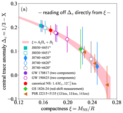
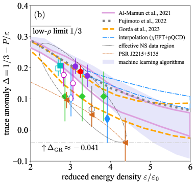
FIG. 2: (Color Online). Upper panel: Central trace anomaly $\Delta_{\textrm{c}}$ as a function of compactness $\xi$ from inverting the compactness scaling (pink band) in comparison with observational data indicated. Lower panel: Energy density dependence of the trace anomaly where the trace anomalies from a few empirical NS EOSs via different input data/inference algorithms are also given. The GR bound $\Delta\gtrsim\Delta_{\textrm{GR}}\approx-0.041$ is plotted by the grey dash-dotted line, see text for more details.

Besides the $\xi$-$\Pi_{\textrm{c}}$ scaling, the mass-$\Gamma_{\textrm{c}}$ scaling of Eq. (1) further gives individually the values of $P_{\textrm{c}}$ and $\varepsilon_{\textrm{c}}$ if both the $M_{\textrm{NS}}$ and $R$ (or one of them together with the compactness) are observationally known. In order to obtain $\mathrm{X}$ and $\varepsilon_{\textrm{c}}$ for the NS in GS 1826-24 (only its compactness is known), we adopt three typical radii (12 km, 13 km and 14 km), the same as that for PSR J2215+5135. See the Supplementary Materials for the numerical values of $\mathrm{X}$ and $\mathrm{Y}\equiv\varepsilon_{\textrm{c}}/\varepsilon_{0}$ for the 16 NS instances discussed above; they are also displayed in panel (b) of FIG. 2 and enclosed by the dotted black ellipse (effective region of NS data). For comparisons, also shown are the trace anomalies obtained/constrained by a few contemporary state-of-the-art NS EOS modelings using different input data and/or inference algorithms. These include the NS EOS inference [66] incorporating the pQCD impact (dashed orange band), a Bayesian inference of NS EOS [67] combining the electromagnetic and gravitational-wave signals (plum solid band), the interpolation [20] between low-density chiral effective field theories [26] ($\chi$EFT) and high-density pQCD constraints [68] (between the dash-dotted light-blue lines), a minimal parametrization [20] of $\Delta$ versus $\varepsilon/\varepsilon_{0}$ (grey dotted line) accounting for NS data and the NS EOS [20] inferred via machine learning algorithms (lavender band).

Our results of ($\mathrm{Y}\equiv\varepsilon_{\textrm{c}}/\varepsilon_{0}$, $\Delta_{\textrm{c}}=1/3-\mathrm{X})$ for the 16 NS instances put stringent constraints on the theoretical NS EOSs. As shown in panel (b) of FIG. 2, apparently the $\Delta$’s and especially their energy dependence (which determines the speed of sound as we shall discuss next) from some NS EOS modelings have sizable tensions with the limits set by the observational data based on our scaling analyses, especially for massive NSs. It implies that some ingredients in modeling NS EOS may need to be revised. For example, the NS EOS model incorporating pQCD effect [66] can well explain the $(\mathrm{Y},\Delta_{\textrm{c}})$’s of PSR J0030+0451, GW 190425 and GS 1826-24 (with a radius $R\approx 12\,\textrm{km}$, the rightest green diamond). However, it could hardly account for the results for PSR J0740+6620 for all three radii [12, 13, 14] and the two NSs in GW 170817 [15] as well as those for PSR J2215+5135 [19] (for all three $R$’s). Similarly, the NS EOS modeling with both the electromagnetic and gravitational-wave signals included [67] can effectively explain the data of GW 170817 and the canonical NS. But it has certain tensions with our results based on observations for PSR J0030+451 and PSR J0740+6620, GW 190425 and the redback spider pulsar PSR J2215+5135. Interestingly, although GW 190425 executes weaker limits on NS radii [16], it effectively puts useful constraints on the $\Delta$. On the other hand, the interpolation [20] between low-density $\chi$EFT [26] and high-density pQCD [68] predicts a quite large $\Delta$ compared with what we extracted from PSR J0740+6620, GS 1826-24 and PSR J2215+5135 observations.

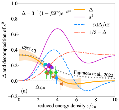
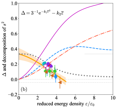
FIG. 3: (Color Online). The trace anomaly $\Delta$, $s^{2}$ and its decomposition via Eq. (4) using two effective parametrizations for $\Delta$. The 16 NS instances of panel (b) of FIG. 2 are plotted with the tan band for its 68% CI regression in each panel. The grey dotted line represents the minimal parametrization of Ref. [20].

Can We Extract a Peaked Speed of Sound Invariably from the Available NS Data? The trace anomaly $\Delta$ and its derivative with respect to energy density are crucial for understanding the speed of sound squared $s^{2}$ in NSs [20],

$$s^{2}\equiv\frac{\mathrm{d}P}{\mathrm{d}\varepsilon}=-\overline{\varepsilon}\frac{\mathrm{d}\Delta}{\mathrm{d}\overline{\varepsilon}}+\frac{1}{3}-\Delta,$$ (4)

where $\overline{\varepsilon}\equiv\varepsilon/\varepsilon_{0}$. The first term is obviously the derivative while the remainings together represent the non-derivative part of $s^{2}$. Panel (a) of FIG. 3 shows an effective parametrization $\Delta\approx 3^{-1}(1-ft\overline{\varepsilon}^{a})\exp(-t\overline{\varepsilon}^{a})$ as a function of $\overline{\varepsilon}$ to averagely account for the 16 NS instances, valid for $2.5\lesssim\overline{\varepsilon}\lesssim 4.5$ (data available). Here $a\approx 2.63$ and $t\approx 0.02$ are two parameters, and $f\equiv\textrm{L}_{W}(-3^{-1}/\textrm{e}\Delta_{\textrm{GR}})\approx 0.9539$ with $\textrm{L}_{W}(x)$ being the Lambert-$W$ function defined as the solution of the equation $w\exp(w)=x$. This parametrization has the following properties: (i) $\Delta\to 0$ for $\overline{\varepsilon}\to\infty$ [68], and (ii) $\Delta\to 1/3$ as $\overline{\varepsilon}\to 0$; it also generates a minimum $\Delta_{\min}=\Delta_{\textrm{GR}}\approx-0.041$ at $\overline{\varepsilon}_{\textrm{GR}}=[(f+1)/ft]^{1/a}\approx 5.8$ by construction (through the factor $f$). Due to these features especially the GR bound $\Delta_{\textrm{GR}}$, both a peak and a valley emerge in $s^{2}$ between $0<\overline{\varepsilon}_{\textrm{pk}}\approx 4<\overline{\varepsilon}_{\textrm{GR}}$ and at $\overline{\varepsilon}_{\textrm{vl}}\approx 7.2>\overline{\varepsilon}_{\textrm{GR}}$, respectively; though the latter energy density may not be reachable in realistic NSs. On the other hand, if we adopt another effective parametrization for $\Delta$ considering only the constraint $\lim_{\overline{\varepsilon}\to 0}\Delta=3^{-1}$ (without its large $\overline{\varepsilon}$-limit) but can describe the NS data approximately equally well as the previous one, e.g., $\Delta\approx 3^{-1}\exp[-k_{1}\overline{\varepsilon}^{2}]-k_{2}\overline{\varepsilon}$ with two parameters $k_{1}\approx 0.037$ and $k_{2}\approx 0.032$, the resulting $s^{2}$ just monotonically increase with $\overline{\varepsilon}$ in spite of the fact that a broad peak exists in the derivative term “$-\overline{\varepsilon}\mathrm{d}\Delta/\mathrm{d}\overline{\varepsilon}$”. A quantitative comparison of the two parameterizations and detailed analyses of their features are given in the Supplementary Materials.

The findings above demonstrate that a peaked shape of $s^{2}$ is an implication considering some well-founded theoretical limits but not practically inevitable, and it is not a direct consequence of the currently available NS data. As more observational data on mass, radius or red-shift becomes available, our approach based on NS compactness and mass scalings can better constrain the trace anomaly $\Delta$ in a wide range of energy densities, locate precisely the possible peak positions of $s^{2}$ relying on NS data alone without using other physical inputs [69], and restrict the NS EOS to a much narrower band.

Conclusions: Using a novel approach based on the predicted scaling of NS compactness with its central pressure/energy density ratio from perturbatively analyzing the dimensionless TOV equations that is also verified by $10^{5}$ meta-model EOSs, we have shown that NS central trace anomaly can be extracted reliably from its observational data directly independent of the EOS models. Using the available data on the mass, radius and/or compactness of several NSs from recent X-ray and gravitational wave observations we extracted the central trace anomaly as a function of energy density. It stringently tests the existing EOS models and sets a clear guidance in a new direction for further understanding the nature and EOS of supradense matter in a model-independent manner.

Acknowledgement: We would like to thank Wen-Jie Xie and Nai-Bo Zhang for helpful discussions. This work was supported in part by the U.S. Department of Energy, Office of Science, under Award Number DE-SC0013702, the CUSTIPEN (China-U.S. Theory Institute for Physics with Exotic Nuclei) under the US Department of Energy Grant No. DE-SC0009971.

Supplementary Materials

Unraveling Trace Anomaly of Supradense Matter

via Neutron Star Compactness Scaling

Bao-Jun Cai and Bao-An Li

I.  Meta-model Equation of State of Neutron Star Matter

We adopt a meta-model for generating randomly NS EOSs in a broad parameter space that can mimic diverse model predictions consistent will existing constraints from terrestrial experiments and astrophysical observations as well as general physics principles [1, 2, 3, 4]. It is based on a so-called minimum model of NSs consisting of neutrons, protons, electrons and muons (npe$\mu$ matter) at $\beta$-equilibrium. Its most basic input is the EOS of isospin-asymmetric nucleonic matter in the form of energy per nucleon $E(\rho,\delta)=E_{0}(\rho)+E_{\textrm{sym}}(\rho)\delta^{2}$, here $\rho=\rho_{\textrm{n}}+\rho_{\textrm{p}}$ and $\delta\equiv(\rho_{\textrm{n}}-\rho_{\textrm{p}})/(\rho_{\textrm{n}}+\rho_{\textrm{p}})$ is the isospin asymmetry of neutron-rich system with neutron density $\rho_{\textrm{n}}$ and proton density $\rho_{\textrm{p}}$, respectively. The EOS of symmetric nuclear matter $E_{0}(\rho)$ and the symmetry energy $E_{\textrm{sym}}(\rho)$ are parameterized respectively as $E_{0}(\rho)=B+2^{-1}K_{0}\chi^{2}+6^{-1}J_{0}\chi^{3}+24^{-1}I_{0}\chi^{4}$ and $E_{\textrm{sym}}(\rho)=S+L\chi+2^{-1}K_{\textrm{sym}}\chi^{2}+6^{-1}J_{\textrm{sym}}\chi^{3}$ with $\chi\equiv(\rho-\rho_{0})/3\rho_{0}$, $B\equiv E_{0}(\rho_{0})$ and $S\equiv E_{\textrm{sym}}(\rho_{0})$, therefore defining the coefficients $K_{0}$, $J_{0}$, $\cdots$.

The total energy density is $\varepsilon(\rho,\delta)=[E(\rho,\delta)+M_{\textrm{N}}]\rho+\varepsilon_{\ell}(\rho,\delta)$ where $M_{\textrm{N}}\approx 939\,\textrm{MeV}$ and $\varepsilon_{\ell}(\rho,\delta)$ is the energy density of leptons from an ideal Fermi gas model [5]. The pressure $P(\rho,\delta)$ is $P(\rho,\delta)=\rho^{2}\mathrm{d}[\varepsilon(\rho,\delta)/\rho]/\mathrm{d}\rho$. The density profile of isospin asymmetry $\delta(\rho)$ is obtained by solving the $\beta$-equilibrium condition $\mu_{\textrm{n}}-\mu_{\textrm{p}}=\mu_{\textrm{e}}=\mu_{\mu}\approx 4\delta E_{\textrm{sym}}(\rho)$ and the charge neutrality requirement $\rho_{\textrm{p}}=\rho_{\textrm{e}}+\rho_{\mu}$. Here the chemical potential $\mu_{i}$ for a particle $i$ is calculated from the energy density via $\mu_{i}=\partial\epsilon(\rho,\delta)/\partial\rho_{i}.$ With the $\delta(\rho)$ calculated consistently using the inputs given above, both the pressure $P(\rho,\delta(\rho))$ and energy density $\varepsilon(\rho,\delta(\rho))$ become barotropic, i.e., depend on the density $\rho$ only. The EOS in the form of $P(\varepsilon)$ can then be used in solving the TOV equations. The core-crust transition density $\rho_{\textrm{cc}}$ is determined self-consistently by the thermodynamic method [6, 7]; in the inner crust with densities between $\rho_{\textrm{cc}}$ and $\rho_{\textrm{out}}\approx 2.46\times 10^{-4}\,\textrm{fm}^{-3}$ corresponding to the neutron dripline we adopt the parametrized EOS $P=\alpha+\beta\varepsilon^{4/3}$ [8]; and for $\rho<\rho_{\textrm{out}}$ we adopt the Baym-Pethick-Sutherland (BPS) and the Feynman-Metropolis-Teller (FMT) EOSs [9].

In order for a broad verification of the scalings studied in this work, we select the saturation density $\rho_{0}$ to be $0.15\,\textrm{fm}^{-3}\lesssim\rho_{0}\lesssim 0.17\,\textrm{fm}^{-3}$, the binding energy in the range of $-17\,\textrm{MeV}\lesssim B\lesssim-15\,\textrm{MeV}$, the incompressibility for symmetric matter in $210\,\textrm{MeV}\lesssim K_{0}\lesssim 250\,\textrm{MeV}$; the skewness in $-400\,\textrm{MeV}\lesssim J_{0}\lesssim 0\,\textrm{MeV}$ and the kurtosis in $400\,\textrm{MeV}\lesssim I_{0}\lesssim 1200\,\textrm{MeV}$; for the symmetry energy we adopt $28\,\textrm{MeV}\lesssim S\lesssim 36\,\textrm{MeV}$, $30\,\textrm{MeV}\lesssim L\lesssim 90\,\textrm{MeV}$, $-300\,\textrm{MeV}\lesssim K_{\textrm{sym}}\lesssim 0\,\textrm{MeV}$ as well as $200\,\textrm{MeV}\lesssim J_{\textrm{sym}}\lesssim 1000\,\textrm{MeV}$. These parameters generated randomly within the specified uncertainty ranges are consistent with terrestrial experimental and contemporary astrophysical constraints, see, e.g., Ref. [1, 2, 3, 4] for more discussions and FIG. 4 for a few samples of the generated mass-radius curves.

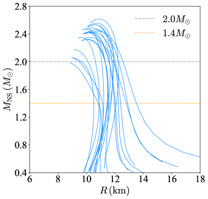
FIG. 4: Samples of the mass-radius curves generated by the meta-model NS EOSs.

II.  $\mathrm{X}$’s and $\mathrm{Y}$’s for the 16 NS Instances

We give the $\mathrm{X}$’s and $\mathrm{Y}$’s for the 16 NS Instances used in the main text in TAB. 1.

NS $\mathrm{X}\equiv P_{\textrm{c}}/\varepsilon_{\textrm{c}}$ $\mathrm{Y}\equiv\varepsilon_{\textrm{c}}/\varepsilon_{0}$   Ref. PSR J0030+0451${}^{\textrm{a}}$ $0.135_{-0.029}^{+0.025}$ $2.69_{-1.12}^{+1.07}$ [10] PSR J0030+0451${}^{\textrm{b}}$ $0.126_{-0.024}^{+0.026}$ $2.74_{-1.21}^{+1.25}$ [11] PSR J0740+6620${}^{\textrm{a}}$ $0.297_{-0.103}^{+0.077}$ $3.92_{-1.19}^{+0.90}$ [12] PSR J0740+6620${}^{\textrm{b}}$ $0.231_{-0.102}^{+0.058}$ $3.01_{-1.61}^{+0.93}$ [13] PSR J0740+6620${}^{\textrm{c}}$ $0.267_{-0.075}^{+0.057}$ $3.53_{-1.08}^{+0.84}$ [14] GW 170817 ($M_{\textrm{NS1}}$) $0.159_{-0.036}^{+0.036}$ $3.42_{-1.37}^{+1.37}$ [15] GW 170817 ($M_{\textrm{NS2}}$) $0.128_{-0.025}^{+0.025}$ $3.12_{-1.21}^{+1.21}$ [15] GW 190425 ($M_{\textrm{NS1}}$) $0.183_{-0.055}^{+0.055}$ $3.06_{-1.44}^{+1.44}$ [16] GW 190425 ($M_{\textrm{NS2}}$) $0.156_{-0.037}^{+0.037}$ $2.83_{-1.15}^{+1.15}$ [16] canonical NS $0.146_{-0.020}^{+0.020}$ $3.25_{-0.79}^{+0.79}$ [17] GS 1826-24 ($12\,\textrm{km}$) $0.226_{-0.082}^{+0.082}$ $3.83_{-2.16}^{+2.16}$ [18] GS 1826-24 ($13\,\textrm{km}$) $0.226_{-0.082}^{+0.082}$ $3.29_{-1.82}^{+1.82}$ [18] GS 1826-24 ($14\,\textrm{km}$) $0.226_{-0.082}^{+0.082}$ $2.86_{-1.61}^{+1.61}$ [18] PSR J2215+5135 ($12\,\textrm{km}$) $0.374_{-0.080}^{+0.080}$ $4.37_{-0.71}^{+0.71}$ [19] PSR J2215+5135 ($13\,\textrm{km}$) $0.283_{-0.039}^{+0.039}$ $3.53_{-0.57}^{+0.57}$ [19] PSR J2215+5135 ($14\,\textrm{km}$) $0.237_{-0.026}^{+0.026}$ $2.90_{-0.47}^{+0.47}$ [19]

TAB. 1: $\mathrm{X}=P_{\textrm{c}}/\varepsilon_{\textrm{c}}$ and $\mathrm{Y}\equiv\varepsilon_{\textrm{c}}/\varepsilon_{0}$ for the 16 NS instances, the central trace anomaly is $\Delta_{\textrm{c}}=1/3-\mathrm{X}$.

III.  Trace Anomaly $\Delta$, Speed of Sound Squared $s^{2}$ and its Decomposition within Effective Data Region

The $s^{2}$ in NSs can be decomposed in terms of the trace anomaly $\Delta$ and its derivative with respect to energy density as [20]

$$s^{2}=\underbrace{-\overline{\varepsilon}\frac{\mathrm{d}\Delta}{\mathrm{d}\overline{\varepsilon}}}_{s^{2}_{\textrm{deriv}}}+\underbrace{\frac{1}{3}-\Delta}_{s^{2}_{\textrm{non-deriv}}},~{}~{}\overline{\varepsilon}\equiv\varepsilon/\varepsilon_{0},$$ (5)

where the first term is the derivative part and the remaining terms together represent the non-derivative part. In the main text, two parametrizations for $\Delta$ are adopted for illustrations,

$$\mbox{parametrization (a)}:\Delta\approx 3^{-1}\left(1-ft\overline{\varepsilon}^{a}\right)\exp\left(-t\overline{\varepsilon}^{a}\right)$$

$$\approx 3^{-1}\left(1-0.9539t\overline{\varepsilon}^{a}\right)\exp\left(-t\overline{\varepsilon}^{a}\right),$$ (6)

$$\mbox{parametrization (b)}:\Delta\approx 3^{-1}\exp[{-k_{1}\overline{\varepsilon}^{2}}]-k_{2}\overline{\varepsilon},$$ (7)

here $a\approx 2.63$ and $t\approx 0.02$ as well as $k_{1}\approx 0.037$ and $k_{2}\approx 0.032$ are effective parameters estimated by the NS instances considered. Using them and the general formula (5), we can obtain the $s^{2}$ together with its decomposition, and the results are given in the main text. Numerically, we find $\Delta$ in panel (a) of Fig.3 in the main text drops most quickly at roughly about $\overline{\varepsilon}\approx 3.5$ from being $\gtrsim 0.1$ to $\lesssim 0.1$. This feature actually strongly connects with the possible peaked behavior of the squared sound speed [20]. The expected peak emerges at $\overline{\varepsilon}\approx 4$ or $\varepsilon\approx 600\,\textrm{MeV}/\textrm{fm}^{3}$ with $s^{2}\approx 0.67$; this is because $\Delta\to\Delta_{\textrm{GR}}$ somewhere and thus a peak emerges (at $\overline{\varepsilon}\approx 3.6$) in the derivative term “$-\overline{\varepsilon}\mathrm{d}\Delta/\mathrm{d}\overline{\varepsilon}$” [20]. So the peak position in $s^{2}$ is higher than that in $s_{\textrm{deriv}}^{2}$. More interestingly, the GR bound $\Delta_{\min}=\Delta_{\textrm{GR}}<0$ induces a valley in $s^{2}$ at $\overline{\varepsilon}\approx 7.2$ with $s^{2}\approx 0.23$, since $\Delta\to 0>\Delta_{\textrm{GR}}$ as $\varepsilon/\varepsilon_{0}\to\infty$ due to a valley appearing at about $\overline{\varepsilon}\approx 7.1$; however this density may exceed the one allowed in realistic NSs. In this sense, the pQCD limit for $\Delta$ is the origin for the emergence of a valley in $s^{2}$ instead of a peak [20]. It also shows that the valley position in $s^{2}$ is slightly above that in $s^{2}_{\textrm{deriv}}$. On the other hand, using the parametrization (7) which considers only the constraint $\lim_{\overline{\varepsilon}\to 0}\Delta=3^{-1}$ (without its large $\overline{\varepsilon}$-limit) and can describe the available NS data approximately equally well within about $2.5\lesssim\overline{\varepsilon}\lesssim 4.5$, the full $s^{2}$ simply increases monotonically with increasing $\overline{\varepsilon}$ in spite of the fact that a broad peak still exists in the derivative term “$-\overline{\varepsilon}\mathrm{d}\Delta/\mathrm{d}\overline{\varepsilon}$”. Specifically, we find the peak in the derivative part $-\overline{\varepsilon}\mathrm{d}\Delta/\mathrm{d}\overline{\varepsilon}$ occurs at $\overline{\varepsilon}\approx 6.2$ with full $s^{2}\approx 0.88$.

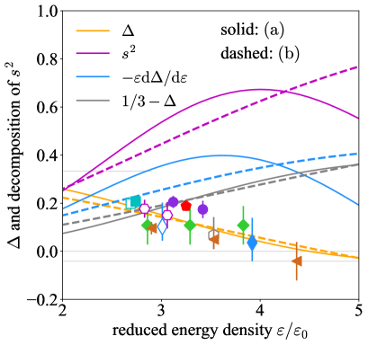
FIG. 5: (Color Online). Within the effective data region $2.5\lesssim\overline{\varepsilon}\lesssim 4.5$, the parametrization (6) and parametrization (7) for $\Delta$ behave very similarly.

FIG. 6: (Color Online). The trace anomaly $\Delta$ in the left panel may generate a peaked $s^{2}$ while that in the right panel implies $\mathrm{d}\Delta/\mathrm{d}\overline{\varepsilon}\approx\textrm{const.}<0$ and $s^{2}$ may thus increase monotonically with $\varepsilon/\varepsilon_{0}$. The solid line in each panel represents the probable shape of $\Delta$. Our scalings provide a useful tool to extract the $\Delta$ and $\varepsilon/\varepsilon_{0}$ directly from the observational data (masses, radii).

Within the effective data region in energy density, the parametrizations (a) and (b) behave very similarly and they are approximately equally accurate in describing the data, see FIG. 5. It means that the currently available NS mass and radius data could not tell whether there exists a peaked behavior in $s^{2}$. As more data on masses and radii or red-shifts becomes available, we will be able to distinguish whether a peaked $s^{2}$ may emerge. For an illustration, shown in FIG. 6 are two typical shapes of $\Delta$ versus $\varepsilon/\varepsilon_{0}$. In the left panel, we expect $s^{2}$ to have a peak somewhere since there is a quickly decreasing $\Delta$ between two approximate plateaus at low and high energy densities; while the $\Delta$ in the right panel indicates that $-\mathrm{d}\Delta/\mathrm{d}\overline{\varepsilon}$ is approximately positive and constant, both the derivative part $-\overline{\varepsilon}\mathrm{d}\Delta/\mathrm{d}\overline{\varepsilon}$ and the non-derivative term $1/3-\Delta$ may monotonically increase with $\varepsilon/\varepsilon_{0}$.

IV.  Understanding the Peaked/valleyed Behavior of $s^{2}$

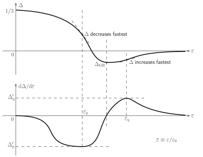
FIG. 7: Sketches of the trace anomaly $\Delta$ (upper panel) and its derivative $\mathrm{d}\Delta/\mathrm{d}\overline{\varepsilon}$ (lower panel) as functions of energy density.

The results of FIG. 3 in the main text could be understood by considering the general feature of the derivative term $\Delta^{\prime}\equiv\mathrm{d}\Delta/\mathrm{d}\overline{\varepsilon}$. There is a point $\overline{\varepsilon}_{\textrm{p}}$ in energy density where $\Delta$ decreases fastest; around this point-p we can expand $\Delta^{\prime}$ as

$$\Delta^{\prime}\approx\Delta_{\textrm{p}}^{\prime}+\frac{1}{2}\Delta_{\textrm{p}}^{\prime\prime\prime}\left(\overline{\varepsilon}-\overline{\varepsilon}_{\textrm{p}}\right)^{2},~{}~{}\Delta_{\textrm{p}}^{\prime}<0,~{}~{}\Delta_{\textrm{p}}^{\prime\prime\prime}>0,$$ (8)

since the first-order derivative of $\Delta^{\prime}$, namely $\Delta^{\prime\prime}$ at point-p is zero, see FIG. 7. Since $\Delta_{\textrm{p}}^{\prime\prime\prime}$ characterizes the curvature of $\Delta^{\prime}$, it is small for a shallow-shaped $\Delta^{\prime}$ but large for a sharp-shaped one. Correspondingly, the trace anomaly $\Delta$ itself around the point-p can be approximated by

$$\Delta\approx\Delta_{\textrm{p}}^{\prime}\left(\overline{\varepsilon}-\overline{\varepsilon}_{\textrm{p}}\right)+\frac{1}{6}\Delta_{\textrm{p}}^{\prime\prime\prime}\left(\overline{\varepsilon}-\overline{\varepsilon}_{\textrm{p}}\right)^{3}+\Delta_{\textrm{p}}.$$ (9)

Then we obtain the $s^{2}$ using the formula (5). Calculating the derivative $\mathrm{d}s^{2}/\mathrm{d}\overline{\varepsilon}$ gives

$$\frac{\mathrm{d}s^{2}}{\mathrm{d}\overline{\varepsilon}}=-2\Delta_{\textrm{p}}^{\prime}+\left(3\overline{\varepsilon}_{\textrm{p}}\overline{\varepsilon}-2\overline{\varepsilon}^{2}-\overline{\varepsilon}_{\textrm{p}}^{2}\right)\Delta_{\textrm{p}}^{\prime\prime\prime}.$$ (10)

We discuss it in the following two cases:

1. If the valley of the $\Delta^{\prime}$ curve is shallow, i.e., $\Delta_{\textrm{p}}^{\prime\prime\prime}$ is positively small, we can neglect the second term in (10),

   $$\frac{\mathrm{d}s^{2}}{\mathrm{d}\overline{\varepsilon}}\approx-2\Delta_{\textrm{p}}^{\prime}>0.$$ (11)

   This means that even when there exists a peak in $-\overline{\varepsilon}\mathrm{d}\Delta/\mathrm{d}\overline{\varepsilon}$ (equivalently a valley in $\mathrm{d}\Delta/\mathrm{d}\overline{\varepsilon}$), the $s^{2}$ is a monotonically increasing function of $\overline{\varepsilon}$. This corresponds to the panel (b) of FIG. 3 in the main text.

2. On the other hand, if $|\Delta_{\textrm{p}}^{\prime}|$ is smaller than $\Delta_{\textrm{p}}^{\prime\prime\prime}$, i.e., the valley in $\Delta^{\prime}$ is sharp, we can treat the first term in (5) as a perturbation and solve the equation $\mathrm{d}s^{2}/\mathrm{d}\overline{\varepsilon}=0$ for its extreme point $\overline{\varepsilon}_{\textrm{p}}^{\ast}$. The result is

   $$\overline{\varepsilon}_{\textrm{p}}^{\ast} = \frac{3\overline{\varepsilon}_{\textrm{p}}\Delta_{\textrm{p}}^{\prime\prime\prime}+\sqrt{\overline{\varepsilon}_{\textrm{p}}^{2}\Delta_{\textrm{p}}^{\prime\prime\prime 2}-16\Delta_{\textrm{p}}^{\prime}\Delta_{\textrm{p}}^{\prime\prime\prime}}}{4\Delta_{\textrm{p}}^{\prime\prime\prime}}$$ (12)

   $$\approx \overline{\varepsilon}_{\textrm{p}}\left(1-\frac{2}{\overline{\varepsilon}_{\textrm{p}}^{2}}\frac{\Delta_{\textrm{p}}^{\prime}}{\Delta_{\textrm{p}}^{\prime\prime\prime}}\right)>\overline{\varepsilon}_{\textrm{p}},~{}~{}\mbox{for small }\Delta_{\textrm{p}}^{\prime}.$$

   Moreover, we have

   $$s^{2}(\overline{\varepsilon}_{\textrm{p}}^{\ast})\approx \frac{1}{3}-\Delta_{\textrm{p}}-\overline{\varepsilon}_{\textrm{p}}\Delta_{\textrm{p}}^{\prime},$$ (13)

   $$\left.\frac{\mathrm{d}^{2}s^{2}}{\mathrm{d}\overline{\varepsilon}^{2}}\right|_{\overline{\varepsilon}_{\textrm{p}}^{\ast}}\approx \Delta_{\textrm{p}}^{\prime\prime\prime}\overline{\varepsilon}_{\textrm{p}}\left(\frac{8}{\overline{\varepsilon}_{\textrm{p}}^{2}}\frac{\Delta_{\textrm{p}}^{\prime}}{\Delta_{\textrm{p}}^{\prime\prime\prime}}-1\right)<0.$$ (14)

   The negativeness of the second-order derivative shows that it is a maximum point (peak) of $s^{2}$. The correction in the bracket of (12) is positive, this means that the peak in $s^{2}$ occurs on the right side of the peak in $-\overline{\varepsilon}\mathrm{d}\Delta/\mathrm{d}\overline{\varepsilon}$. This is the panel (a) of FIG. 3 in the main text. We can also evaluate the decomposition terms $s_{1}^{2}\equiv-\overline{\varepsilon}\mathrm{d}\Delta/\mathrm{d}\overline{\varepsilon}$ and $s_{2}^{2}\equiv 3^{-1}-\Delta$ of $s^{2}$ at $\overline{\varepsilon}_{\textrm{p}}^{\ast}$,

   $$s_{1}^{2}(\overline{\varepsilon}_{\textrm{p}}^{\ast})\approx-\overline{\varepsilon}_{\textrm{p}}\Delta_{\textrm{p}}^{\prime},~{}~{}s_{2}^{2}(\overline{\varepsilon}_{\textrm{p}}^{\ast})\approx\frac{1}{3}-\Delta_{\textrm{p}}.$$ (15)

   Therefore,

   $$\frac{s^{2}(\overline{\varepsilon}_{\textrm{p}}^{\ast})}{s_{1}^{2}(\overline{\varepsilon}_{\textrm{p}}^{\ast})}=1-\frac{3^{-1}-\Delta_{\textrm{p}}}{\overline{\varepsilon}_{\textrm{p}}\Delta_{\textrm{p}}^{\prime}}>1.$$ (16)

The analysis for the point-q in FIG. 7 where $\Delta^{\prime}$ is a maximum is totally parallel. In particular, there exists a valley in $s^{2}$,

$$\left.\frac{\mathrm{d}^{2}s^{2}}{\mathrm{d}\overline{\varepsilon}^{2}}\right|_{\overline{\varepsilon}_{\textrm{q}}^{\ast}}\approx\Delta_{\textrm{p}}^{\prime\prime\prime}\overline{\varepsilon}_{\textrm{q}}\left(\frac{8}{\overline{\varepsilon}_{\textrm{q}}^{2}}\frac{\Delta_{\textrm{q}}^{\prime}}{\Delta_{\textrm{q}}^{\prime\prime\prime}}-1\right)>0,$$ (17)

at

$$\overline{\varepsilon}_{\textrm{q}}^{\ast}\approx\overline{\varepsilon}_{\textrm{q}}\left(1-\frac{2}{\overline{\varepsilon}_{\textrm{q}}^{2}}\frac{\Delta_{\textrm{q}}^{\prime}}{\Delta_{\textrm{q}}^{\prime\prime\prime}}\right)>\overline{\varepsilon}_{\textrm{q}},$$ (18)

since

$$\Delta_{\textrm{q}}^{\prime}>0,~{}~{}\Delta_{\textrm{q}}^{\prime\prime\prime}<0.$$ (19)

This means that the valley in $s^{2}$ appears after that in its derivative part, consistent with the numerical results given in the last section. The new feature is that the valley in the derivative part is definitely negative,

$$s_{1}^{2}(\overline{\varepsilon}_{\textrm{q}}^{\ast})\approx-\overline{\varepsilon}_{\textrm{q}}\Delta_{\textrm{q}}^{\prime}<0,$$ (20)

see the dashed light-blue line in panel (a) of FIG. 3 in the main text. Considering $\mathrm{d}\Delta/\mathrm{d}\overline{\varepsilon}\to 0$ for large $\overline{\varepsilon}$, the $s^{2}$ finally approaches its asymptotic value determined by pQCD theories.

References

- [1] J. Walecka, Ann. Phys. 83, 491 (1974).
- [2] S. Chin, Ann. Phys. 108, 301 (1976).
- [3] B. Freedman and L. McLerran, Phys. Rev. D 16, 1130 (1977); 1147 (1977); 1169 (1977).
- [4] A. Akmal, V. Pandharipande, and D. Ravenhall, Phys. Rev. C 58, 1804 (1998).
- [5] J. Lattimer and M. Prakash, Astrophys. J. 550, 426 (2001).
- [6] M. Alford et al., Rev. Mod. Phys. 80, 1455 (2008).
- [7] B.A. Li, L.W. Chen, and C.M. Ko, Phys. Rep. 464, 113 (2008).
- [8] P. Bedaque and A. Steiner, Phys. Rev. Lett. 114, 031103 (2015).
- [9] I. Tews et al., Astrophys. J. 860, 149 (2018).
- [10] L. McLerran and S. Reddy, Phys. Rev. Lett. 122, 122701 (2019).
- [11] G. Baym et al., Astrophys. J. 885, 42 (2019).
- [12] T.Q. Zhao and J. Lattimer, Phys. Rev. D 102, 023021 (2020).
- [13] H. Tan et al., Phys. Rev. Lett. 128, 161101 (2022).
- [14] H. Tan et al., Phys. Rev. D 105, 023018 (2022).
- [15] S. Altiparmak, C. Ecker, and L. Rezzolla, Astrophys. J. Lett. 939, L34 (2022).
- [16] C. Drischler, S. Han, and S. Reddy, Phys. Rev. C 105, 035808 (2022).
- [17] Y.J. Huang et al., Phys. Rev. Lett. 129, 181101 (2022).
- [18] C. Ecker and L. Rezzolla, Astrophys. J. Lett. 939, L35 (2022).
- [19] R. Somasundaram, I. Tews, and J. Margueron, Phys. Rev. C 107, 025801 (2023).
- [20] C. Providncia et al., arXiv:2307.05086 (2023).
- [21] E. Annala et al., Phys. Rev. Lett. 120, 172703 (2018).
- [22] E. Annala et al., Nat. Comm. 14, 8451 (2023).
- [23] N.B. Zhang and B.A. Li, Eur. Phys. J. A 59, 86 (2023).
- [24] Z. Cao and L.W. Chen, arXiv:2308.16783 (2023).
- [25] D. Mroczek et al., arXiv:2309.02345 (2023).
- [26] R. Essick et al., Phys. Rev. Lett. 127, 192701 (2021).
- [27] L. Brandes, W. Weise, and N. Kaiser, Phys. Rev. D 107, 014011 (2023).
- [28] L. Brandes, W. Weise, and N. Kaiser, Phys. Rev. D 108, 094014 (2023).
- [29] J. Takatsy et al., Phys. Rev. D 108, 043002 (2023).
- [30] P. Pang et al., Phys. Rev. C 109, 025807 (2024).
- [31] Y.Z. Fan et al., Phys. Rev. D 109, 043502 (2024).
- [32] D. Oliinychenko et al., Phys. Rev. C 108, 034908 (2023).
- [33] A. Watts et al., Rev. Mod. Phys. 88, 021001 (2016).
- [34] M. Oertel et al., Rev. Mod. Phys. 89, 015007 (2017).
- [35] G. Baym et al., Rep. Prog. Phys. 81, 056902 (2018).
- [36] I. Vidaa, Proc. Roy. Soc. Lond. A 474, 0145 (2018).
- [37] B.A. Li et al., Universe 7, 182 (2021).
- [38] C. Drischler, J. Holt, and C. Wellenhofer, Annu. Rev. Nucl. Part. Sci. 71, 403 (2021).
- [39] A. Lovato et al., arXiv:2211.02224 (2022).
- [40] A. Sorensen et al., Prog. Part. Nucl. Phys. 134, 104080 (2024).
- [41] Y. Fujimoto et al., Phys. Rev. Lett. 129, 252702 (2022).
- [42] T. Riley et al., Astrophys. J. Lett. 887, L21 (2019).
- [43] M. Miller et al., Astrophys. J. Lett. 887, L24 (2019).
- [44] E. Fonseca et al., Astrophys. J. Lett. 915, L12 (2021).
- [45] T. Riley et al., Astrophys. J. Lett. 918, L27 (2021).
- [46] M. Miller et al., Astrophys. J. Lett. 918, L28 (2021).
- [47] T. Salmi et al., Astrophys. J. 941, 150 (2022).
- [48] X. Zhou et al., Nat. Phys. 1477, 69 (2023).
- [49] B. Abbott et al., Phys. Rev. Lett. 119, 161101 (2017).
- [50] B. Abbott et al., Phys. Rev. Lett. 121, 161101 (2018).
- [51] B. Abbott et al., Astrophys. J. Lett. 892, L3 (2020).
- [52] A. Sullivan and R. Romani, arXiv:2405.13889 (2024).
- [53] R. Tolman, Phys. Rev. 55, 364 (1939).
- [54] J. Oppenheimer and G. Volkoff, Phys. Rev. 55, 374 (1939).
- [55] B.J. Cai, B.A. Li, and Z. Zhang, Astrophys. J. 952, 147 (2023).
- [56] B.J. Cai, B.A. Li, and Z. Zhang, Phys. Rev. D 108, 103041 (2023).
- [57] B.J. Cai and B.A. Li, Phys. Rev. D 109, 083015 (2024).
- [58] J. Lattimer, slide 15, talk given at the 60th International Winter Meeting in Nuclear Physics, Jan. 22-26, 2024, Bormio, Italy.
- [59] N.B. Zhang, B.A. Li, and J. Xu, Astrophys. J. 859, 90 (2018)
- [60] N.B. Zhang and B.A. Li, Astrophys. J. 879, 99 (2019).
- [61] W.J. Xie and B.A. Li, Astrophys. J. 899, 4 (2020).
- [62] N.B. Zhang and B.A. Li, Astrophys. J. 921, 111 (2021).
- [63] E. Annala et al., Phys. Rev. X 12, 011058 (2022).
- [64] J. Richter and B.A. Li, Phys. Rev. C 108, 055803 (2023).
- [65] B. Abbott et al., Phys. Rev. X 11, 021053 (2021).
- [66] T. Gorda, O. Komoltsev, and A. Kurkela, Astrophys. J. 950, 107 (2023).
- [67] M. Al-Mamun et al., Phys. Rev. Lett. 126, 061101 (2021).
- [68] J. Bjorken, Phys. Rev. D 27, 140 (1983).
- [69] D. Zhou, arXiv:2307.11125 (2023).

References

- [1] N.B. Zhang, B.A. Li, and J. Xu, Astrophys. J. 859, 90 (2018).
- [2] N.B. Zhang and B.A. Li, Astrophys. J. 879, 99 (2019).
- [3] W.J. Xie and B.A. Li, Astrophys. J. 899, 4 (2020).
- [4] N.B. Zhang and B.A. Li, Astrophys. J. 921, 111 (2021).
- [5] J. Oppenheimer and G. Volkoff, Phys. Rev. 55, 374 (1939).
- [6] J. Lattimer and M. Prakash, Phys. Rep. 442, 109 (2007).
- [7] J. Xu et al., Astrophys. J. 697, 1549 (2009).
- [8] K. Iida and K. Sato, Astrophys. J. 477, 294 (1997).
- [9] G. Baym, C. Pethick, and P. Sutherland, Astrophys. J. 170, 299 (1971).
- [10] T. Riley et al., Astrophys. J. Lett. 887, L21 (2019).
- [11] M. Miller et al., Astrophys. J. Lett. 887, L24 (2019).
- [12] T. Riley et al., Astrophys. J. Lett. 918, L27 (2021).
- [13] M. Miller et al., Astrophys. J. Lett. 918, L28 (2021).
- [14] T. Salmi et al., Astrophys. J. 941, 150 (2022).
- [15] B. Abbott et al., Phys. Rev. Lett. 121, 161101 (2018).
- [16] B. Abbott et al., Astrophys. J. Lett. 892, L3 (2020).
- [17] J. Richter and B.A. Li, Phys. Rev. C 108, 055803 (2023).
- [18] X. Zhou et al., Nat. Phys. 1477, 69 (2023).
- [19] A. Sullivan and R. Romani, arXiv:2405.13889 (2024).
- [20] Y. Fujimoto et al., Phys. Rev. Lett. 129, 252702 (2022).