Nonlinear effects on charge fractionalization in critical chains
Abstract
We investigate the generic transport in a one-dimensional strongly correlated fermionic chain beyond linear response. Starting from a Gaussian wave packet with positive momentum on top of the ground state, we find that the numerical time evolution splits the signal into at least three distinct fractional charges moving with different velocities. A fractional left-moving charge is expected from conventional Luttinger liquid theory, but for the prediction of the two separate right-moving packets the nonlinearity of the dispersion must also be taken into account. This out-of-equilibrium protocol therefore allows a direct measurement of nonlinear interaction parameters, which also govern threshold singularities of dynamic response functions. The nonlinear Luttinger Liquid theory also predicts the correct dynamics at low energies, where it agrees with the conventional Luttinger liquid. Moreover, at high energies, the wave packet dynamics reveals signatures of composite excitations containing two-particle bound states. Our results uncover a simple strategy to probe the nonlinear regime in time-resolved experiments in quantum wires and ultracold-atom platforms.
Introduction.— The fractionalization of a particle into a composite of emergent excitations is one of the most striking phenomena in quantum many-body systems. The effect is prevalent in critical one-dimensional (1D) systems, in which interactions inevitably lead to a departure from Fermi liquid behavior Giamarchi (2004); Haldane (1981); Deshpande et al. (2010). Within the paradigm of Luttinger liquid (LL) theory Tomonaga (1950); Luttinger (1963), the low-energy spectrum of 1D quantum fluids is described by bosonic collective modes with a linear dispersion relation. This theory predicts that electrons fractionalize into right- and left-moving excitations that carry interaction-dependent charges Pham et al. (2000); Leinaas et al. (2009), as indeed observed in transport experiments in quantum wires Steinberg et al. (2007); Le Hur et al. (2008); Kamata et al. (2014); Freulon et al. (2015). In addition, signatures of LL behavior have been identified via spectroscopic techniques Kim et al. (1996); Segovia et al. (1999); Auslaender et al. (2002, 2005); Kim et al. (2006); Mourigal et al. (2013) and quantum simulations in ultracold-atom platforms Kinoshita et al. (2004); Paredes et al. (2004); Pagano et al. (2014); Hilker et al. (2017).
Despite its impressive success, LL theory breaks down whenever finite-energy excitations and band curvature have to be taken into account Imambekov et al. (2012). To treat the effects of a nonlinear dispersion, more general techniques have been developed into what became known as the nonlinear Luttinger liquid (nLL) theory Rozhkov (2005); Pustilnik et al. (2006); Khodas et al. (2007); Imambekov and Glazman (2009); Pereira et al. (2008). In particular, dynamic response functions exhibit characteristic threshold singularities that can be described by treating the modes with finite energy and momentum as mobile impurities coupled to the gapless modes Pustilnik et al. (2006). The exponents associated with these singularities can be expressed in terms of scattering phase shifts and calculated exactly for integrable models Pereira et al. (2008); Cheianov and Pustilnik (2008); Imambekov and Glazman (2008); Essler (2010). In the time domain, the contributions from high-energy modes give rise to power-law-decaying temporal oscillations that dominate the long-time behavior Pereira (2012). Moreover, nonlinearities are predicted to lead to shock waves in the evolution of density and magnetization pulses Bettelheim et al. (2006); Bettelheim and Glazman (2012); Protopopov et al. (2013, 2014).
While the nonlinear regime is accessible in experiments Barak et al. (2010); Jin et al. (2019); Wang et al. (2020); Senaratne et al. (2022), direct tests of the threshold singularities predicted by nLL theory are hindered by the limited energy resolution or disorder-induced broadening of spectroscopic probes. In this work, we show that the effects of the high-energy excitation in nLL theory can be directly observed in an out-of-equilibrium protocol. We create a Gaussian wave packet with preselected momentum in a critical fermionic chain and simulate its evolution using the adaptive time-dependent density matrix renormalization group (tDMRG) White and Feiguin (2004). Similar protocols have been used to demonstrate fractionalization and spin-charge separation in the low-energy regime Jagla et al. (1993); Trauzettel et al. (2004); Kollath et al. (2005); Ulbricht and Schmitteckert (2009); Al-Hassanieh et al. (2013); Acciai et al. (2017); Scopa et al. (2021). Beyond the LL paradigm, the nonlinear dispersion leads to a splitting of the initial wave packet into three density humps that propagate with different velocities Moreno et al. (2013); Dontsov and Dmitriev (2021). Here, we show that the time-evolved signal can be predicted by nLL theory, which in turn provides a quantitative measurement of the interaction between the high-energy particle and the low-energy modes. At lower fillings and higher energies, we discover fingerprints of two-particle bound states in the wave packet dynamics.
Model and protocol.— We consider a spinless fermion model described by the Hamiltonian
| (1) |
where annihilates a fermion at site of a chain with sites, is the strength of the nearest-neighbor interaction, and is the local density operator. We work at fixed number of fermions , with average density . For , the Hamiltonian can be diagonalized as , where is the dispersion relation of free fermions with momentum , with lattice spacing set to unity. The ground state in this case is constructed by occupying single-particle states up to the Fermi momentum . More generally, the model in Eq. (1) is equivalent to the spin-1/2 XXZ chain and is exactly solvable via Bethe ansatz (BA) Korepin et al. (1993). We focus on the parameter regime , where the ground state of Eq. (1) is in a gapless phase described at low energies by LL theory Giamarchi (2004).
We prepare an initial state given by
| (2) |
corresponding to a Gaussian wave packet centered at , with variance in real space and mean momentum ; here, is a normalization constant. To add a particle with well-defined momentum, we choose with momentum uncertainty ; see Fig. 1(a). After the unitary evolution , we measure the time-dependent local charge excess defined as
| (3) |
Free fermions.— The local charge excess can be calculated exactly in the noninteracting case. For a finite chain with open boundary conditions, we obtain
| (4) |
where and with . The result is analogous to the evolution of a Gaussian wave packet in the single-particle problem Shankar (1994). For small , we can expand the dispersion as , where is the group velocity and is the effective mass for momentum . As a consequence, we observe a single packet that moves to the right with velocity and width growing as
| (5) |
We have used Eq. (4) to benchmark our tDMRG results, obtaining excellent agreement; see the Supplemental Material (SM) SM . In all the numerics henceforth, we set , , and . We keep up to 400 states per DMRG block and use the Trotter step . The largest truncation error is of order . The maximum time is set by stopping the simulations before the wave packets reach the chain boundaries.
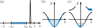
nLL theory.—We now turn to the interacting case. We seek to describe the dynamics using the framework of nLL theory Imambekov et al. (2012). In addition to the momentum , we consider a mode expansion that includes the low-energy modes in the vicinity of the Fermi points [see Fig. 1(b)]:
| (6) |
In the absence of the high-energy particle created by , the low-energy modes are described by the LL Hamiltonian Giamarchi (2004)
| (7) |
where is the velocity of the low-energy modes and are the right- and left-moving components of the bosonic field obeying
| (8) |
The low-energy fermion fields can be bosonized in the form
| (9) |
where is the Luttinger parameter. Taking the continuum limit of Eq. (1) including the high-energy mode, we obtain the effective Hamiltonian
| (10) |
where and are the renormalized energy and velocity, respectively, of the high-energy particle in the interacting model. Note that the high-energy particle behaves as a mobile impurity Tsukamoto et al. (1998); Balents (2000) that interacts with the bosonic modes via the coupling constants .
The impurity mode can be decoupled from the bosonic fields by the unitary transformation , where are the right- and left-mover phase shifts. In the nLL, govern all the space-time correlation functions of the system as well as the threshold singularities of dynamic response functions Pustilnik et al. (2006); Pereira et al. (2008). As we will see below, these non-trivial interaction parameters can be measured as fractional charges in our proposed out-of-equilibrium protocol.
We now proceed to calculate the fractional transport properties using the nLL theory. Up to irrelevant terms, the transformed Hamiltonian becomes noninteracting Pereira et al. (2009)
| (11) |
with
| (12) | |||||
| (13) |
Note that an initial excitation now consists of three parts: two vertex operators, , that excite low-energy modes propagating with velocity and a free particle with velocity , as schematically depicted in Fig. 1(b). The fractional charges of the three propagating parts can be measured with the charge density operator, which after rotation using Eq. (12) is given by
| (14) |
By calculating the commutator using Eq. (8), we have
| (15) |
Thus, the right- and left-moving vertex operators carry fractional charges propagating with velocity . The remaining charge corresponding to the particle is with velocity .
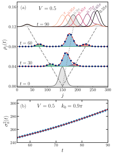
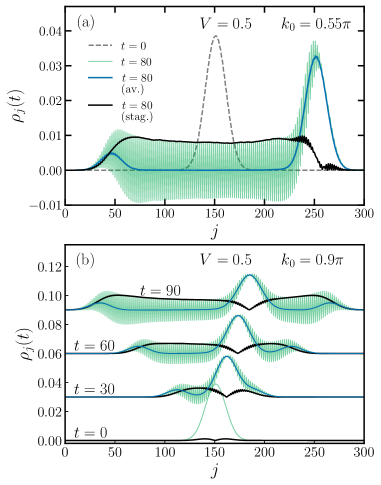
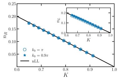
In the tDMRG simulation, we use the Gaussian wave packet defined in Eq. (2); see Fig. 1(a). The propagation at half-filling, , is shown in Fig. 2(a). Note that all parameters are known in this case: , , and momentum-independent phase shifts Pereira et al. (2008). In all cases, we observe three fractional humps that move with the exact velocities and magnitudes predicted by the nLL theory. Remarkably, the shape of the low-energy wave packets is stable over the whole energy regime, showing coherence over long times as it can be seen in Fig. 2(a). In addition, the variance of the high-energy hump, , grows in time according to Eq. (5) with an interaction-dependent effective mass; see Fig. 2(b). Therefore, the theoretical ad-hoc prediction of exactly three parts in the mode expansion (6) surprisingly provides a robust prediction of a free stable fractional particle. See the SM SM for more details on the fitting procedure.
Here, spatial oscillations in the density with wave number have been averaged out by taking the average between two nearest-neighbor sites. They can be attributed to the staggered part of the density operator as discussed in the SM SM .
In our analysis, we have used a large set of different values of , , and , which all show excellent agreement with the nLL theory. This implies that the nLL theory remarkably describes the whole energy regime covered by the Gaussian excitation with momentum . As predicted, we have not seen any momentum dependence in SM . Moreover, we observe a left-right symmetry in the low-energy humps, which is surprising since the initial wave packet at finite clearly does not have this symmetry. Last but not least, we can apply the theory also to excitations very close to the Fermi energy, i.e. . Once , longer and longer times are required to distinguish the two right-moving humps. In fact, this is in perfect agreement with conventional LL theory Pham et al. (2000) of only one left- and one right-moving fractional charge with and , respectively Pham et al. (2000). Hence, the continuous crossover from nLL to LL behavior becomes very intuitive in the dynamics of fractional charges . In contrast, this crossover is much more involved in the frequency domain since the threshold exponents are quadratic functions of the phase shifts Imambekov and Glazman (2009).
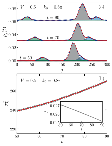
Quarter filling.—To illustrate a more generic situation, we now consider the model in Eq. (1) at quarter filling, . In this case, by solving Bethe ansatz equations, we can numerically determine the exact renormalized dispersion, Luttinger parameter, and velocity of the low-energy modes Giamarchi (2004); Korepin et al. (1993).
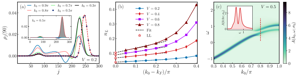
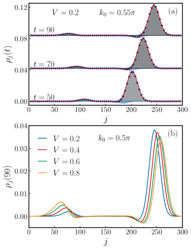
Figure 3(a) shows tDMRG results for and different values of at after averaging the density over four neighboring sites to smooth the oscillations out. In the low-energy regime, e.g. for , we observe only one left and one right hump moving with velocities , similar to the half-filled case. However, now the charge carried by the left-moving hump varies with as shown in Fig. 3(b), which in turn directly provides the momentum-dependent phase shifts . In the extrapolation we recover the LL prediction .
For larger values of , see for example and in Fig. 3(a), the three signals predicted by the nLL are observed again: two counter-propagating charges moving with velocities , and a large right-moving hump with velocity . Note that the right low-energy mover carries negative charge since . We again find that the time evolution of the excitation can be predicted by three propagating Gaussian wave packets SM .
As we increase the momentum, the density profile develops a complex pattern. For in Fig. 3(a), the broad feature around the middle of the chain suggests the presence of additional excitations. In fact, the operator in Eq. (2) can create not only individual particles but also composite excitations with net charge +1. To analyze the excitations, we consider the Fourier transform of the overlap between the initial state in Eq. (2) and the time-evolved one
| (16) |
where are eigenstates of with energy above the ground-state energy . In the limit , it reduces to the standard single-particle spectral function Pereira et al. (2009). We compute by performing a fast Fourier transform with a cosine window in the interval , with .
As discussed in Ref. [Pereira et al., 2009], the nLL theory for predicts a diverging peak at the dispersion , which decays as power laws on both sides with exponents dependent on the phase shifts. In our results of , this is reflected as a broad single-particle peak for ; see Fig. 3(c). At larger momenta, displays a double-peak structure for near , which is a clear indication of a yet unaccounted excitation in the wave packet in Eq. (LABEL:specd). This feature is absent for half-filling SM .
We identify this excitation as a composite of a two-particle bound state with a free hole as depicted in Fig. 1(c), which has been predicted in Ref. Pereira et al. (2009). Such a composite gives a high-energy continuum in the spectral function for momenta greater than , where restricts the momentum of bound state . Note that vanishes for or . In nLL theory, this type of excitation can be described by Pereira et al. (2009). For in Fig. 3(a), both the bound state () and the hole () are created near the bottom of their respective bands. This implies a low velocity, consistent with a slow-moving hump. In general, the evolution of the wave packet may involve contributions from low- or high-energy particles, holes, and bound states that share the total momentum covered by the Gaussian distribution; see the SM SM .
Conclusions.— We proposed an out-of-equilibrium protocol to investigate the fractionalization of high-energy excitations in critical chains. We clarified the crossover between LL and nLL regimes and identified contributions from elementary particles moving with different velocities and carrying fractional charges, which can be negative for . The transport simulations reveal also more involved excitations, such composite exctiations formed by holes and bound states. This analysis also applies to quantum spin chains and spin-charge separated quantum fluids Schmidt et al. (2010); Essler et al. (2015). Our work paves the way for precision tests of nLL effects through non-equilibrium dynamics in ultracold-atom platforms Pedersen et al. (2013); Vijayan et al. (2020) and time-resolved measurements of hot electrons in quantum wires and quantum Hall edge states Kataoka et al. (2016); Hashisaka et al. (2017); Bäuerle et al. (2018). In particular, we find a fractionally charged particle with free-particle dynamics, a right-moving low-energy excitation which can be negatively charged, and a left-moving signal that gives an exact measurement of the interaction couplings in a large parameter regime. Hence, experimental measurements of counter-propagating fractional charges directly provide quantitative values of the momentum-dependent interactions in the linear and the nonlinear regimes.
Acknowledgements.
This work was supported by the Deutsche Forschungsgemeinschaft (DFG, German Research Foundation) - Project No. 277625399-TRR 185 OSCAR (A4,A5), by the Conselho Nacional de Desenvolvimento Científico e Tecnológico (R.G.P.), and by a grant from the Simons Foundation (Grant No. 1023171, R.G.P.). The authors thank the high-performance cluster Elwetritsch for providing computational resources.References
- Giamarchi (2004) T. Giamarchi, Quantum physics in one dimension (Clarendon Press, Oxford, 2004).
- Haldane (1981) F. D. M. Haldane, ‘Luttinger liquid theory’ of one-dimensional quantum fluids. I. Properties of the Luttinger model and their extension to the general 1D interacting spinless Fermi gas, J. Phys. C 14, 2585 (1981).
- Deshpande et al. (2010) V. V. Deshpande, M. Bockrath, L. I. Glazman, and A. Yacoby, Electron liquids and solids in one dimension, Nature 464, 209 (2010).
- Tomonaga (1950) S. Tomonaga, Remarks on Bloch’s Method of Sound Waves applied to Many-Fermion Problems, Prog. Theor. Phys. 5, 544 (1950).
- Luttinger (1963) J. M. Luttinger, An Exactly Soluble Model of a Many-Fermion System, J. Math. Phys. 4, 1154 (1963).
- Pham et al. (2000) K.-V. Pham, M. Gabay, and P. Lederer, Fractional excitations in the Luttinger liquid, Phys. Rev. B 61, 16397 (2000).
- Leinaas et al. (2009) J. M. Leinaas, M. Horsdal, and T. H. Hansson, Sharp fractional charges in Luttinger liquids, Phys. Rev. B 80, 115327 (2009).
- Steinberg et al. (2007) H. Steinberg, G. Barak, A. Yacoby, L. N. Pfeiffer, K. W. West, B. I. Halperin, and K. L. Hur, Charge fractionalization in quantum wires, Nat. Phys. 4, 116 (2007).
- Le Hur et al. (2008) K. Le Hur, B. I. Halperin, and A. Yacoby, Charge fractionalization in nonchiral Luttinger systems, Ann. Phys. (N. Y.) 323, 3037 (2008).
- Kamata et al. (2014) H. Kamata, N. Kumada, M. Hashisaka, K. Muraki, and T. Fujisawa, Fractionalized wave packets from an artificial Tomonaga–Luttinger liquid, Nat. Nanotechnol. 9, 177 (2014).
- Freulon et al. (2015) V. Freulon, A. Marguerite, J. M. Berroir, B. Plaçais, A. Cavanna, Y. Jin, and G. Fève, Hong-Ou-Mandel experiment for temporal investigation of single-electron fractionalization, Nat. Commun. 6, 6854 (2015).
- Kim et al. (1996) C. Kim, A. Y. Matsuura, Z.-X. Shen, N. Motoyama, H. Eisaki, S. Uchida, T. Tohyama, and S. Maekawa, Observation of Spin-Charge Separation in One-Dimensional SrCu, Phys. Rev. Lett. 77, 4054 (1996).
- Segovia et al. (1999) P. Segovia, D. Purdie, M. Hengsberger, and Y. Baer, Observation of spin and charge collective modes in one-dimensional metallic chains, Nature 402, 504 (1999).
- Auslaender et al. (2002) O. M. Auslaender, A. Yacoby, R. de Picciotto, K. W. Baldwin, L. N. Pfeiffer, and K. W. West, Tunneling Spectroscopy of the Elementary Excitations in a One-Dimensional Wire, Science 295, 825 (2002).
- Auslaender et al. (2005) O. M. Auslaender, H. Steinberg, A. Yacoby, Y. Tserkovnyak, B. I. Halperin, K. W. Baldwin, L. N. Pfeiffer, and K. W. West, Spin-Charge Separation and Localization in One Dimension, Science 308, 88 (2005).
- Kim et al. (2006) B. J. Kim, H. Koh, E. Rotenberg, S.-J. Oh, H. Eisaki, N. Motoyama, S. Uchida, T. Tohyama, S. Maekawa, Z.-X. Shen, and C. Kim, Distinct spinon and holon dispersions in photoemission spectral functions from one-dimensional SrCuO2, Nat. Phys. 2, 397 (2006).
- Mourigal et al. (2013) M. Mourigal, M. Enderle, A. Klöpperpieper, J.-S. Caux, A. Stunault, and H. M. Rønnow, Fractional spinon excitations in the quantum Heisenberg antiferromagnetic chain, Nat. Phys. 9, 435 (2013).
- Kinoshita et al. (2004) T. Kinoshita, T. Wenger, and D. S. Weiss, Observation of a One-Dimensional Tonks-Girardeau Gas, Science 305, 1125 (2004).
- Paredes et al. (2004) B. Paredes, A. Widera, V. Murg, O. Mandel, S. Fölling, I. Cirac, G. V. Shlyapnikov, T. W. Hänsch, and I. Bloch, Tonks-Girardeau gas of ultracold atoms in an optical lattice, Nature 429, 277 (2004).
- Pagano et al. (2014) G. Pagano, M. Mancini, G. Cappellini, P. Lombardi, F. Schäfer, H. Hu, X.-J. Liu, J. Catani, C. Sias, M. Inguscio, and L. Fallani, A one-dimensional liquid of fermions with tunable spin, Nat. Phys. 10, 198 (2014).
- Hilker et al. (2017) T. A. Hilker, G. Salomon, F. Grusdt, A. Omran, M. Boll, E. Demler, I. Bloch, and C. Gross, Revealing hidden antiferromagnetic correlations in doped Hubbard chains via string correlators, Science 357, 484 (2017).
- Imambekov et al. (2012) A. Imambekov, T. L. Schmidt, and L. I. Glazman, One-dimensional quantum liquids: Beyond the Luttinger liquid paradigm, Rev. Mod. Phys. 84, 1253 (2012).
- Rozhkov (2005) A. V. Rozhkov, Fermionic quasiparticle representation of Tomonaga-Luttinger Hamiltonian, Eur. Phys. J. B 47, 193 (2005).
- Pustilnik et al. (2006) M. Pustilnik, M. Khodas, A. Kamenev, and L. I. Glazman, Dynamic Response of One-Dimensional Interacting Fermions, Phys. Rev. Lett. 96, 196405 (2006).
- Khodas et al. (2007) M. Khodas, M. Pustilnik, A. Kamenev, and L. I. Glazman, Fermi-Luttinger liquid: Spectral function of interacting one-dimensional fermions, Phys. Rev. B 76, 155402 (2007).
- Imambekov and Glazman (2009) A. Imambekov and L. I. Glazman, Universal Theory of Nonlinear Luttinger Liquids, Science 323, 228 (2009).
- Pereira et al. (2008) R. G. Pereira, S. R. White, and I. Affleck, Exact Edge Singularities and Dynamical Correlations in Spin- Chains, Phys. Rev. Lett. 100, 027206 (2008).
- Cheianov and Pustilnik (2008) V. V. Cheianov and M. Pustilnik, Threshold Singularities in the Dynamic Response of Gapless Integrable Models, Phys. Rev. Lett. 100, 126403 (2008).
- Imambekov and Glazman (2008) A. Imambekov and L. I. Glazman, Exact Exponents of Edge Singularities in Dynamic Correlation Functions of 1D Bose Gas, Phys. Rev. Lett. 100, 206805 (2008).
- Essler (2010) F. H. L. Essler, Threshold singularities in the one-dimensional Hubbard model, Phys. Rev. B 81, 205120 (2010).
- Pereira (2012) R. G. Pereira, Long time correlations of nonlinear Luttinger liquids, Int. J. Mod. Phys. B 26, 1244008 (2012).
- Bettelheim et al. (2006) E. Bettelheim, A. G. Abanov, and P. Wiegmann, Orthogonality Catastrophe and Shock Waves in a Nonequilibrium Fermi Gas, Phys. Rev. Lett. 97, 246402 (2006).
- Bettelheim and Glazman (2012) E. Bettelheim and L. Glazman, Quantum Ripples Over a Semiclassical Shock, Phys. Rev. Lett. 109, 260602 (2012).
- Protopopov et al. (2013) I. V. Protopopov, D. B. Gutman, P. Schmitteckert, and A. D. Mirlin, Dynamics of waves in one-dimensional electron systems: Density oscillations driven by population inversion, Phys. Rev. B 87, 045112 (2013).
- Protopopov et al. (2014) I. V. Protopopov, D. B. Gutman, M. Oldenburg, and A. D. Mirlin, Dissipationless kinetics of one-dimensional interacting fermions, Phys. Rev. B 89, 161104 (2014).
- Barak et al. (2010) G. Barak, H. Steinberg, L. N. Pfeiffer, K. W. West, L. Glazman, F. von Oppen, and A. Yacoby, Interacting electrons in one dimension beyond the Luttinger-liquid limit, Nat. Phys. 6, 489 (2010).
- Jin et al. (2019) Y. Jin, O. Tsyplyatyev, M. Moreno, A. Anthore, W. K. Tan, J. P. Griffiths, I. Farrer, D. A. Ritchie, L. I. Glazman, A. J. Schofield, and C. J. B. Ford, Momentum-dependent power law measured in an interacting quantum wire beyond the Luttinger limit, Nat. Commun. 10 (2019).
- Wang et al. (2020) S. Wang, S. Zhao, Z. Shi, F. Wu, Z. Zhao, L. Jiang, K. Watanabe, T. Taniguchi, A. Zettl, C. Zhou, and F. Wang, Nonlinear Luttinger liquid plasmons in semiconducting single-walled carbon nanotubes, Nat. Mater. 19, 986 (2020).
- Senaratne et al. (2022) R. Senaratne, D. Cavazos-Cavazos, S. Wang, F. He, Y.-T. Chang, A. Kafle, H. Pu, X.-W. Guan, and R. G. Hulet, Spin-charge separation in a one-dimensional Fermi gas with tunable interactions, Science 376, 1305 (2022).
- White and Feiguin (2004) S. R. White and A. E. Feiguin, Real-Time Evolution Using the Density Matrix Renormalization Group, Phys. Rev. Lett. 93, 076401 (2004).
- Jagla et al. (1993) E. A. Jagla, K. Hallberg, and C. A. Balseiro, Numerical study of charge and spin separation in low-dimensional systems, Phys. Rev. B 47, 5849 (1993).
- Trauzettel et al. (2004) B. Trauzettel, I. Safi, F. Dolcini, and H. Grabert, Appearance of fractional charge in the noise of nonchiral luttinger liquids, Phys. Rev. Lett. 92, 226405 (2004).
- Kollath et al. (2005) C. Kollath, U. Schollwöck, and W. Zwerger, Spin-Charge Separation in Cold Fermi Gases: A Real Time Analysis, Phys. Rev. Lett. 95, 176401 (2005).
- Ulbricht and Schmitteckert (2009) T. Ulbricht and P. Schmitteckert, Is spin-charge separation observable in a transport experiment? EPL 86, 57006 (2009).
- Al-Hassanieh et al. (2013) K. A. Al-Hassanieh, J. Rincón, E. Dagotto, and G. Alvarez, Wave-packet dynamics in the one-dimensional extended Hubbard model, Phys. Rev. B 88, 045107 (2013).
- Acciai et al. (2017) M. Acciai, A. Calzona, G. Dolcetto, T. L. Schmidt, and M. Sassetti, Charge and energy fractionalization mechanism in one-dimensional channels, Phys. Rev. B 96, 075144 (2017).
- Scopa et al. (2021) S. Scopa, P. Calabrese, and L. Piroli, Real-time spin-charge separation in one-dimensional Fermi gases from generalized hydrodynamics, Phys. Rev. B 104, 115423 (2021).
- Moreno et al. (2013) A. Moreno, A. Muramatsu, and J. M. P. Carmelo, Charge and spin fractionalization beyond the Luttinger-liquid paradigm, Phys. Rev. B 87, 075101 (2013).
- Dontsov and Dmitriev (2021) A. A. Dontsov and A. P. Dmitriev, Charge fractionalization beyond the Luttinger liquid paradigm: An analytical consideration, Phys. Rev. B 103, 195148 (2021).
- Korepin et al. (1993) V. E. Korepin, N. M. Bogoliubov, and A. G. Izergin, Quantum Inverse Scattering Method and Correlation Functions (Cambridge University Press, 1993).
- Shankar (1994) R. Shankar, Principles of Quantum Mechanics (Springer, 1994).
- (52) See the Supplemental Material for a detailed analysis of the free fermion wave packet, the spectral function at half filling, and the momentum-dependent charge of the left-moving hump at quarter filling.
- Tsukamoto et al. (1998) Y. Tsukamoto, T. Fujii, and N. Kawakami, Critical behavior of Tomonaga-Luttinger liquids with a mobile impurity, Phys. Rev. B 58, 3633 (1998).
- Balents (2000) L. Balents, X-ray-edge singularities in nanotubes and quantum wires with multiple subbands, Phys. Rev. B 61, 4429 (2000).
- Pereira et al. (2009) R. G. Pereira, S. R. White, and I. Affleck, Spectral function of spinless fermions on a one-dimensional lattice, Phys. Rev. B 79, 165113 (2009).
- Schmidt et al. (2010) T. L. Schmidt, A. Imambekov, and L. I. Glazman, Fate of 1D Spin-Charge Separation Away from Fermi Points, Phys. Rev. Lett. 104, 116403 (2010).
- Essler et al. (2015) F. H. L. Essler, R. G. Pereira, and I. Schneider, Spin-charge-separated quasiparticles in one-dimensional quantum fluids, Phys. Rev. B 91, 245150 (2015).
- Pedersen et al. (2013) P. L. Pedersen, M. Gajdacz, N. Winter, A. J. Hilliard, J. F. Sherson, and J. Arlt, Production and manipulation of wave packets from ultracold atoms in an optical lattice, Phys. Rev. A 88, 023620 (2013).
- Vijayan et al. (2020) J. Vijayan, P. Sompet, G. Salomon, J. Koepsell, S. Hirthe, A. Bohrdt, F. Grusdt, I. Bloch, and C. Gross, Time-resolved observation of spin-charge deconfinement in fermionic Hubbard chains, Science 367, 186 (2020).
- Kataoka et al. (2016) M. Kataoka, N. Johnson, C. Emary, P. See, J. P. Griffiths, G. A. C. Jones, I. Farrer, D. A. Ritchie, M. Pepper, and T. J. B. M. Janssen, Time-of-Flight Measurements of Single-Electron Wave Packets in Quantum Hall Edge States, Phys. Rev. Lett. 116, 126803 (2016).
- Hashisaka et al. (2017) M. Hashisaka, N. Hiyama, T. Akiho, K. Muraki, and T. Fujisawa, Waveform measurement of charge- and spin-density wavepackets in a chiral Tomonaga-Luttinger liquid, Nat. Phys. 13, 559 (2017).
- Bäuerle et al. (2018) C. Bäuerle, D. C. Glattli, T. Meunier, F. Portier, P. Roche, P. Roulleau, S. Takada, and X. Waintal, Coherent control of single electrons: a review of current progress, Rep. Prog. Phys. 81, 056503 (2018).
Supplemental material
Free-fermion case
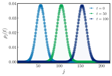
We use the exact solution of the free-fermion case to benchmark our tDMRG results. In Fig. 4, we show snapshots of typical density profiles for half filling. We find an excellent agreement between the analytical formula and the numerical simulation. Due to the relatively small variance in the Fourier space, all the one-particle states with significant probability amplitude have roughly the same velocity. As a consequence, we observe the coherent motion of the wave packet.
Oscillations in the density profile
The numerical results reveal that in the interacting case the density profile develops oscillations as soon as the counter-propagating humps start to split. This effect can be observed for the low- and high-energy regimes in Fig 5(a) and (b), respectively. To separate the alternating part from the smooth one, we evaluate the absolute value of the difference between the local charge excess in neighboring sites, defining
| (17) |
The result for is represented by the black lines in Fig. 5(b). The wave front of the alternating part moves along the smooth part of the fastest density humps, but the alternating part has a long tail that persists after the smooth part has propagated away. We stress that the alternating part does not contribute to the net charge being transported away from the region where the excitation was initially created.
We can use the effective field theory to understand how the oscillations arise only in the presence of interactions. The bosonized form of the density operator is Giamarchi (2004)
| (18) | |||||
where is a nonuniversal short-distance cutoff of the order of the lattice spacing. The second term is the staggered part that oscillates with momentum .
At low energies, we take and in Eq. (2). Setting in an infinite chain, the expectation value of the staggered part in the time-evolved state becomes
Bosonizing the fermion operators, we obtain
| (20) | |||||
where . The three-point function for the chiral vertex operators has the form
| (21) |
provided that the neutrality condition is satisfied. We then have
| (22) | |||||
From Eq. (22) we can check that there are no oscillations in the noninteracting case. Setting for , the result simplifies to
| (23) | |||||
The integral over vanishes because the integrand is an analytical function in the lower half plane. For , the integrand in Eq. (22) has branch cuts both above and below the real axis and the staggered part of the density operator acquires a nonzero expectation value. Physically, the branch points at are associated with excitations moving in opposite directions.
Momentum independence at half filling
To avoid the reflection of the wave packet at the boundaries, the time reached in the tDMRG simulations is fixed by system size and the interaction. This limitation on the maximum time may prevent distinguishing the two right-moving humps. In Fig. 6, we show the charges as a function of the LL parameter for two distinct values of . In these cases, both right and left low-energy movers can be separately resolved and we observe an excellent agreement with the nLL prediction, .
Now, for the cases in which we cannot resolve the right-moving excitations, we analyze the dynamics by assuming that the density profile consists of two symmetric counter-propagating humps with velocity and a middle one with mean velocity . We fit our results using the following equation
| (24) |
where the amplitude and the variance are obtained by fitting the left-moving wave packet. The amplitude and the variance of the high-energy wave packet are fitting parameters. In Fig. 7(a), we show combinations of three Gaussian functions that describe the time evolution of the charge wave packet. For and , the fixed parameters of the low-energy contributions are and . The free fitting parameters and depend on time and vary monotonically once the left movers can be discerned from the right-moving excitation; see Fig. 7(b).
As aforementioned, in the free-fermion case, a Gaussian wave packet of a single particle that is strongly peaked around spreads in time as . In this context, by fitting our estimates of considering the function , we obtain . Overall, we find that the combination of three Gaussian functions is consistent with our DMRG results.
Spectral decomposition of the initial excitation
In the main text, we discuss the spectral decomposition of the initial excitation for quarter filling. In addition to the signature of one-particle states, we observe the emergence of two-particle bound states, which do not exist for the half-filling case Pereira et al. (2009). Indeed, the function is characterized by a single peak in the vicinity of the high-energy particle excitations (see Fig. 8).

Wave-packet dynamics at quarter filling
In contrast to the half-filling case, where one-particle states dominate the time evolution of the Gaussian excitation, additional high-energy states play an important role at low densities. In this case, we observe that the dynamics may harbor two-particle bound states and free holes, whose fingerprint is observed in . As discussed in the main text, the minimum value of momentum for which the aforementioned composite excitation exists is
| (25) |
with . Thus, to observe the nLL prediction discussed in the main text, we must set appropriate values of and such that only single-particle excitations are created in the initial state. For instance, for and , we observe that the late-time excitation comprises a three-hump structure, as predicted by nLL. In this regime, we can describe the evolution of the initial excitation using a combination of three propagating Gaussian wave packets. In Fig. 9(a), we show snapshots of the averaged density profile for and . The decomposition of the excitation into three Gaussian functions is represented by the shaded regions in the figure. The velocities and are the obtained via Bethe ansatz. Note that the right-moving excitation is composed by one Gaussian function with a negative amplitude that follows velocity and one hump with velocity of the high-energy particle with momentum . It is worth pointing out that the negative charge carried by the low-energy right-moving hump is consistent with the nLL description, . In general, we found a good agreement between the combination of three Gaussian functions and the tDMRG results as long as we do not have composite excitations in the dynamics.
Finally, let us briefly discuss a case where we see signatures of the bound states, but we can still discern the left- and right-propagating excitations; see Fig. 9(b). Depending on , the left-moving wave packet is not only composed by low-energy movers, but a combination of excitations with velocity close to . Indeed, the tail of the left wave packet in Fig. 9(b) suggests the existence of holes propagating with velocity close to the Fermi one.