Benchmarking Deep Jansen-Rit Parameter Inference: An in Silico Study

Abstract

The study of effective connectivity (EC) is essential in understanding how the brain integrates and responds to various sensory inputs. Model-driven estimation of EC is a powerful approach that requires estimating global and local parameters of a generative model of neural activity. Insights gathered through this process can be used in various applications, such as studying neurodevelopmental disorders. However, accurately determining EC through generative models remains a significant challenge due to the complexity of brain dynamics and the inherent noise in neural recordings, e.g., in electroencephalography (EEG). Current model-driven methods to study EC are computationally complex and cannot scale to all brain regions as required by whole-brain analyses. To facilitate EC assessment, an inference algorithm must exhibit reliable prediction of parameters in the presence of noise. Further, the relationship between the model parameters and the neural recordings must be learnable. To progress toward these objectives, we benchmarked the performance of a Bi-LSTM model for parameter inference from the Jansen-Rit neural mass model (JR-NMM) simulated EEG under various noise conditions. Additionally, our study explores how the JR-NMM reacts to changes in key biological parameters (i.e., sensitivity analysis) like synaptic gains and time constants, a crucial step in understanding the connection between neural mechanisms and observed brain activity. Our results indicate that we can predict the local JR-NMM parameters from EEG, supporting the feasibility of our deep-learning-based inference approach. In future work, we plan to extend this framework to estimate local and global parameters from real EEG in clinically relevant applications.

1 Introduction

For about half a century, neural mass models (NMM) have been used to depict the collective behavior of extensive groups of neurons [47, 46, 26, 6]. These models have proven effective in investigating neural activity captured by neuroimaging modalities such as electroencephalography/magnetoencephalography (EEG/MEG) [40, 7] and functional magnetic resonance imaging (fMRI) [24]. Besides helping in understanding fundamental properties of neural dynamics, these models were used in multiple applications, including the study of transcranial magnetic stimulation effect on neural activity [4], altered states of consciousness [23], brain dynamics in epilepsy [45] and Alzheimer’s disease [41], to name only a few. They also have become a fundamental component of whole-brain simulation frameworks [31] as proposed by The Virtual Brain (TVB) [38] and neurolib [3].

Variations in NMM parameters can explain observed changes in neuroimaging data, particularly under pathological conditions [30, 44]. By adjusting parameters, NMMs can reproduce various processes and exhibit different dynamical behaviors observed experimentally [7, 46, 39]. However, the accurate estimation of NMM parameters is challenging due to the complexity and noisiness of neural activity, compounded by the under-defined nature of the NMM parameter inference problem. Traditional methods (e.g., gradient-based optimization [27], dynamic causal modeling (DCM) [7], and Bayesian techniques [15, 5]) are computationally demanding. Further, they are generally inadequate for handling large datasets or real-time analysis due to their tendency to converge towards local minima and their dependency on strong prior assumptions.

This paper explores the application of deep learning to estimate local parameters modeling dynamics in the Jansen-Rit Neural Mass Model (JR-NMM) within specific brain regions. In contrast, global parameters involve the coupling of neural masses across different regions. By assessing deep learning’s capacity to infer local parameters, this in silico benchmarking study sets the groundwork for future studies on global parameters and inference on real EEG. Here, we propose a novel strategy that includes 1) a detailed examination of how local JR-NMM parameters affect event-related potentials (i.e., sensitivity study) and 2) a parameter estimation technique using a bidirectional long short-term memory (Bi-LSTM) model.

2 Related Work

The estimation of NMM parameters can be framed in terms of conditional probabilities. To estimate conditional distribution over some parameters $\theta$, observational data $x$ are employed to compute the posterior distribution $p(\theta|x)$. Certain parameters within $\theta$ can be closely related, leading to structured outcomes where only a few configurations of these parameters are likely. This often happens when the parameters interact in a way that allows one parameter to be adjusted up or down while another is changed in the opposite direction, but without affecting the overall results of the model. This kind of situation is referred to as a “partially identified model" in statistics and econometrics [18], and it can make the model difficult to handle or “ill-posed."

Gelman et al. utilized a hierarchical Bayesian model [10] to address the challenges of ill-posed estimation problems. In their approach, the parameters for individual observations, $\theta_{i}$, are segregated into sample-specific (local) parameters, $\alpha_{i}$, and shared (global) parameters, $\beta$. Consequently, the posterior distribution for a collection of $N$ observations, $X=\{x_{1},\dots,x_{N}\}$, is formulated as: $p(\alpha_{1},\dots,\alpha_{N},\beta|X)\propto p(\beta)\prod_{i=1}^{N}p(x_{i}|\alpha_{i},\beta)p(\alpha_{i}|\beta)$. Hierarchical models capitalize on statistical strengths across observations to refine the posterior distributions and enhance the reliability of parameter estimates. They are applicable in various domains, including topic modeling [2], matrix factorization [36], Bayesian nonparametric methods [42], and population genetics [1]. But, they can be computationally very intensive, especially with a large number of parameters.

Traditional Markov Chain Monte Carlo (MCMC) methods are often used for Bayesian inference due to their robustness in sampling from complex posterior distributions. However, these methods prove unsuitable when the likelihood function $p(x_{i}|\alpha_{i},\beta)$ is implicit and intractable [34]. This limitation has prompted the adoption of likelihood-free inference (LFI) techniques. Recent developments in LFI have introduced algorithms that learn different components of Bayesian inference, such as the likelihood function, the likelihood-to-evidence ratio, or the posterior itself [29, 16, 19, 9, 34]. These methods are notably effective in hierarchical model settings. However, LFI methods typically have a limited scope regarding the number of parameters they can estimate accurately. This limitation arises because LFI algorithms often require many simulations to approximate the target distributions accurately, which becomes prohibitively computationally expensive as the number of parameters increases. Additionally, the complexity of the underlying models can further constrain the efficiency and scalability of LFI techniques.

Further challenges are encountered in neuroscience, specifically with approaches like DCM for EEG/fMRI [7, 28, 32, 35], which, despite being effective for inferring global parameters, falls short when we introduce more complex networks, such as those describing specific synaptic or neural population properties within a more extensive network [25]. DCM is often restricted to a limited number of brain regions rather than encompassing the entire brain [35]. TVB, a simulation-based framework, has significantly advanced the precision of simulation for biophysical models in neuroscience, aiding in estimating brain properties [37]. However, TVB does not support parameter estimation due to the larger number of parameters associated with whole-brain simulations complicating the accurate fitting of models to empirical data [33]. Furthermore, estimating biophysical parameters that are not directly observable through imaging techniques presents significant challenges, typically requiring indirect inference methods that introduce uncertainties [22]. Recently, deep learning methods, which typically require large datasets to achieve high accuracy and generalizability, have been adapted to address the limitations of dynamical models, especially where data is scarce, noisy, or costly to acquire [11]. A new approach for parameter estimation in connectome-based NMM utilizing deep learning has recently been introduced. This method has shown enhanced robustness and improved accuracy in the recovery of parameters, as evidenced by tests on both synthetic and real human connectome fMRI data [17]. Here, we propose to adopt a similar deep-learning approach for the model-driven analysis of EC in EEG using JR-NMM.

3 Methods

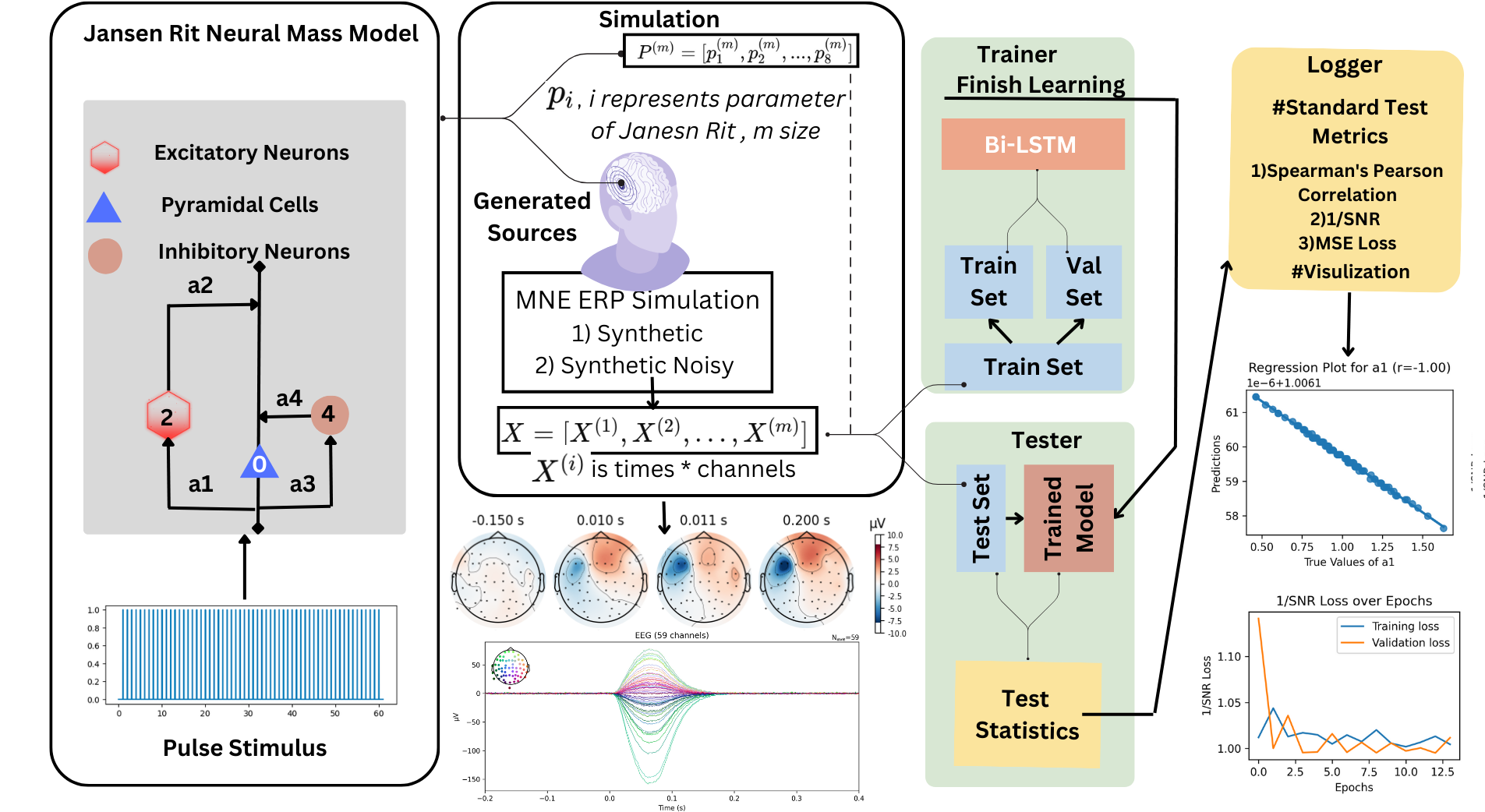
Figure 1: Our approach employs the JR-NMM to simulate Event-Related Potentials (ERP), integrating a Bi-LSTM network for robust parameter estimation. This figure illustrates the workflow from model simulation to parameter inference, culminating in evaluating performance metrics.

Jansen-Rit Neural Mass Model:

The Jansen-Rit model [21], building upon the foundational work by Lopes da Silva et al. [26], is designed to simulate interactions within cortical areas through networks of excitatory and inhibitory neurons. These cortical areas are conceptualized as ensembles of macro-columns, where each macro-column contains excitatory pyramidal cells receiving both local and distant excitatory and inhibitory feedback. This complex interaction underpins the generation of cortical oscillations. Understanding this generative process is essential for elucidating various brain functions and pathologies. The model receives external inputs (e.g., from other cortical or subcortical regions, or the peripheral nervous system), specifically $I_{p}$ for pyramidal neurons and $I_{i}$ for inhibitory neurons. Several key transformations characterize the dynamics of the JR-NMM [7]:

1. Synaptic input to membrane potential transformation: The average density of presynaptic action potentials ($b(t)$), including the external inputs $I_{p}(t)$ and $I_{i}(t)$, is converted into the contribution $y_{i}(t)$ of the presynaptic population $i$ to the average postsynaptic membrane potential via convolution (denoted by $\otimes$) with the impulse response function $c(t)$ capturing the synaptic kinetics. That is, $y(t)=c(t)\otimes b(t)$, where the impulse response $c(t)$ is described by:

   $$c(t)=\begin{cases}\frac{H}{\tau}\exp\left(-\frac{t}{\tau}\right)&\text{if }t\geq 0\\ 0&\text{if }t<0\end{cases}$$ (1)

   The parameters $H$ and $\tau$ modulate, respectively, the amplitude and decay rate of the synaptic response to presynaptic action potentials.

2. Membrane potential to axonal output transformation: The sigmoid function $S(v)$ translates the mean membrane potential $v$ of a specific population into its mean firing rate. It is expressed as:

   $$S(v)=S_{max}.\frac{1}{1+e^{-r(v-v_{0})}}$$ (2)

   The parameters $v_{0}$ and $r$ regulate the midpoint and steepness of the sigmoidal curve, whereas $S_{max}$ captures the maximal firing rate for the population. As $v$ increases, $S(v)$ gradually rises from 0 to $S_{max}$, capturing the activation level of the neuron population. We used $v_{0}=6$, $r=0.56$ and $S_{max}$ = 5 spikes per second.

The following state-space equations describes the dynamics of JR-NMM:

$$\dot{y}_{0} =y_{1},$$

$$\dot{y}_{1} =A_{e}b_{e}S(I_{p}+a_{2}y_{2}-a_{4}y_{4})-2b_{e}y_{1}-b_{e}^{2}y_{0},$$

$$\dot{y}_{2} =y_{3},$$

$$\dot{y}_{3} =A_{e}b_{e}S(a_{1}y_{0})-2b_{e}y_{3}-b_{e}^{2}y_{2},$$ (3)

$$\dot{y}_{4} =y_{5},$$

$$\dot{y}_{5} =A_{i}b_{i}S(I_{i}+a_{3}y_{0})-2b_{i}y_{5}-b_{i}^{2}y_{4}$$

Indices 0, 2, and 4 represent the pyramidal, excitatory neuron, and inhibitory neuron populations, respectively, as illustrated in Figure 1. All parameters used in the equations are defined in Table 1, in supporting information.

The output signal $y(t)=a_{2}y_{2}-a_{4}y_{4}$ represents the difference between the pyramidal’s excitatory and inhibitory postsynaptic potentials. This value is a proxy for EEG sources because EEG is thought to reflect mainly the postsynaptic potentials in the apical dendrites of pyramidal cells. The use of JR-NMM in our simulation is shown in Algorithm 1. The low and high parameter values used in the equations above are shown in Table 1 (in supporting information).

Jansen-Rit Simulation:

Algorithm 1 Simulation of Sources from Jansen-Rit

1:procedure Generate_Stimulus($dt,T_{\text{tot}},\text{events},\text{pulse\_width\_fraction}$)

2:     $t\leftarrow[0,dt,2dt,\ldots,T_{\text{tot}})$

3:     $I\leftarrow[0,0,\ldots,0]$ $\triangleright$ Length of $t$ (i.e., L elements)

4:     $n_{\text{samp\_stim}}\leftarrow\text{round}(1/dt\cdot\text{pulse\_width\_fraction})$

5:     for $\text{ind}\in\text{events}$ do

6:         $I[\text{ind}:\text{ind}+n_{\text{samp\_stim}}]\leftarrow 1$

7:     end for

8:     $I_{p}\leftarrow 60\cdot I$ $\triangleright$ Modified input for pyramidal

9:     $I_{i}\leftarrow 60\cdot r\cdot I$ $\triangleright$ Modified input for inhibitory, using r = 0.56, constants taken from [7]

10:     return $I_{p},I_{i},t$

11:end procedure

12:procedure JR_NMM_Simulation($dt$, $L$, $I_{p}$, $p$, $params$)

13:     Initialize state variables $y\leftarrow\text{zeros}(6,L)$ $\triangleright$ Initialize state array to store results

14:     $A_{e},A_{i},b_{e},b_{i},a_{1},a_{2},a_{3},a_{4}\leftarrow params$ $\triangleright$ Extract parameters from input

15:     for $t\leftarrow 1$ to $L$ do $\triangleright$ Update dynamics with Euler’s method

16:         $\dot{y}_{0}\leftarrow y_{1}$ $\triangleright$ Derivative of $y_{0}$

17:         $\dot{y}_{1}\leftarrow A_{e}b_{e}S(I_{i}+a_{2}y_{2}-a_{4}y_{4})-2b_{e}y_{1}-b_{e}^{2}y_{0}$ $\triangleright$ Derivative of $y_{1}$

18:         $\dot{y}_{2}\leftarrow y_{3}$ $\triangleright$ Derivative of $y_{2}$

19:         $\dot{y}_{3}\leftarrow A_{e}b_{e}S(a_{1}y_{0})-2b_{e}y_{3}-b_{e}^{2}y_{2}$ $\triangleright$ Derivative of $y_{3}$

20:         $\dot{y}_{4}\leftarrow y_{5}$ $\triangleright$ Derivative of $y_{4}$

21:         $\dot{y}_{5}\leftarrow A_{i}b_{i}S(I_{p}+a_{3}y_{0})-2b_{i}y_{5}-b_{i}^{2}y_{4}$ $\triangleright$ Derivative of $y_{5}$

22:         $y[:,t]\leftarrow[\dot{y}_{0},\dot{y}_{1},\dot{y}_{2},\dot{y}_{3},\dot{y}_{4},\dot{y}_{5}]$ $\triangleright$ Store current state in the array

23:     end for

24:     return $y$ $\triangleright$ Return the array containing the state variables

25:end procedure

Algorithm 2 Generate Evoked Responses from EEG Simulation and Parameter Analysis

1:procedure GENERATE_EVOKED_FROM_JR($a_{2}$, $a_{4}$, $\alpha$, $\Sigma$)

2:     $\mathbf{F}\leftarrow$ Compute the lead field $\triangleright$ (more details in supporting subsection Generate Evoked Potentials from JR-NMM)

3:     $y\leftarrow$ JR_NMM_Simulation(…)

4:     $S(t)\leftarrow a_{2}y_{2}(t)-a_{4}y_{4}(t)$

5:     $\text{EEG}(t)\leftarrow\mathbf{F}\cdot S(t)$

6:     if $\alpha>0$ then

7:         $\text{EEG}_{\text{noisy}}(t)\leftarrow\text{EEG}(t)+\alpha\cdot\mathcal{N}(t;0,\Sigma)$

8:     end if

9:     Compute SNR: $\text{SNR}_{\text{dB}}=10\log_{10}\left(\frac{\text{mean}(\text{EEG}(t)^{2})}{\text{mean}((\text{EEG}_{\text{noisy}}(t)-\text{EEG}(t))^{2})}\right)$

10:     Extract epochs and compute the evoked response

11:     return Evoked responses and SNR

12:end procedure

13:procedure Simulate_For_Parameter($param\_key$, $param\_range$, $params$)

14:     $params[param\_key]\leftarrow$ Sample parameter values within $param\_range$

15:     $I_{p},I_{i}\leftarrow$ GENERATE_STIMULUS(..)

16:     for each sampled parameter value do

17:         Run JR_NMM_Simulation using $params$, $I_{p}$, and $I_{i}$

18:         Generate responses using GENERATE_EVOKED_FROM_JR

19:     end for

20:end procedure

The simulation module simulates neural dynamics with or without noise (see Figure 7 in appendix). It relies on MNE-Python [13] to simulate the EEG from JR-NMM sources placed in specific regions of the Destrieux atlas [8]. The detailed simulation process is explained in Algorithm 1 and Algorithm 2. More technical details of these procedures are available in supporting information (subsection 7.1). We use this simulated dataset for training, validation, and testing. The dependent variables (i.e., the JR-NMM local parameters) in our regression analysis are represented as $P^{(m)}=[p_{1}^{(m)},p_{2}^{(m)},\ldots,p_{8}^{(m)}]$, where m = 1000. We sampled parameter values from normal distributions, setting the mean to the midpoint of the parameter ranges defined in Table 1 and the standard deviation to 1/4 of this range. This operation ensured that about 95% of the samples fell within the range. Values outside this range were truncated, resulting in truncated normal distributions. Our experiments were conducted on a machine with an Apple M1 Pro CPU and 32 GB of RAM. Every event-related potential (ERP) simulation took approximately 1 second, in average. ERPs are obtained by averaging the EEG signal over multiple trials to reduce noise and enhance the signal related to the stimulus, as normally done with EEG recorded using event-related paradigms. We averaged 60 trials for the ERP, consistent with standard experimental practices.

Sensitivity Analysis:

Before proceeding with the inference, we performed a sensitivity analysis to evaluate how changes in model parameters influenced the corresponding ERPs. This analysis was necessary for understanding whether the ERPs (i.e., the experimental observations) were sensitive to changes in parameter values (i.e., the latent variables we aim to estimate) and, therefore, determine if the value for the latent variables can reliably be predicted from the ERPs.

To assess how the shape of the ERP changes as a function of JR-NMM parameter values, for each parameter, we conducted 200 simulations varying this parameter using values evenly distributed within the ranges in Table 1. We did not introduce noise in these simulations. When analyzing the effect of one parameter, the others were held constant at the middle value of their ranges. This allowed us to isolate the impact of individual parameters on the model’s output.

To understand how parameter variations influence ERPs, we computed the average ERP across all simulations ($S_{\text{mean}}$) and compared the ERP for distinct parameter values ($S_{\text{param}}$) against this overall average. We calculated the squared relative error $\log_{10}\left(\frac{S_{\text{param}}-S_{\text{mean}}}{S_{\text{mean}}}\right)^{2}$ and the squared absolute error $(S_{\text{param}}-S_{\text{mean}})^{2}$. The relative error is computed on a logarithm base-10 scale to manage the wide range of values and enhance interpretability. Heatmaps were created to illustrate how the ERP and the relative and absolute errors vary as a function of the JR-NMM parameters.

Estimation using Bi-LSTM:

Long Short-Term Memory (LSTM) [20] networks are a type of recurrent neural network capable of learning long-term dependencies, especially useful for sequence prediction problems. LSTM networks introduce a memory cell that can maintain information over long sequences, addressing the vanishing gradient problem common in traditional RNNs. The hidden states in an LSTM network, denoted as ${h}_{t}$, capture the relevant information from the input sequence up to time $t$. We employed a bidirectional LSTM [14], enabling the network to capture dependencies from the input sequence’s past (backward) and future (forward) directions. This is crucial because the brain’s response patterns, as reflected in EEG signals, are influenced by temporal dynamics that unfold in both directions. This is represented mathematically as $\text{Bi-LSTM}(\mathbf{x}_{t})=\overrightarrow{\text{LSTM}}(\mathbf{x}_{t},\overrightarrow{h}_{t-1})\oplus\overleftarrow{\text{LSTM}}(\mathbf{x}_{t},\overleftarrow{h}_{t+1})$ where $\oplus$ denotes the concatenation of the forward and backward LSTM outputs. These model outputs include hidden states $\overrightarrow{h}_{t}$ and $\overleftarrow{h}_{t}$, and the input feature $\mathbf{x}_{t}$, where the index $t$ indicates the corresponding time sample. A dropout rate of 0.1 is applied to the Bi-LSTM layer to prevent overfitting. This dropout randomly sets a fraction of the input (10% in our case) to zero during training. Flattening from a 64-unit vector to an 8-unit vector is accomplished through a dense layer, consolidating the entire sequence into a single output vector $p$. This vector $p$ is computed as $p=\mathbf{W}\mathbf{h}_{t}+\mathbf{b}$. Here, $W$ is the weight matrix of the dense layer, initialized using Glorot Uniform [12] with a seed of 4287, and $b$ is the bias vector, set to 0.001. The kernel and bias initializer constant helps prevent the gradient from exploding or vanishing. A linear activation ensures that the final output $p$ effectively captures the condensed information from the LSTM features across the temporal dimension.

The dataset was divided into training (80%), validation (10%), and testing (10%) sets to ensure unbiased and generalizable evaluation. The Adam optimizer was selected to handle sparse gradients in noisy environments effectively. A custom loss function was implemented based on the inverse of the signal-to-noise ratio (1/SNR; SNR as defined in Algorithm 2). We used an early stopping mechanism that terminates training if the validation loss is not decreased after ten epochs to conserve computational resources and prevent overfitting. We trained our model for 150 epochs with a batch size of 32. The simulation and inference code developed in our experiments is accessible at the GitHub repository (https://github.com/lina-usc/Jansen-Rit-Model-Benchmarking-Deep-Learning).

4 Results

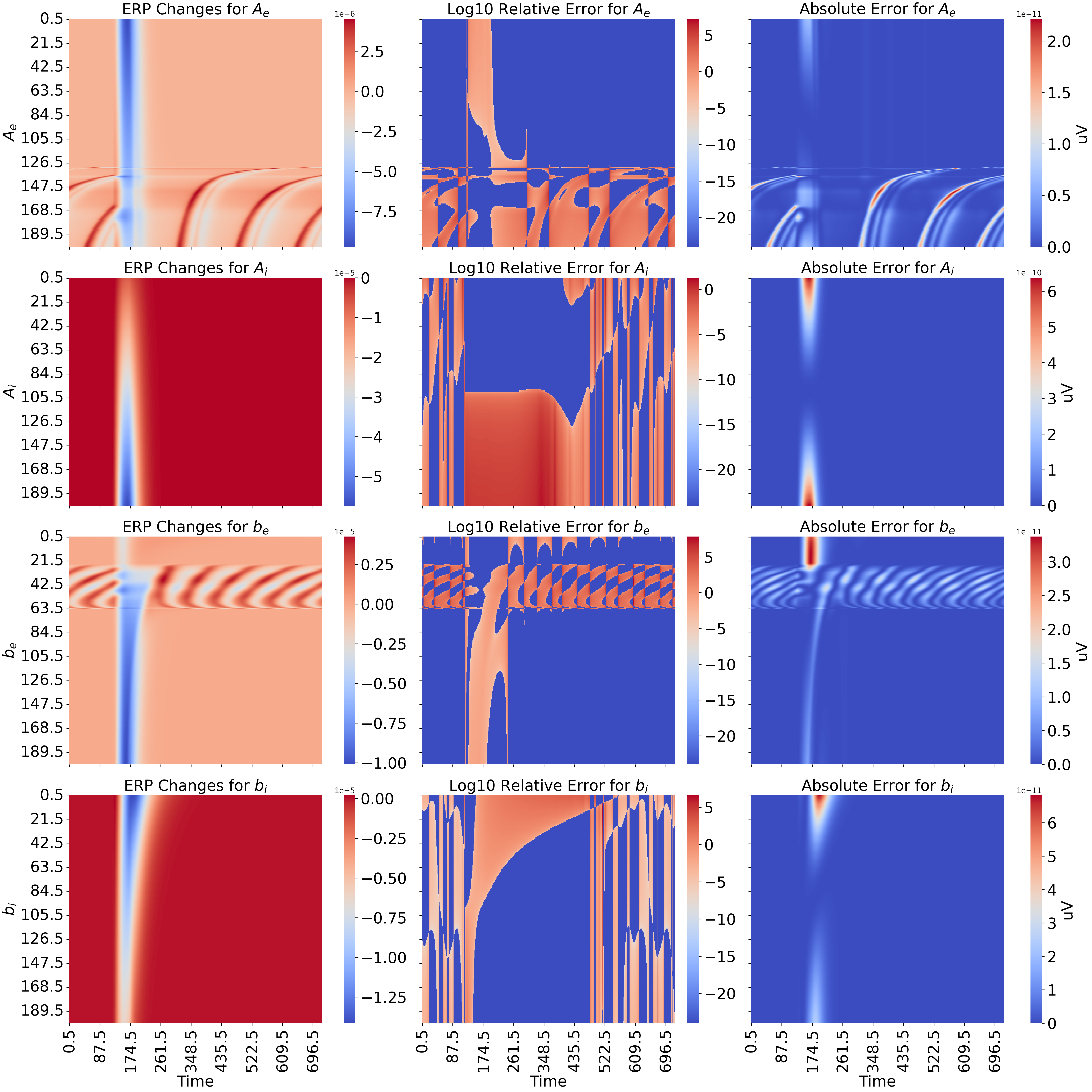
Figure 2: Sensitivity plot for parameters $A_{e}$, $A_{i}$, $b_{e}$, and $b_{i}$. The leftmost column depicts the ERP amplitude (color-coded; in V) as a function of time (x-axis) and parameter values (y-axis). The middle and rightmost columns show similar information but for the relative error (on a logarithmic scale) and the absolute error, respectively. A separate figure in the appendix (Figure 6) presents sensitivity plots for parameters $a_{1}$ to $a_{4}$.

Sensitivity Analysis:

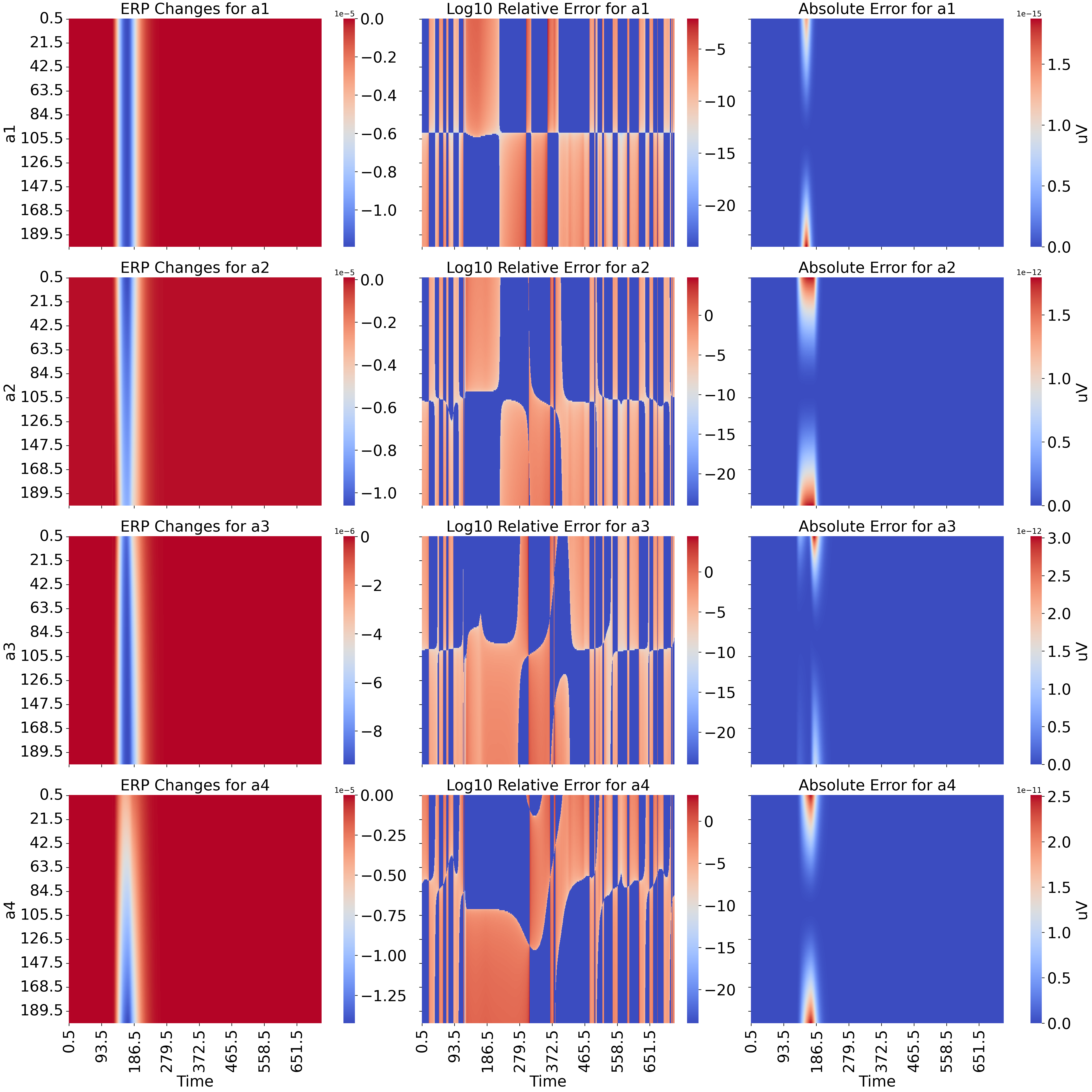
Figure 6: Sensitivity analysis for parameters $a1$, $a2$, $a3$, and $a4$. The leftmost column depicts the ERP amplitude (color-coded; in V) as a function of time (x-axis) and parameter values (y-axis). The middle and rightmost columns show similar information but for the relative error (on a logarithmic scale) and the absolute error, respectively.

The results of our sensitivity analysis are summarized in Figure 2 and Figure 6, which consist of three columns for each parameter: ERP, relative error, and absolute error. The analysis reveals that certain parameters substantially impact the EEG output. The ERP (first column) exhibits noticeable variations as the values of $A_{e}$ and $b_{e}$ change, with what appears to be an oscillatory regime around $[7.3,9.7]$ for $A_{e}$ and $[24.23,51.11]$ for $b_{e}$. The existence of these bands indicates bifurcations around which small variations in parameter values can lead to large changes in EEG behavior. These variations are further supported by deviations in the absolute error plots (third column), indicating that these parameters are likely to have enough influence on the ERP to be estimable from EEG observations. The relatively uniform changes in ERP for $A_{i}$, $b_{i}$, and $a_{4}$ indicate a more consistent sensitivity across the parameter range, compared to $A_{e}$ and $b_{e}$, with no apparent bifurcation. This suggests these parameters will have a more predictable impact on ERP under noisy conditions. In contrast, several parameters, including $a_{1}$, $a_{2}$, and $a_{3}$, show minimal impact on the ERP. The ERP patterns for these parameters remain largely unchanged across different values, and the error plots (both relative and absolute) exhibit minimal deviations.

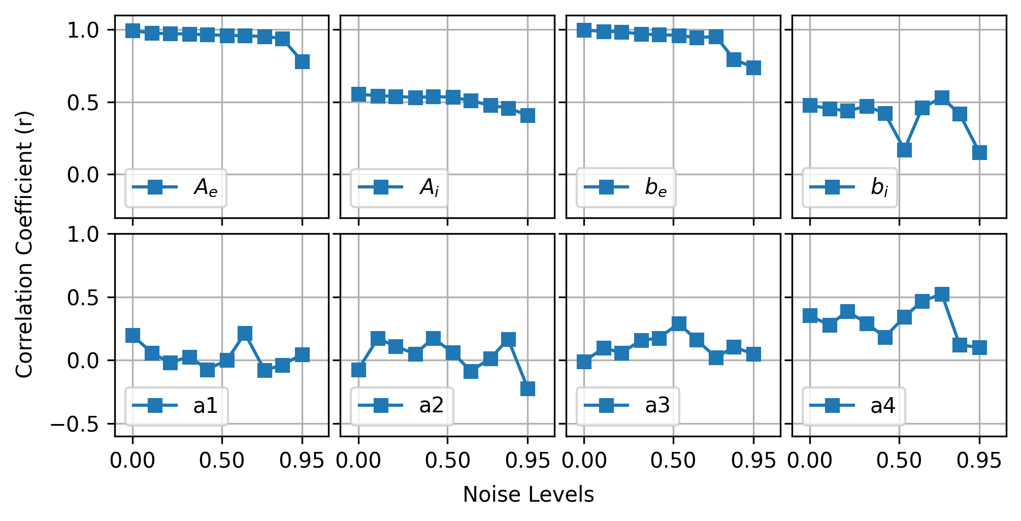
Figure 3: Impact of increasing noise levels on correlation coefficients between parameter values used for simulation and values predicted using Bi-LSTM.

Deep Learning Analysis:

In our study, we analyzed the impact of increasing noise levels (for $\alpha\in[0,0.95]$ on the correlation coefficients of eight JR-NMM parameters ($A_{e}$, $B_{i}$, $b_{e}$, $b_{i}$, $a_{1}$, $a_{2}$, $a_{3}$, and $a_{4}$) using predictions from a Bi-LSTM network (Figure 3). Both $A_{e}$ and $b_{e}$ started with almost perfect prediction, but their correlation gradually declined as noise levels increased, as would generally be expected. $A_{e}$ showed a consistent decrease from 0.995 to 0.782, highlighting its robustness yet susceptibility to higher noise levels. The initial correlation of $A_{i}$ was 0.56, which decreased to 0.4 under noisy conditions. $a_{4}$ and $b_{i}$ showed somewhat similar trends and unreliable patterns, but starting with correlations for $b_{i}$ around 0.5-0.55 and $a_{4}$ around 0.37-0.55 in noise-free condition, as opposed to the $\approx 1.0$ for $A_{e}$ and $b_{e}$. The parameters $a_{1}$, $a_{2}$, and $a_{3}$ showed an inconsistent behavior under noise.

5 Discussions

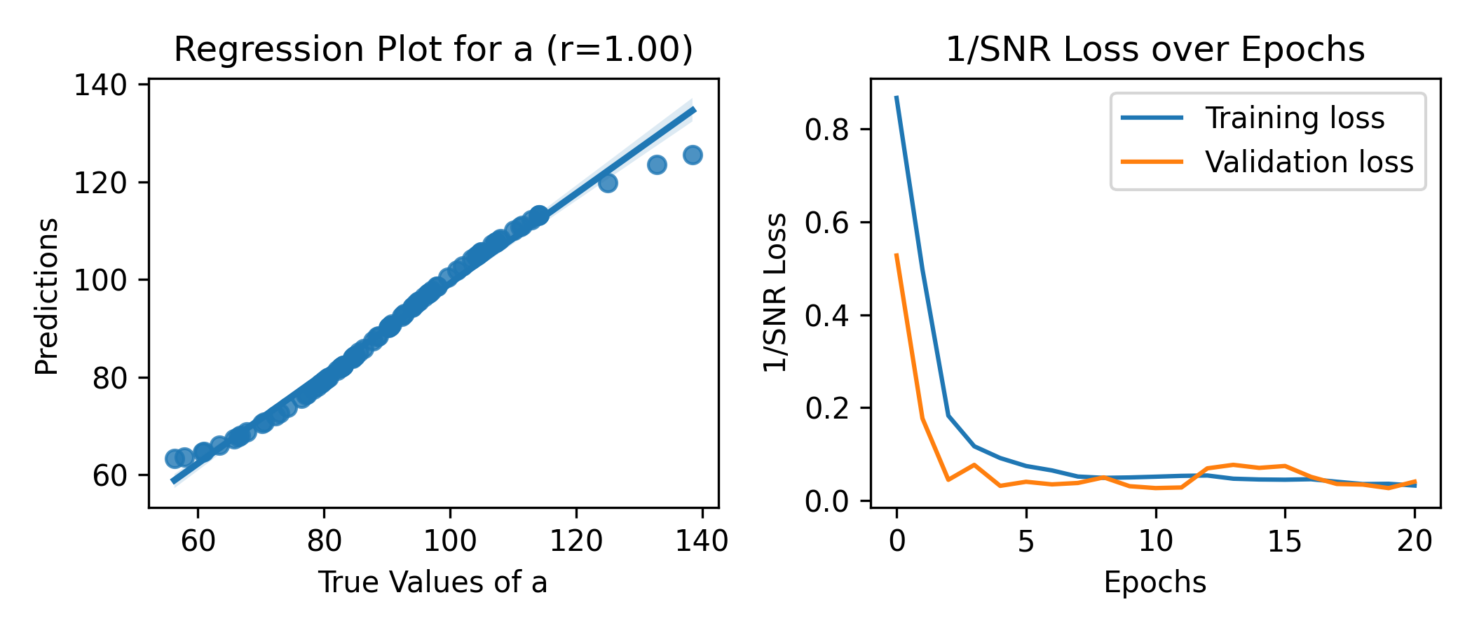
(a) a

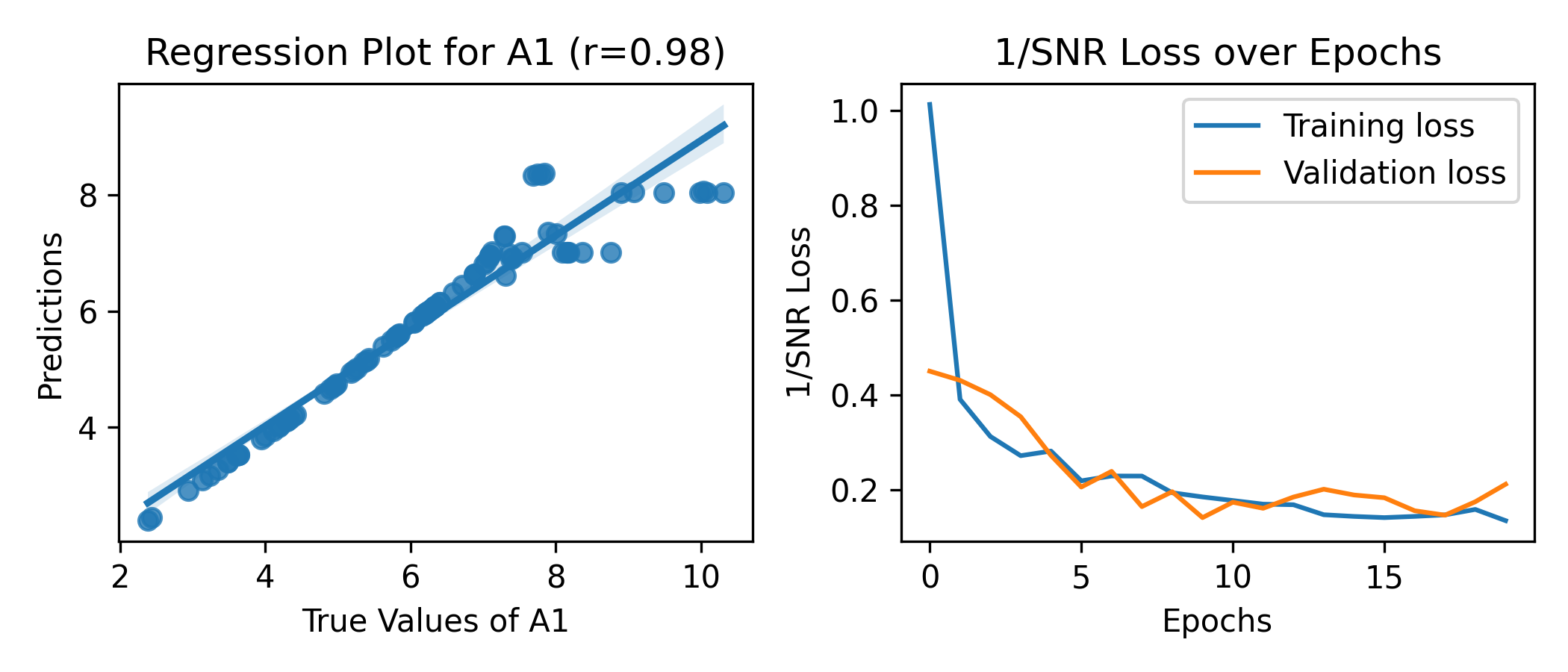
(b) A1

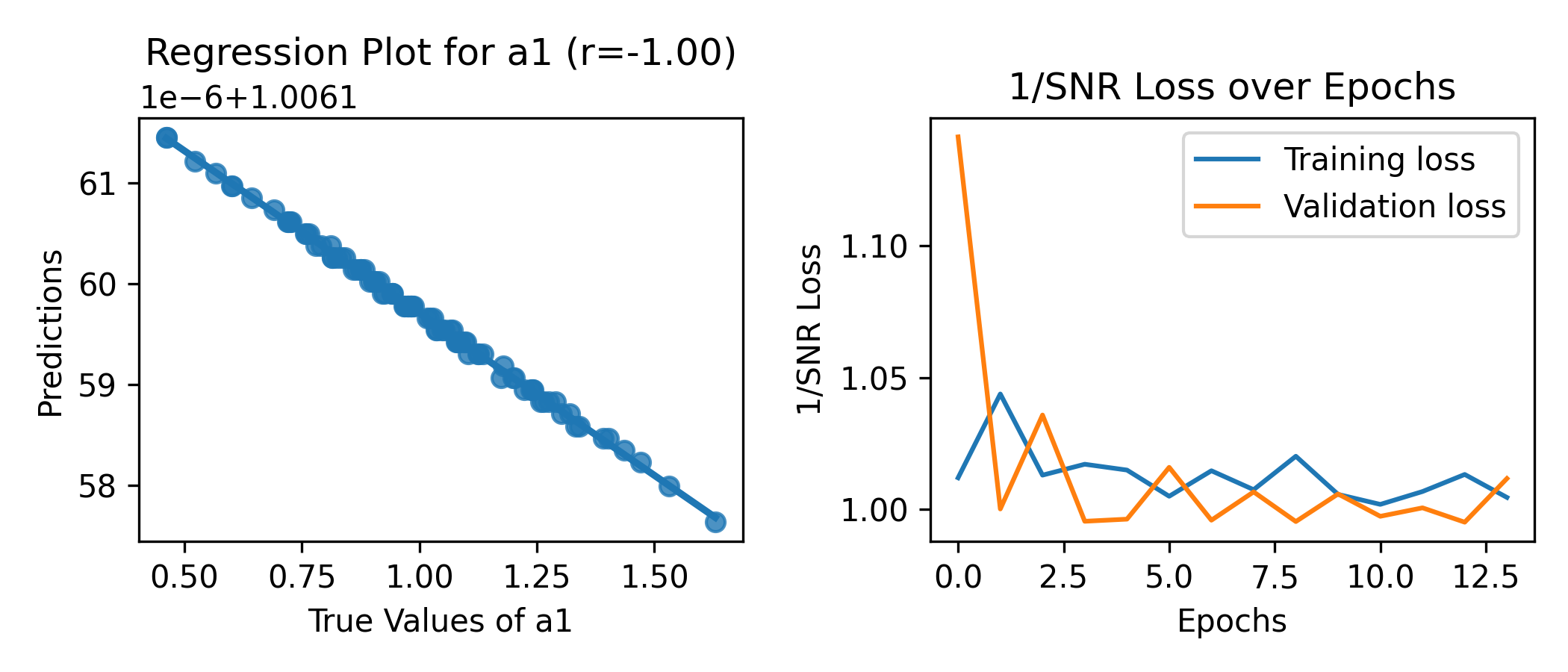
(c) a1

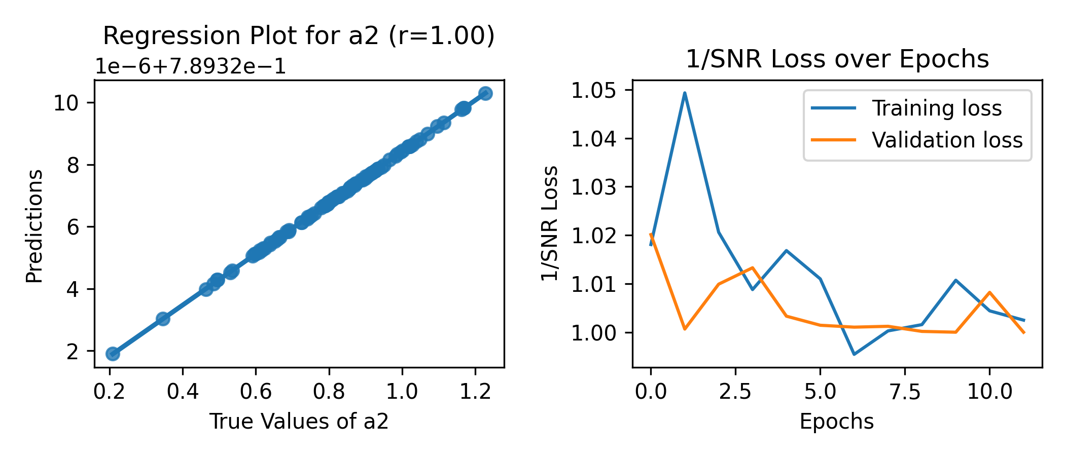
(d) a2

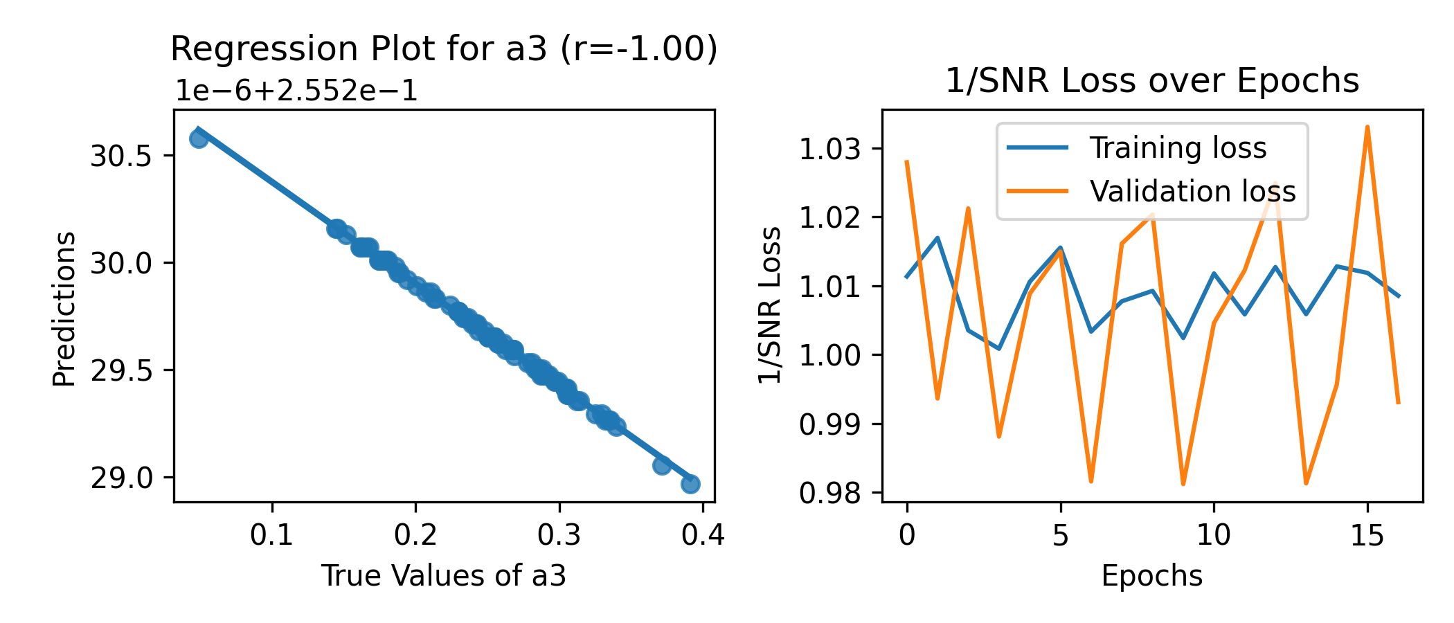
(e) a3

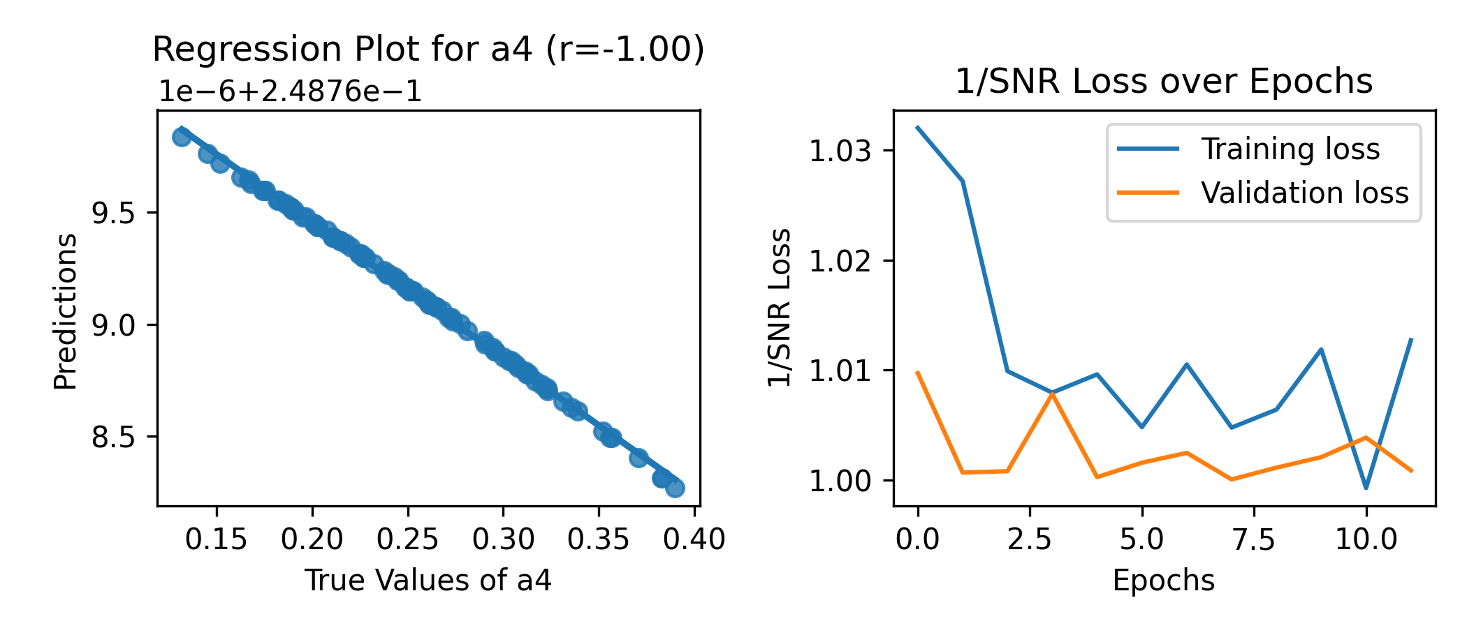
(f) a4

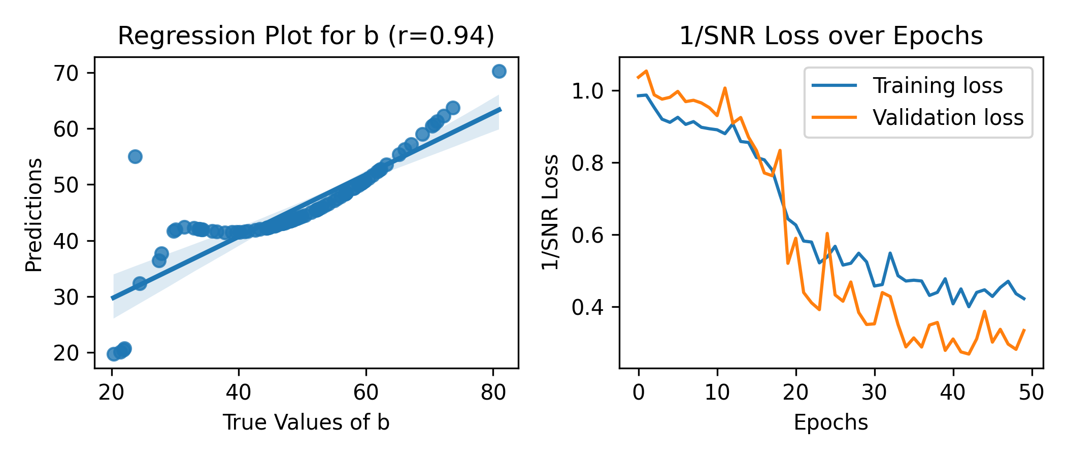
(g) b

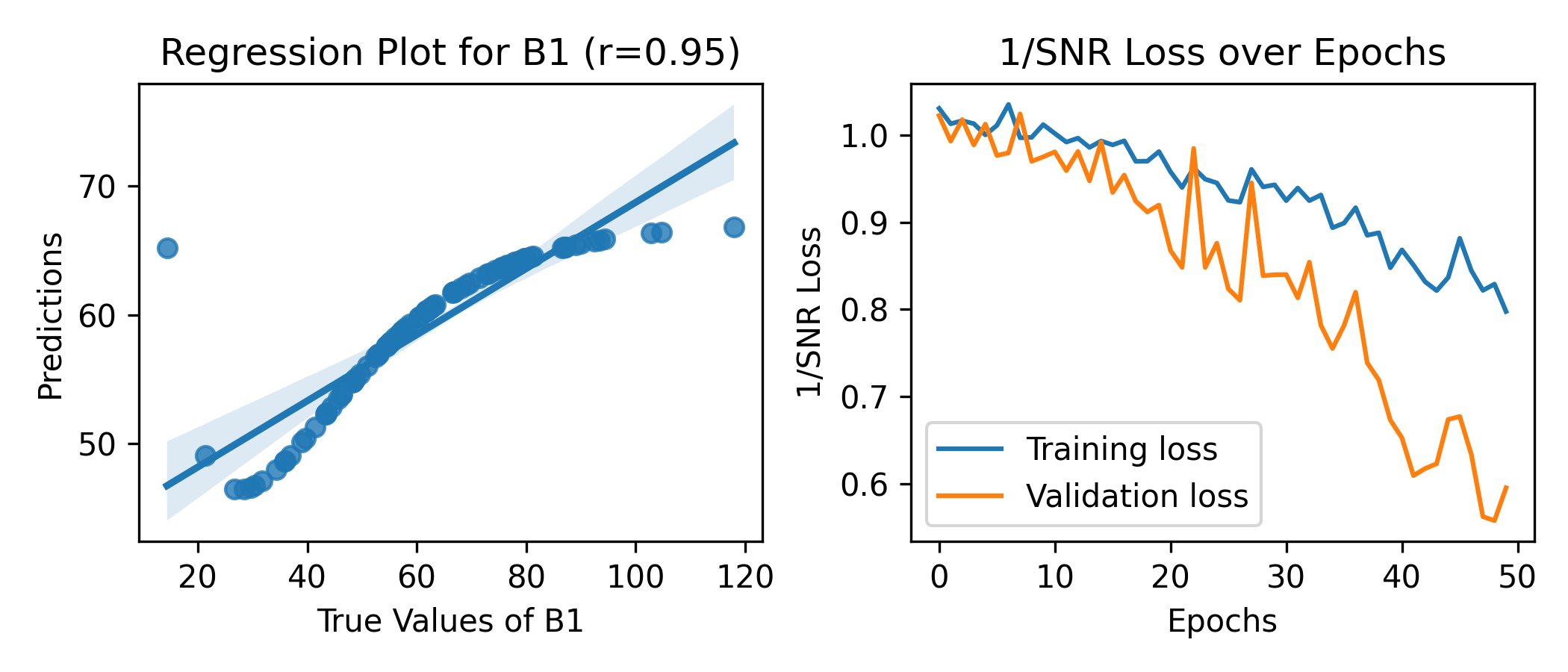
(h) B1

Figure 5: Results from a bi-LSTM model estimating one parameter at a time. Simulations were conducted by keeping other parameters constant at their mean values and varying only the parameter to be predicted.

Our study addresses the challenge of estimating the local parameters of these NMMs from EEG, which is also important for doing EC analysis. The experiments on the simulated EEG data confirm that some of the local parameters of NMMs can be estimated with sufficient confidence. Our sensitivity analysis indicates that parameters $A_{e}$ and $b_{e}$ significantly impact EEG, while other parameters like $a_{1}$−$a_{4}$ exhibit minimal influence. This examination shows that the associations between parameters and observed ERPs are learnable. We performed inference of JR-NMM parameters using EEG to examine the utility of Bi-LSTM on the correctness of parameter estimation. Initially, we simulated ERPs by changing each parameter separately while keeping the rest at their mean values and estimating only one parameter at a time. Interestingly, the Bi-LSTM model showed a correlation coefficient of 1.0 for most of these parameters (see supplementary material Figure 5). However, when we increased the complexity of the inference by simultaneously estimating all parameters together, our analysis showed that some parameters, specifically synaptic gains ($A_{e}$, $A_{i}$) and the time constant $b_{e}$, significantly impact the ERPs. This influence was also notable under varying noise conditions. Our experiments, involving noise-free and noisy EEG simulations, demonstrated that our deep learning approach using a Bi-LSTM network can estimate these parameters, reflecting their potential for accurate and reliable inference.

By developing this approach, we aim to improve the prediction of JR-NMM parameters. We will extend this study further to estimate global parameters in simulations involving sources placed in multiple brain regions to demonstrate the full potential of this approach. However, we hope that the power of deep learning combined with the possibility of simulating as large of a training set as necessary may offer a more scalable and efficient approach to parameter estimation in complex NMMs. Future work should extend this approach to observed EEG data to validate the findings from synthetic data. Understanding the interplay between different parameters and their collective impact (i.e., multivariate analyses) on EEG output will also be crucial for developing more comprehensive and accurate neural models.

Limitations:

Despite the promising results, our study has several limitations. This analysis was conducted on simulated EEG data, which may not fully capture the complexities and variabilities of real EEG signals. Validation with observed EEG data is necessary to confirm the applicability of our findings. While we analyzed the impact of noise on parameter estimation, real EEG data may contain more complex noise patterns that were not fully accounted for in our simulations. Furthermore, as the noise level surpassed the critical threshold of 0.95 in our simulations, the model consistently predicted identical parameter values, leading to a NaN value for the correlation coefficient. The reason for this behavior is unknown and require investigation. While Bi-LSTM serves as a viable baseline, its capacity to generalize across diverse datasets, handle noise levels beyond a factor of 1 (i.e., the noise equal to the level observed in real EEG), and adapt to various experimental conditions requires comprehensive evaluation. Our study focused on inferring local parameters within a single brain region. In contrast, the more complex problem of predicting global parameters across multiple brain regions, i.e., EC, was not explored. Understanding these interdependencies is crucial for extending the study to examine EC, which remains beyond the scope of this study.

6 Conclusion

Our study reports on a sensitivity analysis demonstrating which parameters in the JR model are likely to be learnable from ERPs. The results show varying degrees of sensitivity to noise across different parameters. Insensitive parameters (i.e., the $a_{i}$ parameters in general) are unlikely to have a significant role in the dynamics of the JR-NMM model and to be predicted with accuracy from EEG. Further, we used deep learning models trained on simulated evoked data to analyze the performance of JR-NMM parameter inference. By identifying key parameters and understanding their sensitivity to noise, we can refine our models to capture the underlying neural processes better, leading to more accurate interpretations of EEG. The insights gained from this research will support a better understanding of the potential and limitations of the JR model for parameter inference from EEG, ultimately contributing to a deeper understanding of brain dynamics. To the best of our knowledge, this is the first attempt to use a model-driven approach for inverse modeling on EEG with deep learning.

7 Supporting information

7.1 Simulation for Neural Dynamics Using the Jansen-Rit Model

7.1.1 JR NMM Simulation

The JR_NMM_Simulation function of the JR-NMM integrates differential equations using the Euler method, controlling the simulation time step ($dt$) and duration. This function updates neural state variables by applying external stimuli, specifically $I_{p}$ for pyramidal neurons and $I_{i}$ for inhibitory neurons, which are generated by the GenerateStimulus function to simulate structured pulse inputs. $I_{p}$ refers to a controlled stimulus, calculated as $60\times I$, where $I$ is the base stimulus signal encoding a single pulse, and 60 is the number of repetitions. The GenerateStimulus function creates these inputs by defining a time-dependent binary stimulus function $I(t)$, which delineates stimulus periods (i.e., pulse) within each cycle according to a specified pulse width fraction. This stimulus generation function aligns stimulus delivery with the selected experimental paradigm. Specifically, in GENRATE_EVOKED_FROM_JR, for experimentation purposes, the stimulus is applied to only one brain region (the caudal middle frontal region in the Destrieux atlas) and delivered 60 times as would be classic for an event-related paradigm with no inter-stimulus jittering.

7.1.2 Generate Evoked Potentials from JR-NMM

In Algorithm 2, the GENERATE_EVOKED_FROM_JR function processes the net output, $output(t)=a_{2}y_{1}(t)-a_{4}y_{2}(t)$, as explained in section 3. This differential signal is then amplified and translated into EEG sensor space through a forward model describing volume conduction in the head from the simulated dipole current sources to the EEG electrodes. The linear relationship linking sources to EEG channels can be encoded into the lead field matrix $\mathbf{F}$. To compute $\mathbf{F}$ and simulate synthetic EEG data, we used the anatomical data from the sample subject in MNE, including sensor locations, a source model, and a head conductor model. Depending on the specific requirements of the simulation, noise can be introduced to replicate realistic EEG conditions. This step involves adding zero-mean white noise with a between-channel covariance matrix ($\Sigma$) defined from the experimental sensor covariance matrix available for the sample subject in the MNE library. This matrix is multiplied by a noise factor $\alpha$ to control the noise level. In our experiment, we varied this factor from 0 to 0.95 by increments of 0.11. Simulated EEG with and without noise are displayed in Figure 7. However, as discussed in section 5, values exceeding 0.95 led to the generation of NaN (not a number) values for correlation due to the model predicting uniform values. Consequently, our analyses are confined to the range of 0 to 0.95. The final SNR is calculated to assess the noise in these simulated data. Epochs are delineated around predefined event markers (as defined by the generation of input pulses delivered to the JR-NMM), allowing for the computation of evoked responses.

7.1.3 Simulate For Parameter

The SIMULATE_FOR_PARAMETER function facilitates systematically exploring the parameter space through simulation by varying a specific set of JR-NMM parameters. Values were sampled from a multivariate normal distribution with a diagonal covariance matrix. However, we effectively utilized a truncated this multivariate normal distribution to ensure the sampled values remained within the specified ranges. This approach involves setting the mean at the midpoint of the range $(high+low)/2$ and the standard deviation to a quarter of the range (high −low)/4. Low and high sample parameter values are defined in (Table 1). These choices help concentrate the sampled values within the desired bounds, thereby avoiding the generation of outliers that fall outside the specified parameter ranges. Each set of parameters simulates unique EEG signals. Simulated EEG was epoched with MNE-Python to extract evoked responses as in the GENRATE_EVOKED_FROM_JR. This process resulted in our dataset ($X$ in Figure 1) consisting of 1000 samples, each with 722-time points (t=[-0.2, 1.0]s sampled at 601 Hz) across 60 channels (see Figure Figure 4 for EEG electrode locations).

7.2 EEG Sensor Montage

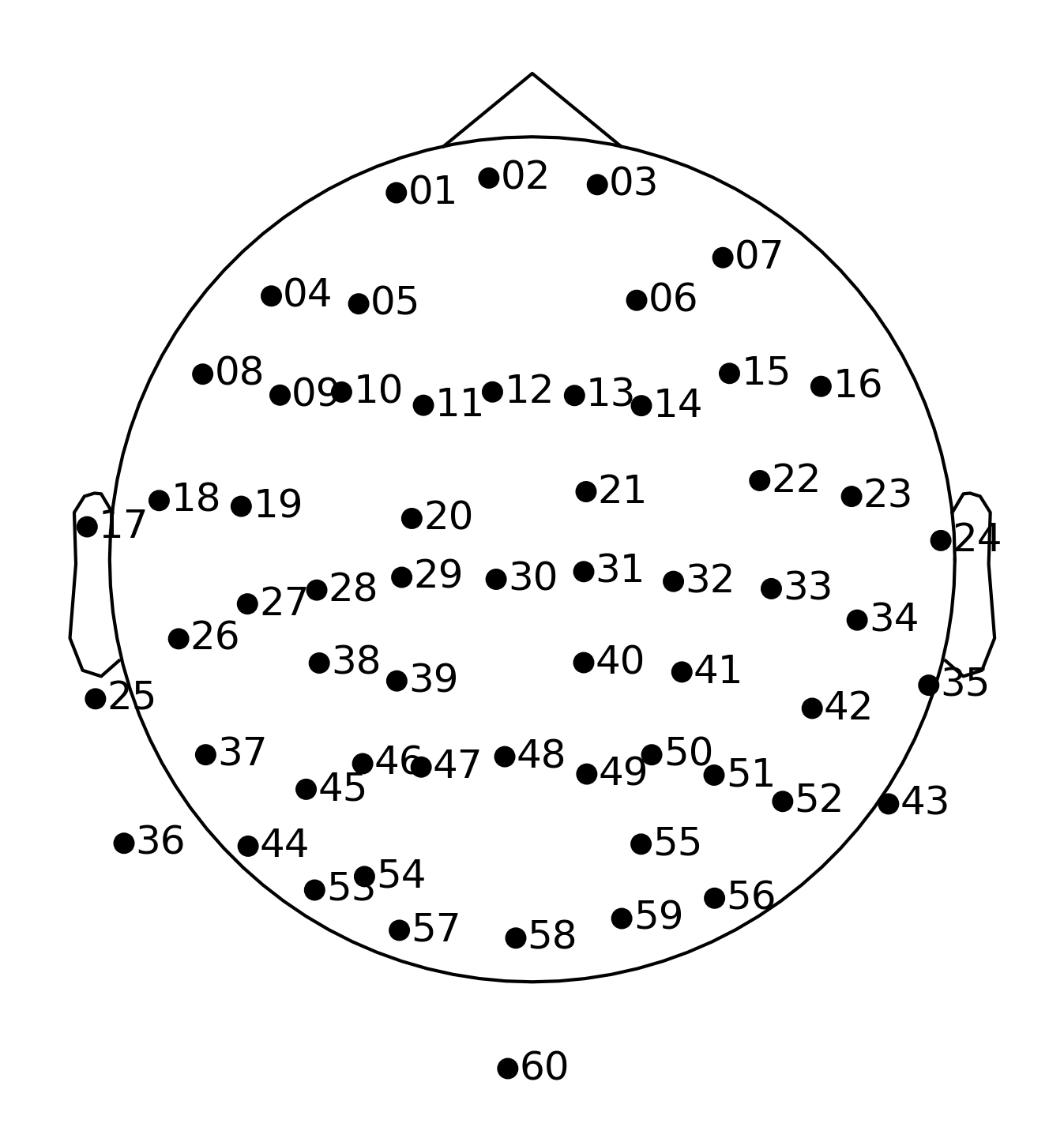
Figure 4: Montage displaying the standardized sensor positions of a sample subject used in the MNE dataset.

Table 1: Typical values of local parameters of Jansen-Rit parameters as used in TVB [43].

Parameter	Description	Typical Values (low, high)
$A_{e}$	Average excitatory synaptic gain	(2.6, 9.75) mV
$A_{i}$	Average inhibitory synaptic gain	(17.6, 110.0) mV
$b_{e}$	Inverse of time constant of excitatory postsynaptic potential	(0.050, 0.150) $s^{-1}$
$b_{i}$	Inverse of time constant of inhibitory postsynaptic potential	(0.025, 0.075) $s^{-1}$
$C$	Average number of synapses between the populations	135
$a_{1}$	Average number of synapses established by principal neurons on excitatory interneurons	(0.5, 1.5) × C
$a_{2}$	Average number of synapses established by excitatory interneurons on principal neurons	(0.4, 1.2) × C
$a_{3}$	Average number of synapses established by principal neurons on inhibitory interneurons	(0.125, 0.375) × C
$a_{4}$	Average number of synapses established by inhibitory interneurons on principal neurons	(0.125, 0.375) × C

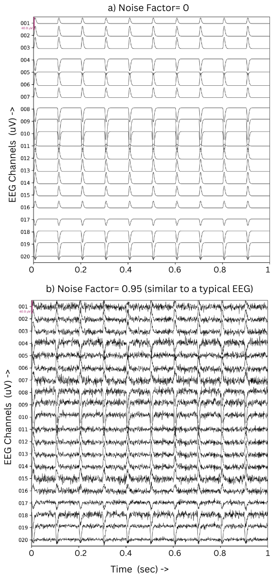
Figure 7: EEG simulated under two conditions: without added noise ((a) Noise Factor = 0) and (b) significant added noise, Noise Factor = 0.95, mimicking typical EEG). Each panel displays 20 EEG channels over a time span of one second.

References

- [1] Eric Bazin, Kevin J Dawson and Mark A Beaumont “Likelihood-free inference of population structure and local adaptation in a Bayesian hierarchical model” In Genetics 185.2 Oxford University Press, 2010, pp. 587–602
- [2] David Blei, Andrew Ng and Michael Jordan “Latent dirichlet allocation” In Advances in neural information processing systems 14, 2001
- [3] Caglar Cakan, Nikola Jajcay and Klaus Obermayer “neurolib: A simulation framework for whole-brain neural mass modeling” In Cognitive Computation 15.4 Springer, 2023, pp. 1132–1152
- [4] Filippo Cona et al. “A neural mass model of interconnected regions simulates rhythm propagation observed via TMS-EEG” In NeuroImage 57.3 Elsevier, 2011, pp. 1045–1058
- [5] Kyle Cranmer, Johann Brehmer and Gilles Louppe “The frontier of simulation-based inference” In Proceedings of the National Academy of Sciences 117.48 National Acad Sciences, 2020, pp. 30055–30062
- [6] FH Lopes Da Silva et al. “Models of neuronal populations: the basic mechanisms of rhythmicity” In Progress in brain research 45 Elsevier, 1976, pp. 281–308
- [7] Olivier David and Karl Friston “A Neural Mass Model for MEG/EEG: coupling and neuronal dynamics” In NeuroImage 20, 2003, pp. 1743–55 DOI: 10.1016/j.neuroimage.2003.07.015
- [8] Christophe Destrieux, Bruce Fischl, Anders Dale and Eric Halgren “Automatic parcellation of human cortical gyri and sulci using standard anatomical nomenclature” In Neuroimage 53.1 Elsevier, 2010, pp. 1–15
- [9] Conor Durkan, Iain Murray and George Papamakarios “On contrastive learning for likelihood-free inference” In International conference on machine learning, 2020, pp. 2771–2781 PMLR
- [10] Andrew Gelman and Jennifer Hill “Data analysis using regression and multilevel/hierarchical models” Cambridge University Press, 2006
- [11] Anubhab Ghosh, Mohamed Abdalmoaty, Saikat Chatterjee and Håkan Hjalmarsson “DeepBayes -an estimator for parameter estimation in stochastic nonlinear dynamical models”, 2022
- [12] Xavier Glorot and Yoshua Bengio “Understanding the difficulty of training deep feedforward neural networks” In International Conference on Artificial Intelligence and Statistics, 2010 URL: https://api.semanticscholar.org/CorpusID:5575601
- [13] Alexandre Gramfort et al. “MEG and EEG data analysis with MNE-Python” In Frontiers in neuroscience 7 Frontiers, 2013, pp. 70133
- [14] Alex Graves, Abdel-rahman Mohamed and Geoffrey Hinton “Speech recognition with deep recurrent neural networks” In 2013 IEEE international conference on acoustics, speech and signal processing, 2013, pp. 6645–6649 Ieee
- [15] David Greenberg, Marcel Nonnenmacher and Jakob Macke “Automatic posterior transformation for likelihood-free inference” In International Conference on Machine Learning, 2019, pp. 2404–2414 PMLR
- [16] David Greenberg, Marcel Nonnenmacher and Jakob Macke “Automatic posterior transformation for likelihood-free inference” In International Conference on Machine Learning, 2019, pp. 2404–2414 PMLR
- [17] John Griffiths et al. “Deep Learning-Based Parameter Estimation for Neurophysiological Models of Neuroimaging Data”, 2022 DOI: 10.1101/2022.05.19.492664
- [18] Paul Gustafson “Bayesian inference in partially identified models: Is the shape of the posterior distribution useful?”, 2014
- [19] Joeri Hermans, Volodimir Begy and Gilles Louppe “Likelihood-free mcmc with amortized approximate ratio estimators” In International conference on machine learning, 2020, pp. 4239–4248 PMLR
- [20] Sepp Hochreiter and Jürgen Schmidhuber “Long Short-term Memory” In Neural computation 9, 1997, pp. 1735–80 DOI: 10.1162/neco.1997.9.8.1735
- [21] Ben H. Jansen and Vincent G. Rit “Electroencephalogram and visual evoked potential generation in a mathematical model of coupled cortical columns” In Biological Cybernetics, 1995 DOI: https://doi.org/10.1007/BF00199471
- [22] Ileana O Jelescu, Marco Palombo, Francesca Bagnato and Kurt G Schilling “Challenges for biophysical modeling of microstructure” In Journal of Neuroscience Methods 344 Elsevier, 2020, pp. 108861
- [23] Levin Kuhlmann et al. “Neural mass model-based tracking of anesthetic brain states” In NeuroImage 133 Elsevier, 2016, pp. 438–456
- [24] Guoshi Li et al. “Multiscale neural modeling of resting-state fMRI reveals executive-limbic malfunction as a core mechanism in major depressive disorder” In NeuroImage: Clinical 31 Elsevier, 2021, pp. 102758
- [25] Gabriele Lohmann, Kerstin Erfurth, Karsten Müller and Robert Turner “Critical comments on dynamic causal modelling” In Neuroimage 59.3 Elsevier, 2012, pp. 2322–2329
- [26] FH Lopes da Silva, A Hoeks, H Smits and LH Zetterberg “Model of brain rhythmic activity: the alpha-rhythm of the thalamus” In Kybernetik 15 Springer, 1974, pp. 27–37
- [27] Carsten Mente et al. “Parameter estimation with a novel gradient-based optimization method for biological lattice-gas cellular automaton models” In Journal of mathematical biology 63, 2010, pp. 173–200 DOI: 10.1007/s00285-010-0366-4
- [28] Rosalyn Moran, Dimitris Pinotsis and Karl Friston “Neural Masses and Fields in Dynamic Causal Modelling” In Frontiers in computational neuroscience 7, 2013, pp. 57 DOI: 10.3389/fncom.2013.00057
- [29] George Papamakarios and Iain Murray “Fast -free Inference of Simulation Models with Bayesian Conditional Density Estimation” In Advances in Neural Information Processing Systems 29 Curran Associates, Inc., 2016, pp. 1028–1036 URL: http://papers.nips.cc/paper/6084-fast-free-inference-of-simulation-models-with-bayesian-conditional-density-estimation
- [30] David Papo “Time scales in cognitive neuroscience” In Frontiers in Physiology 4, 2013
- [31] Anagh Pathak, Dipanjan Roy and Arpan Banerjee “Whole-brain network models: from physics to bedside” In Frontiers in Computational Neuroscience 16 Frontiers, 2022, pp. 866517
- [32] Dimitris Pinotsis, Peter Robinson, Peter Beim Graben and Karl Friston “Neural Masses and Fields: Modelling the Dynamics of Brain Activity” In Frontiers in Computational Neuroscience 8, 2014 DOI: 10.3389/fncom.2014.00149
- [33] Petra Ritter, Michael Schirner, Anthony R McIntosh and Viktor K Jirsa “The virtual brain integrates computational modeling and multimodal neuroimaging” In Brain connectivity 3.2 Mary Ann Liebert, Inc. 140 Huguenot Street, 3rd Floor New Rochelle, NY 10801 USA, 2013, pp. 121–145
- [34] Pedro Rodrigues, Thomas Moreau, Gilles Louppe and Alexandre Gramfort “HNPE: Leveraging global parameters for neural posterior estimation” In Advances in Neural Information Processing Systems 34, 2021, pp. 13432–13443
- [35] Sadjad Sadeghi et al. “Dynamic causal modeling for fMRI with wilson-cowan-based neuronal equations” In Frontiers in Neuroscience 14 Frontiers, 2020, pp. 593867
- [36] Ruslan Salakhutdinov, Joshua B Tenenbaum and Antonio Torralba “Learning with hierarchical-deep models” In IEEE transactions on pattern analysis and machine intelligence 35.8 IEEE, 2012, pp. 1958–1971
- [37] Paula Sanz Leon et al. “The Virtual Brain: a simulator of primate brain network dynamics” In Frontiers in neuroinformatics 7 Frontiers Media SA, 2013, pp. 10
- [38] Paula Sanz-Leon, Stuart A Knock, Andreas Spiegler and Viktor K Jirsa “Mathematical framework for large-scale brain network modeling in The Virtual Brain” In Neuroimage 111 Elsevier, 2015, pp. 385–430
- [39] Fernando H. Silva, A Hoeks, H Smits and Lars H. Zetterberg “Model of brain rhythmic activity” In Kybernetik 15, 1974, pp. 27–37
- [40] Roberto C Sotero et al. “Realistically coupled neural mass models can generate EEG rhythms” In Neural computation 19.2 MIT Press, 2007, pp. 478–512
- [41] Leon Stefanovski et al. “Bridging scales in alzheimer’s disease: Biological framework for brain simulation with the virtual brain” In Frontiers in Neuroinformatics 15 Frontiers Media SA, 2021, pp. 630172
- [42] Yee Whye Teh and Michael I Jordan “Hierarchical Bayesian nonparametric models with applications” In Bayesian nonparametrics 1 Camb. Ser. Stat. Probab. Math, 2010, pp. 158–207
- [43] The Virtual Brain “Jansen and Rit model module”, 2024 URL: https://docs.thevirtualbrain.org/_modules/tvb/simulator/models/jansen_rit.html
- [44] Oscar Vilarroya “Neural Representation. A Survey-Based Analysis of the Notion” In Frontiers in Psychology 8, 2017 DOI: 10.3389/fpsyg.2017.01458
- [45] Fabrice Wendling, Pascal Benquet, Fabrice Bartolomei and Viktor Jirsa “Computational models of epileptiform activity” In Journal of neuroscience methods 260 Elsevier, 2016, pp. 233–251
- [46] Hugh Wilson and Jack Cowan “A Mathematical Theory of the Functional Dynamics of Cortical and Thalamic Nervous Tissue” In Kybernetik 13, 1973, pp. 55–80 DOI: 10.1007/BF00288786
- [47] Hugh R. Wilson and Jack D. Cowan “Excitatory and inhibitory interactions in localized populations of model neurons.” In Biophysical journal 12 1, 1972, pp. 1–24 URL: https://api.semanticscholar.org/CorpusID:17499302