ADBA:Approximation Decision Boundary Approach for Black-Box Adversarial Attacks

Abstract

Many machine learning models are susceptible to adversarial attacks, with decision-based black-box attacks representing the most critical threat in real-world applications. These attacks are extremely stealthy, generating adversarial examples using hard labels obtained from the target machine learning model. This is typically realized by optimizing perturbation directions, guided by decision boundaries identified through query-intensive exact search, significantly limiting the attack success rate. This paper introduces a novel approach using the Approximation Decision Boundary (ADB) to efficiently and accurately compare perturbation directions without precisely determining decision boundaries. The effectiveness of our ADB approach (ADBA) hinges on promptly identifying suitable ADB, ensuring reliable differentiation of all perturbation directions. For this purpose, we analyze the probability distribution of decision boundaries, confirming that using the distribution’s median value as ADB can effectively distinguish different perturbation directions, giving rise to the development of the ADBA-md algorithm. ADBA-md only requires four queries on average to differentiate any pair of perturbation directions, which is highly query-efficient. Extensive experiments on six well-known image classifiers clearly demonstrate the superiority of ADBA and ADBA-md over multiple state-of-the-art black-box attacks. The source code is available at https://github.com/BUPTAIOC/ADBA.

1 Introduction

Background and motivation. It is widely acknowledged that machine learning methods such as Deep Neural Networks (DNNs) are vulnerable to adversarial attacks [44, 43]. Particularly, for image classification tasks, tiny additive perturbations in the input images can significantly affect the classification accuracy of a pre-trained model [44]. The impact of these intentionally designed perturbations in real-world scenarios [12, 26] has heightened security worries for critical applications of deep neural networks in many domains [12, 24, 25, 23], which is detailed in Appendix A.

Adversarial attacks can be categorized into white-box attacks and black-box attacks [28]. White-box attacks [41] require the attacker to have comprehensive knowledge of the target machine learning model, rendering them impractical in many real-world scenarios. In comparison, black-box attacks [1, 2, 22] are more realistic since they do not required detailed knowledge of the target model.

Black-box attacks can be divided into transfer-based attacks, score-based attacks (or soft-label attacks, gray-box attacks), and decision-based attacks (hard-label attacks) [22]. More detailed discussion of these attacks can be found in Appendix B. Among them, decision-based attacks [2, 22, 35, 4, 9] are extremely stealthy since they rely solely on the hard label from the target model to create adversarial examples.

This paper studies the decision-based attacks due to their general applicability and effectiveness in real-world adversarial situations. These attacks aim to deceive the target model while adhering to two constraints [17]: 1) they must generate adversarial examples with as few queries as possible (i.e., query-efficient) and cannot exceed a predetermined number of queries (i.e., query budget), and 2) the strength of the adversarial perturbations must remain within a predefined threshold $\epsilon$. Violating those constrains results in the attack being easily detected or deemed unsuccessful. These constraints bring huge challenges to attackers [17]. Specifically, lacking detailed knowledge of the target model and its output scores poses tremendous difficulty for attackers to determine the decision boundary (i.e., the minimum perturbation strength required to deceive the model) with respect to any perturbation direction [9]. Thus, decision-based attacks often require a large number of queries to identify the decision boundary and optimize the perturbation direction, increasing the likelihood of being detected and hurting the attack success rate. Therefore, enhancing attack efficiency and minimizing the number of queries are essential for decision-based attacks [1, 4, 9, 17].

Proposed method. Existing decision-based attacks can be divided into random search attacks [2, 22, 9, 3, 5, 8](reviewed in detail in Section 2), gradient estimation attacks [4, 21, 27, 32], and geometric modeling attacks [42, 33, 29](reviewed in detail in Appendix B). This paper focuses on random search attacks, aiming to find the optimal perturbation direction with the smallest decision boundary. For this purpose, query-intensive exact search techniques such as binary search are typically utilized to identify the decision boundaries of different perturbation directions [9, 5]. For two candidate perturbation directions $\bm{d_{1}}$ and $\bm{d_{2}}$. Binary search is used to calculate their decision boundaries $g(\bm{d_{1}})$ and $g(\bm{d_{2}})$, and determine which direction has the smaller decision boundary [5]. However, binary search demands for a large number of queries, resulting in poor query efficiency.

In this study, we show that different perturbation directions can be compared without knowing their precise decision boundaries, avoiding costly exact search methods, as demonstrated in Figure LABEL:Fig1.sub.3. Suppose that an approximation decision boundary (ADB) enables direction $\bm{d_{2}}$ to deceive the target model but direction $\bm{d_{1}}$ fails to do the same, we can conclude that $g(\bm{d_{2}})\leq\text{ADB}<g(\bm{d_{1}})$ and $\bm{d_{2}}$ is deemed superior for the black-box attack. Here, $g(\bm{d_{1}})\text{and }g(\bm{d_{2}})$ refer to the actual decision boundaries of $\bm{d_{1}}\text{and }\bm{d_{2}}$. On the contrary, $g(\bm{d_{1}})$ and $g(\bm{d_{2}})$ cannot be clearly differentiated upon using ADB that is either too large or too small, as shown in Figure LABEL:Fig1.sub.1 and Figure LABEL:Fig1.sub.2. Hence, a key issue is to quickly find an appropriate ADB with few queries. To tackle this issue, we analyze the probability distribution of decision boundaries and discover that it is highly likely for any pair of perturbation directions to be successfully differentiated upon using this distribution’s median value as ADB. In fact, only four queries on average are required for this purpose. Based on this idea, we propose innovative Approximation Decision Boundary Approach (ADBA) and Median-Search Based ADBA (ADBA-md) for random search attacks.

Comprehensive experiments. We perform comprehensive experiments for decision-based black-box attacks using a variety of image classification models. We select 6 well-known deep models that span a wide range of architectures. We compare our methods with four state-of-the-art decision-based adversarial attack approaches. The results show that our methods can generate adversarial examples with a high attack success rate (i.e., fooling rate) while using a small number of queries.

This paper makes three main contributions. (1) We propose a novel Approximation Decision Boundary Approach (ADBA) for query-efficient decision-based attacks. (2) We analyze the distribution of decision boundaries and discover that using the distribution’s median value as ADB can differentiate any pair of perturbation directions with high query efficiency, giving rise to the development of ADBA-md. (3) We conduct comprehensive experiments, demonstrating that ADBA and ADBA-md can significantly outperform four leading decision-based attack approaches across six modern deep models on the ImageNet dataset.

2 Related work

Random search attacks adopt a random search framework to generate candidate perturbation directions and adjust them according to the sizes of decision boundaries. [2, 3, 8, 9, 5]. These boundaries are precisely identified through methods such as binary search, which requires a large number of queries. For example, Boundary Attack [2], Biased Boundary Attack [3], and AHA [22] progressively alter the current perturbation direction through a random walk along the decision boundary, which is query-intensive. To reduce the number of queries in [2], Biased Boundary Attack [3] proposes a biased sampling framework to accelerate the search for perturbation directions. Meanwhile, AHA in [22] gathers information from all historical queries as a prior for current sampling decisions to improve the efficiency of random walk. Additionally, OPT and Sign-OPT developed respectively in [8] and [9] transform the hard-label black-box attack to a continuous optimization problem, solvable through zeroth-order optimization. However, they utilize binary search to identify the decision boundary of each perturbation direction, demanding for a large number of queries. RayS in [5] is a state-of-the-art decision-based attack based on the $l_{\infty}$ norm. It transforms the task of optimizing the perturbation direction from the continuous domain to the discrete domain. It generates perturbation directions by progressively dividing and inverting direction vectors, with each division resulting in smaller blocks as the optimization advances, noticeably enhancing the efficiency in finding good directions. However, RayS optimizes perturbation directions based on precise estimation of the decision boundary through a query-intensive binary search process. More discussion of related works, including gradient estimation attacks and geometric modeling attacks, can be found in Appendix B.

3 Proposed Method

3.1 Preliminaries

Let $F\colon\mathbb{X}^{N}\rightarrow\{1,\dots,K\}$ denote a target image classification model that assigns images to one of $K$ distinct classes. The model’s input is a normalized RGB image $\bm{x}\in\mathbb{X}^{N}$, where $N=\text{Width}\times\text{Height}\times\text{Channels}$ represents the dimensionality of the image, encompassing all pixels across all channels. In this context, $\mathbb{X}^{N}$ is the input space of all images to be classified. The channel value of each pixel of any image $\bm{x}\in\mathbb{X}^{N}$ ranges between 0 and 1. Meanwhile, $y(\bm{x})\in\{1,\dots,K\}$ denotes the true label of image $\bm{x}$, and $F(\bm{x})$ is the label produced by the classification model $F$ for image $\bm{x}$. The goal of an adversarial attack is to find an adversarial example $\tilde{\bm{x}}\in\mathbb{X}^{N}$ such that $F(\tilde{\bm{x}})\neq y(\bm{x})$ (untargeted attack) or $F(\tilde{\bm{x}})=t$ (targeted attack, where $t$ is a given target label, and $t\neq y(\bm{x})$), subject to the condition that $\|\tilde{\bm{x}}-\bm{x}\|_{v}\leq\epsilon$, where $\bm{x}$ is a correctly classified image. Here, $\epsilon$ refers to the allowed maximum perturbation strength and $v$ refers to the norm used to measure the perturbation strength, such as $l_{1}$, $l_{2}$, and $l_{\infty}$ norms [28]. In this paper, we adopt the $l_{\infty}$ norm, following RayS [5]. This paper focuses primarily on untargeted attacks, aiming to force the target image classification models to produce arbitrary incorrect class labels for any image $\bm{x}$. This goal can be expressed as follows:

$$\max_{\tilde{\bm{x}}}f(\bm{x},y(\bm{x}),\tilde{\bm{x}})\quad\text{subject to}\quad\|\tilde{\bm{x}}-\bm{x}\|_{\infty}\leq\epsilon$$ (1)

$$\text{where}\quad f(\bm{x},y(\bm{x}),\tilde{\bm{x}})=\begin{cases}0&\text{if }F(\tilde{\bm{x}})\neq y(\bm{x})\\ -1&\text{if }F(\tilde{\bm{x}})=y(\bm{x})\end{cases}$$

Let the adversarial perturbation $\tilde{\bm{x}}-\bm{x}=r\cdot\bm{d}$, where $\bm{d}\in[-1,1]^{N}$ represents the perturbation direction and $r\in[0,\epsilon]$ represents the perturbation strength. Prior works [17, 5, 8, 30, 6], proved that the optimal solution to question (1) is at the extremities of the $\ell_{\infty}$ norm ball, i.e., $\bm{d}\in\{-1,1\}^{N}$. In this case, $\|\tilde{\bm{x}}-\bm{x}\|_{\infty}=\|r\cdot\bm{d}\|_{\infty}=r\cdot\|\bm{d}\|_{\infty}=r$. Hence, the continuous optimization problem in question (1) is transformed into a mixed-integer optimization problem according to [5]:

$$\max_{r\in[0,\epsilon],\bm{d}\in\{-1,1\}^{N}}h(\bm{x},y(\bm{x}),r,\bm{d})\quad$$

$$\text{where}\quad h(\bm{x},y(\bm{x}),r,\bm{d})=\begin{cases}0&\text{if }F(\bm{x}+r\cdot\bm{d})\neq y(\bm{x})\\ -1&\text{if }F(\bm{x}+r\cdot\bm{d})=y(\bm{x})\end{cases}$$

Previous works [9, 17, 5, 8] also proved that the solution space of question (3.1) is continuous, and exploited the concept of the decision boundary to develop effective adversarial attacks. For any direction $\bm{d}$, there exists a decision boundary $g(\bm{d})$ such that $F(\bm{x}+g(\bm{d})\cdot\bm{d})\neq y(\bm{x})$ and $F(\bm{x}+(g(\bm{d})-\Delta)\cdot\bm{d})=y(\bm{x})$, $\forall\Delta\in(0,\tau]$. $g(\bm{d})$ is further defined in question (3.1) below. As shown in Figure LABEL:Fig1.sub.1, $g(\bm{d_{\text{best}}})$, $g(\bm{d_{1}})$, and $g(\bm{d_{2}})$ are the decision boundaries of the previous best direction $\bm{d_{\text{best}}}$ and two new candidate directions $\bm{d_{1}}$, $\bm{d_{2}}$, respectively. According to the definition of current decision boundary in [5], the decision-based attacks have the goal to find the optimal perturbation direction $\bm{d_{\text{best}}}$:

$$\bm{d_{\text{best}}}=\operatorname*{argmin}_{\bm{d}\in\{-1,1\}^{N}}g(\bm{d})\quad\text{with}\quad g(\bm{d})=\inf\{F(\bm{x}+r\cdot\bm{d})\neq y(\bm{x})\}$$

According to the above equation, the direction $\bm{d_{2}}$ in Figure LABEL:Fig1.sub.1 has the smallest decision boundary $g(\bm{d_{2}})$ among $g(\bm{d_{\text{best}}})$, $g(\bm{d_{1}})$, and $g(\bm{d_{2}})$.

Algorithm 1 Approximate Decision Boundary Approach

Input: Model $F$, the original image $\bm{x}$ and its label $y(\bm{x})$, and maximum perturbation strength $\epsilon$;
Output: Optimal direction $\bm{d_{\text{best}}}$ with approximation decision boundary $r_{\text{best}}$;
Initialization: Initialize current best direction $\bm{d_{\text{best}}}\leftarrow(1,\ldots,1)$, and set current best perturbation strength $r_{\text{best}}\leftarrow 1$, block variable $\leftarrow 0$ and block index $k\leftarrow 0$;

1:while remaining query budget $>0$ and $r_{\text{best}}>\epsilon$ do

2:     $L=N/2^{(s+1)}$;

3:     $\bm{d_{1}}\leftarrow\bm{d_{\text{best}}}$, $\bm{d_{2}}\leftarrow\bm{d_{\text{best}}}$;

4:     for $i\in[k\cdot L,(k+1)\cdot L)$ do

5:         $\bm{d_{1}}[i]\leftarrow-\bm{d_{1}}[i]$

6:     end for

7:     for $i\in[(k+1)\cdot L,(k+2)\cdot L)$ do

8:         $\bm{d_{2}}[i]\leftarrow-\bm{d_{2}}[i]$

9:     end for

10:     $\bm{d_{\text{best}}},r_{\text{best}}\leftarrow\text{Algorithm 2}(F,\{\bm{x},y(\bm{x})\},\bm{d_{\text{best}}},r_{\text{best}},\bm{d_{1}},\bm{d_{2}})$;

11:     $k\leftarrow k+2$;

12:     if $k=2^{(s+1)}$ then

13:         $s\leftarrow s+1$

14:         $k\leftarrow 0$

15:     end if

16:end while

17:return $\bm{d_{\text{best}}},r_{\text{best}}$

3.2 Approximation Decision Boundary Approach (ADBA)

To compare the decision boundary $g(\bm{d})$ of different directions, existing methods typically employ exact search techniques such as binary search [9][17] [5] to identify $g(\bm{d})$ with high accuracy (e.g., up to 0.001 [5]). Obviously, this process requires a large number of queries. We notice that, in the early stages of optimization, directions are often far away from optima and their decision boundaries often exceed the threshold $\epsilon$ on the perturbation strength. Thus it is unnecessary to precisely identify the decision boundary. However, existing works [8, 9, 5] perform numerous queries to determine the accurate decision boundary, even in the early stages, resulting in poor query efficiency. Different from these works, in this paper, we demonstrate that perturbation directions can be reliably compared and optimized without knowing the precise decision boundary. Driven by this idea, we propose ADBA, as summarized in Algorithm 1.

In Algorithm 1, ADBA iteractively searches for the optimal perturbation direction. It keeps track of the current best direction $\bm{d_{\text{best}}}$ along with its ADB $r_{\text{best}}$ , and update $\bm{d_{\text{best}}}$ and $r_{\text{best}}$ in each iteration. The initial perturbation direction $\bm{d_{\text{best}}}$ is flattened into a one-dimensional vector $(1,\ldots,1)$ with $N=\text{Width}\times\text{Height}\times\text{Channels}$ dimensions. The current best perturbation strength $r_{\text{best}}$ that represents the ADB of $\bm{d_{\text{best}}}$ is set to 1 initially to make sure that $F(\bm{x}+r_{\text{best}}\cdot\bm{d_{\text{best}}})\neq y(\bm{x})$. In line with RayS [5], we use the block variable $s$ to control the block size. In line 2, the current best direction vector $\bm{d_{\text{best}}}$ is divided into $2^{(s+1)}$ smaller blocks. In lines 3-9 of each algorithm iteration, we choose two blocks of $\bm{d_{\text{best}}}$ in sequence and reverse the sign of each block respectively to create two new directions, $\bm{d_{1}}$ and $\bm{d_{2}}$. In line 10, different from [5] that uses binary search to accurately identify $g(\bm{d_{1}})$ and $g(\bm{d_{2}})$, we devise Algorithm 2 (to be detailed in Subsection 3.2.1) to update the optimal direction $\bm{d_{\text{best}}}$ based on its approximation decision boundary $r_{\text{best}}$. In lines 11-15, if the block index $k$ reaches $2^{(s+1)}$, i.e., all current blocks have been utilized for reversal, then $2^{(s+2)}$ more directions are produced in subsequent iterations by $s\leftarrow s+1$. If the ADB $r_{\text{best}}$ of $\bm{d_{\text{best}}}$ is within the allowed strength $\epsilon$ or the number of queries exceeds the budget, Algorithm 1 returns the current best direction together with its perturbation strength. The former scenario indicates a successful attack, while the latter signifies a failed attack.

Algorithm 2 Compare Directions Using ADB

Input: Model $F$, original image $\bm{x}$ and its label $y(\bm{x})$, current best direction $\bm{d_{\text{best}}}$ with approximation decision boundary $r_{\text{best}}$, two new directions $\bm{d_{1}}$, $\bm{d_{2}}$, and search tolerance $\tau$;
Output: New best direction $\bm{d_{\text{best}}}$ with approximation decision boundary $r_{\text{best}}$
Initialization: Set $\text{ADB}\leftarrow r_{\text{best}}$, start $\leftarrow 0$, end $\leftarrow r_{\text{best}}$

1:if $F(\bm{x}+r_{\text{best}}\cdot\bm{d_{1}})=y(\bm{x})$ and $F(\bm{x}+r_{\text{best}}\cdot\bm{d_{2}})=y(\bm{x})$ then

2:     return $\bm{d_{\text{best}}},r_{\text{best}}$

3:end if

4:while end - start $>\tau$ do

5:     if $F(\bm{x}+\text{ADB}\cdot\bm{d_{1}})\neq y(\bm{x})$ and $F(\bm{x}+\text{ADB}\cdot\bm{d_{2}})\neq y(\bm{x})$ then

6:         $\text{ADB}\leftarrow(\textit{start}+\textit{end})/2$

7:         end $\leftarrow\text{ADB}$

8:     else if $F(\bm{x}+\text{ADB}\cdot\bm{d_{1}})=y(\bm{x})$ and $F(\bm{x}+\text{ADB}\cdot\bm{d_{2}})=y(\bm{x})$ then

9:         $\text{ADB}\leftarrow(\textit{start}+\textit{end})/2$

10:         start $\leftarrow\text{ADB}$

11:     else if $F(\bm{x}+\text{ADB}\cdot\bm{d_{1}})\neq y(\bm{x})$ and $F(\bm{x}+\text{ADB}\cdot\bm{d_{2}})=y(\bm{x})$ then

12:         return $\bm{d_{1}},\text{ADB}$

13:     else if $F(\bm{x}+\text{ADB}\cdot\bm{d_{1}})=y(\bm{x})$ and $F(\bm{x}+\text{ADB}\cdot\bm{d_{2}})\neq y(\bm{x})$ then

14:         return $\bm{d_{2}},\text{ADB}$

15:     end if

16:end while

17:return $\bm{d_{1}},\text{ADB}$

3.2.1 Comparing Perturbation Directions Using ADB

In this section, we propose a query-efficient method by comparing perturbation directions using ADB, rather than using binary search in [5]. Our idea is described in more details below. First, we determine whether $\bm{d_{1}}$ and $\bm{d_{2}}$ are superior to $\bm{d_{\text{best}}}$; if not, $\bm{d_{\text{best}}}$ remains the current best, and there is no need to compare $\bm{d_{1}}$ and $\bm{d_{2}}$. We denote the ADB $r_{\text{best}}$ of $\bm{d_{\text{best}}}$ as $\text{ADB}_{1}$ and check whether both $F(\bm{x}+\text{ADB}_{1}\cdot\bm{d_{1}})$ and $F(\bm{x}+\text{ADB}_{1}\cdot\bm{d_{2}})$ produce wrong class labels (attacks are successful). If $\text{ADB}_{1}$ is too large and both attacks succeed, as shown in Figure LABEL:Fig1.sub.1, then $g(\bm{d_{1}})\leq\text{ADB}_{1}$ and $g(\bm{d_{2}})\leq\text{ADB}_{1}$. In this case, we cannot differentiate $g(\bm{d_{1}})$ and $g(\bm{d_{2}})$. Hence, ADB is decreased to $\text{ADB}_{2}=(0+\text{ADB}_{1})/2$. Subsequently, we check whether $F(\bm{x}+\text{ADB}_{2}\cdot\bm{d_{1}})$ and $F(\bm{x}+\text{ADB}_{2}\cdot\bm{d_{2}})$ can lead to incorrect classification. If $\text{ADB}_{2}$ is too small and both attacks fail, as demonstrated in Figure LABEL:Fig1.sub.2, $g(\bm{d_{1}})>\text{ADB}_{2}$ and $g(\bm{d_{2}})>\text{ADB}_{2}$. In this case, we still cannot differentiate $g(\bm{d_{1}})$ and $g(\bm{d_{2}})$. We instead increase ADB to $\text{ADB}_{3}=(\text{ADB}_{2}+\text{ADB}_{1})/2$, and check whether $F(\bm{x}+\text{ADB}_{3}\cdot\bm{d_{1}})$ and $F(\bm{x}+\text{ADB}_{3}\cdot\bm{d_{2}})$ can induce wrong classification. This time, in Figure LABEL:Fig1.sub.3, the attack along the direction $\bm{d_{2}}$ succeeds, and the attack along the direction $\bm{d_{1}}$ fails, indicating $g(\bm{d_{2}})\leq\text{ADB}_{3}<g(\bm{d_{1}})$; i.e., $\bm{d_{2}}$ is superior to $\bm{d_{1}}$. Subsequently, we update $\bm{d_{\text{best}}}=\bm{d_{2}}$, $r_{\text{best}}=\text{ADB}_{3}$.

The above process is summarized in Algorithm 2. Notably, for the current best direction $\bm{d_{\text{best}}}$ in Figure LABEL:Fig1.sub.1, because its real decision boundary $g(\bm{d_{\text{best}}})\leq r_{\text{best}}$, we cannot compare $g(\bm{d_{\text{best}}})$ and $g(\bm{d_{2}})$. However, further comparison of $\bm{d_{\text{best}}}$ and $\bm{d_{2}}$ is unnecessary, since this requires twice as many queries with minimal improvement of $g(\bm{d_{\text{best}}})$, as evidenced by our preliminary experiments in Appendix C.

In Algorithm 2, ADB is set initially to the ADB of the current best direction $\bm{d_{\text{best}}}$. In lines 1 and 2, if $g(\bm{d_{\text{best}}})\leq r_{\text{best}}<g(\bm{d_{1}})$ and $g(\bm{d_{\text{best}}})\leq r_{\text{best}}<g(\bm{d_{2}})$ (i.e., $\bm{d_{1}}$ and $\bm{d_{2}}$ are worse than $\bm{d_{\text{best}}}$), it is worthless to perform further comparisons. Algorithm 2 hence returns $\bm{d_{\text{best}}}$ as its output. In lines 5 to 10, if the decision boundaries of $\bm{d_{1}}$ and $\bm{d_{2}}$ are both either smaller or larger than ADB, then Algorithm 2 updates the start or end to narrow the search range for ADB. In lines 11 to 14, if the current ADB leads to a successful attack in one direction but not the other direction, Algorithm 2 reports the successful direction and the corresponding ADB. In line 17, if the search range end - start is less than a search tolerance threshold $\tau$, indicating that $g(\bm{d_{1}})$ and $g(\bm{d_{2}})$ are closely matched, the algorithm returns $\bm{d_{1}}$ along with the current ADB. Meanwhile, according to Appendix C, it is unnecessary to compare $\bm{d_{1}}$ with $\bm{d_{\text{best}}}$ because this comparison requires an excessive number of queries while yielding minimal improvement to $g(\bm{d_{\text{best}}})$.

3.2.2 Optimization of ADB

The practical efficiency of Algorithm 2 depends on the swift identification of ADB that can differentiate any two directions $\bm{d_{1}}$ and $\bm{d_{2}}$ accurately. In lines 6 and 9 of Algorithm 2, if the current ADB fails to differentiate the two directions, the next search point is chosen as the middle point of the search range $[start,end]$, i.e., ADB $\leftarrow$ $(start+end)/2$. However, this simple method cannot achieve the desired query efficiency. In this paper, by considering the statistical distribution of decision boundaries, we can identify a more suitable ADB to improve the likelihood of differentiating $\bm{d_{1}}$ and $\bm{d_{2}}$. Based on this idea, we propose ADBA-md in this section.

We define the random events $A$, $B$, $C$ and $D$ as follows:

$$\begin{cases}A&=\{F(\bm{x}+\text{ADB}\cdot\bm{d_{1}})\neq y(\bm{x})\}=\{g(\bm{d_{1}})\leq\text{ADB}\}\\ B&=\{F(\bm{x}+\text{ADB}\cdot\bm{d_{2}})\neq y(\bm{x})\}=\{g(\bm{d_{2}})\leq\text{ADB}\}\\ C&=\{F(\bm{x}+\text{ADB}\cdot\bm{d_{1}})=y(\bm{x})\}=\{g(\bm{d_{1}})>\text{ADB}\}\\ D&=\{F(\bm{x}+\text{ADB}\cdot\bm{d_{2}})=y(\bm{x})\}=\{g(\bm{d_{2}})>\text{ADB}\}\end{cases}$$ (4)

We assume that $g(\bm{d_{1}})$ and $g(\bm{d_{2}})$ are independent random variables that follow an identical probability distribution $\rho$. The eligibility of adopting this assumption is clarified in Appendix D. The probability $P(A),P(B),P(C),P(D)$ for any $\text{ADB}\in[start,end]$ can be calculated respectively by:

$$\begin{cases}P(A)=P(B)=a=\int_{start}^{\text{ADB}}\rho(r)\,dr\\ P(C)=P(D)=b=\int_{\text{ADB}}^{end}\rho(r)\,dr\end{cases}$$ (5)

Accordingly, $P(B\cap C)=P(B)\cdot P(C\mid B)$ gives the probability of $g(\bm{d_{2}})\leq\text{ADB}<g(\bm{d_{1}})$, as illustrated in Figure LABEL:Fig1.sub.3. To avoid the complexity of determining $P(C\mid B)$, which requires extra queries, $g(\bm{d_{1}})$ and $g(\bm{d_{2}})$ are assumed to be independent. Therefore,

$$\begin{cases}P(B\cap C)=P(B)\cdot P(C\mid B)=P(B)\cdot P(C)=ab\\ P(A\cap D)=P(A)\cdot P(D\mid A)=P(A)\cdot P(D)=ab\\ P(A\cap B)=P(A)\cdot P(B\mid A)=P(A)\cdot P(B)=a^{2}\\ P(C\cap D)=P(C)\cdot P(D\mid C)=P(C)\cdot P(D)=b^{2}\\ \end{cases}$$ (6)

Consequently, in each comparison attempt, the probability $P({SUCC})$ for ADB to successfully differentiate a pair of directions $\bm{d_{1}}$ and $\bm{d_{2}}$ and the probability $P({FAIL})$ for ADB to fail to do so are determined respectively by:

$$\begin{cases}P({SUCC})=P(B\cap C)+P(A\cap D)=2ab,\\ P({FAIL})=P(A\cap B)+P(C\cap D)=a^{2}+b^{2}\end{cases}$$ (7)

$$\text{with }P({SUCC})+P({FAIL})=a^{2}+b^{2}+2ab=1\text{\ and\ }a+b=1$$

$P({SUCC})$ reaches its maximum by setting $a=b=0.5$, resulting in $P({SUCC})=P({FAIL})=1/2$. Hence, according to Eqn. (5), ADB should be set to divide the probability density function $\rho(r)$ into two parts of equal size, instead of setting ADB to $(start+end)/2$ at lines 6 and 9 in Algorithm 2. Specifically, we can set ADB to satisfy the following equation, without querying the target model:

$$\int_{start}^{\text{ADB}}\rho(r)\,dr=\int_{\text{ADB}}^{end}\rho(r)\,dr=\frac{1}{2}\cdot\int_{start}^{end}\rho(r)\,dr$$ (8)

Especially, if the probability distribution is uniformly identical, then ADB should be set to the mid point between $start$ and $end$. The expected number of queries required for differentiating any pair of perturbation directions can be kept small. In fact, it is straightforward to show that $P({SUCC})=1/2$. If differentiation fails in one comparison attempt, in the next attempt, Algorithm 2 updates $start$ and $end$ according to lines 7 and 10, and then sets ADB to satisfy Eqn. (8). Hence, $P(SUCC))$ remains to be $1/2$. Assuming that differentiation succeeds after $C$ comparison attempts, which means that the first $C-1$ comparison attempts fail and the $C$-th comparison attempt succeeds, the probability that $C$ equals any given $n$ is: $P(C=n)=(P({FAIL}))^{n-1}\cdot P({SUCC})=a^{n-1}\cdot b=\left(\frac{1}{2}\right)^{n}$. Hence, the expected number of comparison attempts $\bar{C}$ can be determined as $\bar{C}=1\cdot\left(\frac{1}{2}\right)^{1}+2\cdot\left(\frac{1}{2}\right)^{2}\cdot\cdot\cdot+n\cdot\left(\frac{1}{2}\right)^{n}=\sum_{n=1}^{\infty}n\cdot\left(\frac{1}{2}\right)^{n}=2$. Therefore, 2 consecutive guesses of ADB on average are required to differentiate a pair of directions. Meanwhile, for each comparison attempt, a total of 2 queries are performed using the perturbations ADB$\cdot\bm{d_{1}}$ and ADB$\cdot\bm{d_{2}}$ respectively in line 1, 5, 8, 11, and 13 of Algorithm 2. In total, the average number of queries required to differentiate any two directions is $\bar{Q}=2\times\bar{C}=2\times 2=4$.

Since Eqn. (6) is obtained by assuming that $g(\bm{d_{1}})$ and $g(\bm{d_{2}})$ are independent, the actual number of queries required to differentiate any two directions may not be $4$. However, the experiment results in Subsection 4.2 show that the number of queries achieved by ADBA is very close to $4$ in practice. Compared with RayS [5] that requires on average $10$ queries to reach an accuracy level of $0.001\approx 2^{\text{-10}}$ through binary search in our experiments, ADBA can noticeably reduce the required number of queries by approximately 2.5 times.

In Appendix D , in order to estimate the probability density function $\rho$, we conduct a statistical analysis of the distribution of the actual decision boundaries $r_{\text{best}}$, $g(\bm{d_{1}})$ and $g(\bm{d_{2}})$ under various settings of $\bm{d_{\text{best}}}$, $\bm{d_{1}}$ and $\bm{d_{2}}$. Subsequently, we utilize an inverse proportional function, i.e., $\rho(r)=\frac{a}{(|-r/r_{\text{best}}+d|)^{b}+c}$, $r\in[0,r_{\text{best}}]$, to estimate the true distribution of the decision boundary, where $a$, $b$, $c$, and $d$ are the estimation parameters. Specifically, $r_{\text{best}}$ is the ADB of the current best direction $\bm{d_{\text{best}}}$, which serves as the input of Algorithm 2. The efficiency of ADBA-md is insensitive to the accuracy of $\rho(r)$. Hence, ADBA-md can be easily applied to other datasets and target models, as supported by more experiment results reported in Appendix E. ADBA and ADBA-md do not incorporate random factors in Algorithm 1 and 2. Therefore, for the same original image, ADBA and ADBA-md will consistently generate the same adversarial examples across multiple repeated experiments.

4 Experiments

4.1 Experiment Settings

In this section, we conduct comprehensive experiments to compare ADBA and ADBA-md against several state-of-the-art decision-based attack approaches, including OPT [8], SignOPT [9], HSJA [4], and RayS [5]. Our experiments are conducted on a server with an Intel Xeon Gold 6330 CPU, NVIDIA 4090 GPUs using PyTorch 2.3.0, Torchvision 0.18.0 on the Python 3.11.5 platform.

Datasets and target models. We evaluate the performance of ADBA and ADBA-md on the ImageNet dataset [10], where each image in this dataset is resized to $224\times 224\times 3$ as a common practice [5]. The dataset is under BSD 3-Clause License. Our evaluation includes six contemporary machine learning models that are commonly used as attack target models [5, 9, 22, 33]: VGG19 [36], ResNet50 [15], Inception-V3 [37], ViT-B32 [11], DenseNet161 [16], and EfficientNet-B0 [38]. These models are implemented through the torchvision.models package in Python. We adopted the latest model weights retrievable from https://download.pytorch.org/models/: vgg19-dcbb9e9d.pth, resnet50-11ad3fa6.pth, inception_v3_google-0cc3c7bd.pth, vit_b_32-d86f8d99.pth, efficientnet_b0_rwightman-7f5810bc.pth, and densenet161-8d451a50.pth.

Attack settings. Following cutting-edge research on black-box adversarial attacks [5, 30], we adopt the $l_{\infty}$ norm and set the perturbation strength threshold $\epsilon=0.05$. Meanwhile, the query budget is set to 10000 for each model [5]. The parameters in the distribution function $\rho(r)=\frac{a}{(|-r/r_{\text{best}}+d|)^{b}+c}$, $r\in[0,r_{\text{best}}]$ are set to be $a=0.0313$, $b=3.066$, $c=0.168$, and $d=1.134$ according to Appendix D. The search tolerance threshold $\tau=0.002$.

Table 1: Comparison of decision-based untargeted attacks on the ImageNet dataset with 10,000 query budgets and maximum $l_{\infty}$ perturbation strengths $\epsilon=0.05$

Model	VGG	ResNet	Inception	ViT	DenseNet	EfficientNet
Attack	19	50	-V3	-B32	161	-B0
OPT	1473.0	2096.8	2213.6	3291.7	3373.6	2825.4
	(1191)	(1387)	(1419)	(2158)	(2350)	(1813)
	25.1%	9.2%	18.1%	16.2%	12.9%	10.8%
SignOPT	2575.2	3042.3	2253.3	3499.4	3943.7	3031.9
	(1765)	(1727)	(1337)	(1969)	(3051)	(1897)
	42.5%	22.5%	35.0%	30.8%	25.2%	17.6%
HSJA	589.1	1220.0	733.6	996.9	1891.0	1728.3
	(324)	(401)	(358)	(422)	(812)	(559)
	29.5%	12.7%	21.9%	18.8%	16.1%	13.9%
RayS	470.1	1243.5	672.2	1005.1	733.6	669.7
	(295)	(721)	(339)	(414)	(358)	(321)
	100%	98.8%	98.8%	98.8%	99.1%	99.8%
ADBA	237.3	769.3	461.3	768.4	485.7	428.3
	(119)	(339)	(156)	(221)	(158)	(143)
	100%	97.9%	99.4%	98.8%	99.2%	99.6%
ADBA-md	197.6	685.6	418.3	651.9	457.8	343.2
	(115)	(273)	(149)	(202)	(149)	(146)
	100%	99.3%	99.7%	99.8%	99.7%	99.8%

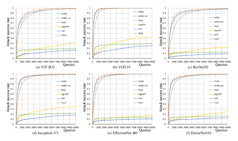
Figure 3: Attack success rates versus number of queries for six hard-label attacks on ImageNet.

4.2 Experiment Results

For six pre-trained models, we randomly select 1,000 correctly classified images from the ImageNet test set for each model. Then we produce adversarial examples for each image by using six hard-label attacks respectively to determine the attack success rate, which is calculated by $\frac{|E_{\text{successful}}|}{|E|}$. Here, $E$ refers to the set of all test cases ($|E|=1000$) and $E_{\text{successful}}$ is the set of successful attacks that meet the requirements for the query budget (i.e., 10000) and the perturbation strength threshold (i.e., $\epsilon=0.05$). In Table 1, we summarize the attack success rate and the average (median) number of queries for six attack methods across six target models. ADBA-md provides the highest attack success rate, exceeding 99.3% across all target models, and requires the fewest average number of queries across six black-box attacks. ADBA method results in the smallest median number of queries on the EfficientNet-B0 model, and ADBA-md has the smallest median number of queries on other models. Compared to other attack strategies, our methods significantly reduce the average number of queries to below 800 and the median number of queries to below 400.

Under similar attack success rates, both ADBA and ADBA-md can significantly reduce the average and median number of queries compared to RayS. Specifically, the average number of queries is approximately 60-70% of those required by RayS, and the median is reduced by 50%. Our results indicate that it is unnecessary to perform precise binary search as in RayS. Instead, it is much more efficient to optimize perturbation directions by using approximation decision boundaries.

Figure 3 presents a comparative performance analysis of six black-box methods on six target models, focusing on the attack success rate relative to the number of queries. ADBA and ADBA-md consistently achieve the highest attack success rates compared to other approaches. Notably, even with a very low query budget (1000 queries), both ADBA and ADBA-md attain an attack success rate of approximately 90%, whereas RayS achieves around 80%. The remaining three attack methods fail to obtain an attack success rate above 30%. This result confirms that our methods can achieve substantially higher success rate, making them highly effective under restricted query budgets.

Table 2: The Average number of iterations and queries performed by ADBA and ADBA-md on six contemporary image classification models.

		VGG	ResNet	Inception	ViT	DenseNet	EfficientNet
		19	50	-V3	-B32	161	-B0
ADBA	Iterations	49.90	168.98	103.25	170.42	112.87	94.34
	Q each I	4.755	4.552	4.468	4.509	4.303	4.540
	Queries	237.3	769.3	461.3	768.4	485.7	428.3
ADBA	Iterations	50.92	197.46	118.22	184.31	133.22	95.39
-md	% Change	↑2.0%	↑16.9%	↑14.5%	↑8.2%	↑18.0%	↑1.1%
	Q each I	3.880	3.472	3.538	3.537	3.436	3.598
	% Change	↓18.4%	↓23.7%	↓20.8%	↓21.6%	↓20.1%	↓20.7%
	Queries	197.6	685.6	418.3	651.9	457.8	343.2
	% Change	↓16.7%	↓10.9%	↓9.32%	↓15.2%	↓5.74%	↓19.9%

In Table 2, we analyze the impact of the median search method (see Subsection 3.2.2) on the efficiency of ADBA-md. For all six models, ADBA-md requires a higher average number of search iterations (indicated by the upward arrows in %Change of Iteration), yet it has less number of queries per iteration (shown with downward arrows in %Change of Q each I). Consequently, ADBA-md requires less number queries in total (as denoted by the downward arrows in %Change of Queries ). The increase in iterations for ADBA-md is attributed to the reduced number of queries in each iteration, leading to a smaller improvement in the ADBs per iteration. Therefore, more iterations are required to reach the perturbation strength threshold $\epsilon$. Approaches proposed in this paper are only used for the study of adversarial machine learning and the robustness of machine learning models, and does not target any real system. There is no potential negative impact.

5 Conclusions

Decision-based black-box attacks are particularly relevant in practice as they rely solely on the hard label to generate adversarial examples. In this paper, we proposed a new Approximation Decision Boundary Approach (ADBA) for query-efficient decision-based attacks. Our approach introduced a novel insight: it is feasible to compare and optimize perturbation directions even without exact knowledge of the decision boundaries. Specifically, given any Approximation Decision Boundary (ADB), if one perturbation direction causes the model to fail while the other direction does not, the former direction is deemed superior. Driven by this insight that has been consistently overlooked in the past research, we substantially improved the direction search framework by replacing the binary search for precise decision boundaries with a query-efficient method that searches for ADBs. Subsequently, we analyzed the distribution of decision boundaries and developed ADBA-md to noticeably improve the efficiency of approximating decision boundaries. Our experiments on six image classification models clearly validated the effectiveness of our ADBA and ADBA-md approaches in enhancing the attack success rate while limiting the number of queries.

Appendix A Potential societal impacts

Adversarial attacks in the realm of image classification pose significant challenges yet offer substantial benefits to society. For image classification tasks, tiny additive perturbations in the input images can significantly affect the classification accuracy of a pre-trained model, highlighting the inherent vulnerabilities of these systems [12, 26]. Black-box adversarial attack methods, including the query-efficient ADBA proposed in this paper, exploit these vulnerabilities to generate adversarial samples that cause the models to misclassify, potentially creating security risks in real-world applications of image classification models [34].

However, these challenges also bring about important benefits, particularly in enhancing the robustness of machine learning models [31]. By deliberately introducing perturbations that exploit system vulnerabilities, researchers can identify and rectify these weaknesses, thereby fortifying the models against potential malicious attacks. This proactive approach to security is crucial in applications such as autonomous driving systems, where the accuracy and reliability of machine learning predictions are paramount. For instance, in autonomous vehicles, employing adversarial attacks to test and improve systems can significantly contribute to public safety by ensuring that the vehicles can correctly interpret and react to real-world visual data under diverse conditions [20, 39, 40]. Thus, the integration of adversarial attacks into the development lifecycle of machine learning models not only advances technological reliability but also plays a critical role in safeguarding societal welfare by preventing failures that could have dire consequences.

Appendix B Additional related work

B.1 Black-box attacks

Black-box attacks can be divided into transfer-based attacks, score-based attacks, and decision-based attacks. Transfer-based attacks [13, 14] require to use the training data of the target model to train a substitute model, then produce adversarial examples on substitute model using white-box attacks. Score-based attacks [7] do not need to train a substitute model. Instead, they query the target model and craft the adversarial perturbation using model’s output scores, such as class probabilities or pre-softmax logits. However, in practice, attackers may only have access to the hard label (the label with the highest probability) outputs from the target model, rather than the associated scores. To cope with this limitation, decision-based attacks [2, 22, 35, 4, 9] rely solely on the hard label from the target model to create adversarial examples.

B.2 Decision-based black-block attacks

Decision-based attacks can be divided into random search attacks, gradient estimation attacks, and geometric modeling attacks. In Section 2, we talk about the random search attacks which is most related to our work. The following is the overview of gradient estimation attacks and geometric modeling attacks.

Gradient estimation attacks. Gradient estimation attacks depend on estimating the normal vector at boundary points to direct perturbation efforts, which requires a large number of queries. HSJA [4] estimates gradient directions using binary decision boundary information, enabling efficient adversarial example searches with fewer queries. qFool [27] observes that decision boundaries typically have minor curvature around adversarial examples, simplifying gradient estimation to efficiently create imperceptible attacks. GeoDA [32] notes that DNN decision boundaries usually exhibit small mean curvatures near data samples, allowing for effective normal vector estimation with minimal queries. QEBA [21] introduces three novel subspace optimization methods to cut down the number of queries from spatial, frequency, and intrinsic components perspectives.

Geometric modeling attacks. Attackers can utilize geometric modeling of the perturbation vectors to simultaneously optimize the perturbation direction and strength. To avoid the estimations of gradient, The SurFree method [29] tests various directions to quickly identify optimal perturbation paths. Triangle Attack [42] uses geometric principles and the law of sines to enhance precision in iterative attacks, focusing on low-frequency spaces for effective dimensionality reduction. CGBA [33] maneuvers along a semicircular path on a constrained 2D plane to find new boundary points, ensuring efficiency despite geometric complexities.

Table 3: Comparison of ADBA and ADBA-CCM

Models	VGG	ResNet	Inception	ViT	DenseNet	EfficientNet
Attacks	19	50	-V3	-B32	161	-B0
ADBA	237.3	769.3	461.3	768.4	485.7	428.3
	(119)	(339)	(156)	(221)	(158)	(143)
	100%	97.9%	99.4%	98.8%	99.2%	99.6%
ADBA-CCM	252.9	843.1	511.7	909.4	535.2	474.0
	(131)	(387)	(183)	(251)	(179)	163
	100%	97.1%	99.1%	98.2%	98.7%	99.4%

Appendix C Comparison between ADBA and ADBA with Continue Comparison Method

In Section 3.2.2, in line with Figures LABEL:Fig1.sub.1 and LABEL:Fig1.sub.3, we argued that it is unnecessary to compare the current best direction $\bm{d_{2}}$ with the previous best direction $\bm{d_{\text{best}}}$. To support this argument, we conduct additional experiments on the Continue Comparison Method, i.e., ADBA-CCM. Specifically, after comparing $g(\bm{d_{1}})$ and $g(\bm{d_{2}})$ in line 1-16 of Algorithm 2, ADBA-CCM performs extra comparisons between $g(\bm{d_{\text{best}}})$ and $\text{min}(g(\bm{d_{1}}),g(\bm{d_{2}}))$.

Under identical experiment settings in Subsection 4.1, Table 3 reports the attack success rate and the average (median) number of queries achieved by ADBA and ADBA-CCM respectively. The results indicate that ADBA-CCM needs more queries both on average and in median, and has a lower attack success rate compared to ADBA, demonstrating ADBA’s higher efficiency. The reason ADBA-CCM performs poorly is because it requires significantly more queries to compare $g(\bm{d_{\text{best}}})$ and $\text{min}(g(\bm{d_{1}}),g(\bm{d_{2}}))$ during the early stages of direction optimization iterations. However, the corresponding improvement in $g(\bm{d_{\text{best}}})$ is minimal, leading to low efficiency and wasted queries.

Appendix D Analysis of the Distribution Function $\rho(r)$

In Subsection 3.2.2, we assume that the decision boundaries of $\bm{d_{1}}$ and $\bm{d_{2}}$ follow the same distribution $\rho(r)$. In this appendix, we provide empirical evidence to support this assumption.

In Algorithm 2, we use ADB to compare $\bm{d_{\text{best}}}$, $\bm{d_{1}}$, and $\bm{d_{2}}$ without precisely identifying $r_{\text{best}}$, $g(\bm{d_{1}})$, and $g(\bm{d_{2}})$. In this appendix, we choose to use the binary search method developed in RayS [5] (instead of Algorithm 2) to precisely determine $r_{\text{best}}$, $g(\bm{d_{1}})$, and $g(\bm{d_{2}})$ while running Algorithm 1. The target model $F$ is ResNet50, and the dataset consists of 100 randomly selected images from ImageNet. We then analyze the distribution of $g(\bm{d_{1}})$ and $g(\bm{d_{2}})$ within the range $[0,r_{\text{best}}]$.

To ease analysis, we focus on the normalized distribution of $g(\bm{d_{1}})/r_{\text{best}}$ and $g(\bm{d_{2}})/r_{\text{best}}$ within the range $[0,1]$. We calculate and plot the distribution statistics of $g(\bm{d_{1}})/r_{\text{best}}$ and $g(\bm{d_{2}})/r_{\text{best}}$ using the seaborn package in Python, as shown in the blue histogram in Figure 4. Apparently, the empirical distributions depicted in this figure are highly similar. Furthermore, we use the Python scipy.stats package to perform a Kolmogorov-Smirnov test on the samples of $g(\bm{d_{1}})/r_{\text{best}}$ and $g(\bm{d_{2}})/r_{\text{best}}$. The result shows that the p-value is less than 0.000001, indicating that $g(\bm{d_{1}})/r_{\text{best}}$ and $g(\bm{d_{2}})/r_{\text{best}}$ can be considered to follow the same distribution.

Furthermore, based on the shape of the probability density function, we decide to adopt the inverse proportional function $\rho(r)=\frac{a}{(|-r/r_{\text{best}}+d|)^{b}+c}$ with $r\in[0,r_{\text{best}}]$ to estimate the observed distribution of the decision boundaries, where $a$, $b$, $c$, and $d$ are the estimation parameters. We use the scipy.optimize package to determine the parameter values: $a=0.0313$, $b=3.066$, $c=0.168$, and $d=1.134$. The estimated density function $\rho(r)$ is shown as the red curve in Figure 4.

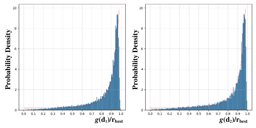
Figure 4: The distribution of decision boundaries $g(\bm{d_{1}})\text{ and }g(\bm{d_{2}})$

Table 4: Comparison of ADBA, ADBA-md, and RayS on MNIST and CIFAR-10 dataset

Datasets	CIFAR-10	MNIST
Attacks
RayS	813.3	697.4
	(364)	(219)
	99.8%	97.0%
ADBA	607.2	600.6
	(216)	(192)
	99.5%	95.3%
ADBA-md	482.3	504.6
	(192)	(166)
	99.9%	97.0%

Appendix E Generality and transferability of ADBA-md

In Subsection 3.2.2, ADBA-md uses $\rho(r)$ to optimize ADB. In Appendix D, the parameters for estimating $\rho(r)$ are determined by analyzing the decision boundaries of many different perturbation directions obtained on the ResNet50 model using the ImageNet dataset.

Despite of the efforts spent in estimating $\rho(r)$, we found empirically that the effectiveness of using $\rho(r)$ is not sensitive to the estimation parameters. Hence, the practical use of ADBA-md is not limited to the ResNet50 model and the ImageNet dataset. ADBA-md can be directly applied to other datasets and models without re-estimating $\rho(r)$.

In this appendix, we design additional experiments to demonstrate the general applicability of ADBA-md without re-estimating $\rho(r)$. Particularly, we randomly select 1000 images from the CIFAR-10 dataset [18] and attack a pre-trained 7-layer CNN model as mentioned in [5] based on the selected images. Additionally, on the MNIST dataset [19], we randomly select 1000 images and attack a pre-trained 7-layer CNNs studied in [5]. We set the perturbation strength threshold $\epsilon=0.031$ for CIFAR-10 and $\epsilon=0.15$ for MNIST. The query budget is set to 10000 for both models. The estimation parameters in the distribution function $\rho(r)=\frac{a}{(|-r/r_{\text{best}}+d|)^{b}+c}$, $r\in[0,r_{\text{best}}]$ are set to be $a=0.0313$, $b=3.066$, $c=0.168$, and $d=1.134$ according to Appendix D. Meanwhile, the search tolerance $\tau$ is set to be 0.002.

Table 4 shows the attack success rate and the average (median) number of queries achieved by ADBA, ADBA-md, and RayS. Our results clearly indicate that, ADBA-md still maintains the highest attack success rate and the lowest number of queries (on average and in median). This confirms that the distribution function $\rho(r)$ in ADBA-md is not sensitive to its estimation parameters. ADBA-md can be easily applied to a variety of target models and datasets without re-estimating $\rho(r)$.

References

- [1] Yang Bai, Yisen Wang and Yuyuan Zeng “Query efficient black-box adversarial attack on deep neural networks” Publisher: Elsevier In Pattern Recognition 133, 2023, pp. 109037
- [2] Wieland Brendel, Jonas Rauber and Matthias Bethge “Decision-Based Adversarial Attacks: Reliable Attacks Against Black-Box Machine Learning Models” arXiv:1712.04248 [cs, stat] arXiv, 2018
- [3] Thomas Brunner, Frederik Diehl, Michael Truong Le and Alois Knoll “Guessing smart: Biased sampling for efficient black-box adversarial attacks” In Proceedings of the IEEE/CVF International Conference on Computer Vision, 2019, pp. 4958–4966
- [4] Jianbo Chen, Michael I. Jordan and Martin J. Wainwright “Hopskipjumpattack: A query-efficient decision-based attack” In 2020 ieee symposium on security and privacy (sp) IEEE, 2020, pp. 1277–1294
- [5] Jinghui Chen and Quanquan Gu “RayS: A Ray Searching Method for Hard-label Adversarial Attack” In Proceedings of the 26th ACM SIGKDD International Conference on Knowledge Discovery & Data Mining Virtual Event CA USA: ACM, 2020, pp. 1739–1747
- [6] Jinghui Chen, Dongruo Zhou, Jinfeng Yi and Quanquan Gu “A frank-wolfe framework for efficient and effective adversarial attacks” Issue: 04 In Proceedings of the AAAI conference on artificial intelligence 34, 2020, pp. 3486–3494
- [7] Pin-Yu Chen et al. “ZOO: Zeroth Order Optimization Based Black-box Attacks to Deep Neural Networks without Training Substitute Models” In Proceedings of the 10th ACM Workshop on Artificial Intelligence and Security Dallas Texas USA: ACM, 2017, pp. 15–26
- [8] Minhao Cheng et al. “Query-Efficient Hard-label Black-box Attack: An Optimization-based Approach” In International Conference on Learning Representations, 2018
- [9] Minhao Cheng et al. “Sign-OPT: A Query-Efficient Hard-label Adversarial Attack” arXiv:1909.10773 [cs, stat] arXiv, 2020
- [10] Jia Deng et al. “ImageNet: A large-scale hierarchical image database” ISSN: 1063-6919 In 2009 IEEE Conference on Computer Vision and Pattern Recognition, 2009, pp. 248–255
- [11] Alexey Dosovitskiy et al. “An Image is Worth 16x16 Words: Transformers for Image Recognition at Scale” arXiv:2010.11929 [cs] arXiv, 2021
- [12] Kevin Eykholt et al. “Robust physical-world attacks on deep learning visual classification” In Proceedings of the IEEE conference on computer vision and pattern recognition, 2018, pp. 1625–1634
- [13] Yan Feng et al. “Boosting black-box attack with partially transferred conditional adversarial distribution” In Proceedings of the IEEE/CVF Conference on Computer Vision and Pattern Recognition, 2022, pp. 15095–15104
- [14] Arka Ghosh, Sankha Subhra Mullick and Shounak Datta “A black-box adversarial attack strategy with adjustable sparsity and generalizability for deep image classifiers” Publisher: Elsevier In Pattern Recognition 122, 2022, pp. 108279
- [15] Kaiming He, Xiangyu Zhang, Shaoqing Ren and Jian Sun “Deep residual learning for image recognition” In Proceedings of the IEEE conference on computer vision and pattern recognition, 2016, pp. 770–778
- [16] Gao Huang, Zhuang Liu, Laurens Van Der Maaten and Kilian Q. Weinberger “Densely connected convolutional networks” In Proceedings of the IEEE conference on computer vision and pattern recognition, 2017, pp. 4700–4708
- [17] Andrew Ilyas, Logan Engstrom, Anish Athalye and Jessy Lin “Black-box adversarial attacks with limited queries and information” In International conference on machine learning PMLR, 2018, pp. 2137–2146
- [18] Alex Krizhevsky and Geoffrey Hinton “Learning multiple layers of features from tiny images” Toronto, ON, Canada, 2009
- [19] Yann LeCun, Léon Bottou, Yoshua Bengio and Patrick Haffner “Gradient-based learning applied to document recognition” In Proceedings of the IEEE 86.11 IEEE, 1998, pp. 2278–2324
- [20] Heng Li et al. “Black-box Adversarial Example Attack towards FCG Based Android Malware Detection under Incomplete Feature Information” In 32nd USENIX Security Symposium (USENIX Security 23) Anaheim, CA: USENIX Association, 2023, pp. 1181–1198
- [21] Huichen Li et al. “Qeba: Query-efficient boundary-based blackbox attack” In Proceedings of the IEEE/CVF conference on computer vision and pattern recognition, 2020, pp. 1221–1230
- [22] Jie Li et al. “Aha! adaptive history-driven attack for decision-based black-box models” In Proceedings of the IEEE/CVF International Conference on Computer Vision, 2021, pp. 16168–16177
- [23] Shan Li and Weihong Deng “Deep facial expression recognition: A survey” In IEEE transactions on affective computing 13.3 IEEE, 2020, pp. 1195–1215
- [24] Simin Li et al. “Towards benchmarking and assessing visual naturalness of physical world adversarial attacks” In Proceedings of the IEEE/CVF Conference on Computer Vision and Pattern Recognition, 2023, pp. 12324–12333
- [25] Yanjie Li et al. “Physical-world optical adversarial attacks on 3d face recognition” In Proceedings of the IEEE/CVF Conference on Computer Vision and Pattern Recognition, 2023, pp. 24699–24708
- [26] Chenhao Lin et al. “Sensitive region-aware black-box adversarial attacks” In Information Sciences 637, 2023, pp. 118929
- [27] Yujia Liu, Seyed-Mohsen Moosavi-Dezfooli and Pascal Frossard “A geometry-inspired decision-based attack” In Proceedings of the IEEE/CVF International Conference on Computer Vision, 2019, pp. 4890–4898
- [28] Teng Long, Qi Gao, Lili Xu and Zhangbing Zhou “A survey on adversarial attacks in computer vision: Taxonomy, visualization and future directions” In Computers & Security 121, 2022, pp. 102847
- [29] Thibault Maho, Teddy Furon and Erwan Le Merrer “Surfree: a fast surrogate-free black-box attack” In Proceedings of the IEEE/CVF Conference on Computer Vision and Pattern Recognition, 2021, pp. 10430–10439
- [30] Seungyong Moon, Gaon An and Hyun Oh Song “Parsimonious black-box adversarial attacks via efficient combinatorial optimization” In International conference on machine learning PMLR, 2019, pp. 4636–4645
- [31] Tianyu Pang et al. “Improving Adversarial Robustness via Promoting Ensemble Diversity” In Proceedings of the 36th International Conference on Machine Learning 97, Proceedings of Machine Learning Research PMLR, 2019, pp. 4970–4979
- [32] Ali Rahmati, Seyed-Mohsen Moosavi-Dezfooli, Pascal Frossard and Huaiyu Dai “Geoda: a geometric framework for black-box adversarial attacks” In Proceedings of the IEEE/CVF conference on computer vision and pattern recognition, 2020, pp. 8446–8455
- [33] Md Farhamdur Reza, Ali Rahmati, Tianfu Wu and Huaiyu Dai “CGBA: Curvature-aware geometric black-box attack” In Proceedings of the IEEE/CVF International Conference on Computer Vision, 2023, pp. 124–133
- [34] Vikash Sehwag et al. “Analyzing the robustness of open-world machine learning” In Proceedings of the 12th ACM Workshop on Artificial Intelligence and Security, 2019, pp. 105–116
- [35] Yucheng Shi, Yahong Han, Yu-an Tan and Xiaohui Kuang “Decision-based black-box attack against vision transformers via patch-wise adversarial removal” In Advances in Neural Information Processing Systems 35, 2022, pp. 12921–12933
- [36] K. Simonyan and A. Zisserman “Very deep convolutional networks for large-scale image recognition” Publisher: Computational and Biological Learning Society In 3rd International Conference on Learning Representations (ICLR 2015), 2015
- [37] Christian Szegedy et al. “Rethinking the inception architecture for computer vision” In Proceedings of the IEEE conference on computer vision and pattern recognition, 2016, pp. 2818–2826
- [38] Mingxing Tan and Quoc Le “EfficientNet: Rethinking Model Scaling for Convolutional Neural Networks” ISSN: 2640-3498 In Proceedings of the 36th International Conference on Machine Learning PMLR, 2019, pp. 6105–6114
- [39] Ningfei Wang et al. “Does Physical Adversarial Example Really Matter to Autonomous Driving? Towards System-Level Effect of Adversarial Object Evasion Attack” In Proceedings of the IEEE/CVF International Conference on Computer Vision (ICCV), 2023, pp. 4412–4423
- [40] Ningfei Wang et al. “Poster: On the system-level effectiveness of physical object-hiding adversarial attack in autonomous driving” In Proceedings of the 2022 ACM SIGSAC Conference on Computer and Communications Security, 2022, pp. 3479–3481
- [41] Xiaosen Wang and Kun He “Enhancing the Transferability of Adversarial Attacks Through Variance Tuning”, 2021, pp. 1924–1933
- [42] Xiaosen Wang et al. “Triangle Attack: A Query-Efficient Decision-Based Adversarial Attack” Series Title: Lecture Notes in Computer Science In Computer Vision – ECCV 2022 13665 Cham: Springer Nature Switzerland, 2022, pp. 156–174
- [43] Cihang Xie et al. “Adversarial examples for semantic segmentation and object detection” In Proceedings of the IEEE international conference on computer vision, 2017, pp. 1369–1378
- [44] Cihang Xie et al. “Feature denoising for improving adversarial robustness” In Proceedings of the IEEE/CVF conference on computer vision and pattern recognition, 2019, pp. 501–509