CWR sequence of invariants of alternating links
and its properties
Abstract.
We present the invariant, a new invariant for alternating links, which builds upon and generalizes the invariant. The invariant is an array of two-variable polynomials that provides a stronger invariant compared to the invariant. We compare the strength of our invariant with the classical HOMFLYPT, Kauffman -variable, and Kauffman -variable polynomials on specific knot examples. Additionally, we derive general recursive ”skein” relations, and also specific formulas for the initial components of the invariant using weighted adjacency matrices of modified Tait graphs.
Key words and phrases:
knot invariant, link invariant, alternating knot, CWR invariant, knots tabulation2020 Mathematics Subject Classification:
57K10 (primary), 57K14 (secondary)1. Introduction
The paper concerns embeddings of a circle in three-dimensional space, known as a knot (or link it there can be more than one component). A significant aspect of knot theory is the development and application of knot invariants, mathematical constructs that distinguish different knots. Among these invariants, polynomial invariants have played a pivotal role. Notable examples include the Alexander polynomial, the Jones polynomial, and the HOMFLYPT polynomial. These invariants have been instrumental in classifying knots and links, particularly alternating links, which are links with diagrams where over-crossings and under-crossings alternate as one travels along each component.
In this paper, we introduce a new invariant for alternating links called the invariant. This invariant is a sequence of two-variable polynomials that generalizes the previously defined invariant. The invariant, while useful, has limitations in its ability to distinguish between certain knots. Our new invariant overcomes these limitations by incorporating additional structural information from the knot’s diagram.
In this paper, Section 2 contains necessary definitions and an example of calculations, and we give proof of invariance of flype-move, needed to apply the proven Tait’s Flype Conjecture. In Section 3 we show that can distinguish between knots that other well-known invariants, such as HOMFLYPT and Kauffman polynomials, cannot. We then give properties of the invariant concerning: connected sum operation, chirality, and mutation. Additionally, we show that the and invariants can be computed using weighted adjacency matrices of modified Tait graphs, providing a practical computational method. Section 4 contains a recursive relation for for diagrams satisfying given conditions. In Section 5 of this paper, we show computationally generated tables of the invariant for prime knots up to eight crossings.
2. Definitions
An diagram of a (non-trivial) knot or link is a generic projection of the knot or link in the plane, a regular -valent graph, with extra information at each vertex indicating which arc of the link pass over the other. Moreover it is alternating when traveling around each link component on a diagram we pass crossing in alternate type fashion (i.e. if one passes an over/under-crossing, the next crossing will be an under/over-crossing, see [15] for a recent survey).
A knot or link diagram is a reduced diagram if a diagram without nugatory crossings, i.e a crossing, such that its neighborhood looks like in Figure 1 left, that can be removed without changing the knot type, and it cannot be separated by any circle in the plane of projection (i.e. the diagram as projection has one connected component).
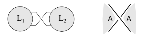
By a region of a reduced diagram we mean a face of the underlying projection of the link. The diagram can be checkerboard-shaded so that every edge separates a shaded region (black region) from an unshaded one (white region).
Moreover, we can assume [11, 15] that if the diagram is reduced then any region of type as shown in Figure 1 right is a black region, otherwise it is a white region. Therefore, from now on, we can always assume this convention of coloring of diagram regions, when the diagram is reduced and alternating.
We consider two associated with graphs (also known as Tait graphs) the shaded checkerboard graph and the unshaded checkerboard graph . The graph has vertices corresponding to the black region regions of , and an edge between two vertices for every crossing at which the corresponding regions meet. The dual graph is defined by analogy but the vertices correspond to the white regions.
On each edge of graph and we assign its weight as a variable when the corresponding crossing was positive and variable if it was negative crossing.
An unoriented graph is then obtained from an unoriented graph by consolidating all multiple edges between the same pair of vertices to a single edge that has its weight equal to the product of weights all edges being consolidated. The same goes with defining graph from .
For , we define as a two-variable polynomial where the sum is taken over all unoriented cycles (i.e. simple closed paths) in a graph of the diagram and the product is taken over all edges in a given cycle.
We define as a sum where the sum is taken over all edges in (when there are no edges in case of the trivial knot we can put the value as ).
By analogy we define for all considering a graph
instead of . For an integer , we define as an ordered tuple
, when there are no cycles of length in a given graph we put the corresponding value as . Define of an alternating knot or link as a sequence of invariants (ordered tuple):
of any reduced alternating diagram of . When for every , for some integer then we omit those values in the sequence for , therefore the sequence is finite as there are finitely many cycles in a finite graph.
2.1. An example
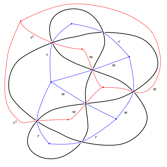
For the knot we have calculations show in Figure 2, that is .
2.2. An invariance
Theorem 2.1.
For any pair and of reduced alternating diagrams of a given alternating link, we have
Proof.
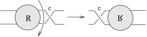
We use the theorem known as Tait’s Flype Conjecture, which states that if and are reduced alternating diagrams, then can be obtained from by a sequence of flype-moves (a local move on a knot diagram that involves flipping a part of the diagram, see Figure 3) if and only if and represent the same link. This conjecture has been proven true by Menasco and Thistlethwaite [13, 14].
The diagrams can be checkerboard-colored, resulting in two types of regions (black and white). Let us fix the reduced alternating diagram before the flype as and after the flype as . We can now fix the graph as one of or for a diagram and the graph as the corresponding graph for a diagram . First, we notice that the black and white corresponding regions before and after the flype-move preserves their color. Second, we notice that the flype-move preserves the length of any corresponding cycles in graphs and , and also preserves the number of consolidated edges crossings and their weights.
Therefore, for in (and respectively) there is a one-to-one correspondence between cycle summands in the definition of the functions. The rest of the proof is in the spirit of the proof of invariants of our previous (weaker) invariant (see [5]). Namely, it is sufficient to prove that the corresponding cycles preserve the product of the weights of all their edges (that forms the cycle).
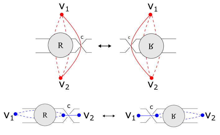
This can be seen in the general situation in Figure 4 for the cases of black or white graphs and we are considering, that only the relative position of edges can vary between corresponding cycles so the product is preserved (as a commutative operation). We can easily conclude that if any cycle from does not go through both and then there is a one-to-one correspondence between cycles in and cycles in and each corresponding cycle preserves its number of edges and their weights. It is because the cycles are either outside the shown flype tangle (so they do not change) or they are completely inside a tangle (plus eventually touching the unlabeled dot in the figure).
When a cycle in passes through both and then there is a corresponding cycle in that in Case I: preserves its number, its order, and their weight of edges involved in the cycle, in Case II: for all edges between and , the weights are preserved but the order may vary so this does not change the product od weights in the cycle.
∎
3. Properties
Let us consider the classical alternating knots and non-split link polynomial invariants: HOMFLYPT [4, 17], Kauffman -variable [7, 10] and Kauffman -variable [8] polynomials, and call them here: HOMFLYPT, Kauffman3v and Kauffman2v respectively.
Examples, were HOMFLYPT, Kauffman3v, and Kauffman2v invariants, which are non-comparable in general are shown in Figure 5. An arrow means that the invariant distinguishes the knots indicated in the arrow label and does not. The letter after a knot name stands for the mirror image of that knot. There are examples (shown in Figure 5) where invariant is stronger than the mentioned other three invariants. But we cannot find examples when is strictly weaker, we computationally done a search in the knot tables of knots up to crossings, including their mirror images. Examples in the labels were found using [1, 2, 3].
In addition, we find that for a knotted pair and are indistinguishable by HOMFLYPT, Kauffman3v, Kauffman2v, signature, unknotting number, bridge index, -genus, Khovanov and Knot Floer homologies [1, 2, 3] (see [12] for a few other invariants that do not tell this knots apart). To distinguish we can use our invariant, we have:
, and
3.1. Generalization of the other invariants
With our definition, invariant generalize the invariant defined in one of our previous papers [5] as follows:
where the curly brackets mean taking the ordered tuple to an unordered tuple, and the sum of tuples is performed as the sum of corresponding coordinates in the tuples.
invariant is strictly stronger than , for example, the pair and cannot be distinguished by as shown in [5] (together with their diagrams and resulting graphs), but tell them apart, because:
, and
From invariant, we can naturally read the crossing number and , we have the following.
Proposition 3.1.
For any alternating non-split link
Proof.
The alternating knot (or link) invariants , , and can be calculated from the link reduced alternating diagram ([6, 16, 19, 20]). In that kind of diagram, we can simply count each crossing as the sum of powers in the formula for or expressed as a sum of unimodal monomials, where each monomial is a one-variable function, because otherwise it would not be reduced alternating diagram as it can be reduced by a Reidemeister II move after possibly a flype-move. ∎
It is also useful in increasing efficiency when searching for different knots with the same invariant as they must have the same crossing number (and there are finitely many such knots).
When counting the product of weights for the cycle contribution in the formula for , the sum of powers of and in each monomial cannot be greater than as this is the total number of edges in a considered graph (counting with multiplications for the consolidate edges).
3.2. Connected sum
is additive concerning the connected sum, we have the following.
Theorem 3.2.
If and are alternating knots, or non-split links, then
where the sum of tuples is performed as the sum of corresponding coordinates in the tuples.
Proof.
Let denote a graph obtained from graphs and by gluing them along one vertex (identification of one arbitrarily chosen vertex from each graph). This operation in this context of graphs is also called block sum. It can be straightforwardly examined that the connected sum operation can have the reduced alternating projection such that it merges exactly one black region and one white region from each checkerboard coloring of complementary regions of reduced alternating diagrams for and . From this operation we get that and . Moreover, in the resulting graphs, no two edges merge and no edge is canceled. There are no new cycles besides the ones completely embedded in graphs for and because each new closed path passing through the joining vertex must pass it twice (otherwise it is one of the old cycles) and that contradicts the assumption that the path is simple. Therefore the cycles as a set just adds in counting , causing ∎
3.3. Non-mutant knots
Mutant knots are the knots such that they have diagrams that differ only by a (Conway’s) mutation operation. The mutation operation modifies a knot by first cutting, then rotating (by ) and finally gluing arcs to preserve the number of components (that is one component in our knot case), the operation is performed in a -tangle along a –sphere embedded in and intersecting transversely the knot in exactly four points.
Our computations show that the invariant is strong enough to distinguish all non-mutant knots in the tables with up to crossings, including their mirror images (when the knot is chiral). An example of a non-mutant pair (see [18]) that the invariant does not distinguish is and , shown in Figure 7. The invariant in their case is equal to
3.4. Chirality
We have the straightforward formula for the invariant for the mirror image of a given link knowing the value for the original link.
Proposition 3.3.
For any alternating link , if we express as
, then we have
, where is the mirror
image of .
Proof.
Let be a reduced alternating diagram for obtained by switching crossing types of every crossing in a given reduced alternating diagram for . Therefore, the diagrams and have corresponding regions in the projection complement but with switched colors, therefore the black and white graphs are exchanged. All cycles geometrically stay unchanged and the weights of each edge in a cycle are also switched, replacing variable with and vice versa because switching crossing types changes the sign of a crossing to the opposite. ∎
In the set of alternating prime knots up to crossings, the can tell apart a knot and its mirror image if it is chiral (see [18]). This is in contrast to invariants HOMFLYPT, Kauffman3v, and Kauffman2v which cannot distinguish between the knot from its mirror image.
The knot is not equivalent to its mirror image, but
.
3.5. Matrix formulae for and
The weighted adjacency matrix of a (simple) graph without loops, is the symmetric matrix whose rows and columns are indexed by some consistent orderings of vertices such that if vertices and are endpoints of an edge in and otherwise. Define also the adjacency matrix as a weighted adjacency matrix where all edge weights are equal to .
Proposition 3.4.
Let (resp. ) be the weighted adjacency matrices for a graph (resp. ) of an alternating link , and (resp. ) their corresponding adjacency matrices respectively.
Proof.
It follows from a standard Graph Theory argument, see for example [9, Theorem 2.5.6]. Counting the number of closed directed paths of length and in a graph equal and respectively for a standard adjacency matrix of a graph . We need only to consider weights. In case we count paths of length from each vertex to itself, so counting one edge with weight from and one with weight back to be consistent with the definition of multiplication of this to weights equal just single weight. In the case of , we count only simple paths (cycles) of length that are multiplied when forming a cycle invariant and added when summing all cycles in our invariant , which is consistent with matrix multiplications in this context. The denominator here is because we consider unoriented graphs so the closed path in one direction is the same as the path in the opposite direction. ∎
Example 3.5.
Let us calculate with the above method and invariants for knot from its diagram shown in Figure 2.
We have for the graphs and in this figure that ,
,
,
,
,
,
therefore and
4. Recursive relations
For an integer , let the alternating reduced non-split links , , , and differ only locally by changing tangles as shown in Figure 8. We can derive the following recursive ”skein” relations for , with the restrictions on diagrams.

Theorem 4.1.
Assume that all diagrams used in the following relations are reduced, alternating, and non-split. Then, we have for all integers :
-
(1)
-
(2)
Proof.
The proof goes by counting an invariant while taking care of the cases where the concerning cycles pass through given tangles shown in Figure 8.
Let us consider the first equation. The left-hand side is calculated with all cycles of length , the right-hand side is calculated considering cycles of length not passing through that is (from the assumption that and is reduced) and those cycles of length that passes through correspond one-to-one with the cycles that pass through , because we have only one edge in passing through from the assumption that and is reduced. The weights of edges, that are considered in counting , change with the appropriate accumulated weigh scale by . Similar arguments are for the second equation, from the assumption that and are reduced diagrams. ∎
5. Values for knots in tables
We computationally generate, the following Table LABEL:table1 of the invariant of knots.
| DT | Rolf | invariant |
|---|---|---|
We use our code, written in SageMath [3]. In this paper, there are the values for prime knots up to the crossing number equal to . The values of the invariant for knots in the knot tables up to crossings can be found in the CWRknots folder in https://drive.google.com/drive/folders/1mdF8zHY9Avmy1GnY4co3neH7q7b2Vnso.
References
- [1] D. Bar-Natan. The Mathematica Package KnotTheory, Available at https://katlas.org/wiki/Main_Page (27/05/2024)
- [2] M. Culler, N.M. Dunfield, M. Goerner and J.R. Weeks, SnapPy, a computer program for studying the geometry and topology of -manifolds, Available at http://snappy.computop.org (27/05/2024)
-
[3]
Developers, The Sage, Sagemath, the Sage Mathematics Software System (Version 10.1), (2023),
https://www.sagemath.org - [4] P. Freyd, D. Yetter, J. Hoste, W. B. R. Lickorish, K. Millett and A. Ocneanu, A new polynomial invariant of knots and links, Bull. AMS 12 (1985), 239–-246.
- [5] M. Jabłonowski, A polynomial pair invariant of alternating knots and links, (2024), preprint https://arxiv.org/abs/2307.08516
- [6] L.H. Kauffman, New invariants in the theory of knots, Amer. Math. Monthly 95 (1988), 195–242.
- [7] L.H. Kauffman, A Tutte polynomial for signed graphs, Discrete Applied Mathematics 25 (1989), 105–127.
- [8] L.H. Kauffman, An invariant of regular isotopy, Transactions of the AMS 318 (1990), 417-–471.
- [9] U. Knauer and K. Knauer, Algebraic graph theory. Morphisms, Monoids and Matrices, Vol.41 De Gruyter Studies in Mathematics, Walter de Gruyter GmbH, (2019).
- [10] K. Lafferty, The three-variable bracket polynomial for reduced, alternating links, Rose-Hulman Undergraduate Mathematics Journal 14 (2013), 98–-113.
- [11] J.B. Listing, Vorstudien zur Topologie, Gottinger Studien(Abtheilung 1) 1 (1847), 811–875.
-
[12]
C. Livingston and A.H. Moore, KnotInfo: Table of Knot Invariants,
https://knotinfo.math.indiana.edu/, (June 2024). - [13] W. Menasco and M.B. Thistlethwaite, The Tait flyping conjecture, Bull. Amer. Math. Soc. (1991), 403–412.
- [14] W. Menasco and M.B. Thistlethwaite, The classification of alternating links, Annals of Mathematics (1993), 113–171.
- [15] W. Menasco, Alternating Knots, In Encyclopedia knot theory, CRC Press (2021) 167–178.
- [16] K. Murasugi, Jones polynomials and classical conjectures in knot theory, Topology 26.2 (1987), 187–194.
- [17] J. Przytycki and P. Traczyk, Invariants of links of the Conway type, Kobe J. Math. 4 (1988), 115–-139.
- [18] A. Stoimenow, Knot data tables, Available at https://stoimenov.net/stoimeno/homepage/ptab/index.html (27/05/2024)
- [19] M.B. Thistlethwaite, A spanning tree expansion of the Jones polynomial, Topology 26 (1987), 297–-309
- [20] M.B. Thistlethwaite, Kauffman’s polynomial and alternating links, Topology 27 (1988), 311–318.