\UseRawInputEncoding

Hybrid Beamforming Design for RSMA-assisted mmWave Integrated Sensing and Communications

Jun Gong, Student Member, IEEE, Wenchi Cheng, Senior Member, IEEE, Jiangzhou Wang, Fellow, IEEE,
and Jingqing Wang, Member, IEEE
Jun Gong, Wenchi Cheng, and Jingqing Wang are with the State Key Laboratory of Integrated Services Networks, Xidian University, Xi’an, 710071, China (e-mails: jungong@stu.xidian.edu.cn, wccheng@xidian.edu.cn, jqwangxd@xidian.edu.cn). Jiangzhou Wang is with the School of Engineering, University of Kent, Canterbury CT2 7NT, U.K. (e-mail: j.z.wang@kent.ac.uk).
Abstract

Integrated sensing and communications (ISAC) has been considered one of the new paradigms for sixth-generation (6G) wireless networks. In the millimeter-wave (mmWave) ISAC system, hybrid beamforming (HBF) is considered an emerging technology to exploit the limited number of radio frequency (RF) chains in order to reduce the system hardware cost and power consumption. However, the HBF structure reduces the spatial degrees of freedom for the ISAC system, which further leads to increased interference between multiple users and between users and radar sensing. To solve the above problem, rate split multiple access (RSMA), which is a flexible and robust interference management strategy, is considered. We investigate the joint common rate allocation and HBF design problem for the HBF-based RSMA-assisted mmWave ISAC scheme. We propose the penalty dual decomposition (PDD) method coupled with the weighted mean squared error (WMMSE) minimization method to solve this high-dimensional non-convex problem, which converges to the Karush-Kuhn-Tucker (KKT) point of the original problem. Then, we extend the proposed algorithm to the HBF design based on finite-resolution phase shifters (PSs) to further improve the energy efficiency of the system. Simulation results demonstrate the effectiveness of the proposed algorithm and show that the RSMA-ISAC scheme outperforms other benchmark schemes.

Index Terms:
Integrated sensing and communications, rate-splitting multiple access, hybrid beamforming, millimeter wave.

I Introduction

The sixth generation (6G) of wireless networks is regarded as a major enabler for emerging services such as autonomous driving, smart manufacturing, remote health care, and digital twins [1]. The aforementioned applications require networks with both high-throughput communication and high-accuracy sensing capabilities. Meanwhile, the exponential growth of wireless services and the massive number of connections to wireless devices are straining spectrum resources, which will create an urgent need for additional spectrum, of which the radar frequency bands are one of the best candidates for coexistence with communication systems [2]. Based on the above service and spectrum coexistence requirements, integrated sensing and communications (ISAC) technology has arisen and attracted extensive resesarch attention in industry and academia [3]. Recently, the international telecommunication union (ITU) has released the 6G overall objective recommendation, in which ISAC, as one of the six key scenarios, aims to enable ubiquitous wireless sensing capabilities for 6G network infrastructures [4].

Distinguished from communication and radar coexistence designs [5],[6], ISAC is designed to simultaneously realize communication and sensing functions by sharing wireless resources, hardware platforms, and joint signal processing frameworks, yielding integration gains and collaboration gains to the system. Specifically, ISAC signal design methods can be classified into three categories: sensing-centric design (SCD), communication-centric design (CCD), and joint design (JD). Early SCD scheme modulates the communication symbols into the radar chirp signals [7]. The CCD scheme is mainly based on orthogonal frequency division multiplexing (OFDM) waveforms to design the ISAC signal [8], [9]. However, the JD scheme does not rely on the existing waveforms and designs the ISAC waveforms from scratch in order to improve the freedom and flexibility of the system. The authors of [10] pioneered a JD approach based on optimization techniques to solve the problem of designing the constant envelope waveforms for the ISAC system. In addition, since multiple-input multiple-output (MIMO) technology can further improve the diversity gain and degrees of freedom (DoFs) of the system, the integration design of MIMO communication and MIMO radar in the spatial domain is an inevitable trend. The authors of [11] proposed a scheme that utilizes the sidelobe level of the MIMO radar beampattern to represent the communication symbols, while the main beam is only used for target sensing. Further, the beamforming design of the MIMO-ISAC system can be formulated as nonlinear optimization problems considering communication performance metrics (e.g., throughput [12], [13], symbol error rate (SER) [14], singal-to-interference-plus-noise ratio (SINR) [15], etc.) and sensing performance metrics (e.g., beampattern matching mean-square error [16],[17], signal-to-clutter-plus-noise ratio (SCNR) [18], Cramér-Rao bound (CRB) [19], [20], etc.).

All of the above ISAC research is based on the sub-6 GHz band, but in order to cope with the explosive growth of wireless devices and services, the millimeter-wave (mmWave) spectrum band of 30-300 GHz can further dramatically improve communication capacity and target sensing accuracy, and thus, become a new research spectrum band for ISAC. The authors of [21] achieved gigabit communication rates and centimeter-level sensing accuracy for short distances based on the IEEE 802.11ad protocol at 60 GHz carriers. However, the short wavelength of mmWave leads to severe road loss and rain fading [22]. Therefore, transmitters usually need to employ massive MIMO (mMIMO) technology to form high beam gains to overcome these drawbacks. Note that the fully digital large-scale antenna array structure, i.e., each antenna needs to be equipped with a radio frequency (RF) chain, will lead to high hardware costs and power consumption. To address the above issues, the mmWave communication base station (BS) has widely adopted hybrid beamforming (HBF) architectures [23],[24],[25], which require only a few RF chains to be connected to the large-scale antenna arrays via phase shifters (PSs), thus reducing the hardware cost and improving the energy efficiency of the system. In addition, the above hybrid architecture was also demonstrated in phased-MIMO radar [26], which integrates the advantages of the diversity gain of orthogonal waveforms of MIMO radar and the high beam gain of phased-array radar to improve the SCNR of the received signals and the target detection probability. Based on the similarities between communication hybrid architectures and phased-MIMO radars, the research of HBF has been in mmWave ISAC systems. The authors of [27] have pioneered the HBF design for ISAC systems that minimizes the weighted sum of the radar beampattern error and the communication precoding error. The complete uplink and downlink communication protocols and target sensing steps in HBF-based mmWave ISAC systems were given in [28]. The authors of [29],[30] presented the HBF design scheme based on the alternating direction method of multipliers (ADMM) algorithm.

In the MIMO-ISAC systems mentioned above, spatial division multiple access (SDMA) was used to manage the interference between the user and the radar. However, rate-splitting multiple access (RSMA) is a non-orthogonal transmission strategy based on rate-splitting (RS) precoding at the transmitter and successive interference cancellation (SIC) decoding at the receiver, which provides strong anti-interference capability for multi-antenna wireless networks [31]. Specifically, RSMA divides user messages into common and private parts, encodes the common part jointly into common data streams decoded by SIC for multiple users, and encodes the private part independently into private data streams decoded by corresponding users. RSMA reconciles two extreme interference management strategies, SDMA, which treats interference entirely as noise, and non-orthogonal multiple access (NOMA), which decodes interference completely, to achieve higher spectral and energy efficiencies [32],[33]. Further, the authors of [34],[35] proposed a scheme for the RSMA-assisted ISAC system and demonstrated the advantages of RSMA in managing interference between communication users and interference between dual functions. The authors of [36] investigated RSMA-assisted multi-BS cooperative ISAC systems for advanced interference management and high-accuracy localization services.

Motivated by the advantages of mmWave hybrid architecture‘s low power consumption and robust RSMA interference management, we introduce RSMA in mmWave ISAC systems to address the joint common rate allocation and HBF design issues in order to fill the research gap in this area. We further improve the performance trade-off region of the ISAC system and reveal the mechanism of the RSMA strategy common data streams at the dual functions of communication and sensing. The main contributions of this paper are summarized as follows:

  • 1)

    We first propose mmWave ISAC system with HBF structure assisted by RSMA. We formulate the weighted sum rate (WSR) maximization problem by joint common rate allocation and HBF design, subject to the constraints of target sensing SCNR threshold, PSs unit-modulus, the total power budget, and the necessity for accurate correct decoding of common messages.

  • 2)

    The penalty dual decomposition (PDD) method coupled with the weighted mean squared error minimization (WMMSE) method is proposed to solve the above high-dimensional non-convex problem. First, the WMMSE method is used to transform the original problem into an equivalent form that is easy to solve. Next, the PDD algorithm of [37],[38] is used to solve the corresponding problem by means of an inner and outer double loop, in which the variables are updated in the form of a closed-form solution in the inner loop. Rigorous proof of the algorithm’s converges to the Karush-Kuhn-Tucker (KKT) point of the original optimization problem is provided.

  • 3)

    We extend the proposed algorithm to the HBF design based on finite-resolution PSs, which further reduces the hardware cost and power consumption and improves the energy efficiency of the system.

  • 4)

    Our simulation results show that the proposed WMMSE-PDD algorithm converges quickly. For both high and low spatial correlation channels, the RSMA-ISAC scheme outperforms the SDMA-ISAC and NOMA-ISAC schemes in terms of WSR and anti-clutter interference capability. We reveal that the common data stream has a dual function in mitigating multi-user interference and trade-offs between communication and sensing performance.

The remainder of this paper is organized as follows. In Section II, we introduce the HBF-based RSMA-assisted mmWave ISAC system model and problem formulation. The specific algorithm for solving the optimization problem is presented in Section III. Section IV presents the extension of the algorithm to ISAC systems with finite resolution PSs. The simulation results are presented in Section V. Finally, our conclusions are provided in Section VI.

Notations: Upper-case and lower-case boldface letters denote matrices and vectors, respectively. $(\cdot)^{*}$, $(\cdot)^{T}$, $(\cdot)^{H}$, $(\cdot)^{-1}$, and $(\cdot)^{\dagger}$ denote complex conjugate, transpose, Hermitian transpose, matrix inversion, and Moore-Penrose matrix inversion, respectively. $\operatorname{tr}(\cdot)$, $\left\|\cdot\right\|_{p}$, and $\Re\{\cdot\}$ denote the trace of the matrix, $l_{p}$ norm operation, and the real part of a complex variable, respectively. $\mathbb{E}\{\cdot\}$ denotes the expectation. $\mathbb{C}^{m\times n}$ denotes the space of $m\times n$ complex matrices. $\left|\boldsymbol{\rm A}(m,n)\right|$ denotes the modulus of the element in the $m$-th row and $n$-th column of matrix A. ${\rm vec\{\cdot\}}$ denotes the matrix vectorization. ${\rm diag}\{\boldsymbol{\rm c}\}$ denotes the diagonal matrix, whose diagonal elements are formed by the vector $\boldsymbol{\rm c}$. $\otimes$ denotes the Kronecker products between two matrices.

Refer to caption
Figure 1: RSMA-assisted mmWave ISAC system.

II System Model and Problem Formulation

In this section, we first introduce the RSMA-assisted mmWave ISAC system model, the performance metrics of the communication, and sensing functions, and then formulate the HBF problem.

II-A Transmit Model

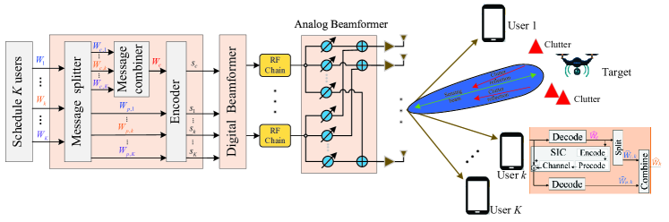
Consider an RSMA-assisted mmWave ISAC system as shown in Fig. 1, where one BS with $N_{t}$ transmit antennas and $N_{r}$ receive antennas simultaneously serve $K$ single-antenna downlink user communications while engaging in radar target detection. Let $\mathcal{K}=\{1,2,\cdots,K\}$ represent the set of all user indexes. Specifically, the messages of $K$ users are first split and encoded to form $K+1$ data streams via the RSMA technique. Further, to reduce the hardware cost and complexity, we use an HBF structure to transmit the data stream, which is first digitally processed at the baseband using a digital beamformer, and then the digitally processed signal is upconverted to the carrier frequency through the RF chains, followed by PSs to implement an analog beamformer. Without loss of generality, it is assumed that the multiple antennas are uniform linear arrays (ULA) and the number of RF chains is ${N}_{\rm RF}$ with the constraint $K+1\leq{N}_{\rm RF}\leq N_{t}$. Since a monostatic sensing model is considered, the transmitter operates in time-division duplex (TDD) mode to avoid interference between the transmit and sensing echo signals.

According to [31], when we consider the RSMA transmission scheme, the message $W_{k}$ of the $k$-th user is first split into two parts, one of which is the common part $W_{c,k}$, and the other is the private part $W_{p,k}$, $\forall k\in\mathcal{K}$. The common data stream $s_{c}$ is obtained by encoding the common message $W_{c}$ formed by combining all user common parts $\{W_{c,1},\cdots,W_{c,K}\}$, while private data streams $\{s_{1},\cdots,s_{K}\}$ are obtained by encoding the private parts $\{W_{p,1},\cdots,W_{p,K}\}$. Define the vector $\boldsymbol{\rm s}=[s_{c},s_{1},\cdots,s_{K}]^{T}\in\mathbb{C}^{(K+1)\times 1}$ as data streams with unit power and satisfy $\mathbb{E}\{\boldsymbol{\rm s}\boldsymbol{\rm s}^{H}\}=\boldsymbol{\rm I}_{K+1}$. Next, the data stream $\boldsymbol{\rm s}$ undergoes hybrid beamforming to obtain a dual-function integrated signal that simultaneously achieves multi-user communication and radar target detection. Accordingly, the transmit ISAC signal, denoted by $\boldsymbol{\rm x}\in\mathbb{C}^{{N_{t}}\times 1}$, can be expressed as

$\displaystyle\boldsymbol{\rm x}$ $\displaystyle=\boldsymbol{\rm F}_{\rm RF}\boldsymbol{\rm F}_{\rm D}\boldsymbol{\rm s}$ (1)
$\displaystyle=\boldsymbol{\rm F}_{\rm RF}\boldsymbol{\rm f}_{c}s_{c}+\sum_{i\in\mathcal{K}}\boldsymbol{\rm F}_{\rm RF}\boldsymbol{\rm f}_{{\rm D},i}s_{i},$

where $\boldsymbol{\rm F}_{\rm D}=[\boldsymbol{\rm f}_{c},\boldsymbol{\rm f}_{\rm D,1},\cdots,\boldsymbol{\rm f}_{{\rm D},K}]\in\mathbb{C}^{N_{\rm RF}\times(K+1)}$ is the digital beamforming matrix, in which $\boldsymbol{\rm f}_{c}$ is the common data stream precoder and $\boldsymbol{\rm f}_{{\rm D},k},k\in\mathcal{K}$ is the precoder for the $k$-th user’s private data stream. $\boldsymbol{\rm F}_{\rm RF}\in\mathbb{C}^{N_{t}\times N_{\rm RF}}$ is the analog beamforming matrix that is composed of $N_{t}\times N_{\rm RF}$ phase shifters with a fully connected structure [25]. As the phase shifter can only adjust the phase of the signal, all entries in the $\boldsymbol{\rm F}_{\rm RF}$ should satisfy the unit modulus constraints, e.g., $\left|\boldsymbol{\rm F}_{\rm RF}(i,j)\right|=1$.

II-B Communication Model And Metrics

Under the above transmit signal model, the receive signal, denoted by $y_{k}$, at $k$-th single antenna user can be expressed as

$\displaystyle y_{k}$ $\displaystyle=\boldsymbol{\rm h}_{k}^{H}\boldsymbol{\rm x}+n_{k}$ (2)
$\displaystyle=\boldsymbol{\rm h}_{k}^{H}\boldsymbol{\rm F}_{\rm RF}\boldsymbol{\rm f}_{c}s_{c}+\sum_{i\in\mathcal{K}}\boldsymbol{\rm h}_{k}^{H}\boldsymbol{\rm F}_{\rm RF}\boldsymbol{\rm f}_{{\rm D},i}s_{i}+n_{k},$

where ${\boldsymbol{\rm h}}_{k}\in\mathbb{C}^{N_{t}\times 1}$ is the channel vector from the transmitter to the $k$-th user and is assumed to be known by the BS. $n_{k}\sim\mathcal{CN}\left(0,\sigma_{{k}}^{2}\right)$,$k\in\mathcal{K}$, is the additive white Gaussian noise (AWGN) with zero mean and variance $\sigma_{{k}}^{2}$. Due to the sparse scattering environment of mmWave communications, the channel is directional and spatially sparse in the angular domain. Without loss of generality, we adopt the widely used Saleh-Valenzuela channel for mmWave communications [22], so $\boldsymbol{\rm h}_{k}$ can be written as

$\displaystyle\boldsymbol{\rm h}_{k}=\sqrt{\frac{N_{t}}{L_{k}}}\sum_{\ell=1}^{L_{k}}\beta_{\ell,k}\boldsymbol{\rm a}\left(\theta_{\ell,k}\right),$ (3)

where $L_{k}$ denotes the number of paths for the $k$-th user. $\beta_{1,k}$ and $\beta_{\ell,k},(2\leq\ell\leq L_{k})$ denote the complex gains of the $k$-th user line-of-sight (LoS) component and non-line-of-sight (NLoS) components, respectively. $\theta_{\ell,k}\in[-\frac{\pi}{2},\frac{\pi}{2}]$ is the angle of departure (AOD) of the $l$-th path, and the array steering vector $\mathbf{a}(\theta)\in\mathbb{C}^{N_{t}\times 1}$ can be given by

$\displaystyle\mathbf{a}(\theta)=\frac{1}{\sqrt{N_{t}}}\big{[}1,e^{j\frac{2\pi}{\lambda}d\sin(\theta)},\cdots,e^{j\left(N_{t}-1\right)\frac{2\pi}{\lambda}d\sin(\theta)}\big{]}^{T},$ (4)

where $\lambda$ and $d$ are the carrier wavelength and the antenna spacing, respectively. In this paper, we use a half-wavelength antenna array, i.e., $d=\lambda/2$.

According to the decoding criterion of the RSMA scheme [31], each user first decodes the common data stream $s_{c}$ into $\hat{W}_{c}$ by treating the interference from the private data streams $\{s_{1},\cdots,s_{K}\}$ as noise. Thus, the SINR, denoted by $\gamma_{c,k}$, of decoding $s_{c}$ at the $k$-th user is given by

$\displaystyle{\gamma}_{c,k}=\frac{\left|\mathbf{h}_{k}^{H}\mathbf{F}_{\rm RF}\mathbf{f}_{c}\right|^{2}}{\sum\limits_{i\in\mathcal{K}}\left|\mathbf{h}_{k}^{H}\mathbf{F}_{\rm RF}\mathbf{f}_{{\rm D},i}\right|^{2}+\sigma_{{k}}^{2}}.$ (5)

Next, the common data stream reconstructed by $\hat{W}_{c}$ is subtracted from the received signal $y_{k}$ using SIC. Then, user $k$ decodes the private data stream $s_{k}$ into $\hat{W}_{p,k}$ by treating the interference from private data streams $\{s_{i}\},i\neq k$ as noise. The SINR, denoted by $\gamma_{k}$, of decoding $s_{k}$ at the $k$-th user is then given by

$\displaystyle{\gamma}_{k}=\frac{\left|\mathbf{h}_{k}^{H}\mathbf{F}_{\rm RF}\mathbf{f}_{{\rm D},k}\right|^{2}}{\sum\limits_{i\in\mathcal{K},i\neq k}\left|\mathbf{h}_{k}^{H}\mathbf{F}_{\rm RF}\mathbf{f}_{{\rm D},i}\right|^{2}+\sigma_{{k}}^{2}}.$ (6)

Finally, user $k$ splits $\hat{W}_{c,k}$ from the common message $\hat{W}_{c}$ and combines it with $\hat{W}_{p,k}$ to reconstruct the private message $\hat{W}_{k}$. Based on Eqs. (5) and (6), the achievable rates of decoding $s_{c}$ and $s_{k}$ for user $k$ are $R_{c,k}=\log_{2}\left(1+\mathrm{\gamma}_{c,k}\right)$ and $R_{k}=\log_{2}\left(1+\mathrm{\gamma}_{k}\right)$, respectively. To ensure that all users can successfully decode the common message, the rate of the common data stream $s_{c}$ can not exceed $R_{c}={\rm min}\{R_{c,1},\cdots,R_{c,K}\}$. According to the structure of RS, the rate of the common message is divided into $K$ portions, satisfying $\sum_{k\in\mathcal{K}}C_{k}=R_{c}$, where $C_{k}$ is the rate corresponding to the common part $W_{c,k}$ of the $k$-th user message. Thus, the total achievable rate for user $k$ consists of the sum of the rates of the common part $W_{c,k}$ and the private part $W_{p,k}$. In the RSMA-assisted ISAC system, for the communication function, we select the weighted sum rate (WSR), denoted by $R_{\rm WSR}$, as the performance metric of the system, which can be expressed as

$\displaystyle R_{\rm WSR}=\sum_{k\in\mathcal{K}}\alpha_{k}(C_{k}+R_{k}),$ (7)

where $\alpha_{k}$ is the weight factor representing the $k$-th user priority.

II-C Radar Sensing Model And Metrics

In ISAC systems, the radar sensing waveform multiplexes the communication signal $\boldsymbol{\rm x}$. According to [26], we propose the HBF architecture for radar sensing that combines the advantages of the high directional gain of phased-array radars and the diversity gain provided by multiple waveforms of conventional MIMO radars. The purpose of radar sensing is to realize functions such as target detection and parameter estimation in a cluttered environment. In this paper, we assume that the sensing function of the ISAC system is to detect a radar target (located at angles $\theta_{0}$) of interest in the presence of interference from $Q$ clutter located at different angles $\theta_{q},q\in\mathcal{Q}=\{1,\cdots,Q\}$. Thus, the echo signal arriving at the ISAC receiver, denoted by $\boldsymbol{\rm y}_{r}$, can be expressed as

$\displaystyle\boldsymbol{\rm y}_{r}=$ $\displaystyle\underbrace{\sqrt{N_{r}N_{t}}\xi_{0}\boldsymbol{\rm a}_{r}\left(\theta_{0}\right)\boldsymbol{\rm a}_{t}^{H}\left(\theta_{0}\right)\boldsymbol{\rm F}_{\rm RF}\boldsymbol{\rm F}_{\rm D}\boldsymbol{\rm s}}_{\text{target }}+$ (8)
$\displaystyle\underbrace{\sqrt{N_{r}N_{t}}\sum_{q\in\mathcal{Q}}\xi_{q}\boldsymbol{\rm a}_{r}\left(\theta_{q}\right)\boldsymbol{\rm a}_{t}^{H}\left(\theta_{q}\right)\boldsymbol{\rm F}_{\rm RF}\boldsymbol{\rm F}_{\rm D}\boldsymbol{\rm s}}_{\text{clutter }}+\boldsymbol{\rm z}_{r},$

where $\mathbf{a}_{t}(\theta)\in\mathbb{C}^{N_{{t}}\times 1}$ and $\mathbf{a}_{r}(\theta)\in\mathbb{C}^{N_{{r}}\times 1}$ denote the transmit and receive steering vectors, respectively, similar to the definition of Eq.(4). $\mathbf{z}_{r}\sim\mathcal{CN}\left(\mathbf{0}_{N_{r}},\sigma_{{z}}^{2}\mathbf{I}_{N_{r}}\right)$ represents the AWGN with zero mean and variance $\sigma_{{z}}^{2}$. $\xi_{0}$ and $\xi_{q}$ denote the complex fading coefficients of the target and the $q$-th clutter, respectively. Based on the radar equations [39], the modulus of $\xi_{0}$, denoted by $\left|\xi_{0}\right|$, can be expressed by

$\displaystyle\left|\xi_{0}\right|=\sqrt{\frac{G_{t}G_{r}\sigma_{0}^{RCS}\lambda^{2}}{(4\pi)^{3}R_{0}^{4}}},$ (9)

where $G_{t}$ and $G_{r}$ denote the transmit and receive antenna gains, respectively. $\sigma_{0}^{RCS}$ represents the radar cross section (RCS) of the target, and $R_{0}$ represents the distance between the target and the ISAC BS. Also, the modulus of $\xi_{q},q\in\mathcal{Q}$ is similar to Eq.(9).

Then, ISAC BS filters the echo signal $\boldsymbol{\rm y}_{r}$ using the receive beamforming vector $\boldsymbol{\rm v}\in\mathbb{C}^{N_{r}\times 1}$. The filtered signal, denoted by $y_{s}$, can be given by

$\displaystyle y_{s}=\xi_{0}\boldsymbol{\rm v}^{H}\boldsymbol{\rm A}\left(\theta_{0}\right)\boldsymbol{\rm x}+\boldsymbol{\rm v}^{H}\sum_{q\in\mathcal{Q}}\xi_{q}\boldsymbol{\rm A}\left(\theta_{q}\right)\boldsymbol{\rm x}+\boldsymbol{\rm v}^{H}\boldsymbol{\rm z}_{r},$ (10)

where $\boldsymbol{\rm A}\left(\theta_{0}\right)=\sqrt{N_{r}N_{t}}\boldsymbol{\rm a}_{r}\left(\theta_{0}\right)\boldsymbol{\rm a}_{t}^{H}\left(\theta_{0}\right)$, $\boldsymbol{\rm A}\left(\theta_{q}\right)=\sqrt{N_{r}N_{t}}\boldsymbol{\rm a}_{r}\left(\theta_{q}\right)\boldsymbol{\rm a}_{t}^{H}\left(\theta_{q}\right)$. Therefore, the filtered output SCNR, denoted by $\gamma_{r}^{out}$, can be expressed as [18],[40]:

$\displaystyle\gamma_{r}^{out}=$ $\displaystyle\frac{\left|\xi_{0}\boldsymbol{\rm v}^{H}\boldsymbol{\rm A}\left(\theta_{0}\right)\boldsymbol{\rm x}\right|^{2}}{\mathbb{E}\left\{\left|\boldsymbol{\rm v}^{H}\sum_{q\in\mathcal{Q}}\xi_{q}\boldsymbol{\rm A}\left(\theta_{q}\right)\boldsymbol{\rm x}\right|^{2}+\left|\boldsymbol{\rm v}^{H}\boldsymbol{\rm z}_{r}\right|^{2}\right\}}$
$\displaystyle=$ $\displaystyle\frac{\left|\xi_{0}\boldsymbol{\rm v}^{H}\boldsymbol{\rm A}\left(\theta_{0}\right)\boldsymbol{\rm x}\right|^{2}}{\boldsymbol{\rm v}^{H}\left(\boldsymbol{\rm R}_{c}+\sigma_{z}^{2}\boldsymbol{\rm I}_{N_{r}}\right)\boldsymbol{\rm v}},$ (11)

where $\boldsymbol{\rm R}_{c}=\sum_{q\in\mathcal{Q}}\left|\xi_{q}\right|^{2}\boldsymbol{\rm A}\left(\theta_{q}\right)\boldsymbol{\rm F}_{\rm RF}\boldsymbol{\rm F}_{\rm D}\boldsymbol{\rm F}_{\rm D}^{H}\boldsymbol{\rm F}_{\rm RF}^{H}\boldsymbol{\rm A}^{H}\left(\theta_{q}\right)$.The receive beamforming problem of solving the output SCNR maximization is well known as the minimum variance distortionless response (MVDR) beamforming problem [41], which has a closed-form solution, denoted by $\boldsymbol{\rm v}^{\star}$, and can be expressed as

$\displaystyle\boldsymbol{\rm v}^{\star}=\frac{\left(\boldsymbol{\rm R}_{c}+\sigma_{z}^{2}\boldsymbol{\rm I}_{N_{r}}\right)^{-1}\boldsymbol{\rm A}\left(\theta_{0}\right)\boldsymbol{\rm x}}{\boldsymbol{\rm x}^{H}\boldsymbol{\rm A}^{H}\left(\theta_{0}\right)\left(\boldsymbol{\rm R}_{c}+\sigma_{z}^{2}\boldsymbol{\rm I}_{N_{r}}\right)^{-1}\boldsymbol{\rm A}\left(\theta_{0}\right)\boldsymbol{\rm x}}.$ (12)

By substituting the optimal receive beamforming vector $\boldsymbol{\rm v}^{\star}$ into Eq.(11) and subsequently taking the expectation, we can derive the average output SCNR, denoted as $\overline{\gamma}_{r}^{out}$, which can be expressed as

$\displaystyle\overline{\gamma}_{r}^{out}=\operatorname{tr}\left(\boldsymbol{\rm R}_{0}\left(\boldsymbol{\rm R}_{c}+\sigma_{z}^{2}\boldsymbol{\rm I}_{N_{r}}\right)^{-1}\right),$ (13)

where $\boldsymbol{\rm R}_{0}=\left|\xi_{0}\right|^{2}\boldsymbol{\rm A}\left(\theta_{0}\right)\boldsymbol{\rm F}_{\rm RF}\boldsymbol{\rm F}_{\rm D}\boldsymbol{\rm F}_{\rm D}^{H}\boldsymbol{\rm F}_{\rm RF}^{H}\boldsymbol{\rm A}^{H}\left(\theta_{0}\right)$. Note that the detection probability of the target increases with the output SCNR under Gaussian interference [40]. Therefore, we select the SCNR as the sensing performance metric for the ISAC system to design the hybrid beamforming. However, the hybrid beamforming matrices $\boldsymbol{\rm F}_{\rm RF}$ and $\boldsymbol{\rm F}_{\rm D}$ are highly coupled in the output SCNR, which leads to difficult handling in subsequent steps. Based on Cauchy-Schwarz inequality, we scale Eq. (13) to obtain the lower bound and define it as the input SCNR, denoted by $\overline{\gamma}_{r}^{in}$, given by

$\displaystyle\overline{\gamma}_{r}^{out}\geq\frac{\operatorname{tr}\left(\boldsymbol{\rm F}_{\rm D}^{H}\boldsymbol{\rm F}_{\rm RF}^{H}\boldsymbol{\rm\Phi}\boldsymbol{\rm F}_{\rm RF}\boldsymbol{\rm F}_{\rm D}\right)}{\operatorname{tr}\left(\boldsymbol{\rm F}_{\rm D}^{H}\boldsymbol{\rm F}_{\rm RF}^{H}\boldsymbol{\rm\Omega}\boldsymbol{\rm F}_{\rm RF}\boldsymbol{\rm F}_{\rm D}\right)+N_{r}\sigma_{z}^{2}}\triangleq\overline{\gamma}_{r}^{in},$ (14)

where $\boldsymbol{\rm\Phi}=\left|\xi_{0}\right|^{2}\boldsymbol{\rm A}^{H}\left(\theta_{0}\right)\boldsymbol{\rm A}\left(\theta_{0}\right)$ and $\boldsymbol{\rm\Omega}=\sum_{q\in\mathcal{Q}}\left|\xi_{q}\right|^{2}\boldsymbol{\rm A}^{H}\left(\theta_{q}\right)\boldsymbol{\rm A}\left(\theta_{q}\right).$ The input SCNR $\overline{\gamma}_{r}^{in}$ more accurately depicts the quality of the sensing echo signal and is initially employed as the metric for evaluating sensing performance to design the hybrid beamforming, and then the optimal receive beamforming determined by Eq.(12) completes the echo signal filtering processing, which improves the target detection performance even further.

II-D Problem Formulation

In this work, we aim to jointly design the digital beamforming matrix $\boldsymbol{\rm F}_{\rm D}$, the analog beamforming matrix $\boldsymbol{\rm F}_{\rm RF}$, and each common information rate $C_{k},k\in\mathcal{K}$ to maximize the WSR of downlink communication users, subject to the sensing performance input SCNR, the total power budget of the system transmissions, and the unit modulus of the phase shifters. Therefore, the optimization problem of our proposed RSMA-assisted mmWave ISAC scheme can be formulated as follows:

$\displaystyle\textbf{{{P}}1:}\max_{\boldsymbol{\rm F}_{\rm RF},\boldsymbol{\rm F}_{\rm D},\boldsymbol{\rm c}}$ $\displaystyle\sum_{k\in\mathcal{K}}\alpha_{k}(C_{k}+R_{k})$ (15a)
s.t. $\displaystyle\frac{\operatorname{tr}\left(\boldsymbol{\rm F}_{\rm D}^{H}\boldsymbol{\rm F}_{\rm RF}^{H}\boldsymbol{\rm\Phi}\boldsymbol{\rm F}_{\rm RF}\boldsymbol{\rm F}_{\rm D}\right)}{\operatorname{tr}\left(\boldsymbol{\rm F}_{\rm D}^{H}\boldsymbol{\rm F}_{\rm RF}^{H}\boldsymbol{\rm\Omega}\boldsymbol{\rm F}_{\rm RF}\boldsymbol{\rm F}_{\rm D}\right)+N_{r}\sigma_{z}^{2}}\geq\gamma_{0},$ (15b)
$\displaystyle\sum_{i\in\mathcal{K}}C_{i}\leq R_{c,k},\forall k\in\mathcal{K},$ (15c)
$\displaystyle\hskip 2.84544ptC_{k}\geq 0,\forall k\in\mathcal{K},$ (15d)
$\displaystyle\left\|\boldsymbol{\rm F}_{\rm RF}\boldsymbol{\rm F}_{\rm D}\right\|_{F}^{2}\leq P_{T},$ (15e)
$\displaystyle\left|\boldsymbol{\rm F}_{\rm RF}(i,j)\right|=1,\forall i,j,$ (15f)

where $\boldsymbol{\rm c}=\big{[}C_{1},\cdots,C_{K}\big{]}^{T}$is a vector that contains the common information rates, $\gamma_{0}$ represents the minimum SCNR threshold to satisfy target detection, and $P_{T}$ is the power budget at the ISAC-BS. Eq. (15c) ensures that each user can successfully decode the common message, and Eq. (15d) bounds the nonnegativity of all common rates. Eq. (15f) denotes the unit modulus constraint of the phase shifters.

The nonconvexity of the objective function (OF) and Eqs. (15b), (15c), and (15f) introduces a high-dimensional non-convexity to the problem P1. Moreover, the analog and digital beamforming matrices are highly coupled, and it is difficult to obtain a globally optimal solution for P1 using conventional optimization algorithms, i.e., the block coordinate descent (BCD) and the alternating optimization (AO). In the following, we seek to develop a low-complexity algorithm to solve this problem and obtain a KKT optimal solution.

III Design Algorithm

In this section, we propose the WMMSE-PDD algorithm to solve the problem P1. Specifically, we employ the WMMSE algorithm to equivalently transform the private and common information rates $R_{k}$ and $R_{c,k}$ into easy-to-handle convex function forms, and then we propose an effective joint user common rate allocation and HBF design algorithm based on the PDD method to solve the transformed problem. Finally, we summarize the algorithm and analyze its convergence and complexity.

III-A Problem Reformulation

The WMMSE algorithm [42], by introducing an equalizer, can provide equivalent solutions to the original WSR maximization problems and has been widely used in the RSMA framework [32],[33],[34]. Accordingly, we apply the WMMSE algorithm to the RSMA-assisted mmWave ISAC scheme. Specifically, user $k$ first detects the common data stream $s_{c}$ by equalizer $w_{c,k}$ and then detects the private data stream $s_{k}$ by equalizer $w_{k}$ after removing the public data stream. We denote the estimates of $s_{c}$ and $s_{k}$ as $\hat{s}_{c,k}$ and $\hat{s}_{k}$, respectively, given by $\hat{s}_{c,k}=w_{c,k}y_{k}$ and $\hat{s}_{k}=w_{k}(y_{k}-\boldsymbol{\rm h}_{k}^{H}\boldsymbol{\rm F}_{\rm RF}\boldsymbol{\rm f}_{c}s_{c})$. Then, the mean square error (MSE) of estimating $s_{c}$ and $s_{k}$, denoted by $e_{c,k}$ and $e_{k}$, respectively, can be expressed as

$\displaystyle\hskip 20.48601pte_{c,k}$ $\displaystyle=\mathbb{E}\left\{\left|\hat{s}_{c,k}-s_{c}\right|^{2}\right\}$ (16)
$\displaystyle=\left|w_{c,k}\right|^{2}T_{c,k}-2\mathfrak{R}\left\{w_{c,k}\boldsymbol{\rm h}_{k}^{H}\boldsymbol{\rm F}_{\rm RF}\boldsymbol{\rm f}_{c}\right\}+1,$
$\displaystyle e_{k}$ $\displaystyle=\mathbb{E}\left\{\left|\hat{s}_{k}-s_{k}\right|^{2}\right\}$ (17)
$\displaystyle=\left|w_{k}\right|^{2}T_{k}-2\mathfrak{R}\left\{w_{k}\boldsymbol{\rm h}_{k}^{H}\boldsymbol{\rm F}_{\rm RF}\boldsymbol{\rm f}_{{\rm D},k}\right\}+1,$

where

$\displaystyle T_{c,k}$ $\displaystyle=\left|\boldsymbol{\rm h}_{k}^{H}\boldsymbol{\rm F}_{\rm RF}\boldsymbol{\rm f}_{c}\right|^{2}+\sum_{i\in\mathcal{K}}\left|\boldsymbol{\rm h}_{k}^{H}\boldsymbol{\rm F}_{\rm RF}\boldsymbol{\rm f}_{{\rm D},i}\right|^{2}+\sigma_{k}^{2},$ (18)
$\displaystyle T_{k}$ $\displaystyle=\sum_{i\in\mathcal{K}}\left|\boldsymbol{\rm h}_{k}^{H}\boldsymbol{\rm F}_{\rm RF}\boldsymbol{\rm f}_{{\rm D},i}\right|^{2}+\sigma_{k}^{2}.$ (19)

The optimal equalizer can be obtained by minimizing MSE (MMSE). Letting $\frac{\partial e_{c,k}}{\partial w_{c,k}}=0$ and $\frac{\partial e_{k}}{\partial w_{k}}=0$, the optimal equalizers for $s_{c,k}$ and $s_{k}$ can be derived, denoted by $w_{c,k}^{\rm MMSE}$ and $w_{k}^{\rm MMSE}$, respectively, and expressed as $w_{c,k}^{\mathrm{MMSE}}=\boldsymbol{\rm f}_{c}^{H}\boldsymbol{\rm F}_{\rm RF}^{H}\boldsymbol{\rm h}_{k}(T_{c,k})^{-1}$, $w_{k}^{\mathrm{MMSE}}=\boldsymbol{\rm f}_{{\rm D},k}^{H}\boldsymbol{\rm F}_{\rm RF}^{H}\boldsymbol{\rm h}_{k}(T_{k})^{-1}$. By substituting the optimal equalizers $w_{c,k}^{\rm MMSE}$ and $w_{k}^{\rm MMSE}$ into Eqs. (16) and (17), respectively, the corresponding MMSEs, denoted by $e_{c,k}^{\rm MMSE}$ and $e_{k}^{\rm MMSE}$ can be given by

$\displaystyle e_{c,k}^{\rm MMSE}\triangleq\min_{w_{c,k}}e_{c,k}=\left(T_{c,k}-\left|\boldsymbol{\rm h}_{k}^{H}\boldsymbol{\rm F}_{\rm RF}\boldsymbol{\rm f}_{c}\right|^{2}\right)(T_{c,k})^{-1},$ (20)
$\displaystyle e_{k}^{\rm MMSE}\triangleq\min_{w_{k}}e_{k}=\left(T_{k}-\left|\boldsymbol{\rm h}_{k}^{H}\boldsymbol{\rm F}_{\rm RF}\boldsymbol{\rm f}_{\rm D,k}\right|^{2}\right)(T_{k})^{-1}.$ (21)

Based on Eqs. (20) and (21), the SINRs of decoding $s_{c}$ and $s_{k}$ can be rewritten as ${\gamma}_{c,k}=1/e_{c,k}^{\rm MMSE}-1$ and ${\gamma}_{k}=1/e_{k}^{\rm MMSE}-1$. Consequently, the achievable rates of decoding $s_{c}$ and $s_{k}$ for user $k$ can be computed as $R_{c,k}=-\log_{2}\left(e_{c,k}^{\rm MMSE}\right)$ and $R_{k}=-\log_{2}\left(e_{k}^{\rm MMSE}\right)$. Next, by introducing positive weights $u_{c,k}$ and $u_{k}$, the augmented weighted MSEs (AWMSEs) of decoding $s_{c,k}$ and $s_{k}$, denoted by $\eta_{c,k}$ and $\eta_{k}$, can be expressed as $\eta_{c,k}\triangleq u_{c,k}e_{c,k}-\log_{2}\left(u_{c,k}\right)$ and $\eta_{k}\triangleq u_{k}e_{k}-\log_{2}\left(u_{k}\right)$. By substituting the optimal equalizers and weights into the AWMSEs, the rate-WMMSE relationships can be established as follows:

$\displaystyle\eta_{c,k}^{\rm MMSE}\triangleq\min_{u_{c,k},w_{c,k}}\eta_{c,k}=g-R_{c,k},$ (22)
$\displaystyle\eta_{k}^{\rm MMSE}\triangleq\min_{u_{k},w_{k}}\eta_{k}=g-R_{k},$ (23)

where $g=1/\ln 2+\log_{2}\ln 2$. The optimal equalizers for Eqs.(22) and (23) are $w_{c,k}^{\star}=w_{c,k}^{\mathrm{MMSE}}$ and $w_{k}^{\star}=w_{k}^{\mathrm{MMSE}}$, which can be derived by $\frac{\partial\eta_{c,k}}{\partial w_{c,k}}=0$ and $\frac{\partial\eta_{k}}{\partial w_{k}}=0$. And then, the optimal weights, denoted by $u_{c,k}^{\star}$ and $u_{k}^{\star}$, can be obtained by solving $\frac{\partial\eta_{c,k}(w_{c,k}^{\star})}{\partial u_{c,k}}=0$ and $\frac{\partial\eta_{k}(w_{k}^{\star})}{\partial u_{k}}=0$, which can be expressed as

$\displaystyle u_{c,k}^{\star}=u_{c,k}^{\rm MMSE}\triangleq(e_{c,k}^{\rm MMSE}\ln 2)^{-1},$ (24)
$\displaystyle u_{k}^{\star}=u_{k}^{\rm MMSE}\triangleq(e_{k}^{\rm MMSE}\ln 2)^{-1}.$ (25)

According to the rate-WMMSE relationships in Eqs.(22) and (23), the problem P1 can be equivalently transformed into the WMMSE problem, which can be expressed as follows:

$\displaystyle\textbf{{{P}}2-1:}\min_{\begin{subarray}{c}\boldsymbol{\rm F}_{\rm RF},\boldsymbol{\rm F}_{\rm D},\boldsymbol{\rm c},\\ \boldsymbol{\rm u},\boldsymbol{\rm w}\end{subarray}}$ $\displaystyle\sum_{k\in\mathcal{K}}\alpha_{k}(\eta_{k}-C_{k})$ (26a)
s.t. $\displaystyle\sum_{i\in\mathcal{K}}C_{i}+\min_{u_{c,k},w_{c,k}}(\eta_{c,k})\leq g,\forall k\in\mathcal{K},$ (26b)
(15b),(15d)(15f),italic-(15bitalic-)italic-(15ditalic-)italic-(15fitalic-)\displaystyle\eqref{SCNR},\eqref{Ck}-\eqref{units}, (26c)


$\displaystyle\eta_{k}(\boldsymbol{\rm X})$ $\displaystyle=u_{k}\left|w_{k}\right|^{2}\sum_{i\in\mathcal{K}}\left|\boldsymbol{\rm h}_{k}^{H}\boldsymbol{\rm X}\boldsymbol{\rm e}_{i}\right|^{2}-2u_{k}\mathfrak{R}\left\{w_{k}\boldsymbol{\rm h}_{k}^{H}\boldsymbol{\rm X}\boldsymbol{\rm e}_{k}\right\}+u_{k}\left|w_{k}\right|^{2}\sigma_{k}^{2}+u_{k}-\log_{2}\left(u_{k}\right),$ (27)
$\displaystyle\eta_{c,k}(\boldsymbol{\rm Z}_{k})$ $\displaystyle=u_{c,k}\left|w_{c,k}\right|^{2}\left(\left|\boldsymbol{\rm h}_{k}^{H}\boldsymbol{\rm Z}_{k}\boldsymbol{\rm e}_{c}\right|^{2}+\sum_{i\in\mathcal{K}}\left|\boldsymbol{\rm h}_{k}^{H}\boldsymbol{\rm Z}_{k}\boldsymbol{\rm e}_{i}\right|^{2}\right)-2u_{c,k}\mathfrak{R}\left\{w_{c,k}\boldsymbol{\rm h}_{k}^{H}\boldsymbol{\rm Z}_{k}\boldsymbol{\rm e}_{c}\right\}+u_{c,k}\left|w_{c,k}\right|^{2}\sigma_{k}^{2}+u_{c,k}-\log_{2}\left(u_{c,k}\right),$ (28)

where $\boldsymbol{\rm u}=\left[u_{c,1},\cdots,u_{c,K},u_{1},\cdots,u_{K}\right]^{T}$ denotes the vector of weights and $\boldsymbol{\rm w}=\left[w_{c,1},\cdots,w_{c,K},w_{1},\cdots,w_{K}\right]^{T}$ denotes the vector of equalizers. However, there is still the nonconvex constraint in (26c) of problem P2-1, which leads to the fact that P2-1 cannot be solved directly. Regarding the relationship between the solutions of problems P1 and P2-1, the proposition is presented as follows:

Proposition 1

if $\{\boldsymbol{\rm F}_{\rm RF}^{\star},\boldsymbol{\rm F}_{\rm D}^{\star},\boldsymbol{\rm c}^{\star},\boldsymbol{\rm u}^{\star},\boldsymbol{\rm w}^{\star}\}$ is a KKT optimal solution to problem P2-1, then $\{\boldsymbol{\rm F}_{\rm RF}^{\star},\boldsymbol{\rm F}_{\rm D}^{\star},\boldsymbol{\rm c}^{\star}\}$ is a KKT optimal solution to problem P1.

Proof: Please refer to Appendix A.$\hfill\blacksquare$

In the following, we propose the PDD-based algorithm to solve problem P2-1.

III-B Proposed PDD-Based Algorithm

The PDD algorithm is a double-loop iterative algorithm. Specifically, the nonconvex problem is transformed into augmented Lagrangian (AL) problems by introducing auxiliary variables and equation constraints, where the inner loop solves the AL subproblem and the outer loop updates the dual variables or the penalty parameters according to the constraint violations. For more details on the PDD algorithm, please refer to [37],[38].

When applying the PDD framework, it is necessary to introduce auxiliary variables and equality constraints to solve the coupling terms and separate multiple constraints in the optimization problem. Next, we stipulate the introduction of auxiliary variables and equality constraints as follows:

1) There can be no coupling terms in all constraints;

2) The same optimization variable cannot appear in more than one constraint;

3) Multiple optimization variables in the same constraint need to be optimized at the same time.
Based on the above regulations, we first introduce a set of auxiliary variables $\boldsymbol{\rm X}$, $\boldsymbol{\rm Y}$, $\{\boldsymbol{\rm Z}_{k}\}$, and $\{\boldsymbol{\rm q}_{k}\}$, $k\in\mathcal{K}$ that satisfy the following equality constraints: $\boldsymbol{\rm X}=\boldsymbol{\rm F}_{\rm RF}\boldsymbol{\rm F}_{\rm D}$, $\boldsymbol{\rm Y}=\boldsymbol{\rm X}$, $\boldsymbol{\rm Z}_{k}=\boldsymbol{\rm X}$, and $\boldsymbol{\rm q}_{k}=\boldsymbol{\rm c}$. And then, problem P2-1 can be equivalently converted to

$\displaystyle\textbf{{{P}}2-2:}\min_{\mathbb{X}}$ $\displaystyle\sum_{k\in\mathcal{K}}\alpha_{k}\eta_{k}(\boldsymbol{\rm X})-\boldsymbol{\rm\alpha}^{T}\boldsymbol{\rm c}$ (29a)
s.t. $\displaystyle\frac{\operatorname{tr}\left(\boldsymbol{\rm Y}^{H}\boldsymbol{\rm\Phi}\boldsymbol{\rm Y}\right)}{\operatorname{tr}\left(\boldsymbol{\rm Y}^{H}\boldsymbol{\rm\Omega}\boldsymbol{\rm Y}\right)+N_{r}\sigma_{z}^{2}}\geq\gamma_{0},$ (29b)
$\displaystyle\boldsymbol{\rm 1}^{T}\boldsymbol{\rm q}_{k}+\min_{u_{c,k},w_{c,k}}(\eta_{c,k}(\boldsymbol{\rm Z}_{k}))\leq g,\forall k\in\mathcal{K},$ (29c)
$\displaystyle\left\|\boldsymbol{\rm X}\right\|_{F}^{2}\leq P_{T},\left|\boldsymbol{\rm F}_{\rm RF}(i,j)\right|=1,\forall i,j,$ (29d)
$\displaystyle\boldsymbol{\rm c}\geq 0,$ (29e)
$\displaystyle\boldsymbol{\rm X}=\boldsymbol{\rm F}_{\rm RF}\boldsymbol{\rm F}_{\rm D},\boldsymbol{\rm Y}=\boldsymbol{\rm X},$ (29f)
$\displaystyle\boldsymbol{\rm Z}_{k}=\boldsymbol{\rm X},\boldsymbol{\rm q}_{k}=\boldsymbol{\rm c},\forall k\in\mathcal{K},$

where $\mathbb{X}=\{\boldsymbol{\rm F}_{\rm RF},\boldsymbol{\rm F}_{\rm D},\boldsymbol{\rm c},\boldsymbol{\rm u},\boldsymbol{\rm w},\boldsymbol{\rm X},\boldsymbol{\rm Y},\boldsymbol{\rm Z}_{k},\boldsymbol{\rm q}_{k}\}$ denotes a set of optimization variables and $\boldsymbol{\rm\alpha}=\left[\alpha_{1},\cdots,\alpha_{K}\right]^{T}$is a vector of user priority weight coefficients. Note that by defining $\boldsymbol{\rm I}_{K+1}=\left[\boldsymbol{\rm e}_{c},\boldsymbol{\rm e}_{1},\cdots,\boldsymbol{\rm e}_{K}\right]$ as a $K+1$ dimensional identity matrix, where $e_{i},i\in\{c\}\cup\mathcal{K}$ denotes the column vector corresponding to matrix $\boldsymbol{\rm I}_{K+1}$, we can further obtain expressions as follows: $\boldsymbol{\rm F}_{\rm RF}\boldsymbol{\rm f}_{c}=\boldsymbol{\rm X}\boldsymbol{\rm e}_{c}=\boldsymbol{\rm Z}_{k}\boldsymbol{\rm e}_{c}$ and $\boldsymbol{\rm F}_{\rm RF}\boldsymbol{\rm f}_{{\rm D},i}=\boldsymbol{\rm X}\boldsymbol{\rm e}_{i}=\boldsymbol{\rm Z}_{k}\boldsymbol{\rm e}_{i},i\in\mathcal{K}$. And then, the AWMSEs for decoding $s_{k}$ and $s_{c,k}$ are re-described as $\eta_{k}(\boldsymbol{\rm X})$ and $\eta_{c,k}(\boldsymbol{\rm Z}_{k})$, in Eqs. (27) and (28), respectively, at the bottom of this page.

According to the PDD algorithm, we introduce the Lagrange multipliers $\boldsymbol{\rm\Lambda}_{1}$, $\{\boldsymbol{\rm\Lambda}_{2,k}\}$, $\boldsymbol{\rm\Lambda}_{3}$, $\{\boldsymbol{\rm\lambda}_{c,k}\}$ and the penalty parameter $\rho$. Bringing the equality constraints (29f) to the OF, the resulting AL problem can be expressed as

$\displaystyle\textbf{{{P}}2-3:}\min_{\mathbb{X}}$ $\displaystyle\sum_{k\in\mathcal{K}}\alpha_{k}\eta_{k}(\boldsymbol{\rm X})-\boldsymbol{\rm\alpha}^{T}\boldsymbol{\rm c}+g_{\rho}(\mathbb{X})$ (30a)
s.t. (29b)(29e),italic-(29bitalic-)italic-(29eitalic-)\displaystyle\eqref{SCNR2-2}-\eqref{cq2-2}, (30b)

where $g_{\rho}(\mathbb{X})=\frac{1}{2\rho}(\|\boldsymbol{\rm X}-\boldsymbol{\rm Y}+\rho\boldsymbol{\rm\Lambda}_{1}\|_{F}^{2}+\sum_{k\in\mathcal{K}}\|\boldsymbol{\rm X}-\boldsymbol{\rm Z}_{k}+\rho\boldsymbol{\rm\Lambda}_{2,k}$ $\|_{F}^{2}+\|\boldsymbol{\rm X}-\boldsymbol{\rm F}_{\rm RF}\boldsymbol{\rm F}_{\rm D}+\rho\boldsymbol{\rm\Lambda}_{3}\|_{F}^{2}+\sum_{k\in\mathcal{K}}\left\|\boldsymbol{\rm c}-\boldsymbol{\rm q}_{k}+\rho\boldsymbol{\rm\lambda}_{c,k}\right\|_{F}^{2})$. Clearly, when $\rho$ tends to 0, problem P2-3 is equivalent to problem P2-2. Next, fixing the Lagrange multipliers and the penalty parameter, we solve the inner loop problem using an iterative approach.

III-C Proposed Iterative Algorithm for Solving Problem P2-3

In this subsection, we focus on solving the AL problem P2-3. However, the nonconvexity of constraint (29b) causes P2-3 to remain a nonconvex problem. Notice that the constraint (29b) has the structure of the difference-of-convex (DC) function, which can be transformed into a convex constraint by the first-order Taylor expansion, and then the AL problem can be solved iteratively by the concave-convex procedure (CCCP) algorithm. First, constraint (29b) can be rewritten as

$\displaystyle f_{1}(\boldsymbol{\rm Y})-f_{2}(\boldsymbol{\rm Y})\leq 0,$ (31)

where $f_{1}(\boldsymbol{\rm Y})=\gamma_{0}\left(\operatorname{tr}\left(\boldsymbol{\rm Y}^{H}\boldsymbol{\rm\Omega}\boldsymbol{\rm Y}\right)+N_{r}\sigma_{z}^{2}\right)$, $f_{2}(\boldsymbol{\rm Y})=\operatorname{tr}\left(\boldsymbol{\rm Y}^{H}\boldsymbol{\rm\Phi}\boldsymbol{\rm Y}\right)$. At the $t$-th iteration, the first-order Taylor expansion of $f_{2}(\boldsymbol{\rm Y})$ at point $\boldsymbol{\rm Y}^{(t)}$, denoted by $\hat{f}_{2}(\boldsymbol{\rm Y},\boldsymbol{\rm Y}^{(t)})$, can be expressed as

$\displaystyle\hat{f}_{2}(\boldsymbol{\rm Y},\boldsymbol{\rm Y}^{(t)})=2\mathfrak{R}\left\{\operatorname{tr}\left(\boldsymbol{\rm Y}^{(t)H}\boldsymbol{\rm\Phi}\boldsymbol{\rm Y}\right)\right\}-\operatorname{tr}\left(\boldsymbol{\rm Y}^{(t)H}\boldsymbol{\rm\Phi}\boldsymbol{\rm Y}^{(t)}\right).$ (32)

Thus, the constraint (29b) is approximately transformed into a convex constraint as follows:

$\displaystyle f_{1}(\boldsymbol{\rm Y})-\hat{f}_{2}(\boldsymbol{\rm Y},\boldsymbol{\rm Y}^{(t)})\leq 0.$ (33)

Based on the CCCP algorithm, problem P2-3 in the $t$-th iteration can be approximately given by

$\displaystyle\textbf{{{P}}2-4:}\min_{\mathbb{X}}$ $\displaystyle\sum_{k\in\mathcal{K}}\alpha_{k}\eta_{k}(\boldsymbol{\rm X})-\boldsymbol{\rm\alpha}^{T}\boldsymbol{\rm c}+g_{\rho}(\mathbb{X})$ (34a)
s.t. (29c)(29e),(33).italic-(29citalic-)italic-(29eitalic-)italic-(33italic-)\displaystyle\eqref{C2-2}-\eqref{cq2-2},\eqref{SCNR_new}. (34b)

In the following, we divide the optimized variables of problem P2-4 into five blocks, namely $\{\boldsymbol{\rm w}\}$, $\{\boldsymbol{\rm u}\}$, $\{\boldsymbol{\rm Y},\boldsymbol{\rm Z}_{k},\boldsymbol{\rm q}_{k},\boldsymbol{\rm F}_{\rm D}\}$, $\{\boldsymbol{\rm c},\boldsymbol{\rm F}_{\rm RF}\}$, and $\{\boldsymbol{\rm X}\}$. A parallel optimization strategy is used for the variables within the blocks, which reduces computational resources and time, and then iteratively updates between the blocks based on the BCD algorithm. The specific optimization steps for variable blocks are given as follows.

$\bm{Step1:}$ we optimize the equalizer vector $\{\boldsymbol{\rm w}\}$ by fixing other variables. Based on the derivation in Section III.A, the optimal equalizers, denoted by $w_{c,k}^{opt}$ and $w_{k}^{opt}$, $k\in\mathcal{K}$, can be updated as

$\displaystyle w_{c,k}^{opt}$ $\displaystyle=(\boldsymbol{\rm Z}_{k}\boldsymbol{\rm e}_{c})^{H}\boldsymbol{\rm h}_{k}(T_{c,k}(\boldsymbol{\rm Z}_{k}))^{-1},$ (35a)
$\displaystyle w_{k}^{opt}$ $\displaystyle=(\boldsymbol{\rm X}\boldsymbol{\rm e}_{k})^{H}\boldsymbol{\rm h}_{k}(T_{k}(\boldsymbol{\rm X}))^{-1},$ (35b)

where $T_{c,k}(\boldsymbol{\rm Z}_{k})$ and $T_{k}(\boldsymbol{\rm X})$ are obtained by taking $\boldsymbol{\rm F}_{\rm RF}\boldsymbol{\rm F}_{\rm D}=\boldsymbol{\rm X}=\boldsymbol{\rm Z}_{k}$ into $T_{c,k}$ and $T_{k}$, respectively.

$\bm{Step2:}$ we optimize the weight vector $\{\boldsymbol{\rm u}\}$ by fixing other variables. First, substitute $\boldsymbol{\rm F}_{\rm RF}\boldsymbol{\rm F}_{\rm D}=\boldsymbol{\rm X}=\boldsymbol{\rm Z}_{k}$ into Eqs. (20) and (21) to obtain $e_{c,k}^{\rm MMSE}(\boldsymbol{\rm Z}_{k})$ and $e_{k}^{\rm MMSE}(\boldsymbol{\rm X})$, respectively. Then the optimal weights, denoted by $u_{c,k}^{opt}$ and $u_{k}^{opt}$, $k\in\mathcal{K}$, are given by

$\displaystyle u_{c,k}^{opt}=(e_{c,k}^{\rm MMSE}(\boldsymbol{\rm Z}_{k})\ln 2)^{-1},u_{k}^{opt}=(e_{k}^{\rm MMSE}(\boldsymbol{\rm X})\ln 2)^{-1}.$ (36)

$\bm{Step3:}$ by fixing the other variables, we optimize the block variables $\{\boldsymbol{\rm Y},\boldsymbol{\rm Z}_{k},\boldsymbol{\rm q}_{k},\boldsymbol{\rm F}_{\rm D}\}$ in parallel. Specifically, it can be decomposed into three optimization problems. First, the subproblem for variable $\boldsymbol{\rm Y}$ can be expressed as

$\displaystyle\min_{\boldsymbol{\rm Y}}$ $\displaystyle\|\boldsymbol{\rm X}-\boldsymbol{\rm Y}+\rho\boldsymbol{\rm\Lambda}_{1}\|_{F}^{2}$ (37a)
s.t. (33).italic-(33italic-)\displaystyle\eqref{SCNR_new}. (37b)

To obtain the optimal solution of problem (37), we present the following proposition.

Proposition 2

The optimal solution of problem (37), denoted by $\boldsymbol{\rm Y}^{opt}(v_{1})$, is expressed as

$\displaystyle\boldsymbol{\rm Y}^{opt}(v_{1})=\left(\boldsymbol{\rm I}_{N_{t}}+v_{1}\gamma_{0}\boldsymbol{\rm\Omega}\right)^{-1}\left(\boldsymbol{\rm X}+\rho\boldsymbol{\rm\Lambda}_{1}+v_{1}\boldsymbol{\rm\Phi}\boldsymbol{\rm Y}^{(t)}\right),$ (38)

where $v_{1}\geq 0$ is the Lagrange multiplier that needs to satisfy the KKT condition of problem (37), which can be obtained by one-dimensional line search.

Proof: Please refer to Appendix B.$\hfill\blacksquare$
Note that in the $(t+1)$ iteration, $\boldsymbol{\rm Y}^{(t)}$ is first updated by $\boldsymbol{\rm Y}^{(t)}=\boldsymbol{\rm Y}^{opt}$, and then $\boldsymbol{\rm Y}^{(t)}$ is taken into Eq. (38) to obtain the new $\boldsymbol{\rm Y}^{opt}$, i.e., updated in a recursive method.

Since variables $\boldsymbol{\rm Z}_{k}$ and $\boldsymbol{\rm q}_{k}$ are under the same constraint (29c), they need to be optimized simultaneously. By fixing the other variables in problem P2-4, the subproblem for variables $\boldsymbol{\rm Z}_{k}$ and $\boldsymbol{\rm Z}_{k}$ can be given by

$\displaystyle\min_{\boldsymbol{\rm Z}_{k},\boldsymbol{\rm q}_{k}}$ $\displaystyle\|\boldsymbol{\rm X}-\boldsymbol{\rm Z}_{k}+\rho\boldsymbol{\rm\Lambda}_{2,k}\|_{F}^{2}+\left\|\boldsymbol{\rm c}-\boldsymbol{\rm q}_{k}+\rho\boldsymbol{\rm\lambda}_{c,k}\right\|_{F}^{2}$ (39a)
s.t. $\displaystyle u_{c,k}\left|w_{c,k}\right|^{2}\left(\left|\boldsymbol{\rm h}_{k}^{H}\boldsymbol{\rm Z}_{k}\boldsymbol{\rm e}_{c}\right|^{2}+\sum_{i\in\mathcal{K}}\left|\boldsymbol{\rm h}_{k}^{H}\boldsymbol{\rm Z}_{k}\boldsymbol{\rm e}_{i}\right|^{2}\right)$
$\displaystyle-2u_{c,k}\mathfrak{R}\left\{w_{c,k}\boldsymbol{\rm h}_{k}^{H}\boldsymbol{\rm Z}_{k}\boldsymbol{\rm e}_{c}\right\}+\boldsymbol{\rm 1}^{T}\boldsymbol{\rm q}_{k}\leq\varpi_{k},$ (39b)

where $\varpi_{k}=g-u_{c,k}\left|w_{c,k}\right|^{2}\sigma_{k}^{2}-u_{c,k}+\log_{2}\left(u_{c,k}\right)$ denotes a constant. The optimal solution of problem (39) can be obtained by the KKT condition. We also present the proposition as follows:

Proposition 3

In problem (39), the optimal solutions of $\boldsymbol{\rm Z}_{k}$ and $\boldsymbol{\rm q}_{k}$, denoted by $\boldsymbol{\rm Z}_{k}^{opt}(v_{2,k})$ and $\boldsymbol{\rm q}_{k}^{opt}(v_{2,k})$, are given by

$\displaystyle\boldsymbol{\rm Z}_{k}^{opt}(v_{2,k})=$ $\displaystyle\left(\boldsymbol{\rm I}_{N_{t}}+v_{2,k}u_{c,k}\left|w_{c,k}\right|^{2}\boldsymbol{\rm h}_{k}\boldsymbol{\rm h}_{k}^{H}\right)^{-1}\bigg{(}\boldsymbol{\rm X}+\rho\boldsymbol{\rm\Lambda}_{2,k}$
$\displaystyle+v_{2,k}u_{c,k}w_{c,k}^{*}\boldsymbol{\rm h}_{k}\boldsymbol{\rm e}_{c}^{T}\bigg{)},$ (40)
$\displaystyle\boldsymbol{\rm q}_{k}^{opt}(v_{2,k})=$ $\displaystyle\boldsymbol{\rm c}+\rho\boldsymbol{\rm\lambda}_{c,k}-\frac{v_{2,k}}{2}\boldsymbol{\rm 1},$ (41)

where $v_{2,k}\geq 0$ denotes the Lagrange multiplier which can be obtained by the bisection method.

Proof: Please refer to Appendix C.$\hfill\blacksquare$

Next, the subproblem for variable $\boldsymbol{\rm F}_{\rm D}$ can be given by

$\displaystyle\min_{\boldsymbol{\rm F}_{\rm D}}$ $\displaystyle\|\boldsymbol{\rm X}-\boldsymbol{\rm F}_{\rm RF}\boldsymbol{\rm F}_{\rm D}+\rho\boldsymbol{\rm\Lambda}_{3}\|_{F}^{2}.$ (42)

By taking the first-order derivative of the variable $\boldsymbol{\rm F}_{\rm D}$ for the above subproblem (42), we obtain the optimal solution, denoted by $\boldsymbol{\rm F}_{\rm D}^{opt}$, which can be given by

$\displaystyle\boldsymbol{\rm F}_{\rm D}^{opt}=\boldsymbol{\rm F}_{\rm RF}^{\dagger}\left(\boldsymbol{\rm X}+\rho\boldsymbol{\rm\Lambda}_{3}\right).$ (43)

$\bm{Step4:}$ we optimize the block variables $\{\boldsymbol{\rm c},\boldsymbol{\rm F}_{\rm RF}\}$ by fixing other variables. The subproblem for the variable $\boldsymbol{\rm c}$ is given by

$\displaystyle\min_{\boldsymbol{\rm c}}$ $\displaystyle\frac{1}{2\rho}\sum_{k\in\mathcal{K}}\left\|\boldsymbol{\rm c}-\boldsymbol{\rm q}_{k}+\rho\boldsymbol{\rm\lambda}_{c,k}\right\|_{F}^{2}-\boldsymbol{\rm\alpha}^{T}\boldsymbol{\rm c}$ (44a)
s.t. $\displaystyle\boldsymbol{\rm c}\geq 0.$ (44b)

The problem (44) is a convex problem that can be easily optimized by the KKT condition. The optimal solution for the $i$ th element of the vector $\boldsymbol{\rm c}$, denoted by $C_{i}^{opt},i\in\mathcal{K}$, has the closed form as follows:

$\displaystyle C_{i}^{opt}=\max\left\{0,\frac{\sum_{k\in\mathcal{K}}(\boldsymbol{\rm q}_{k,i}-\rho\boldsymbol{\rm\lambda}_{c,k,i})+\rho\alpha_{i}}{K}\right\},$ (45)

where $\boldsymbol{\rm q}_{k,i}$ and $\boldsymbol{\rm\lambda}_{c,k,i}$ denote the $i$ th element of vectors $\boldsymbol{\rm q}_{k}$ and $\boldsymbol{\rm\lambda}_{c,k}$, respectively.

Next, the subproblem with respect to $\boldsymbol{\rm F}_{\rm RF}$ is given by

$\displaystyle\min_{\boldsymbol{\rm F}_{\rm RF}}$ $\displaystyle\|\boldsymbol{\rm X}-\boldsymbol{\rm F}_{\rm RF}\boldsymbol{\rm F}_{\rm D}+\rho\boldsymbol{\rm\Lambda}_{3}\|_{F}^{2}$ (46a)
s.t. $\displaystyle\left|\boldsymbol{\rm F}_{\rm RF}(i,j)\right|=1,\forall i,j.$ (46b)

This subproblem is a non-convex quadratic programming problem with unit modulus constraints. In order to solve this problem, we first transform it into a tractable form, as follows:

$\displaystyle\min_{\boldsymbol{\rm F}_{\rm RF}}$ $\displaystyle\operatorname{tr}\left(\boldsymbol{\rm F}_{\rm RF}^{H}\boldsymbol{\rm F}_{\rm RF}\boldsymbol{\rm C}\right)-2\mathfrak{R}\left\{\operatorname{tr}\left(\boldsymbol{\rm F}_{\rm RF}^{H}\boldsymbol{\rm B}\right)\right\}$ (47a)
s.t. $\displaystyle\left|\boldsymbol{\rm F}_{\rm RF}(i,j)\right|=1,\forall i,j,$ (47b)

where $\boldsymbol{\rm C}=\boldsymbol{\rm F}_{\rm D}\boldsymbol{\rm F}_{\rm D}^{H}$, $\boldsymbol{\rm B}=\left(\boldsymbol{\rm X}+\rho\boldsymbol{\rm\Lambda}_{3}\right)\boldsymbol{\rm F}_{\rm D}^{H}$. And then, we apply the single-iteration BCD algorithm shown in [43, Appendix B] to recursively solve problem (47). The core of the algorithm lies in iteratively updating each entry in the variable $\boldsymbol{\rm F}_{\rm RF}$. The reader is referred to [43, Appendix B] for more details.

$\bm{Step5:}$ we optimize the variable $\boldsymbol{\rm X}$ by fixing other variables. Then the specific subproblem can be expressed as

$\displaystyle\min_{\boldsymbol{\rm X}}$ $\displaystyle\sum_{k\in\mathcal{K}}\alpha_{k}u_{k}\left(\left|w_{k}\right|^{2}\sum_{i\in\mathcal{K}}\left|\boldsymbol{\rm h}_{k}^{H}\boldsymbol{\rm X}\boldsymbol{\rm e}_{i}\right|^{2}-2\mathfrak{R}\bigg{\{}w_{k}\boldsymbol{\rm h}_{k}^{H}\boldsymbol{\rm X}\boldsymbol{\rm e}_{k}\bigg{\}}\right)$
$\displaystyle+\frac{1}{2\rho}\bigg{(}\|\boldsymbol{\rm X}-\boldsymbol{\rm Y}+\rho\boldsymbol{\rm\Lambda}_{1}\|_{F}^{2}+\sum_{k\in\mathcal{K}}\|\boldsymbol{\rm X}-\boldsymbol{\rm Z}_{k}+\rho\boldsymbol{\rm\Lambda}_{2,k}\|_{F}^{2}$
$\displaystyle+\|\boldsymbol{\rm X}-\boldsymbol{\rm F}_{\rm RF}\boldsymbol{\rm F}_{\rm D}+\rho\boldsymbol{\rm\Lambda}_{3}\|_{F}^{2}\bigg{)}$ (48a)
s.t. $\displaystyle\operatorname{tr}\left(\boldsymbol{\rm X}^{H}\boldsymbol{\rm X}\right)\leq P_{T}.$ (48b)

Problem (48) is a quadratic convex programming problem, and by introducing the Lagrange multiplier $v_{3}\geq 0$, we can obtain the optimal $\boldsymbol{\rm X}^{opt}(v_{3})$, which is given by the following proposition:

Proposition 4

The vectorization of the optimal solution to problem (48), denoted by $\boldsymbol{\rm x}^{opt}(v_{3})$, can be expressed as

$\displaystyle\boldsymbol{\rm x}^{opt}(v_{3})=\operatorname{vec}\left(\boldsymbol{\rm X}^{opt}(v_{3})\right)=\bigg{(}\bigg{(}\frac{K+2}{2\rho}+v_{3}\bigg{)}\boldsymbol{\rm I}_{N_{t}\times(K+1)}+$
$\displaystyle\bigg{(}\sum_{i\in\mathcal{K}}\boldsymbol{\rm e}_{i}\boldsymbol{\rm e}_{i}^{H}\bigg{)}^{T}\otimes\bigg{(}\sum_{k\in\mathcal{K}}\alpha_{k}u_{k}\left|w_{k}\right|^{2}\boldsymbol{\rm h}_{k}\boldsymbol{\rm h}_{k}^{H}\bigg{)}\bigg{)}^{-1}\operatorname{vec}(\boldsymbol{\rm V}),$ (49)

where

$\displaystyle\boldsymbol{\rm V}=$ $\displaystyle\sum_{k\in\mathcal{K}}\alpha_{k}u_{k}w_{k}^{*}\boldsymbol{\rm h}_{k}\boldsymbol{\rm e}_{k}^{H}+\frac{1}{2\rho}\bigg{(}\boldsymbol{\rm Y}+\sum_{k\in\mathcal{K}}\boldsymbol{\rm Z}_{k}+\boldsymbol{\rm F}_{\rm RF}\boldsymbol{\rm F}_{\rm D}$
$\displaystyle-\rho\bigg{(}\boldsymbol{\rm\Lambda}_{1}+\sum_{k\in\mathcal{K}}\boldsymbol{\rm\Lambda}_{2,k}+\boldsymbol{\rm\Lambda}_{3}\bigg{)}\bigg{)}.$ (50)

The Lagrange multiplier $v_{3}$ can be obtained by the bisection method.

Proof: Please refer to Appendix D.$\hfill\blacksquare$

Algorithm 1 summarizes the proposed CCCP-based iterative algorithm for solving the inner loop problem P2-3, where we implement the above five updating steps in each iteration.

Algorithm 1 CCCP-Based Algorithm in the Inner Loop
1:  Define the accuracy tolerance $\epsilon^{in}$ and the maximum number of iterations $N_{max}^{in}$. Initialize the iteraion number $t=0$.
2:  repeat
3:     Update $\{\boldsymbol{\rm w}^{(t)}\}$ according to step 1;
4:     Update $\{\boldsymbol{\rm u}^{(t)}\}$ according to step 2;
5:     Update $\{\boldsymbol{\rm Y}^{(t)},\boldsymbol{\rm Z}_{k}^{(t)},\boldsymbol{\rm q}_{k}^{(t)},\boldsymbol{\rm F}_{\rm D}^{(t)}\}$ according to step 3;
6:     Update $\{\boldsymbol{\rm c}^{(t)},\boldsymbol{\rm F}_{\rm RF}^{(t)}\}$ according to step 4;
7:     Update $\{\boldsymbol{\rm X}^{(t)}\}$ according to step 5;
8:     $t\leftarrow t+1$;
9:  until The difference between the OF values of two adjacent iterations is less than $\epsilon^{in}$ or $t\geq N_{max}^{in}$.

III-D Summary of the Proposed WMMSE-PDD Algorithm

After each inner iteration of Algorithm 1 is completed, we need to update the Lagrange multipliers and the penalty parameter of the outer loop so that the PDD-based algorithm can converge stably. We first define the constraint violation in the $m$-th outer iteration, denoted by $h\left(\mathbb{X}^{(m)}\right)$, expressed as follows:

$\displaystyle h\left(\mathbb{X}^{(m)}\right)=\max\{$ $\displaystyle\|\boldsymbol{\rm X}-\boldsymbol{\rm Y}\|_{F},\|\boldsymbol{\rm X}-\boldsymbol{\rm Z}_{k}\|_{F},\|\boldsymbol{\rm c}-\boldsymbol{\rm q}_{k}\|_{2},$
$\displaystyle\|\boldsymbol{\rm X}-\boldsymbol{\rm F}_{\rm RF}\boldsymbol{\rm F}_{\rm D}\|_{F}\},k\in\mathcal{K}.$ (51)

In the $(m+1)$-th outer iteration, we introduce the variable $\zeta^{(m+1)}$ associated with the constraint violation $h(\mathbb{X}^{(m)})$, usually set to $\zeta^{(m+1)}=0.9h(\mathbb{X}^{(m)})$, and then give the update rule as follows: when $h(\mathbb{X}^{(m+1)})\geq\zeta^{(m+1)}$, the penalty parameter is updated according to $\rho^{(m+1)}=c_{\rho}\rho^{(m)}(0<c_{\rho}<1)$; otherwise, the Lagrange multipliers need to be updated, which can be given by

$\displaystyle\boldsymbol{\rm\Lambda}_{1}^{(m+1)}=\boldsymbol{\rm\Lambda}_{1}^{(m)}+\frac{\boldsymbol{\rm X}^{(m)}-\boldsymbol{\rm Y}^{(m)}}{\rho^{(m)}},$ (52a)
$\displaystyle\boldsymbol{\rm\Lambda}_{2,k}^{(m+1)}=\boldsymbol{\rm\Lambda}_{2,k}^{(m)}+\frac{\boldsymbol{\rm X}^{(m)}-\boldsymbol{\rm Z}_{k}^{(m)}}{\rho^{(m)}},k\in\mathcal{K},$ (52b)
$\displaystyle\boldsymbol{\rm\Lambda}_{3}^{(m+1)}=\boldsymbol{\rm\Lambda}_{3}^{(m)}+\frac{\boldsymbol{\rm X}^{(m)}-\boldsymbol{\rm F}_{\rm RF}^{(m)}\boldsymbol{\rm F}_{\rm D}^{(m)}}{\rho^{(m)}},$ (52c)
$\displaystyle\boldsymbol{\rm\lambda}_{c,k}^{(m+1)}=\boldsymbol{\rm\lambda}_{c,k}^{(m)}+\frac{\boldsymbol{\rm c}^{(m)}-\boldsymbol{\rm q}_{k}^{(m)}}{\rho^{(m)}},k\in\mathcal{K}.$ (52d)

In summary, the detailed steps of the proposed WMMSE-PDD algorithm for handling joint common rate allocation and hybrid beamforming design are listed in Algorithm 2.

Algorithm 2 Proposed WMMSE-PDD Algorithm for Joint Common Rate Allocation and HBF Design
1:  Define the accuracy tolerance $\epsilon^{out}$ and the maximum number of iterations $N_{max}^{out}$. Initialize $\mathbb{X}^{(0)}$, $\boldsymbol{\rm\Lambda}^{(0)}$, $\rho^{(0)}$, $\zeta^{0}$, set $0<c_{\rho}<1$, the iteraion number $m=0$.
2:  repeat
3:     Update $\mathbb{X}^{(m+1)}$ according to Algorithm 1;
4:     if $h(\mathbb{X}^{(m+1)})\leq\zeta^{(m)}$ then
5:        Update $\boldsymbol{\rm\Lambda}^{(m+1)}$ by applying Eqs.(52a)-(52d),$\rho^{(m+1)}=\rho^{(m)}$;
6:     else
7:        $\boldsymbol{\rm\Lambda}^{(m+1)}=\boldsymbol{\rm\Lambda}^{(m)}$, $\rho^{(m+1)}=c_{\rho}\rho^{(m)}$;
8:     end if
9:     $\zeta^{(m+1)}=0.9h(\mathbb{X}^{(m)})$
10:     $m\leftarrow m+1$;
11:  until $h(\mathbb{X}^{(m)})\leq\epsilon^{out}$ or $m\geq N_{max}^{out}$.

Convergence Analysis: First, we have the proposition for problem P2-2 as follows:

Proposition 5

The Mangasarian-Fromovitz constraint qualification (MFCQ) condition for problem P2-2 is satisfied by any feasible solution.

Proof: The proof procedure for the proposition is similar to [44, Appendix C], and we omit the proof for brevity.$\hfill\blacksquare$ Next, according to [37, Theorem 3.1] and Proposition 5, it can be deduced that the proposed WMMSE-PDD algorithm converges to a KKT solution for problem P2-2. Moreover, based on Proposition 1, the algorithm also converges to the set of KKT solutions for the original problem P1.

Complexity Analysis: The complexity of our proposed WMMSE-PDD algorithm is mainly concentrated in the five steps of the inner loop. Next, we analyze the complexity of each step. In Step 1, the complexity of updating $\boldsymbol{\rm w}$ is $\mathcal{O}(N_{t}K^{2})$; in Step 2, the complexity of updating $\boldsymbol{\rm u}$ is $\mathcal{O}(K)$; in Step 3, the complexity of searching for optimal Lagrangian multipliers by the bisection method is $\mathcal{O}\left(\log_{2}(\frac{I_{0}}{\epsilon})\right)$, where $I_{0}$ denotes the length of the search interval, and $\epsilon$ denotes the accuracy tolerance, so that the complexity of updating $\boldsymbol{\rm Y}$, $\{\boldsymbol{\rm Z}_{k}\}$, and $\{\boldsymbol{\rm q}_{k}\}$ is $\mathcal{O}\left(N_{t}^{3}+2N_{t}^{2}(K+1)+\log_{2}(\frac{I_{0}}{\epsilon})\right)$, $\mathcal{O}\left(K\left(N_{t}^{3}+N_{t}^{2}(K+2)+\log_{2}(\frac{I_{0}}{\epsilon})\right)\right)$, and $\mathcal{O}\left(K^{2}\right)$, respectively, and that of updating the $\boldsymbol{\rm F}_{\rm D}$ is $\mathcal{O}\left(N_{t}^{3}+N_{\rm RF}^{2}N_{t}\right)$; and in Step 4, the complexity of updating $\boldsymbol{\rm c}$ and $\boldsymbol{\rm F}_{\rm RF}$ is $\mathcal{O}(K)$ and $\mathcal{O}\left(I_{\rm RF}N_{t}^{2}(K+1)^{2}\right)$, respectively, where $I_{\rm RF}$ denotes the number of iterations for updating $\boldsymbol{\rm F}_{\rm RF}$ by the BCD algorithm; and in Step 5, the complexity of updating $\boldsymbol{\rm X}$ is $\mathcal{O}\left((N_{t}(K+1))^{3}+\log_{2}(\frac{I_{0}}{\epsilon})\right)$. Finally, by retaining the higher-order terms, the complexity of the whole algorithm is approximately $\mathcal{O}\big{(}N_{max}^{out}N_{max}^{in}\big{(}(N_{t}(K+1))^{3}+I_{\rm RF}N_{t}^{2}(K+1)^{2}+K\log_{2}(\frac{I_{0}}{\epsilon})\big{)}\big{)},$ where $N_{max}^{in}$ and$N_{max}^{out}$ denote the number of inner and outer loops, respectively.

IV ISAC system design with finite resolution phase shifters

So far, we have designed algorithms for mmWave ISAC systems with infinite-resolution PSs. However, it is difficult to design ultra-high-resolution PSs with existing semiconductor technologies, especially for massive MIMO systems, high-resolution PSs lead to higher hardware and power costs. Hence, we extend the algorithm to finite-resolution PSs to balance the performance and hardware cost of the system.

Specifically, according to [45], the set of finite resolution PS values is defined as $\mathcal{F}\triangleq\{1,e^{j\Delta},e^{j2\Delta},\ldots,e^{j\left(2^{b}-1\right)\Delta}\}$, where $b$ denotes the number of phase quantization bits and $\Delta\triangleq\frac{2\pi}{2^{b}}$ denotes the quantization step. The problem of joint common rate allocation and HBF design with finite-resolution PSs can be formulated as follows:

$\displaystyle\textbf{{{P}}3:}\max_{\boldsymbol{\rm F}_{\rm RF},\boldsymbol{\rm F}_{\rm D},\boldsymbol{\rm c}}$ $\displaystyle\sum_{k\in\mathcal{K}}\alpha_{k}(C_{k}+R_{k})$ (53a)
s.t. $\displaystyle\left|\boldsymbol{\rm F}_{\rm RF}(i,j)\right|\in\mathcal{F},\forall i,j,$ (53b)
(15b)(15e).italic-(15bitalic-)italic-(15eitalic-)\displaystyle\eqref{SCNR}-\eqref{PT}. (53c)

Based on the fact that the PDD framework can solve distributed optimization problems, we still deal with problem P3 using the WMMSE-PDD algorithm. It is only necessary to modify the subproblem for the variable $\boldsymbol{\rm F}_{\rm RF}$ in Step 4 of Section III-B as follows:

$\displaystyle\min_{\left|\boldsymbol{\rm F}_{\rm RF}(i,j)\right|\in\mathcal{F},\forall i,j}$ $\displaystyle\operatorname{tr}\left(\boldsymbol{\rm F}_{\rm RF}^{H}\boldsymbol{\rm F}_{\rm RF}\boldsymbol{\rm C}\right)-2\mathfrak{R}\left\{\operatorname{tr}\left(\boldsymbol{\rm F}_{\rm RF}^{H}\boldsymbol{\rm B}\right)\right\}.$ (54)

We can modify [43, Algorithm 4] to solve problem (54), specifically, only replace Step 4 in [43, Algorithm 4] with the following problem:

$\displaystyle x^{(t+1)}=\arg\max_{\left|\boldsymbol{\rm F}_{\rm RF}(i,j)\right|\in\mathcal{F}}$ $\displaystyle\mathfrak{R}\left\{(a^{(t)})^{*}\boldsymbol{\rm F}_{\rm RF}(i,j)\right\},$ (55)

where $a^{(t)}=\boldsymbol{\rm F}^{(t)}_{\rm RF}(i,j)\boldsymbol{\rm C}(j,j)-(\boldsymbol{\rm F}^{(t)}_{\rm RF}\boldsymbol{\rm C})(i,j)+\boldsymbol{\rm B}(i,j)$ is the constant calculated from the result of the $t$-th iteration. Further, problem (55) can be solved by a one-dimensional exhaustive search in the set $\mathcal{F}$. As a result, the complexity of solving problem (55) is $\mathcal{O}\left(I_{\rm RF}N_{t}N_{\rm RF}(N_{t}N_{\rm RF}+2^{b})\right)$. Accordingly, the complexity of the WMMSE-PDD algorithm with finite resolution PSs is $\mathcal{O}\big{(}N_{max}^{out}N_{max}^{in}\big{(}(N_{t}(K+1))^{3}+I_{\rm RF}N_{t}N_{\rm RF}(N_{t}N_{\rm RF}+2^{b})+K\log_{2}(\frac{I_{0}}{\epsilon})\big{)}\big{)}.$

V Simulation Results

In this section, we provide simulation results to verify the performance of the proposed HBF for the RSMA-assisted mmWave ISAC system. We consider an RSMA-assisted mmWave ISAC system at the carrier frequency of 28 $\mathrm{GHz}$, where the BS is equipped with $N_{t}=32$ transmit antennas and $N_{r}=32$ receive antennas while serving $K=4$ downlink single-antenna users and detecting a radar target of interest in the presence of clutter interference. Specifically, the users and the radar target are located within 200 $\mathrm{m}$ of the BS. Set the target of interest located at spatial angle $\theta_{0}=10^{\circ}$ and four clutter interferences located at spatial angles $\theta_{1}=-60^{\circ}$, $\theta_{2}=-30^{\circ}$, $\theta_{3}=30^{\circ}$, and $\theta_{4}=60^{\circ}$, respectively. The RCS of the target is set as $\sigma_{0}^{RCS}=20$ $\mathrm{m^{2}}$. According to [22], the mmWave channel complex gain $\beta_{\ell,k}$ follows a complex Gaussian distribution as follows:

$\displaystyle\beta_{\ell,k}\sim\mathcal{C}\mathcal{N}(0,10^{-0.1\chi}),$ (56)

where $\chi=\chi_{a}+10\chi_{b}\log_{10}({\tilde{d}})+\chi_{c}$. ${\tilde{d}}$ denotes the distance between the BS and the user, and $\chi_{c}\sim\mathcal{C}\mathcal{N}(0,\sigma_{c}^{2})$. For the LOS component, the values of $\chi_{a}$, $\chi_{b}$, and $\sigma_{c}$ are set as $\chi_{a}=61.4$, $\chi_{b}=2$, and $\sigma_{c}=5.8\ \mathrm{dB}$, while for the NLOS component, the values are set as $\chi_{a}=72.0$, $\chi_{b}=2.92$, and $\sigma_{c}=8.7\ \mathrm{dB}$, respectively. Unless mentioned otherwise, we consider the user noise $\sigma_{{k}}^{2}=-100\ \mathrm{dBm},k\in\mathcal{K}$ and the sensing echo noise $\sigma_{{z}}^{2}=-100\ \mathrm{dBm}$. The weight factor is set as $\alpha_{k}=1,k\in\mathcal{K}$, and the input SCNR threshold for target sensing is set as $\overline{\gamma}_{r}^{in}=10\ \mathrm{dB}$. The total budget power of the system is $P_{T}=30\ \mathrm{dBm}$. For the proposed WMMSE-PDD algorithm, we consider the initial penalty parameter $\rho^{(0)}=0.01$ and the control constant $c_{\rho}=0.8$. In addition, we consider $\zeta^{(0)}=0.01$ and, in the practical simulation, set $N^{in}_{max}=50$ to ensure the convergence of the inner loop. The accuracy tolerance $\epsilon^{out}$ is set to $10^{-6}$, and $h(\mathbb{X}^{(m)})\leq\epsilon^{out}$ is the condition for the end of Algorithm 2.

Further, to compare the performance of the system under different mmWave channel conditions, we define two types of channels as follows:

(1) Low spatial correlation channel: the LoS components of user channels are located at different spatial angles;

(2) High spatial correlation channel: the LoS components of user channels are located at the same spatial angle.
In the simulation, for type (1), the spatial angles of the LOS components for the four users are set to be $\theta_{1,1}=-40^{\circ}$, $\theta_{1,2}=-15^{\circ}$, $\theta_{1,3}=20^{\circ}$, and $\theta_{1,4}=45^{\circ}$; for type (2), the spatial angles of the LOS components for all users are set to be $\theta_{1,k}=-20^{\circ},k\in\mathcal{K}$. Note that RSMA-assisted mmWave ISAC systems with the above two types of channel scenarios are denoted as “RSMA-ISAC-Low” and “RSMA-ISAC-High,” respectively. All the simulation results are obtained by averaging over 50 channels.

V-A Performance of the proposed WMMSE-PDD Algorithm

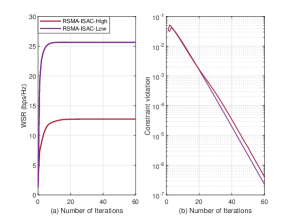
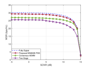
Fig. 3 depicts the convergence performance of the proposed WMMSE-PDD algorithm. Specifically, Fig. 3(a) shows the value of the OF (15a) versus the number of outer iterations of Algorithm 2 for two distinct types of channel conditions. It can be seen that both converge within 20 iterations. Fig. 3(b) illustrates the corresponding value of the constraint violation, which can be seen to be below $10^{-6}$ after 60 iterations. It can be seen from the figures that the proposed WMMSE-PDD algorithm has rapid convergence and is feasible for solving the original problem. Furthermore, the significant difference in WSR under two distinct types of channel conditions suggests that LoS components with different spatial angles can provide greater spatial degrees of freedom (DoF) to the user and improve the communication performance of the system. To verify the superiority of the proposed WMMSE-PDD algorithm, we compare it in Fig. 3 with the following benchmark algorithms: 1) the Consensus-ADMM algorithm [30], which is a distributed optimization method; and 2) the “Two-Stage” algorithm[25], which seeks to minimize the Euclidean distance of the optimal fully-digital beamforming matrix. It can be seen from Fig. 3 that, the proposed algorithm outperforms the above two benchmark algorithms in terms of the communication-sensing achievable performance region.

V-B Performance Comparison of Different Schemes

In this subsection, to verify the superiority of the proposed RSMA-assisted mmWave ISAC scheme, we consider the benchmark schemes for comparison as follows:

Refer to caption
Figure 2: Convergence performance of the proposed WMMSE-PDD algorithm.
Refer to caption
Figure 3: WSR by different methods versus sensing SCNR.
  • 1)

    SDMA-assisted ISAC: This scheme is based on a conventional multiple-access strategy with multi-user linear precoding (MU-LP) [34], in which each user decodes the desired message by treating the interference from the other user’s data streams as noise. Specifically, the SDMA-assisted ISAC scheme can be realized by disabling the common data stream in Eq. (1).

  • 2)

    NOMA-assisted ISAC: This scheme is based on a multiple access strategy with power domain superposition coding at the transmitter side and SIC at the user side [46]. Specifically, the decoding order $\pi$ is obtained based on the descending order of user channel strengths. Thus, the message of user-$\pi(k)$, $k\geq j$, is decoded at user-$\pi(j)$ using the SIC, and the corresponding SINR, denoted by $\gamma_{\pi(j)\rightarrow\pi(k)}$, can be given by

    $\displaystyle\gamma_{\pi(j)\rightarrow\pi(k)}=\frac{\left|\mathbf{h}_{\pi(j)}^{H}\mathbf{F}_{\rm RF}\mathbf{f}_{{\rm D},\pi(k)}\right|^{2}}{\sum\limits_{i<k,i\in\mathcal{K}}\left|\mathbf{h}_{\pi(j)}^{H}\mathbf{F}_{\rm RF}\mathbf{f}_{{\rm D},\pi(i)}\right|^{2}+\sigma_{{j}}^{2}}.$ (57)

    Further, the HBF problem for NOMA-assisted ISAC can be given as follows:

    $\displaystyle\textbf{{{P}}4:}\max_{\boldsymbol{\rm F}_{\rm RF},\boldsymbol{\rm F}_{\rm D}}$ $\displaystyle\sum_{k\in\mathcal{K}}\alpha_{\pi(k)}R_{\pi(k)}$ (58a)
    s.t. (15b)(15f),italic-(15bitalic-)italic-(15fitalic-)\displaystyle\eqref{SCNR}-\eqref{units}, (58b)

    where $R_{\pi(k)}=\min_{j\leq k,j\in\mathcal{K}}\{\log_{2}(1+\gamma_{\pi(j)\rightarrow\pi(k)})\}$. Problem P4 is still solved using the proposed WMMSE-PDD algorithm.

Refer to caption
Figure 4: WSR $R_{\rm WSR}$ versus power budget $P_{T}$, where $\gamma_{0}=10\ {\rm dB}$.
Refer to caption
Figure 5: WSR $R_{\rm WSR}$ versus sensing SCNR $\gamma_{0}$, where $P_{T}=30\ {\rm dBm}$.

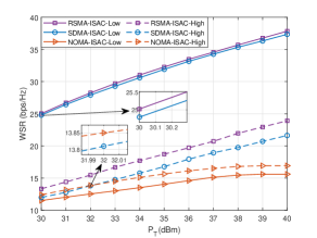
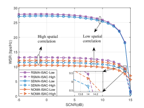
Fig. 4 shows user WSR versus budget power for different schemes with fixed sensing SCNR. For low spatial correlation channels, it can be seen that the WSR of the RSMA-ISAC scheme is slightly higher than that of the SDMA-ISAC scheme but significantly higher than that of the NOMA-ISAC scheme. Its reason is that under the high spatial DoF of mmWave channels configured with massive antennas, the strategy that makes sure that the strong user can fully decode the weak user message in the NOMA scheme will lead to the loss of multiplexing gain and rate. For the high spatial correlation channel, it can be seen that at lower budget power, the WSR of the schemes is ranked from high to low as follows: RSMA-ISAC, NOMA-ISAC, and SDMA-ISAC, but as the budget power increases, the SDMA-ISAC scheme outperforms the NOMA-ISAC. In summary, the common data stream of our proposed RSMA-ISAC scheme can reduce interference between users and further improve WSR.

Refer to caption
Figure 6: Transmit beampatterns for low spatial correlation channels.
Refer to caption
Figure 7: Transmit beampatterns for high spatial correlation channels.

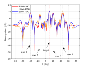
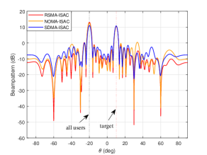
Fig. 5 depicts user WSR versus sensing SCNR thresholds for different schemes. First, when the sensing SCNR threshold is lower than $0\ {\rm dB}$, the WSR remains constant for all schemes, which indicates that there are sufficient resources to serve multiuser communication with low sensing performance requirements. Next, for the two distinct types of channel scenarios, it is observed that RSMA-ISAC schemes both achieve the largest communication-sensing performance region, which indicates that the RSMA scheme’s common data stream can also further manage the interference between radar sensing and communication, providing a greater DoF for the system’s sensing function. Note that when the sensing performance is extremely demanding, i.e., $\gamma_{0}=15\ {\rm dB}$ in the figure, the WSR of the NOMA-ISAC scheme outperforms both RSMA-ISAC and NOMA-ISAC, which is attributed to the fact that the SIC decoding strategy is used for each user in the NOMA scheme, which also provides a certain performance gain in the case of scarce communication resources. Overall, our proposed RSMA-ISAC scheme achieves better performance trade-offs and the largest achievable performance region.

Figs. 6 and 7 show the transmit beampatterns of the different schemes under the power budget $P_{T}=30\ {\rm dBm}$ and the sensing SCNR threshold $\gamma_{0}=10\ {\rm dB}$. Specifically, the transmit beampattern is defined as follows: $P(\theta)=10\log_{10}\big{(}\mathbf{a}_{t}^{H}(\theta)\boldsymbol{\rm F}_{\rm RF}\boldsymbol{\rm F}_{\rm D}\boldsymbol{\rm F}_{\rm D}^{H}\boldsymbol{\rm F}_{\rm RF}^{H}\mathbf{a}_{t}(\theta)\big{)}$. For the low spatial correlation channel, Fig. 6 depicts that all three different schemes are able to form high-gain beams on the target spatial angle $\theta_{0}=10^{\circ}$, but only the RSMA-ISAC scheme has the deepest beam depression in the four clutter directions. In addition, due to the sparsity of the mmWave channel, directional beams are also formed in the spatial directions of the four user LoS components, but among them, the user beams of the RSMA-ISAC are more stable than those of the NOMA. For the high spatial correlation channel, Fig. 7 similarly depicts that high gain beams can be formed in the target direction, but the SDMA-ISAC scheme has the weakest resistance to clutter interference. And a directional beam is formed in the direction where the spatial angles of all four user LoS components are the same, with RSMA-ISAC having the best beam performance. In summary, the RSMA-ISAC scheme has stronger anti-clutter interference and more stable multi-beam formation capability.

Refer to caption
Figure 8: Normalized beampattern of the common data streams.

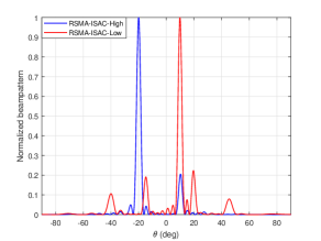
Fig. 8 depicts the spatial power distribution of the common data stream in the RSMA-ISAC scheme to further reveal the role of the common data stream in the ISAC system. The normalized beampattern is defined as follows:

$\displaystyle P(\theta_{i})=\frac{\left|\mathbf{a}_{t}^{H}(\theta_{i})\boldsymbol{\rm F}_{\rm RF}\boldsymbol{\rm f}_{\rm c}\right|^{2}}{\max_{\theta_{i}\in\Theta}\left|\mathbf{a}_{t}^{H}(\theta_{i})\boldsymbol{\rm F}_{\rm RF}\boldsymbol{\rm f}_{\rm c}\right|^{2}},\theta_{i}\in\Theta,$ (59)

where $\Theta=[-\frac{\pi}{2}:\frac{\pi}{180}:\frac{\pi}{2}]$ is the angle grid. For low spatial correlation channels, the common data stream concentrates on the power mainly in the direction of the target spatial angle, which further improves the sensing capability of the ISAC system. On the other hand, for high spatial correlation channels, the common data stream concentrates on the power in the spatial angle where all the user LoS components are the same, i.e., $\theta_{1,k}=-20^{\circ},k\in\mathcal{K}$, which serves to mitigate the interference among the dense users. Therefore, the above analysis further verifies that the common data stream has the role of both mitigating multiuser interference and the trade-off between communication and sensing performance.

Refer to caption
Figure 9: WSR $R_{\rm WSR}$ versus sensing SCNR $\gamma_{0}$.
Refer to caption
Figure 10: Energy efficiency versus sensing SCNR $\gamma_{0}$.

V-C Hybrid Beamforming Performance of RSMA-ISAC with Finite-Resolution Phase Shifters

In this subsection, we analyse the trade-offs between the WSR and energy efficiency of the communication versus the sensing SCNR thresholds in the RSMA-ISAC system under different numbers of RF chains and phase shifter phase quantization bits, respectively. Energy efficiency is defined as the ratio between WSR and total power consumption and is given by [47]:

$\displaystyle{\rm e}=\frac{R_{\rm WSR}}{P_{T}+N_{\rm RF}P_{\rm RF}+N_{\rm PS}P_{\rm PS}(b)+P_{\rm BB}}({\rm{bps/Hz/W}}),$ (60)

where $P_{\rm RF}$ denotes the power consumption of each RF chain, $P_{\rm PS}(b)$ is the power consumption of each PS with $b$-bit resolution, and $P_{\rm BB}$ is the baseband power consumption. $N_{\rm PS}$ is the total number of PSs, where $N_{\rm PS}=0$ for fully digital structures and $N_{\rm PS}=N_{t}N_{\rm RF}$ for hybrid structures. In the simulation, we adopt typical values of $P_{\rm RF}=300\ {\rm mW}$ and $P_{\rm BB}=200\ {\rm mW}$ [47]. The power consumption values of each PS are $2.5$, $5$, and $11.7\ {\rm mW}$ for 1-, 2-, and 4-bit resolution phase shifting [48]. Then $P_{\rm PS}(\infty)=17.6\ {\rm mW}$ for each infinite-resolution PS [49].

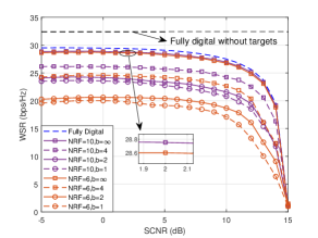
From Fig. 9, it can be seen that the WSR versus SCNR achievable performance region of the RSMA-ISAC system based on the WMMSE-PDD algorithm becomes larger with the increase in the number of RF chains and the number of phase quantization bits. When $b$ tends to infinity, the increase of RF chains improves WSR very little, but the achievable performance region of the hybrid structure has reached more than $98\%$ of the fully digital structure. Next, From Fig. 10, it is observed that the energy efficiencies at fixed perceived SCNR thresholds are consistently higher for the scenario with the number of RF chains $N_{\rm RF}=6$ compared to $N_{\rm RF}=10$, and all hybrid structures have higher energy efficiency than the fully digital structure. In this example, when the sensing SCNR is less than $11\ {\rm dB}$, the energy efficiency of the communication increases with the decrease in the number of phase quantization bits, but when the SCNR is greater than $13\ {\rm dB}$, the energy efficiency of the case “$N_{\rm RF}=6,b=\infty$” is the highest. In summary, the RSMA-ISAC with the HBF structure can achieve favorable performance trade-offs and greatly improve the energy efficiency of the system.

VI Conclusions

In this paper, we have investigated the problem of joint common rate allocation and HBF design for the RSMA-assisted mmWave ISAC system. We have proposed the WMMSE-PDD algorithm to solve this nonlinear and nonconvex optimization problem with coupled constraints. Specifically, the original problem was first transformed into an equivalent WMMSE problem, and then the PDD algorithm based on inner and outer double-layer loops solved the transformed problem. The proposed WMMSE-PDD algorithm converged to the KKT point of the original problem. In addition, we have extended the proposed algorithm to the HBF design based on the finite-resolution PSs to further improve the energy efficiency of the system. Simulation results demonstrated that the performance of the RSMA-ISAC scheme outperforms both the SDMA-ISAC and NOMA-ISAC schemes. Our proposed HBF-based RSMA-assisted mmWave ISAC system has the advantages of higher energy efficiency, more robust interference management, and better communication-sensing performance trade-offs.

Appendix A Proof of Proposition 1

First, we give the Lagrangian function for problem P2-1 as follows:

$\displaystyle\mathcal{L}=$ $\displaystyle\sum_{k\in\mathcal{K}}\alpha_{k}(\eta_{k}-C_{k})+\sum_{k\in\mathcal{K}}\lambda^{(1)}_{k}\big{(}\boldsymbol{\rm 1}^{T}\boldsymbol{\rm c}+\min_{u_{c,k},w_{c,k}}(\eta_{c,k})-g\big{)}$ (61)
$\displaystyle-\sum_{k\in\mathcal{K}}\lambda^{(2)}_{k}C_{k}+\mathcal{H},$

where $\mathcal{H}=\lambda^{(3)}\big{(}\gamma_{0}-\phi(\boldsymbol{\rm F}_{\rm RF},\boldsymbol{\rm F}_{\rm D})\big{)}+\lambda^{(4)}\big{(}\left\|\boldsymbol{\rm F}_{\rm RF}\boldsymbol{\rm F}_{\rm D}\right\|_{F}^{2}-P_{T}\big{)}+\sum_{i=1}^{N_{t}}\sum_{j=1}^{N_{\rm RF}}\lambda^{(5)}_{i,j}\big{(}\left|\boldsymbol{\rm F}_{\rm RF}(i,j)\right|-1\big{)}$. $\phi(\boldsymbol{\rm F}_{\rm RF},\boldsymbol{\rm F}_{\rm D})$ denotes the left part of the inequality sign of constraint (15b). $\boldsymbol{\lambda}=[\lambda^{(1)}_{1},\cdots,\lambda^{(1)}_{K},,\lambda^{(2)}_{1},\cdots,\lambda^{(2)}_{K},\lambda^{(3)},\lambda^{(4)},$ $\lambda^{(5)}_{1,1},\cdots,\lambda^{(5)}_{N_{t},N_{\rm RF}}]^{T}$ denote the corresponding Lagrangian multipliers. Suppose $\{\boldsymbol{\rm F}_{\rm RF}^{\star},\boldsymbol{\rm F}_{\rm D}^{\star},\boldsymbol{\rm c}^{\star},\boldsymbol{\rm u}^{\star},\boldsymbol{\rm w}^{\star}\}$ is the optimal KKT solution to problem P2-1, then it must exist that the optimal $\boldsymbol{\lambda}$ satisfies the KKT conditions as follows:

$\displaystyle\big{(}$ $\displaystyle\sum_{k\in\mathcal{K}}\alpha_{k}\nabla_{\boldsymbol{\rm F}_{\rm RF}}\eta_{k}+\sum_{k\in\mathcal{K}}\lambda^{(1)}_{k}\nabla_{\boldsymbol{\rm F}_{\rm RF}}\eta_{c,k}+\nabla_{\boldsymbol{\rm F}_{\rm RF}}\mathcal{H}\big{)}\big{|}_{\boldsymbol{\rm F}_{\rm RF}=\boldsymbol{\rm F}_{\rm RF}^{\star}}=0,$ (62a)
$\displaystyle\big{(}$ $\displaystyle\sum_{k\in\mathcal{K}}\alpha_{k}\nabla_{\boldsymbol{\rm F}_{\rm D}}\eta_{k}+\sum_{k\in\mathcal{K}}\lambda^{(1)}_{k}\nabla_{\boldsymbol{\rm F}_{\rm D}}\eta_{c,k}+\nabla_{\boldsymbol{\rm F}_{\rm D}}\mathcal{H}\big{)}\big{|}_{\boldsymbol{\rm F}_{\rm D}=\boldsymbol{\rm F}_{\rm D}^{\star}}=0,$ (62b)
$\displaystyle-\alpha_{k}+\sum_{i\in\mathcal{K}}\lambda^{(1)}_{i}-\lambda^{(2)}_{k}=0,k\in\mathcal{K},$ (62c)
$\displaystyle\alpha_{k}\frac{\partial\eta_{k}}{\partial w_{k}}\big{|}_{w_{k}=w_{k}^{\star}}=0,\ \lambda^{(1)}_{k}\frac{\partial\eta_{c,k}}{\partial w_{c,k}}\big{|}_{w_{c,k}=w_{c,k}^{\star}}=0,$ (62d)
$\displaystyle\alpha_{k}\frac{\partial\eta_{k}}{\partial u_{k}}\big{|}_{u_{k}=u_{k}^{\star}}=0,\ \lambda^{(1)}_{k}\frac{\partial\eta_{c,k}}{\partial u_{c,k}}\big{|}_{u_{c,k}=u_{c,k}^{\star}}=0,$ (62e)
$\displaystyle\lambda^{(1)}_{k}\big{(}\boldsymbol{\rm 1}^{T}\boldsymbol{\rm c}^{\star}+\min_{u_{c,k},w_{c,k}}(\eta_{c,k})-g\big{)}=0,k\in\mathcal{K},$ (62f)
$\displaystyle\lambda^{(2)}_{k}C_{k}^{\star}=0,k\in\mathcal{K},\ \lambda^{(3)}\big{(}\gamma_{0}-\phi(\boldsymbol{\rm F}_{\rm RF}^{\star},\boldsymbol{\rm F}_{\rm D}^{\star})\big{)}=0,$ (62g)
$\displaystyle\lambda^{(4)}\big{(}\left\|\boldsymbol{\rm F}_{\rm RF}^{\star}\boldsymbol{\rm F}_{\rm D}^{\star}\right\|_{F}^{2}-P_{T}\big{)}=0,\lambda^{(5)}_{i,j}\big{(}\left|\boldsymbol{\rm F}_{\rm RF}^{\star}(i,j)\right|-1\big{)}=0.$ (62h)

When the optimal solutions $w_{k}^{\star}$, $w_{c,k}^{\star}$, $u_{k}^{\star}$, and $u_{c,k}^{\star}$ take the values of $w_{k}^{\rm MMSE}$, $w_{c,k}^{\rm MMSE}$, $u_{k}^{\rm MMSE}$, and $u_{c,k}^{\rm MMSE}$, respectively, which precisely satisfy the stationarity conditions, i.e., Eqs. (62d) and (62e), and also further satisfy the rate-WMMSE relationships in Eqs. (22) and (23). Thus, it can be deduced that the gradient relationships hold as follows:

$\displaystyle\nabla_{\boldsymbol{\rm F}_{\rm RF}}R_{k}=-\nabla_{\boldsymbol{\rm F}_{\rm RF}}\eta_{k}(w_{k}^{\star},u_{k}^{\star}),$
$\displaystyle\nabla_{\boldsymbol{\rm F}_{\rm RF}}R_{c,k}=-\nabla_{\boldsymbol{\rm F}_{\rm RF}}\eta_{c,k}(w_{c,k}^{\star},u_{c,k}^{\star}),$ (63a)
$\displaystyle\nabla_{\boldsymbol{\rm F}_{\rm D}}R_{k}=-\nabla_{\boldsymbol{\rm F}_{\rm D}}\eta_{k}(w_{k}^{\star},u_{k}^{\star}),$
$\displaystyle\nabla_{\boldsymbol{\rm F}_{\rm D}}R_{c,k}=-\nabla_{\boldsymbol{\rm F}_{\rm D}}\eta_{c,k}(w_{c,k}^{\star},u_{c,k}^{\star}).$ (63b)

By substituting Eqs. (63a), (63b), and (22) into Eqs. (62a), (62b), and (62f), respectively, the following results are obtained:

$\displaystyle\big{(}-\sum_{k\in\mathcal{K}}\alpha_{k}\nabla_{\boldsymbol{\rm F}_{\rm RF}}R_{k}-\sum_{k\in\mathcal{K}}\lambda^{(1)}_{k}\nabla_{\boldsymbol{\rm F}_{\rm RF}}R_{c,k}$
$\displaystyle+\nabla_{\boldsymbol{\rm F}_{\rm RF}}\mathcal{H}\big{)}\big{|}_{\boldsymbol{\rm F}_{\rm RF}=\boldsymbol{\rm F}_{\rm RF}^{\star}}=0,$ (64a)
$\displaystyle\big{(}-\sum_{k\in\mathcal{K}}\alpha_{k}\nabla_{\boldsymbol{\rm F}_{\rm D}}R_{k}-\sum_{k\in\mathcal{K}}\lambda^{(1)}_{k}\nabla_{\boldsymbol{\rm F}_{\rm D}}R_{c,k}$
$\displaystyle+\nabla_{\boldsymbol{\rm F}_{\rm D}}\mathcal{H}\big{)}\big{|}_{\boldsymbol{\rm F}_{\rm D}=\boldsymbol{\rm F}_{\rm D}^{\star}}=0,$ (64b)
$\displaystyle\lambda^{(1)}_{k}\big{(}\boldsymbol{\rm 1}^{T}\boldsymbol{\rm c}^{\star}-R_{c,k}\big{)}=0,k\in\mathcal{K}.$ (64c)

It can be checked that the set of Eqs. (64a), (64b), (62c), (62g), (62h), and (64c) constitutes exactly the KKT conditions of Problem P1. Hence, the proof is complete.

Appendix B Proof of Proposition 2

The Lagrange function of subproblem (27) can be expressed as follows:

$\displaystyle\mathcal{L}_{1}=$ $\displaystyle\|\boldsymbol{\rm X}-\boldsymbol{\rm Y}+\rho\boldsymbol{\rm\Lambda}_{1}\|_{F}^{2}+v_{1}\big{(}f_{1}(\boldsymbol{\rm Y})-\hat{f}_{2}(\boldsymbol{\rm Y},\boldsymbol{\rm Y}^{(t)})\big{)},$ (65)

where $v_{1}\geq 0$ denotes Lagrange multiplier. Then, the KKT conditions for subproblem (37) can be given by

$\displaystyle\nabla_{\boldsymbol{\rm Y}}\mathcal{L}_{1}=-2(\boldsymbol{\rm X}-\boldsymbol{\rm Y}+\rho\boldsymbol{\rm\Lambda}_{1})+2v_{1}(\gamma_{0}\boldsymbol{\rm\Omega}\boldsymbol{\rm Y}-\boldsymbol{\rm\Phi}\boldsymbol{\rm Y}^{(t)})=0,$ (66a)
$\displaystyle v_{1}\big{(}f_{1}(\boldsymbol{\rm Y})-\hat{f}_{2}(\boldsymbol{\rm Y},\boldsymbol{\rm Y}^{(t)})\big{)}=0.$ (66b)

Hence, the optimal solution $\boldsymbol{\rm Y}^{opt}(v_{1})$ can be derived from constraint (66a), as shown in Eq.(38). Next, we discuss the Lagrange multiplier $v_{1}$ in two cases, as follows:

Case 1: if $v_{1}=0$, we can obtain the optimal solution $\boldsymbol{\rm Y}^{opt}(0)=\boldsymbol{\rm X}+\rho\boldsymbol{\rm\Lambda}_{1}$, which needs to satisfy the constraint $f_{1}(\boldsymbol{\rm Y}^{opt}(0))-\hat{f}_{2}(\boldsymbol{\rm Y}^{opt}(0),\boldsymbol{\rm Y}^{(t)})\leq 0$.

Case 2: if $v_{1}\neq 0$, the optimal solution $\boldsymbol{\rm Y}^{opt}(v_{1})$ must satisfy the equation constraint $f_{1}(\boldsymbol{\rm Y}^{opt}(v_{1}))-\hat{f}_{2}(\boldsymbol{\rm Y}^{opt}(v_{1}),\boldsymbol{\rm Y}^{(t)})=0$. First, the eigenvalue decomposition (EVD) of the Hermitian matrix $\boldsymbol{\rm\Omega}$ gives $\boldsymbol{\rm\Omega}=\boldsymbol{\rm Q}\boldsymbol{\rm\Sigma}\boldsymbol{\rm Q}^{H}$, where $\boldsymbol{\rm\Sigma}$ and $\boldsymbol{\rm Q}$ denote the diagonal matrix consisting of the eigenvalues of $\boldsymbol{\rm\Omega}$ and the unitary matrix consisting of the corresponding eigenvectors, respectively. Then, $\boldsymbol{\rm Y}^{opt}(v_{1})$ can be transformed into

$\displaystyle\boldsymbol{\rm Y}^{opt}(v_{1})=\boldsymbol{\rm Q}(\tilde{\boldsymbol{\rm\Sigma}}(v_{1}))^{-1}\boldsymbol{\rm Q}^{H}\boldsymbol{\rm D}(v_{1}),$ (67)

where $\tilde{\boldsymbol{\rm\Sigma}}(v_{1})=\boldsymbol{\rm I}_{N_{t}}+v_{1}\gamma_{0}\boldsymbol{\rm\Sigma}$ and $\boldsymbol{\rm D}(v_{1})=\boldsymbol{\rm X}+\rho\boldsymbol{\rm\Lambda}_{1}+v_{1}\boldsymbol{\rm\Phi}\boldsymbol{\rm Y}^{(t)}$. Hence, the above constraint can be rewritten as

$\displaystyle\sum_{i=1}^{N_{t}}\left[\boldsymbol{\rm E}\tilde{\boldsymbol{\rm\Sigma}}^{-1}+\tilde{\boldsymbol{\rm\Sigma}}^{-1}\boldsymbol{\rm E}^{H}\right]_{i,i}-\gamma_{0}\sum_{i=1}^{N_{t}}\left[\boldsymbol{\rm G}\tilde{\boldsymbol{\rm\Sigma}}^{-1}\boldsymbol{\rm\Sigma}\tilde{\boldsymbol{\rm\Sigma}}^{-1}\right]_{i,i}=\tilde{\gamma_{0}},$ (68)

where $\boldsymbol{\rm E}=\boldsymbol{\rm Q}^{H}\boldsymbol{\rm D}\boldsymbol{\rm Y}^{(t)H}\boldsymbol{\rm\Phi}\boldsymbol{\rm Q}$, $\boldsymbol{\rm G}=\boldsymbol{\rm Q}^{H}\boldsymbol{\rm D}\boldsymbol{\rm D}\boldsymbol{\rm Q}^{H}$, and $\tilde{\gamma_{0}}=\operatorname{tr}(\boldsymbol{\rm Y}^{(t)H}\boldsymbol{\rm\Phi}\boldsymbol{\rm Y}^{(t)})+\gamma_{0}\sigma_{z}^{2}$. Since $\boldsymbol{\rm\Sigma}$ and $\tilde{\boldsymbol{\rm\Sigma}}$ are both diagonal matrices, the optimal $v_{1}$ can be obtained by solving Eq. (68) using one-dimensional line search.

Appendix C Proof of Proposition 3

The Lagrange function of subproblem (39) can be given by

$\displaystyle\mathcal{L}_{2,k}=$ $\displaystyle\|\boldsymbol{\rm X}-\boldsymbol{\rm Z}_{k}+\rho\boldsymbol{\rm\Lambda}_{2,k}\|_{F}^{2}+\left\|\boldsymbol{\rm c}-\boldsymbol{\rm q}_{k}+\rho\boldsymbol{\rm\lambda}_{c,k}\right\|_{F}^{2}+$ (69)
$\displaystyle v_{2,k}\bigg{(}u_{c,k}\left|w_{c,k}\right|^{2}\bigg{(}\left|\boldsymbol{\rm h}_{k}^{H}\boldsymbol{\rm Z}_{k}\boldsymbol{\rm e}_{c}\right|^{2}+\sum_{i\in\mathcal{K}}\left|\boldsymbol{\rm h}_{k}^{H}\boldsymbol{\rm Z}_{k}\boldsymbol{\rm e}_{i}\right|^{2}\bigg{)}$
$\displaystyle-2u_{c,k}\mathfrak{R}\left\{w_{c,k}\boldsymbol{\rm h}_{k}^{H}\boldsymbol{\rm Z}_{k}\boldsymbol{\rm e}_{c}\right\}+\boldsymbol{\rm 1}^{T}\boldsymbol{\rm q}_{k}\bigg{)},$

where $v_{2,k}\geq 0,k\in\mathcal{K}$ is Lagrange multiplier. The KKT conditions for subproblem (39) can be written as

$\displaystyle\frac{\partial\mathcal{L}_{2,k}}{\partial\boldsymbol{\rm Z}_{k}}=0,\ \frac{\partial\mathcal{L}_{2,k}}{\partial\boldsymbol{\rm q}_{k}}=0,$ (70a)
$\displaystyle v_{2,k}\bigg{(}u_{c,k}\left|w_{c,k}\right|^{2}\bigg{(}\left|\boldsymbol{\rm h}_{k}^{H}\boldsymbol{\rm Z}_{k}\boldsymbol{\rm e}_{c}\right|^{2}+\sum_{i\in\mathcal{K}}\left|\boldsymbol{\rm h}_{k}^{H}\boldsymbol{\rm Z}_{k}\boldsymbol{\rm e}_{i}\right|^{2}\bigg{)}$
$\displaystyle-2u_{c,k}\mathfrak{R}\left\{w_{c,k}\boldsymbol{\rm h}_{k}^{H}\boldsymbol{\rm Z}_{k}\boldsymbol{\rm e}_{c}\right\}+\boldsymbol{\rm 1}^{T}\boldsymbol{\rm q}_{k}\bigg{)}=0.$ (70b)

Hence, Eqs. (40) and (41), corresponding to the optimal solutions of $\boldsymbol{\rm Z}_{k}$ and $\boldsymbol{\rm q}_{k}$, can be obtained by solving the constraint (70a). The solution of $v_{2,k}$ is also divided into two cases, $v_{2,k}=0$ and $v_{2,k}\neq 0$, which are discussed similarly to Appendix B. Therefore, we omit the solution for brevity.

Appendix D Proof of Proposition 4

We directly give the KKT conditions for subproblem (48) as follows:

$\displaystyle\sum_{k\in\mathcal{K}}\alpha_{k}u_{k}\left|w_{k}\right|^{2}\boldsymbol{\rm h}_{k}\boldsymbol{\rm h}_{k}^{H}\boldsymbol{\rm X}\sum_{i\in\mathcal{K}}\boldsymbol{\rm e}_{i}\boldsymbol{\rm e}_{i}^{H}+\big{(}v_{3}+\frac{K+2}{2\rho}\big{)}\boldsymbol{\rm X}$
$\displaystyle=$ $\displaystyle\sum_{k\in\mathcal{K}}\alpha_{k}u_{k}w_{k}^{*}\boldsymbol{\rm h}_{k}\boldsymbol{\rm e}_{k}^{H}+\frac{1}{\rho}\bigg{(}\boldsymbol{\rm Y}+\sum_{k\in\mathcal{K}}\boldsymbol{\rm Z}_{k}+\boldsymbol{\rm F}_{\rm RF}\boldsymbol{\rm F}_{\rm D}-$
$\displaystyle\rho\big{(}\boldsymbol{\rm\Lambda}_{1}+\sum_{k\in\mathcal{K}}\boldsymbol{\rm\Lambda}_{2,k}+\boldsymbol{\rm\Lambda}_{3}\big{)}\bigg{)}\triangleq\boldsymbol{\rm V},$ (71a)
$\displaystyle v_{3}\bigg{(}\operatorname{tr}\big{(}\boldsymbol{\rm X}^{H}\boldsymbol{\rm X}\big{)}-P_{T}\bigg{)}=0,$ (71b)

where $v_{3}\geq 0$ is Lagrange multiplier. Based on ${\rm vec(\boldsymbol{\rm A}\boldsymbol{\rm X}\boldsymbol{\rm B})}=(\boldsymbol{\rm B}^{T}\otimes\boldsymbol{\rm A})\rm vec(\boldsymbol{\rm X})$, constraint (71a) can be transformed into

$\displaystyle\bigg{(}\boldsymbol{\rm\Pi}+\big{(}v_{3}+\frac{K+2}{2\rho}\big{)}\boldsymbol{\rm I}_{N_{t}(K+1)}\bigg{)}\rm vec(\boldsymbol{\rm X})=\rm vec(\boldsymbol{\rm V}),$ (72)

where $\boldsymbol{\rm\Pi}=(\sum_{i\in\mathcal{K}}\boldsymbol{\rm e}_{i}\boldsymbol{\rm e}_{i}^{H})^{T}\otimes(\sum_{k\in\mathcal{K}}\alpha_{k}u_{k}\left|w_{k}\right|^{2}\boldsymbol{\rm h}_{k}\boldsymbol{\rm h}_{k}^{H})$. Then, the optimal solution for the vectorization $\boldsymbol{\rm X}$ can be obtained by Eq. (72), which is shown in Eq.(49). Next, we discuss the Lagrange multiplier $v_{3}$ based on constraint (71b).

Case 1: When $v_{3}=0$, if $\boldsymbol{\rm X}^{opt}(0)$ satisfies the constraint $\operatorname{tr}(\boldsymbol{\rm X}^{opt}(0)^{H}\boldsymbol{\rm X}^{opt}(0))\leq P_{T}$, then $\boldsymbol{\rm X}^{opt}(0)$ is the optimal solution.

Case 2: When $v_{3}\neq 0$, the optimal solution $\boldsymbol{\rm x}^{opt}(v_{3})$ must satisfy the constraint $\boldsymbol{\rm x}^{opt}(v_{3})^{H}\boldsymbol{\rm x}^{opt}(v_{3})=P_{T}$. Next, for the EVD of matrix $\boldsymbol{\rm\Pi}$, we have

$\displaystyle\boldsymbol{\rm\Pi}=\boldsymbol{\rm U}{\rm diag}\{a_{1},\cdots,a_{i},\cdots,a_{N_{t}(K+1)}\}\boldsymbol{\rm U}^{H},$ (73)

where $a_{i}$ denotes the $i$-th eigenvalue of $\boldsymbol{\rm\Pi}$, and $\boldsymbol{\rm U}$ is the unitary matrix consisting of the corresponding eigenvectors. By taking Eq. (73) into the above constraint, it yields the following:

$\displaystyle{\rm vec}(\boldsymbol{\rm V})^{H}\bigg{(}\boldsymbol{\rm\Pi}+\big{(}\frac{K+2}{2\rho}+v_{3}\big{)}\boldsymbol{\rm I}\bigg{)}^{-2}{\rm vec}(\boldsymbol{\rm V})$ (74)
$\displaystyle=$ $\displaystyle\sum_{i=1}^{N_{t}(K+1)}\frac{d_{i}}{(a_{i}+\frac{K+2}{2\rho}+v_{3})^{2}}=P_{T},$

where $d_{i}=[\boldsymbol{\rm U}^{H}{\rm vec}(\boldsymbol{\rm V}){\rm vec}(\boldsymbol{\rm V})^{H}\boldsymbol{\rm U}]_{i,i}$. The optimal Lagrange multiplier $v_{3}$ can be easily found by solving Eq.(74) using the bisection method.

References

  • [1] F. Liu, Y. Cui, C. Masouros, J. Xu, T. X. Han, Y. C. Eldar, and S. Buzzi, “Integrated sensing and communications: Toward dual-functional wireless networks for 6G and beyond,” IEEE Journal on Selected Areas in Communications, vol. 40, no. 6, pp. 1728–1767, 2022.
  • [2] L. Zheng, M. Lops, Y. C. Eldar, and X. Wang, “Radar and communication coexistence: An overview: A review of recent methods,” IEEE Signal Processing Magazine, vol. 36, no. 5, pp. 85–99, 2019.
  • [3] J. A. Zhang, M. L. Rahman, K. Wu, X. Huang, Y. J. Guo, S. Chen, and J. Yuan, “Enabling joint communication and radar sensing in mobile networks—A survey,” IEEE Communications Surveys Tutorials, vol. 24, no. 1, pp. 306–345, 2022.
  • [4] ITU-R WP5D, “Draft New Recommendation ITU-R M. [IMT.FRAMEWORK FOR 2030 ANG BEYOND],” 2023.
  • [5] B. Li, A. P. Petropulu, and W. Trappe, “Optimum co-design for spectrum sharing between matrix completion based MIMO radars and a MIMO communication system,” IEEE Transactions on Signal Processing, vol. 64, no. 17, pp. 4562–4575, 2016.
  • [6] L. Zheng, M. Lops, X. Wang, and E. Grossi, “Joint design of overlaid communication systems and pulsed radars,” IEEE Transactions on Signal Processing, vol. 66, no. 1, pp. 139–154, 2018.
  • [7] M. Roberton and E. Brown, “Integrated radar and communications based on chirped spread-spectrum techniques,” in IEEE MTT-S International Microwave Symposium Digest, 2003, vol. 1, 2003, pp. 611–614 vol.1.
  • [8] C. Sturm and W. Wiesbeck, “Waveform design and signal processing aspects for fusion of wireless communications and radar sensing,” Proceedings of the IEEE, vol. 99, no. 7, pp. 1236–1259, 2011.
  • [9] M. F. Keskin, V. Koivunen, and H. Wymeersch, “Limited feedforward waveform design for OFDM dual-functional radar-communications,” IEEE Transactions on Signal Processing, vol. 69, pp. 2955–2970, 2021.
  • [10] F. Liu, L. Zhou, C. Masouros, A. Li, W. Luo, and A. Petropulu, “Toward dual-functional radar-communication systems: Optimal waveform design,” IEEE Transactions on Signal Processing, vol. 66, no. 16, pp. 4264–4279, 2018.
  • [11] A. Hassanien, M. G. Amin, Y. D. Zhang, and F. Ahmad, “Dual-function radar-communications: Information embedding using sidelobe control and waveform diversity,” IEEE Transactions on Signal Processing, vol. 64, no. 8, pp. 2168–2181, 2016.
  • [12] L. Chen, Z. Wang, Y. Du, Y. Chen, and F. R. Yu, “Generalized transceiver beamforming for DFRC with MIMO radar and MU-MIMO communication,” IEEE Journal on Selected Areas in Communications, vol. 40, no. 6, pp. 1795–1808, 2022.
  • [13] K. Meng, Q. Wu, S. Ma, W. Chen, K. Wang, and J. Li, “Throughput maximization for UAV-enabled integrated periodic sensing and communication,” IEEE Transactions on Wireless Communications, vol. 22, no. 1, pp. 671–687, 2023.
  • [14] B. Guo, J. Liang, B. Tang, L. Li, and H. C. So, “Bistatic MIMO DFRC system waveform design via symbol distance/direction discrimination,” IEEE Transactions on Signal Processing, vol. 71, pp. 3996–4010, 2023.
  • [15] L. Chen, F. Liu, W. Wang, and C. Masouros, “Joint radar-communication transmission: A generalized pareto optimization framework,” IEEE Transactions on Signal Processing, vol. 69, pp. 2752–2765, 2021.
  • [16] F. Liu, C. Masouros, A. Li, H. Sun, and L. Hanzo, “MU-MIMO communications with MIMO radar: From co-existence to joint transmission,” IEEE Transactions on Wireless Communications, vol. 17, no. 4, pp. 2755–2770, 2018.
  • [17] X. Liu, T. Huang, N. Shlezinger, Y. Liu, J. Zhou, and Y. C. Eldar, “Joint transmit beamforming for multiuser MIMO communications and MIMO radar,” IEEE Transactions on Signal Processing, vol. 68, pp. 3929–3944, 2020.
  • [18] C. G. Tsinos, A. Arora, S. Chatzinotas, and B. Ottersten, “Joint transmit waveform and receive filter design for dual-function radar-communication systems,” IEEE Journal of Selected Topics in Signal Processing, vol. 15, no. 6, pp. 1378–1392, 2021.
  • [19] F. Liu, Y.-F. Liu, A. Li, C. Masouros, and Y. C. Eldar, “Cramér-Rao bound optimization for joint radar-communication beamforming,” IEEE Transactions on Signal Processing, vol. 70, pp. 240–253, 2022.
  • [20] X. Wang, Z. Fei, J. Huang, and H. Yu, “Joint waveform and discrete phase shift design for RIS-assisted integrated sensing and communication system under Cramer-Rao bound constraint,” IEEE Transactions on Vehicular Technology, vol. 71, no. 1, pp. 1004–1009, 2022.
  • [21] P. Kumari, J. Choi, N. González-Prelcic, and R. W. Heath, “Ieee 802.11ad-based radar: An approach to joint vehicular communication-radar system,” IEEE Transactions on Vehicular Technology, vol. 67, no. 4, pp. 3012–3027, 2018.
  • [22] M. R. Akdeniz, Y. Liu, M. K. Samimi, S. Sun, S. Rangan, T. S. Rappaport, and E. Erkip, “Millimeter wave channel modeling and cellular capacity evaluation,” IEEE Journal on Selected Areas in Communications, vol. 32, no. 6, pp. 1164–1179, 2014.
  • [23] R. W. Heath, N. González-Prelcic, S. Rangan, W. Roh, and A. M. Sayeed, “An overview of signal processing techniques for millimeter wave MIMO systems,” IEEE Journal of Selected Topics in Signal Processing, vol. 10, no. 3, pp. 436–453, 2016.
  • [24] F. Sohrabi and W. Yu, “Hybrid digital and analog beamforming design for large-scale antenna arrays,” IEEE Journal of Selected Topics in Signal Processing, vol. 10, no. 3, pp. 501–513, 2016.
  • [25] X. Yu, J.-C. Shen, J. Zhang, and K. B. Letaief, “Alternating minimization algorithms for hybrid precoding in millimeter wave MIMO systems,” IEEE Journal of Selected Topics in Signal Processing, vol. 10, no. 3, pp. 485–500, 2016.
  • [26] A. Hassanien and S. A. Vorobyov, “Phased-MIMO radar: A tradeoff between phased-array and mimo radars,” IEEE Transactions on Signal Processing, vol. 58, no. 6, pp. 3137–3151, 2010.
  • [27] F. Liu and C. Masouros, “Hybrid beamforming with sub-arrayed MIMO radar: Enabling joint sensing and communication at mmwave band,” in ICASSP 2019 - 2019 IEEE International Conference on Acoustics, Speech and Signal Processing (ICASSP), 2019, pp. 7770–7774.
  • [28] F. Liu, C. Masouros, A. P. Petropulu, H. Griffiths, and L. Hanzo, “Joint radar and communication design: Applications, state-of-the-art, and the road ahead,” IEEE Transactions on Communications, vol. 68, no. 6, pp. 3834–3862, 2020.
  • [29] Z. Cheng and B. Liao, “Qos-aware hybrid beamforming and DOA estimation in multi-carrier dual-function radar-communication systems,” IEEE Journal on Selected Areas in Communications, vol. 40, no. 6, pp. 1890–1905, 2022.
  • [30] Z. Cheng, L. Wu, B. Wang, M. R. B. Shankar, and B. Ottersten, “Double-phase-shifter based hybrid beamforming for mmwave DFRC in the presence of extended target and clutters,” IEEE Transactions on Wireless Communications, vol. 22, no. 6, pp. 3671–3686, 2023.
  • [31] Y. Mao, O. Dizdar, B. Clerckx, R. Schober, P. Popovski, and H. V. Poor, “Rate-splitting multiple access: Fundamentals, survey, and future research trends,” IEEE Communications Surveys Tutorials, vol. 24, no. 4, pp. 2073–2126, 2022.
  • [32] H. Joudeh and B. Clerckx, “Robust transmission in downlink multiuser miso systems: A rate-splitting approach,” IEEE Transactions on Signal Processing, vol. 64, no. 23, pp. 6227–6242, 2016.
  • [33] Y. Mao, B. Clerckx, and V. O. K. Li, “Rate-splitting for multi-antenna non-orthogonal unicast and multicast transmission: Spectral and energy efficiency analysis,” IEEE Transactions on Communications, vol. 67, no. 12, pp. 8754–8770, 2019.
  • [34] C. Xu, B. Clerckx, S. Chen, Y. Mao, and J. Zhang, “Rate-splitting multiple access for multi-antenna joint radar and communications,” IEEE Journal of Selected Topics in Signal Processing, vol. 15, no. 6, pp. 1332–1347, 2021.
  • [35] L. Yin, Y. Mao, O. Dizdar, and B. Clerckx, “Rate-splitting multiple access for 6g—part II: Interplay with integrated sensing and communications,” IEEE Communications Letters, vol. 26, no. 10, pp. 2237–2241, 2022.
  • [36] P. Gao, L. Lian, and J. Yu, “Cooperative ISAC with direct localization and rate-splitting multiple access communication: A pareto optimization framework,” IEEE Journal on Selected Areas in Communications, vol. 41, no. 5, pp. 1496–1515, 2023.
  • [37] Q. Shi and M. Hong, “Penalty dual decomposition method for nonsmooth nonconvex optimization—part I: Algorithms and convergence analysis,” IEEE Transactions on Signal Processing, vol. 68, pp. 4108–4122, 2020.
  • [38] Q. Shi, M. Hong, X. Fu, and T.-H. Chang, “Penalty dual decomposition method for nonsmooth nonconvex optimization—part II: Applications,” IEEE Transactions on Signal Processing, vol. 68, pp. 4242–4257, 2020.
  • [39] M. Richards, “Principles of modern radar: Basic principles,” 2010.
  • [40] G. Cui, H. Li, and M. Rangaswamy, “MIMO radar waveform design with constant modulus and similarity constraints,” IEEE Transactions on Signal Processing, vol. 62, no. 2, pp. 343–353, 2014.
  • [41] J. Capon, “High-resolution frequency-wavenumber spectrum analysis,” Proceedings of the IEEE, vol. 57, no. 8, pp. 1408–1418, 1969.
  • [42] Q. Shi, M. Razaviyayn, Z.-Q. Luo, and C. He, “An iteratively weighted MMSE approach to distributed sum-utility maximization for a MIMO interfering broadcast channel,” IEEE Transactions on Signal Processing, vol. 59, no. 9, pp. 4331–4340, 2011.
  • [43] Q. Shi and M. Hong, “Spectral efficiency optimization for millimeter wave multiuser MIMO systems,” IEEE Journal of Selected Topics in Signal Processing, vol. 12, no. 3, pp. 455–468, 2018.
  • [44] M.-M. Zhao, Y. Cai, M.-J. Zhao, Y. Xu, and L. Hanzo, “Robust joint hybrid analog-digital transceiver design for full-duplex mmwave multicell systems,” IEEE Transactions on Communications, vol. 68, no. 8, pp. 4788–4802, 2020.
  • [45] J.-C. Chen, “Hybrid beamforming with discrete phase shifters for millimeter-wave massive MIMO systems,” IEEE Transactions on Vehicular Technology, vol. 66, no. 8, pp. 7604–7608, 2017.
  • [46] Z. Wang, Y. Liu, X. Mu, Z. Ding, and O. A. Dobre, “Noma empowered integrated sensing and communication,” IEEE Communications Letters, vol. 26, no. 3, pp. 677–681, 2022.
  • [47] B. Wang, L. Dai, Z. Wang, N. Ge, and S. Zhou, “Spectrum and energy-efficient beamspace MIMO-NOMA for millimeter-wave communications using lens antenna array,” IEEE Journal on Selected Areas in Communications, vol. 35, no. 10, pp. 2370–2382, 2017.
  • [48] K.-J. Koh and G. M. Rebeiz, “0.13-$\mu$m CMOS phase shifters for X-, Ku-, and K-band phased arrays,” IEEE Journal of Solid-State Circuits, vol. 42, no. 11, pp. 2535–2546, 2007.
  • [49] Y. Xiong, X. Zeng, and J. Li, “A frequency-reconfigurable cmos active phase shifter for 5g mm-Wave applications,” IEEE Transactions on Circuits and Systems II: Express Briefs, vol. 67, no. 10, pp. 1824–1828, 2020.