Impact of pressure anisotropy on the cascade rate of Hall-MHD turbulence with bi-adiabatic ions

Abstract

The impact of ion pressure anisotropy on the energy cascade rate of Hall-MHD turbulence with bi-adiabatic ions and isothermal electrons is evaluated in three-dimensional direct numerical simulations, using the exact law derived in Simon and Sahraoui [1]. It is shown that pressure anisotropy can enhance or reduce the cascade rate, depending on the scales, in comparison with the prediction of the exact law with isotropic pressure, by an amount that correlates well with pressure anisotropy $a_{p}=\frac{p_{\perp}}{p_{\parallel}}\neq 1$ developing in simulations initialized with an isotropic pressure (${a_{p}}_{0}=1$). A simulation with an initial pressure anisotropy, ${a_{p}}_{0}=4$, confirms this trend, yielding a stronger impact on the cascade rate, both in the inertial range and at larger scales, close to the forcing. Furthermore, a Fourier-based numerical method to compute the exact laws in numerical simulations in the full $(\ell_{\perp},\ell_{\parallel})$ scale separation plane is presented.

I Introduction

The turbulent state of fluids and plasmas (e.g., stars, nebula, stellar wind, interplanetary medium) is associated with the development of cascades of various quantities (such as energy or helicity), characterized by a constant transfer rate on a range of scales belonging to the inertial domain, where driving and dissipation are negligible. The total-energy cascade rate, for instance, can be used as a proxy of the energy dissipation, and thus of the heating rate, in a turbulent medium. It can be estimated, using "exact laws" that relate the cascade rate to the increments of the fluid moments, which are more easily measurable experimentally. Initiated by von Kármán and Howarth [2] and Kolmogorov [3] in the framework of incompressible hydrodynamics turbulence, the formalism has been extended to incompressible magnetohydrodynamics (MHD) [4, 5], Hall-MHD [6, 7, 8, 9] and two-fluids flows [10, 11], and then to various compressible regimes characterized by different equations of state [12, 13, 14, 15, 16, 17, 18, 19, 20, 21, 22, 23]. Transfer rate of quantities different from the energy have also been considered in the literature [24, 25, 22, 26, 27].

In the solar wind and other accessible natural plasmas, the exact laws have been used to estimate the heating rate using in-situ observations [28, 29, 30, 15, 31, 32, 33, 31, 34]. Since the exact laws grow in complexity when including more physical effects (e.g., compressibility, non-ideal terms in the Ohm’s law), one then must resort to numerical simulations to grasp the physics involved in each term, both for freely-decaying [35, 36, 37, 8, 18, 9, 38] and driven turbulence [39, 40].

Recently, Simon and Sahraoui [23, 1] proposed a generic derivation of the exact law for the total energy, based on the internal-energy equation, and applied it to the Hall-MHD model with either isotropic or gyrotropic pressures. This work paves the road to more realistic studies of compressible turbulence in weakly collisional plasmas, such as those of the near-Earth space where the pressure is all but isotropic [41, 42, 34]. In fluid description of plasmas, pressure anisotropy was first included by Chew et al. [43], within a MHD model, usually referred to as CGL, after the authors names, or bi-adiabatic, because the heat fluxes are neglected. In the linear approximation, this model is known to permit the development of firehose and mirror-type instabilities [44, 45]. In this paper, we propose to evaluate the cascade rate in driven-turbulence simulations of the CGL-Hall-MHD system for a proton-electron plasma, obtained by adding the Hall effect to the CGL model, with the aim to quantitatively estimate the effect of pressure anisotropy on the turbulent cascade, as described by the exact law proposed in Simon and Sahraoui [1]. The study is performed on the simulation data used in Ferrand et al. [39], complemented with a new simulation specifically designed for the present work.

Section II recalls the main formulas derived in Simon and Sahraoui [1] that are used in the rest of the paper. Section III provides a brief description of the numerical code and of the of the simulation setups. Section III.2 describes the Fourier-based method used to evaluate the exact law in the numerical simulations. Section IV summarizes the main results of the study, which are discussed in Section V.

II Exact law for Hall-MHD turbulence with bi-adiabatic ions and isothermal electrons

The exact laws for a of turbulent plasma described within the MHD and Hall-MHD approximations with a bi-adiabatic closure are derived in [1]. They should however be extended to the regime of isothermal electrons considered in the simulations used in the present study.

The CGL-Hall-MHD simulations at hand are based on the following evolution equations for the plasma density $\rho$, the fluid velocity $\boldsymbol{v}$, the magnetic field $\boldsymbol{B}$, the parallel $p_{\parallel}$ and perpendicular $p_{\perp}$ components of the gyrotropic ion pressure relatively to the local magnetic field, and the total (electron and ion) pressure tensor $\overline{\boldsymbol{P}}$, assuming an isothermal electronic pressure $p_{e}$,

$$\left\{\begin{split}\partial_{t}&\rho+\boldsymbol{\nabla}\boldsymbol{\cdot}(\rho\boldsymbol{v})=-\nu_{\rho}\Delta_{\alpha}^{4}\rho,\\ \partial_{t}&\boldsymbol{v}+\boldsymbol{v}\cdot\boldsymbol{\nabla}\boldsymbol{v}+\frac{1}{\rho}\boldsymbol{\nabla}\boldsymbol{\cdot}\overline{\boldsymbol{P}}-\frac{\boldsymbol{j}}{\rho}\times\boldsymbol{B}=\boldsymbol{f}-\nu_{v}\Delta_{\alpha}^{4}\boldsymbol{v},\\ \partial_{t}&{\boldsymbol{B}}-\boldsymbol{\nabla}\times(\boldsymbol{v}\times\boldsymbol{B})+\frac{1}{R_{i}}\boldsymbol{\nabla}\times\left(\frac{\boldsymbol{j}}{\rho}\times\boldsymbol{B}\right)-\frac{1}{R_{i}}\boldsymbol{\nabla}\times\left(\frac{1}{\rho}\boldsymbol{\nabla}p_{e}\right)=-\nu_{B}\Delta_{\alpha}^{4}\boldsymbol{B},\\ \partial_{t}&p_{\parallel}+\boldsymbol{\nabla}\boldsymbol{\cdot}(p_{\parallel}\boldsymbol{v})+2p_{\parallel}\boldsymbol{b}\boldsymbol{b}:\boldsymbol{\nabla}\boldsymbol{v}=-\nu_{p}\Delta_{\alpha}^{4}p_{\parallel},\\ \partial_{t}&p_{\perp}+\boldsymbol{\nabla}\boldsymbol{\cdot}(p_{\perp}\boldsymbol{v})+p_{\perp}\boldsymbol{\nabla}\boldsymbol{\cdot}\boldsymbol{v}-p_{\perp}\boldsymbol{b}\boldsymbol{b}:\nabla\boldsymbol{v}=-\nu_{p}\Delta_{\alpha}^{4}p_{\perp},\\ \overline{\boldsymbol{P}}&=\frac{\beta_{0}}{2}\left(p_{\perp}+p_{e}\right)\overline{\boldsymbol{I}}+\frac{\beta_{0}}{2}(p_{\parallel}-p_{\perp})\boldsymbol{b}\boldsymbol{b},\\ p_{e}&=\rho.\end{split}\right.$$ (1)

Here, $\boldsymbol{j}=\boldsymbol{\nabla}\times\boldsymbol{B}$ is the current density, $\overline{\boldsymbol{I}}$ the identity tensor and ${\boldsymbol{b}}=\frac{\boldsymbol{B}}{|{\boldsymbol{B}}|}$ the unit vector in the direction of the local magnetic field. The density, magnetic field, velocity and pressures ($p_{\parallel}$, $p_{\perp}$ and $p_{e}$) are measured in units of the equilibrium density $\rho_{0}$, mean magnetic field $B_{0}$, Alfvén speed $c_{A}=\frac{B_{0}}{\sqrt{4\pi\rho_{0}}}$, and equilibrium ion parallel pressure $p_{\parallel p_{0}}$, respectively. Furthermore, $R_{i}=\frac{L}{d_{i}}=\frac{L\sqrt{4\pi e^{2}\rho_{0}}}{m_{p}c}$, where $L$ is the unit length, $d_{i}$ the ion inertial length, $e$ the elementary charge, $c$ the light speed and $m_{p}$ the proton mass, and $\beta_{0}/2=\frac{p_{\parallel p_{0}}}{\rho_{0}c^{2}_{A}}$. The time unit is $T=\frac{L}{v_{A0}}$. The term $\boldsymbol{f}$ describes the injection of kinetic energy in the system, while the hyperdiffusive terms $\nu_{X}\Delta_{\alpha}^{4}X$ induce small-scale dissipation. Note that the electron pressure term, included in the Ohm’s law, cancels out for isentropic flows [46]. In the particular case of isothermal electrons this term reads $\boldsymbol{\nabla}\times\left(\frac{1}{\rho}\boldsymbol{\nabla}p_{e}\right)=\boldsymbol{\nabla}\times\boldsymbol{\nabla}\left(\ln{\rho}\right)=0$.

The exact law in the present setting can easily be obtained from the one derived in [1]. Here, we only recall its reduced form valid in the inertial range of stationary turbulence, where dissipative and injection terms are negligible. It writes in a compact form as:

$$-4\varepsilon_{cgl}(\boldsymbol{\ell})=\boldsymbol{\nabla}_{\boldsymbol{\ell}}\cdot\boldsymbol{\mathcal{F}}(\boldsymbol{\ell})+(\mathcal{S}(\boldsymbol{\ell})+\mathcal{S}(-\boldsymbol{\ell}))+\varepsilon_{hall}(\boldsymbol{\ell})$$ (2)

with

$$\left\{\begin{split}\boldsymbol{\mathcal{F}}(\boldsymbol{\ell})&=\langle\left(\delta\left(\rho\boldsymbol{v}\right)\cdot\delta\boldsymbol{v}+\delta\left(\rho\boldsymbol{v_{A}}\right)\cdot\delta\boldsymbol{v_{A}}+2\delta\rho\delta u\right)\delta\boldsymbol{v}\rangle+\langle-\delta\rho\delta\left(\frac{\overline{\boldsymbol{P_{*}}}}{\rho}\right)\cdot\delta\boldsymbol{v}\rangle\,\\ &-\langle\left(\delta\left(\rho\boldsymbol{v_{A}}\right)\cdot\delta\boldsymbol{v}+\delta\left(\rho\boldsymbol{v}\right)\cdot\delta\boldsymbol{v_{A}}\right)\delta\boldsymbol{v_{A}}\rangle\,,\\ \mathcal{S}(\boldsymbol{\ell})&=\langle\left(\rho\boldsymbol{v}\cdot\delta\boldsymbol{v}+\frac{1}{2}\rho\boldsymbol{v_{A}}\cdot\delta\boldsymbol{v_{A}}-\frac{1}{2}\boldsymbol{v_{A}}\cdot\delta\left(\rho\boldsymbol{v_{A}}\right)+2\rho\delta u\right)\boldsymbol{\nabla}^{\prime}\boldsymbol{\cdot}\boldsymbol{v^{\prime}}\rangle\\ &+\langle\left(-2\rho\boldsymbol{v}\cdot\delta\boldsymbol{v_{A}}-\rho\boldsymbol{v_{A}}\cdot\delta\boldsymbol{v}+\delta(\rho\boldsymbol{v})\cdot\boldsymbol{v_{A}}\right)\boldsymbol{\nabla}^{\prime}\boldsymbol{\cdot}\boldsymbol{v^{\prime}_{A}}\rangle\\ &+\langle-2\rho\delta\left(\frac{\overline{\boldsymbol{P}}}{\rho}\right):\boldsymbol{\nabla}^{\prime}\boldsymbol{v^{\prime}}\rangle+\langle\left(\delta\rho\frac{\overline{\boldsymbol{P_{*}}}}{\rho}\cdot\boldsymbol{v}-\rho\delta\left(\frac{\overline{\boldsymbol{P_{*}}}}{\rho}\right)\cdot\boldsymbol{v}\right)\cdot\frac{\boldsymbol{\nabla}^{\prime}\rho^{\prime}}{\rho^{\prime}}\rangle,\\ \varepsilon_{hall}(\boldsymbol{\ell})&=2\frac{1}{R_{i}}\langle\overline{\boldsymbol{j}\times\boldsymbol{v_{A}}}\times\delta\boldsymbol{v_{A}}-\delta(\frac{\boldsymbol{j}}{\rho}\times\boldsymbol{v_{A}})\times\overline{\rho\boldsymbol{v_{A}}}\rangle\\ &+\frac{1}{R_{i}}\langle\frac{1}{2}\left(\delta\rho\boldsymbol{v^{\prime}_{A}}\cdot\boldsymbol{v_{A}}\right)\boldsymbol{\nabla}^{\prime}\boldsymbol{\cdot}\frac{\boldsymbol{j^{\prime}}}{\rho^{\prime}}-\left(\delta\rho\frac{\boldsymbol{j^{\prime}}}{\rho^{\prime}}\cdot\boldsymbol{v_{A}}\right)\boldsymbol{\nabla}^{\prime}\boldsymbol{\cdot}\boldsymbol{v^{\prime}_{A}}\rangle,\end{split}\right.$$ (3)

In the above equation, $\varepsilon_{cgl}$ is the cascade rate associated to the total energy correlation function

$$\mathcal{R}=\frac{1}{2}\left\langle\frac{1}{2}(\rho^{\prime}+\rho)\boldsymbol{v}\cdot\boldsymbol{v^{\prime}}+\frac{1}{2}(\rho^{\prime}+\rho)\boldsymbol{v_{A}}\cdot\boldsymbol{v^{\prime}_{A}}+\rho u^{\prime}+\rho^{\prime}u\right\rangle,$$

$\boldsymbol{v_{A}}=\boldsymbol{B}/\sqrt{\rho}$ is the local Alfvén velocity,

$$\rho u=\frac{\beta_{0}}{4}\left(2p_{\perp}+p_{\parallel}\right)+\rho_{e}u_{e}$$

is the density of internal energy, including the isothermal electronic contribution $\rho_{e}u_{e}=\frac{\beta_{0}}{2}\rho\ln\rho$, and $\overline{\boldsymbol{P_{*}}}$ is the total (thermal and magnetic) pressure tensor. The operator $\left\langle\right\rangle$ indicates an ensemble average, which is generally replaced by a spatial average, assuming ergodicity to hold. As usual, $\delta\varphi$ refers to the increment of a field $\varphi$ between the two positions $\boldsymbol{x}$ and $\boldsymbol{x^{\prime}}=\boldsymbol{x}+\boldsymbol{\ell}$. Primed quantities are evaluated at the position $\boldsymbol{x^{\prime}}$. The spatial derivative $\boldsymbol{\nabla}^{\prime}$ is performed relative to the variable $\boldsymbol{x^{\prime}}$, while $\boldsymbol{\nabla}_{\boldsymbol{\ell}}$ is the spatial derivative operator in the scale space. The contributions to the exact law can be separated into the divergence of the flux density $\boldsymbol{\mathcal{F}}$ constituted of structure functions, source $\mathcal{S}$ and Hall $\varepsilon_{hall}$ terms.

To analyze the exact law (3), we define the isotropic, $p=\frac{\beta_{0}}{6}\left(2p_{\perp}+p_{\parallel}\right)+\frac{\beta_{0}}{2}\rho$, and anisotropic, $\overline{\boldsymbol{\Pi}}=\overline{\boldsymbol{P}}-p\overline{\boldsymbol{I}}$, parts of the pressure. Therefore, the exact law (3) can be split into two parts: $\varepsilon_{iso}$ and $\varepsilon_{\overline{\boldsymbol{\Pi}}}$, the latter depending on the anisotropic part of the pressure tensor $\overline{\boldsymbol{\Pi}}$, while the former does not. One writes

$$-4\varepsilon_{\overline{\boldsymbol{\Pi}}}=\boldsymbol{\nabla}_{\boldsymbol{\ell}}\cdot\boldsymbol{\mathcal{F}}_{\Pi}+\mathcal{S}_{\Pi 1}+\mathcal{S}_{\Pi 2}+\mathcal{S}_{\Pi 3}$$ (4)

with

$$\left\{\begin{split}\boldsymbol{\mathcal{F}}_{\Pi}(\boldsymbol{\ell})&=-\langle\delta\rho\delta\left(\frac{\overline{\boldsymbol{\Pi}}}{\rho}\right)\cdot\delta\boldsymbol{v}\rangle,\\ \mathcal{S}_{\Pi 1}(\boldsymbol{\ell})&=(\mathcal{S}(\boldsymbol{\ell})+\mathcal{S}(-\boldsymbol{\ell}))_{\Pi 1}=\langle 2\rho^{\prime}\delta\left(\frac{\overline{\boldsymbol{\Pi}}}{\rho}\right):\boldsymbol{\nabla}\boldsymbol{v}-2\rho\delta\left(\frac{\overline{\boldsymbol{\Pi}}}{\rho}\right):\boldsymbol{\nabla}^{\prime}\boldsymbol{v^{\prime}}\rangle,\\ \mathcal{S}_{\Pi 2}(\boldsymbol{\ell})&=(\mathcal{S}(\boldsymbol{\ell})+\mathcal{S}(-\boldsymbol{\ell}))_{\Pi 3}=\langle\rho^{\prime}\delta\left(\frac{\overline{\boldsymbol{\Pi}}}{\rho}\right)\cdot\boldsymbol{v^{\prime}}\cdot\frac{\nabla\rho}{\rho}-\rho\delta\left(\frac{\overline{\boldsymbol{\Pi}}}{\rho}\right)\cdot\boldsymbol{v}\cdot\frac{\nabla^{\prime}\rho^{\prime}}{\rho^{\prime}}\rangle,\\ \mathcal{S}_{\Pi 3}(\boldsymbol{\ell})&=(\mathcal{S}(\boldsymbol{\ell})+\mathcal{S}(-\boldsymbol{\ell}))_{\Pi 2}=\langle\delta\rho\frac{\overline{\boldsymbol{\Pi}}}{\rho}\cdot\boldsymbol{v}\cdot\frac{\boldsymbol{\nabla}^{\prime}\rho^{\prime}}{\rho^{\prime}}-\delta\rho\frac{\overline{\boldsymbol{\Pi^{\prime}}}}{\rho^{\prime}}\cdot\boldsymbol{v^{\prime}}\cdot\frac{\boldsymbol{\nabla}\rho}{\rho}\rangle.\end{split}\right.$$ (5)

When computing exact laws in numerical simulations it is important to assess their level of accuracy. For this purpose, we write the full von Kármán-Howarth-Monin (KHM) equation (i.e., by relaxing the hypotheses of statistical stationarity and scale-separation), in the form

$$\partial_{t}\mathcal{R}+\varepsilon_{cgl}-\varepsilon_{F}-\varepsilon_{D}=0.$$ (6)

where

$$\varepsilon_{F} = \frac{1}{4}\left\langle\left(\rho+\rho^{\prime}\right)\left(\boldsymbol{v}\cdot\boldsymbol{f^{\prime}}+\boldsymbol{v^{\prime}}\cdot\boldsymbol{f}\right)\right\rangle$$ (7)

$$\varepsilon_{D} = -\frac{\nu_{v}}{4}\left\langle\left(\rho+\rho^{\prime}\right)\left(\boldsymbol{v}\cdot\Delta^{\prime}_{\alpha}{}^{4}\boldsymbol{v^{\prime}}+\boldsymbol{v^{\prime}}\cdot\Delta_{\alpha}^{4}\boldsymbol{v}\right)\right\rangle-\frac{\nu_{\rho}}{4}\left\langle\left(\Delta_{\alpha}^{4}\rho+\Delta^{\prime}_{\alpha}{}^{4}\rho^{\prime}\right)\boldsymbol{v}\cdot\boldsymbol{v^{\prime}}\right\rangle$$ (8)

$$-\frac{\nu_{B}}{4}\left\langle\left(\rho+\rho^{\prime}\right)\left(\frac{1}{\sqrt{\rho^{\prime}}}\boldsymbol{v_{A}}\cdot\Delta^{\prime}_{\alpha}{}^{4}\left(\sqrt{\rho^{\prime}}\boldsymbol{v^{\prime}_{A}}\right)+\frac{1}{\sqrt{\rho}}\boldsymbol{v^{\prime}_{A}}\cdot\Delta_{\alpha}^{4}\left(\sqrt{\rho}\boldsymbol{v_{A}}\right)\right)\right\rangle$$

$$+\frac{\nu_{\rho}}{8}\left\langle\left(\rho-\rho^{\prime}\right)\left(\frac{\Delta_{\alpha}^{4}\rho}{\rho}-\frac{\Delta^{\prime}_{\alpha}{}^{4}\rho^{\prime}}{\rho^{\prime}}\right)\boldsymbol{v_{A}}\cdot\boldsymbol{v^{\prime}_{A}}\right\rangle$$

$$-\frac{\nu_{p}\beta_{0}}{8}\left\langle\frac{\rho}{\rho^{\prime}}\Delta^{\prime}_{\alpha}{}^{4}\left(2p^{\prime}_{\perp}+p^{\prime}_{\parallel}\right)+\frac{\rho^{\prime}}{\rho}\Delta_{\alpha}^{4}\left(2p_{\perp}+p_{\parallel}\right)\right\rangle$$

$$-\frac{\nu_{\rho}\beta_{0}}{8}\left\langle\left(\frac{\Delta_{\alpha}^{4}\rho}{\rho}-\frac{\Delta^{\prime}_{\alpha}{}^{4}\rho^{\prime}}{\rho^{\prime}}\right)\left(\frac{\rho}{\rho^{\prime}}\left(2p^{\prime}_{\perp}+p^{\prime}_{\parallel}\right)-\frac{\rho^{\prime}}{\rho}\left(2p_{\perp}+p_{\parallel}\right)\right)\right\rangle$$

$$-\frac{\nu_{\rho}\beta_{0}}{4}\left\langle\left(\frac{\rho^{\prime}}{\rho}+\ln\rho^{\prime}\right)\Delta_{\alpha}^{4}\rho+\left(\frac{\rho}{\rho^{\prime}}+\ln\rho\right)\Delta^{\prime}_{\alpha}{}^{4}\rho^{\prime}\right\rangle$$

hold for the injection and dissipation rates, respectively.

In fact, when computed numerically, the left-hand-side of equation (6) is not strictly zero, but amounts to a value $\zeta$ that defines the numerical errors inherent to the computation of the various terms.

III Numerical setup

III.1 Simulation model

The numerical code used here is based on equations (1). Assuming periodic boundary conditions, the Cartesian three-dimensional space variables $\{x,y,z\}$ are discretized via a Fourier pseudo-spectral method, where aliasing is suppressed by spectral truncation at $2/3$ of the maximal wavenumber. The time stepping is performed with a third-order low-storage Runge-Kutta scheme, with a prescribed time-step $\delta t$.

In the driven turbulence simulations considered here, a Langevin forcing $\boldsymbol{f}$ is added in the momentum equation (see equations (1)). In Fourier space, this forcing appears as a Dirac distribution at the smallest wave vectors of the simulation domain and reflects the injection of kinetic Alfvén waves (KAWs) with amplitudes $A_{f}$, random phases, and a wave-vector making an angle $\theta_{i}$ with the mean magnetic field. After some time, a quasi-stationary regime is established in which the sum of the perpendicular kinetic and magnetic energies fluctuates around a prescribed level. The forcing is turned on when the sum of the energies of the perpendicular kinetic and magnetic fluctuations reaches a floor level given by $93\%$ of the prescribed maximal energy $E_{max}$, and is turned off when this latter level is reached. The internal energy $u$ can, however, continue to increase, with $p_{\perp}$ increasing and $p_{\|}$ decreasing (not shown), but on a typical times scale longer than the characteristic time of the turbulence dynamics. In some runs (e.g. CGL3), the averaged pressures reach a quasi-stationary level, while in others (e.g. CGL3b), they continue to evolve, but, due to the separation in the time scales, the analysis of the transfer rate can be carried out safely.

Hyperdissipation is also added in all the dynamical equations (1) to smooth the solution at the smallest scales, while allowing the development of an inertial range extending over almost two decades of scales. Since the simulations develop spatial anisotropies with respect to the mean magnetic field taken in the $z$ direction, an anisotropy parameter $\alpha$ is introduced in the Laplacian operator $\Delta_{\alpha}=\partial^{2}_{x}+\partial^{2}_{y}+\alpha\partial^{2}_{z}$.

A summary of the parameter setup for all the reported simulations is given in Table 1. The initial conditions for the different fields are $\rho_{0}=1$, $\boldsymbol{v_{0}}=[0,0,0]$ and $\boldsymbol{B_{0}}=[0,0,1]$. The ion beta $\beta_{i0}$ and the dimensionless ion inertial length $d_{i}$ are initialized at 1. The pressure anisotropy $a_{p}=\frac{p_{\perp}}{p_{\parallel}}$ is initialized at $a_{p0}=1$ for all the runs, except CGL6 where it is set equal to 4. The runs CGL1, CGL2 and CGL3 were studied in Ferrand et al. [39], in a different framework. The data set used for each simulation is extracted at the time $t_{I}$ given in Table 1. At this time, the perpendicular magnetic energy spectrum has stabilized in a quasi-stationary regime and displays spectral exponent close to the expected values $-5/3$ and $-7/3$ in the MHD and Hall inertial ranges. respectively (Fig. 1).

Except for run CGL1 for which the driving angle is $\theta=83^{\circ}$, this angle is taken equal to $75^{\circ}$ in all the other simulations. While in the runs CGL1 and CGL2, the driving acts in the MHD range ($k_{\perp}d_{i}=0.045$), in runs CGL3 and CGL3b, it acts in the close Hall range ($k_{\perp}d_{i}=0.5$), the difference between these two simulations originating from the prescribed energy level $E_{max}$ that is four times larger in the former. Run CGL5 is initialized as CGL6, except the pressures, with the driving located in the MHD range close to the Hall range ($k_{\perp}d_{i}=0.145$).

Name	CGL1	CGL2	CGL3	CGL3B	CGL5	CGL6
Resolution	$512^{3}$	$512^{3}$	$512^{2}\times 1024$	$512^{2}\times 1024$	$512^{2}\times 1024$	$512^{2}\times 1024$
$k_{\perp}d_{i}$	0.045	0.045	0.5	0.5	0.147	0.147
$\theta_{i}$	83°	75°	75°	75°	75°	75°
$E_{max}$	$1.6\times 10^{-2}$	$1.6\times 10^{-2}$	$4.5\times 10^{-2}$	$1.125\times 10^{-2}$	$1.6\times 10^{-2}$	$1.6\times 10^{-2}$
$A_{f}$	$1.0\times 10^{-3}$	$1.0\times 10^{-3}$	$8.0\times 10^{-3}$	$4.0\times 10^{-3}$	$3.0\times 10^{-3}$	$3.0\times 10^{-3}$
$\nu_{v}=\nu_{B}$	$7.35\times 10^{-8}$	$7.35\times 10^{-8}$	$4.0\times 10^{-14}$	$1.0\times 10^{-14}$	$3.0\times 10^{-11}$	$3.0\times 10^{-11}$
$\nu_{\rho}$	0	0	$1.6\times 10^{-14}$	$1.0\times 10^{-14}$	0	0
$\nu_{p}$	$7.35\times 10^{-9}$	$7.35\times 10^{-9}$	$1.6\times 10^{-14}$	$1.0\times 10^{-14}$	$3.0\times 10^{-12}$	$3.0\times 10^{-12}$
$\alpha$	80	10	2.5	2.5	6	5
$\delta t$	$6.25\times 10^{-2}$	$5\times 10^{-2}$	$2\times 10^{-4}$	$3\times 10^{-4}$	$5\times 10^{-3}$	$5\times 10^{-3}$
$t_{I}$	6700	12900	361	410	12905	2730
$a_{p0}$	1	1	1	1	1	4

Table 1: Parameters of the various runs: $k_{\perp}d_{i}$, $\theta_{i}$, $E_{max}$, $A_{f}$

are forcing parameters (injection wavenumber, angle, threshold and amplitude, respectively), while $\nu_{v}=\nu_{B}$, $\nu_{\rho}$, $\nu_{p}$ are hyperdissipation coefficients arising in the dynamical equations for the velocity, the magnetic field, the density and the pressures, respectively. The anisotropy parameter $\alpha$ enters the definition of the anisotropic Laplacian used in the simulations. The parameters $\delta t$ and $t_{I}$ refer to the time step and to the time at which the analysis was performed, while $a_{p0}$ measures the initial pressure anisotropy.

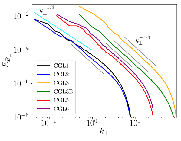
Figure 1: Power spectra of the perpendicular magnetic field for the various simulations. The expected slope in the inertial (resp. Hall) range is indicated in cyan (resp. grey). The spectra of CGL1 and CGL2 are shifted down by a factor 20, for clarity.

III.2 Pseudo-spectral calculation of the structure functions

As previously mentioned, exact laws can be written in the general form

$$-4\varepsilon(\boldsymbol{\ell})=\boldsymbol{\nabla}_{\boldsymbol{\ell}}\cdot\boldsymbol{\mathcal{F}}(\boldsymbol{\ell})+({\widetilde{\mathcal{S}}(}\boldsymbol{\ell})+{\widetilde{\mathcal{S}}}(-\boldsymbol{\ell})),$$

where $\varepsilon$ is the cascade rate and ${\widetilde{\mathcal{S}}}$ collects all the terms not included in the divergence of ${\boldsymbol{\mathcal{F}}}$.

A straightforward method to compute the exact law on the whole scale grid is to code a loop on all the possible separations $\boldsymbol{\ell}$ whose components in each direction are multiple of the mesh size in this direction, up to half the corresponding linear extension of the domain in this direction, to compute spatial derivatives with a four-point difference scheme for good accuracy, and to approximate the ensemble average by a spatial average over all the collocation points of the separation domain. However, such a procedure is extremely time- and memory-consuming. Consequently, in previous works [39, 38, 18], the computation was performed on only a fraction of scales, associated with wisely selected directions in the separation space. Here, we introduce a different method, based on the equivalence between the two-point correlation function and a convolution product. Thanks to this remark, we can compute the whole scale grid at once. Indeed, for two fields $A$ and $B$, the correlation product $\left\langle A^{\prime}\cdot B\right\rangle=\int A(\boldsymbol{x}+\boldsymbol{\ell})B(\boldsymbol{x})d\boldsymbol{x}$ can be viewed as the convolution product $A(\boldsymbol{\ell})*B(-\boldsymbol{\ell})=\int A({\boldsymbol{x}})\cdot B(-(\boldsymbol{\ell}-{\boldsymbol{x}}))d{\boldsymbol{x}}$ that can easily be done in Fourier space as a simple product of the Fourier transform of $A$ and of the complex conjugate of the Fourier transform of $B$. This protocol is possible for all terms in the source part ${\widetilde{\mathcal{S}}}$ entering the law. For the terms entering $\boldsymbol{\mathcal{F}}$, the nonlinearity of which is higher than quadratic, the procedure is to be performed iteratively. The outcome is a 3D array in the scale space.

Assuming that the scale space is axisymmetric with respect to the mean magnetic field and that all the considered statistical quantities are even in $\boldsymbol{\ell}$, 2D maps in function of $\ell_{\perp}$ and $\ell_{\parallel}>0$ are obtained by angular averaging in each perpendicular planes. These full 2D plots provide information about the cascade anisotropy in turbulence experiments [47] and numerical simulations [48]. To describe the cascade in the perpendicular direction, one may consider the 1D profiles, functions of $\ell_{\perp}$ only, which are obtained by restricting the considered quantity to the plane $\ell_{\parallel}=0$. This procedure mirrors the integration, in the Fourier space, over all the $k_{\parallel}$, in order to obtain the spectral distribution in $k_{\perp}$. Reciprocally, integration over all the parallel scales $\ell_{\parallel}$ is equivalent, in Fourier space, to considering the specific $k_{\parallel}=0$ plane. Note that, for the sake of simplicity, we keep using the same notation $\varepsilon$ for the 2D cascade rate $\varepsilon(\ell_{\perp},\ell_{\parallel})$ and the cascade rate in the perpendicular direction (in brief, perpendicular cascade rate) $\varepsilon(\ell_{\perp})=\varepsilon(\ell_{\perp},\ell_{\parallel}=0)$, as the context prevents any ambiguity.

The time derivative needed to compute $\zeta$ is obtained using a two-point finite-difference scheme around the selected time $t_{I}$ (see Table 1).

IV Results

In this section, the results of the computation of the exact law on the runs CGL1-CGL6 are analyzed. We recall that CGL1 and CGL2 cover mostly MHD scales, while CGL3 targets the smaller (Hall) scales. CGL3B is similar to CGL3 with a lower energy content, CGL5 was designed to cover the transition between the MHD and Hall ranges, by prescribing a forcing at an intermediate scale, CGL6 is similar to CGL5 except for the initial pressure anisotropy. Combined together, these simulations allow us to cover a range of scales covering more than 2.5 decades, spanning both the MHD and the sub-ion scales. We will start our analysis by considering the cascade in the perpendicular direction, before turning to the full 2D maps.

IV.1 Global contributions to the KHM equation

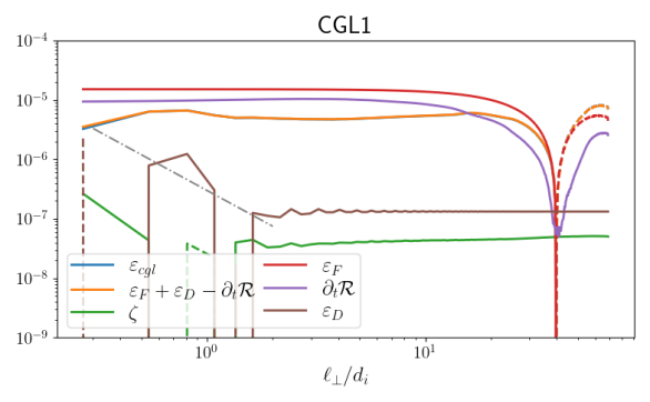
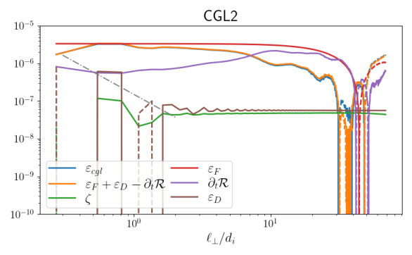
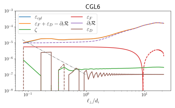
Figure 2: 1D perpendicular profiles of the various terms of equation (6) for CGL1, CGL2, CGL3 and CGL6. Here and in the similar graphs presented in the following, solid lines refer to positive quantities, and dashed lines to the absolute value of negative quantities. Note that the blue line is almost undistinguishable from the orange one, consistent with equation (6) and the low level of the error $\zeta$. A $-2$-slope tendency is added as a grey dot-dashed line.

The 1D perpendicular profiles ($\ell_{\parallel}=0$) of the various terms entering equation (6) and of the numerical error $\zeta$ are shown for CGL1, CGL2, CGL3 and CGL6 in Fig. 2. In the separation space, the forcing term $\varepsilon_{F}$ is nearly constant down to the smallest scales, consistent with a forcing in the form of a Dirac distribution in Fourier space. The term $\partial_{t}\mathcal{R}$ reflects the instantaneous time fluctuations that, as in decaying turbulence [38], do not prevent the establishment of an extended inertial range. The properties of $\varepsilon_{F}$ and $\partial_{t}\mathcal{R}$ differ in the various simulations: for CGL1 and CGL2 (and CGL3B –not shown), both terms are positive at most of the scales, for CGL3 (and CGL5 –not shown), they are mostly negative, while for CGL6, they have opposite signs.

The dissipation term $\varepsilon_{D}$ has an envelope with a slope $-2$ at the smallest scales. This reflects a divergence of the two-point correlation function of a variable that has a power-law spectrum $k^{-3}$ or steeper, which is the case of the spectra shown in Fig. 1 that steepen significantly at large wavenumber because of hyperdissipation. This issue can be overcome by using higher order correlation functions [49]. We will not further discuss the dissipation term in this paper considering that it represents about $1\%$ of $\varepsilon_{cgl}$ in the inertial range, and thus does not significantly affect the cascade rate, but at the smallest scales.

We observe that $\varepsilon_{cgl}$ (blue) coincides with $-\partial_{t}\mathcal{R}+\varepsilon_{F}+\varepsilon_{D}$ (purple) with an error $\zeta$ (brown) between $10^{-7}$ and $10^{-8}$ for CGL1 and CGL2, between $10^{-5}$ and $10^{-6}$ for CGL3 and between $10^{-6}$ and $10^{-7}$ for CGL6. The uncertainty level is thus about $1\%$ to $10\%$ of $\varepsilon_{cgl}$, which allows us to analyze, in a relatively reliable way, the various components of $\varepsilon_{cgl}$ in these simulations.

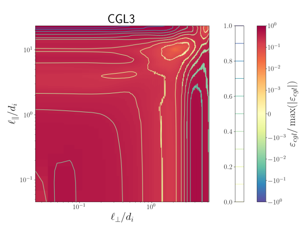
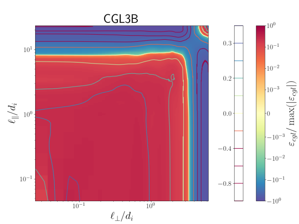
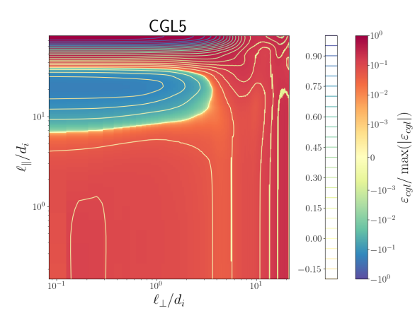
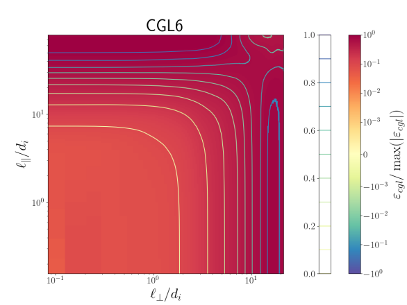
Figure 3: 2D maps of $\varepsilon_{cgl}/\max(|\varepsilon_{cgl}|)$ for CGL3 (top-left), CGL3B (top-right), CGL5 (bottom-left) and CGL6 (bottom-right). An orange-red background indicates a positive non-linear transfer and a green-blue background, a negative one. Contour lines are based on the linear scale displayed on the left of the color bar.

Figure 3 shows the resulting 2D maps of the normalized total cascade rate $\varepsilon_{cgl}$. The background colors indicate the variation of $\varepsilon_{cgl}$ with the positive values in warm colors and the negative ones in cold colors. Superimposed are a few contour lines. As visible on the perpendicular cascade rate (Fig. 2), $\varepsilon_{cgl}$ decreases slightly at small scales and vary significantly at the large ones, while displaying a positive plateau at the intermediate $(\ell_{\perp},\ell_{\parallel})$ scales. This plateau defines the inertial range. We remark that in the $(\ell_{\perp},\ell_{\parallel})$ plane, the inertial range covers a domain whose shape is close to a square because of the logarithmic axes. One also notices that the large-scale variations of $\varepsilon_{cgl}$ are quite different in the various simulations: in CGL3B and CGL5 the sign changes, while in CGL3 and CGL6 $\varepsilon_{cgl}$ is positive with an enhancement in the forcing range and, for CGL3, a slight decrease at the transition between the inertial and the forcing scales. The behavior of the cascade rate in CGL5 is similar to that in CGL3B in the perpendicular direction, including the sign variations. A possible interpretation of these features is presented in the following, by analyzing the different components of $\varepsilon_{cgl}$.

IV.2 Isotropic and anisotropic pressure-induced contributions, $\varepsilon_{iso}$ and $\varepsilon_{\overline{\boldsymbol{\Pi}}}$, to the total cascade rate $\varepsilon_{cgl}$

We now analyze in the various simulations, the partition of the total cascade rate into $\varepsilon_{\overline{\boldsymbol{\Pi}}}$, originating from the pressure anisotropy, and the isotropic contribution $\varepsilon_{iso}$. The results are shown in Fig. 4 as 1D perpendicular profiles in $\ell_{\perp}$. An estimate of the pressure-anisotropy contribution, through the signed ratio $\frac{\varepsilon_{\overline{\boldsymbol{\Pi}}}}{|\varepsilon_{cgl}|}$, is given in Fig. 5, using $(\ell_{\perp},\ell_{\|})$ 2D maps.

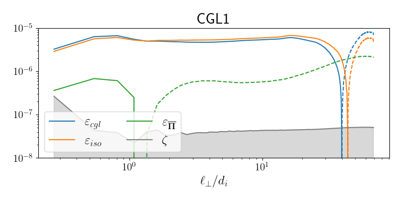
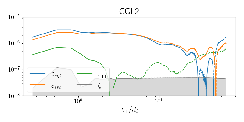
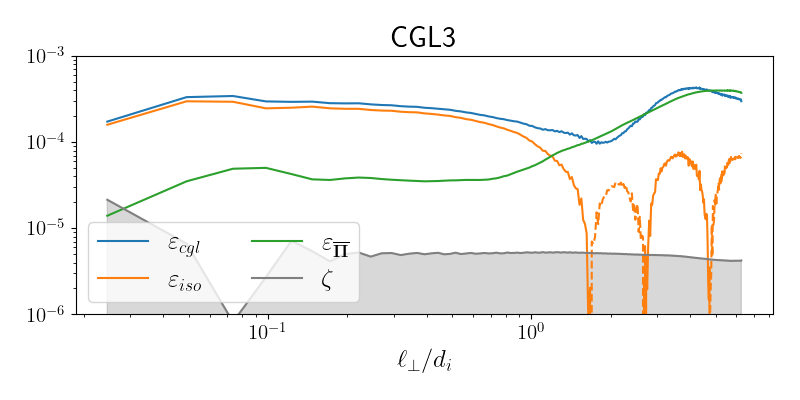
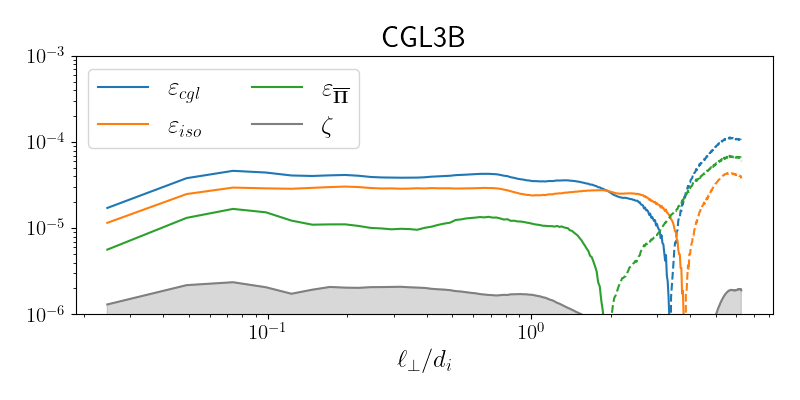
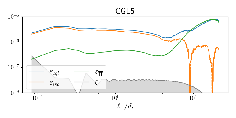
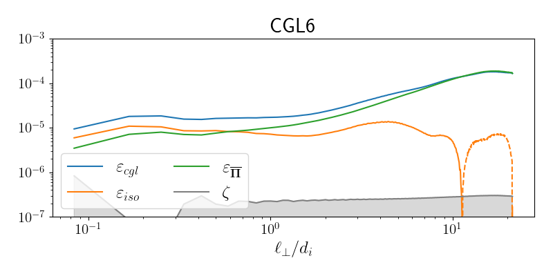
Figure 4: 1D perpendicular-cascade $\varepsilon_{cgl}$ (blue), $\varepsilon_{iso}$ (orange) and $\varepsilon_{\overline{\boldsymbol{\Pi}}}$ (green) for the various simulations. The grey areas holds for the error level.

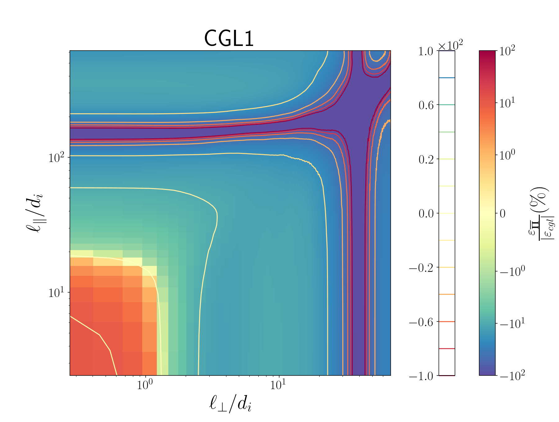
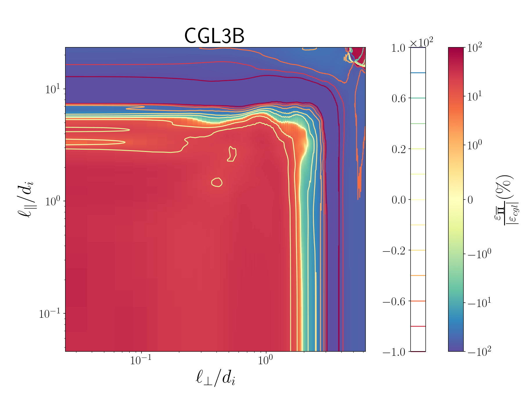
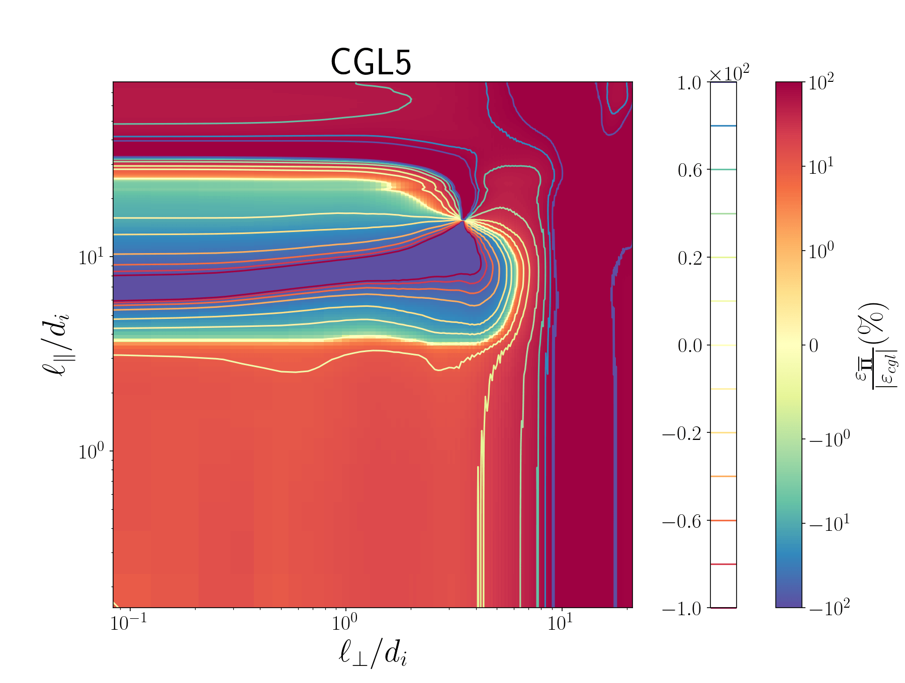
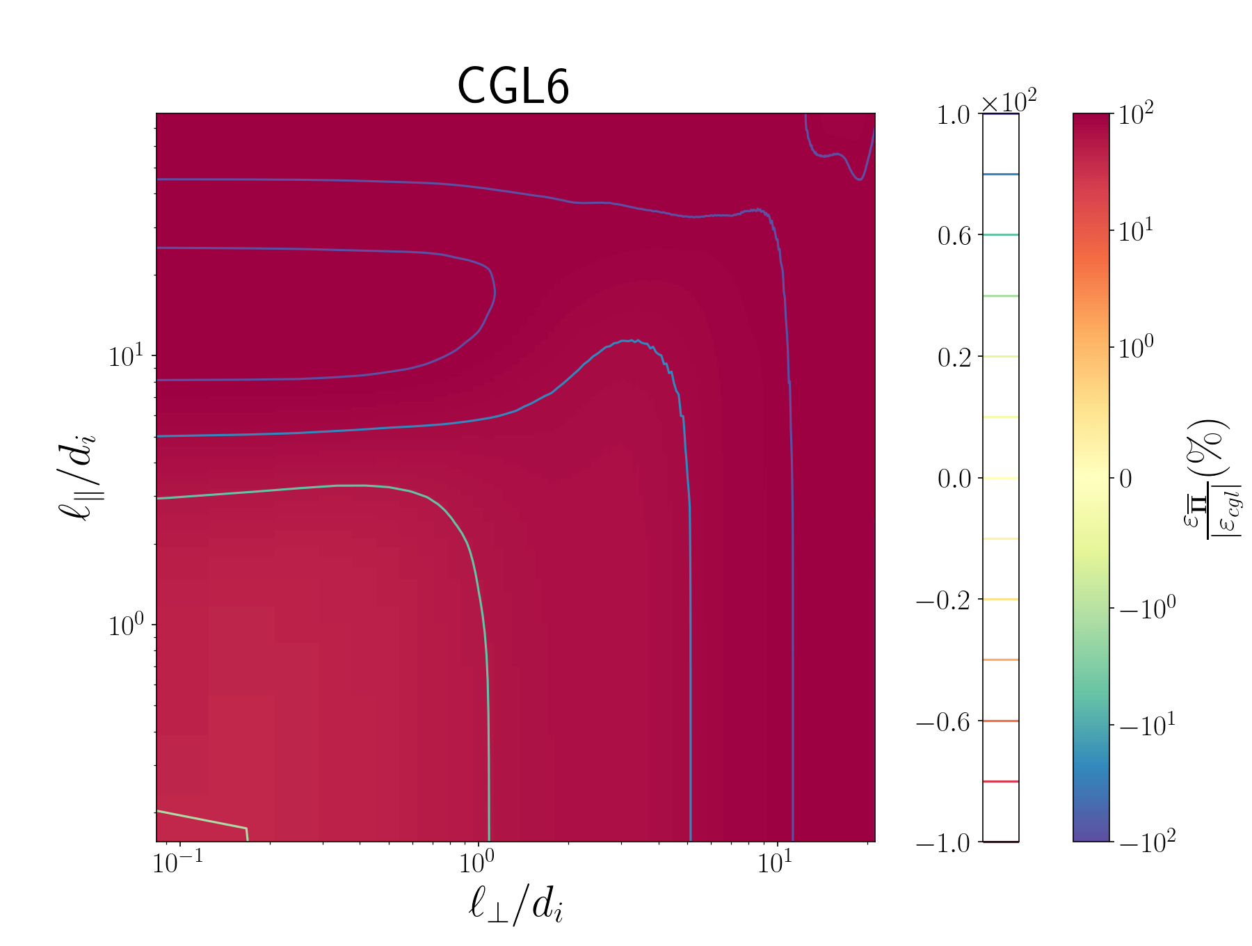
Figure 5: 2D map of $\varepsilon_{\overline{\boldsymbol{\Pi}}}/|\varepsilon_{cgl}|$ for the different runs. Warm color indicates a positive contribution of pressure anisotropy varying from 0 (yellow) to $100\%$ (red), and green-blue color, a negative contribution, while the purple domain circled by a red contour line correspond to the range where the sign of $\varepsilon_{cgl}$ fluctuates, because of the variations of $\varepsilon_{iso}$.

Figure 4 shows that the contribution of $\varepsilon_{\overline{\boldsymbol{\Pi}}}$ to the total cascade rate in the inertial range is smaller ($\varepsilon_{\overline{\boldsymbol{\Pi}}}\simeq 10\%$ of $\varepsilon_{cgl}$) for CGL1 and CGL2 than for CGL3B ($30\%$) and CGL6 ($50\%$). However, at the largest scales, close to the forcing, this contribution reaches $30-60\%$ of $\varepsilon_{cgl}$ for CGL1-2-3B, and $100\%$ for CGL3-5-6. This increase is also visible on Fig. 5, where the maps become bluer or redder at large scales. The higher level of the full cascade rate for CGL6 compared to the other runs is due to the larger initial pressure anisotropy of this run, which impacts $\varepsilon_{\overline{\boldsymbol{\Pi}}}$. One also notices the similarities in the behavior of CGL3 and CGL5. The case of CGL3B will be discussed in Section V. As confirmed by CGL5, for which the forcing scale lies between those of CGL1-2 and of CGL3B-3, the variations of the cascade rate occurs mainly at the injection scales.

As seen in Fig. 4, for CGL1, CGL2 and CGL3B, $\varepsilon_{\overline{\boldsymbol{\Pi}}}$ is positive at the smallest scales ($\ell_{\perp}/d_{i}\lesssim 1$) and negative at larger ones. The change of sign occurs in the MHD range, close to $\ell_{\perp}=d_{i}$ in the perpendicular direction, and close to the forcing scales in the parallel direction (see Fig. 5). This behavior underlines the role of the forcing in the generation of sign fluctuations for $\varepsilon_{\overline{\boldsymbol{\Pi}}}$ (and possibly for other components of the cascade rate), rather than a physical effect occurring at the specific scales where the sign change is observed. These changes of sign induce a shallow decrease of the total cascade rate and limit the extension of the inertial range close to the forcing scale. While no change of sign of $\varepsilon_{\overline{\boldsymbol{\Pi}}}$ is visible for the perpendicular cascade of CGL3 and CGL5, the cascade rate behaves differently in the parallel direction for these simulations. CGL6 shows no sign change in either direction. For all the simulations, $\varepsilon_{iso}$ and $\varepsilon_{\overline{\boldsymbol{\Pi}}}$ are significantly larger than the uncertainty level $\zeta$, indicating a negligible effect of the numerical error on the the total cascade rate.

The above results highlight the contribution of the pressure anisotropy to the cascade rate. The detailed analysis of $\varepsilon_{iso}$ and $\varepsilon_{\overline{\boldsymbol{\Pi}}}$ is performed in the following subsections.

IV.3 Contribution to $\varepsilon_{iso}$ induced by density fluctuations

Here, we compare $\varepsilon_{iso}$ that collects all the terms independent of the pressure anisotropy in $\varepsilon_{cgl}$, as obtained in the present simulations, to the predictions of the incompressible exact law used in Ferrand et al. [39], and with other results based on isotropic compressible models [18].

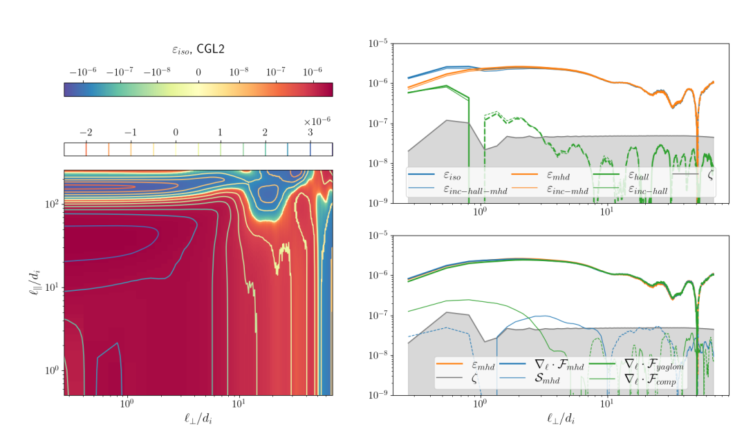
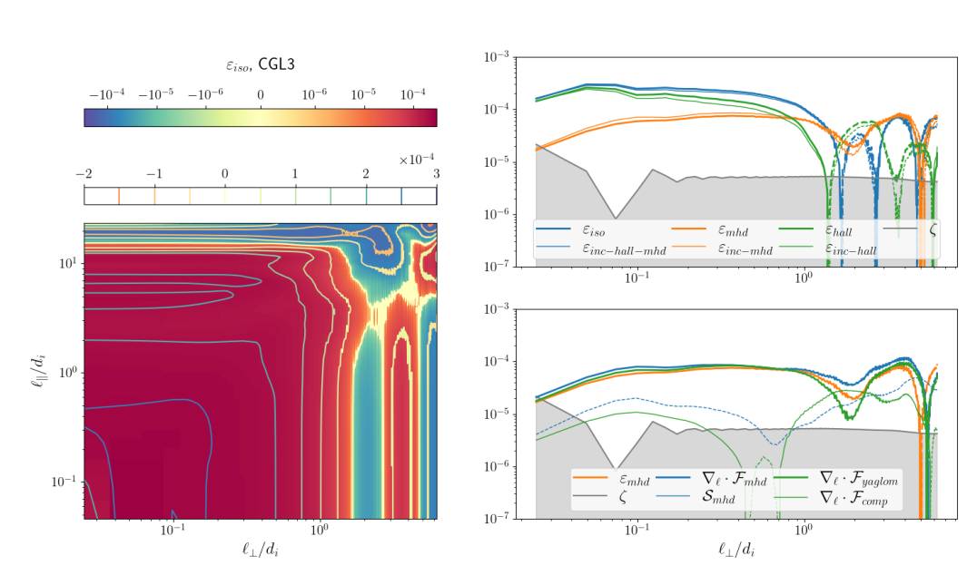
Figure 6: Left: 2D map (with same graphic conventions as in Fig. 3) of $\varepsilon_{iso}$ in the $(\ell_{\perp},\ell_{\parallel})$ plane for CGL2. Right: 1D perpendicular profiles of the various contributions to $\varepsilon_{iso}$. Top-right: comparison of the MHD ($\varepsilon_{mhd}$, thick orange) and Hall ($\varepsilon_{hall}$, thick green) contributions to $\varepsilon_{iso}$ (thick blue) with their incompressible counterparts (thin curves). Bottom-right: components of $\varepsilon_{mhd}$ (orange) i.e. the flux part (thick blue) and source part (thin blue), and detail of the flux part i.e. Yaglom part (thick green) and purely compressible part (thin green).

Figure 7: Run CGL3: representation similar to Fig. 7.

Figure 7 (resp. 7) shows the $(\ell_{\perp},\ell_{\parallel})$ 2D map of $\varepsilon_{iso}$, obtained from CGL2 (resp. CGL3). An inertial range is visible between $\ell_{\perp}\in[0.5,7]$ and $\ell_{\parallel}\in[5,90]$ (resp. $\ell_{\perp}\in[0.05,1]$ and $\ell_{\parallel}\in[0.2,10]$). At the smallest scales, $\varepsilon_{iso}$ decreases due to dissipation, and varies in sign and amplitude at the largest scales where the forcing acts. As expected, the inertial range (in the sense of a constant cascade rate) of CGL2 is evidenced in the MHD scales, while for CGL3 it is limited to the Hall scales. CGL1 (not shown) exhibits a broader inertial range in $\ell_{\perp}$ than CGL2, probably due to a more efficient generation of Alfvenic turbulence by a driving acting in a more quasi-perpendicular direction ($\theta_{i}=83^{\circ}$ for CGL1 and $75^{\circ}$ for CGL2).

These observations also hold for the 1D perpendicular cascade rate displayed in the top-right graphs of Figs. 7 and 7 (thick blue line). The profile of $\varepsilon_{iso}$ is close to that of the incompressible Hall-MHD contribution ($\varepsilon_{inc-hall-mhd}$, thin blue line), obtained with the exact law used by Ferrand et al. [9]. The MHD ($\varepsilon_{mhd}$, orange) and Hall ($\varepsilon_{hall}$, green) components are also close to their incompressible counterparts ($\varepsilon_{inc-mhd}$ and $\varepsilon_{inc-hall}$, thin lines): the difference between compressible and incompressible models vary between $1\%$ and $10\%$, and is slightly more important for CGL3. Such observations are expected, since the present simulations are only weakly compressible (for CGL2: $\frac{std(\rho)}{\left<\rho\right>}=2\%$ for CGL3: $\frac{std(\rho)}{\left<\rho\right>}=8\%$). The MHD and Hall contributions behave as expected: at scales $\ell_{\perp}\sim d_{i}$, the Hall contribution increases and overcomes the decreasing MHD one, thus ensuring a constant total cascade rate.

The various components of $\varepsilon_{mhd}$ are displayed in the bottom-right panels of Figs. 7 and 7, with $\varepsilon_{mhd}$ decomposed as $\varepsilon_{mhd}=\boldsymbol{\nabla}_{\boldsymbol{\ell}}\cdot\boldsymbol{\mathcal{F}}_{mhd}+\mathcal{S}_{mhd}$ where

$$\boldsymbol{\mathcal{F}}_{mhd}=\boldsymbol{\mathcal{F}}_{yaglom}+\boldsymbol{\mathcal{F}}_{comp}$$ (9)

with

$$\left\{\begin{split}\boldsymbol{\mathcal{F}}_{yaglom}&=-\frac{1}{4}\langle\left(\delta\left(\rho\boldsymbol{v}\right)\cdot\delta\boldsymbol{v}+\delta\left(\rho\boldsymbol{v_{A}}\right)\cdot\delta\boldsymbol{v_{A}}\right)\delta\boldsymbol{v}-\left(\delta\left(\rho\boldsymbol{v_{A}}\right)\cdot\delta\boldsymbol{v}+\delta\left(\rho\boldsymbol{v}\right)\cdot\delta\boldsymbol{v_{A}}\right)\delta\boldsymbol{v_{A}}\rangle\,,\\ \boldsymbol{\mathcal{F}}_{comp}&=-\frac{1}{4}\langle\delta\rho\left(2\delta u-\delta\left(\frac{p+p_{m}}{\rho}\right)\right)\delta\boldsymbol{v}\rangle\,\end{split}\right.$$

and

$$\mathcal{S}_{mhd}=\left(\mathcal{S}(\boldsymbol{\ell})+\mathcal{S}(-\boldsymbol{\ell})\right)$$ (10)

with

$$\left\{\begin{split}\mathcal{S}(\boldsymbol{\ell})&=\langle\left(\rho\boldsymbol{v}\cdot\delta\boldsymbol{v}+\frac{1}{2}\rho\boldsymbol{v_{A}}\cdot\delta\boldsymbol{v_{A}}-\frac{1}{2}\boldsymbol{v_{A}}\cdot\delta\left(\rho\boldsymbol{v_{A}}\right)+2\rho\delta u\right)\boldsymbol{\nabla}^{\prime}\boldsymbol{\cdot}\boldsymbol{v^{\prime}}\rangle\\ &+\langle\left(-2\rho\boldsymbol{v}\cdot\delta\boldsymbol{v_{A}}-\rho\boldsymbol{v_{A}}\cdot\delta\boldsymbol{v}+\delta(\rho\boldsymbol{v})\cdot\boldsymbol{v_{A}}\right)\boldsymbol{\nabla}^{\prime}\boldsymbol{\cdot}\boldsymbol{v^{\prime}_{A}}\rangle\\ &+\langle-2\rho\delta\left(\frac{p}{\rho}\right):\boldsymbol{\nabla}^{\prime}\boldsymbol{v^{\prime}}\rangle+\langle\left(\delta\rho\frac{p+p_{m}}{\rho}\cdot\boldsymbol{v}-\rho\delta\left(\frac{p+p_{m}}{\rho}\right)\cdot\boldsymbol{v}\right)\cdot\frac{\boldsymbol{\nabla}^{\prime}\rho^{\prime}}{\rho^{\prime}}\rangle,\end{split}\right.$$

The quantity $\boldsymbol{\nabla}\cdot\boldsymbol{\mathcal{F}}_{yaglom}$ is the part of $\varepsilon_{mhd}$ that survives when formally taking $\rho=\rho_{0}=1$, typical of an incompressible regime, yielding $\varepsilon_{inc-mhd}$, while $\boldsymbol{\nabla}\cdot\boldsymbol{\mathcal{F}}_{comp}$ will vanish in this limit. Note that $\boldsymbol{\nabla}\cdot\boldsymbol{\mathcal{F}}_{comp}$ and $\mathcal{S}_{mhd}$, referred to as hybrid and source terms in Andrés et al. [18] and Simon and Sahraoui [23], are expressed here using the structure functions. Similarly to the results reported in isothermal turbulence simulations [18], their contribution to $\varepsilon_{mhd}$ remains negligible ($1\%$ to $10\%$ at the smallest scales), an effect possibly originating from the weak compressibility of the present simulations.

Similar behavior of $\varepsilon_{iso}$ is obtained for the other simulations, in agreement with previous results published in the literature, thus validating the contribution to $\varepsilon_{cgl}$ that is independent of the pressure anisotropy.

IV.4 Detailed analysis of $\varepsilon_{\overline{\boldsymbol{\Pi}}}$

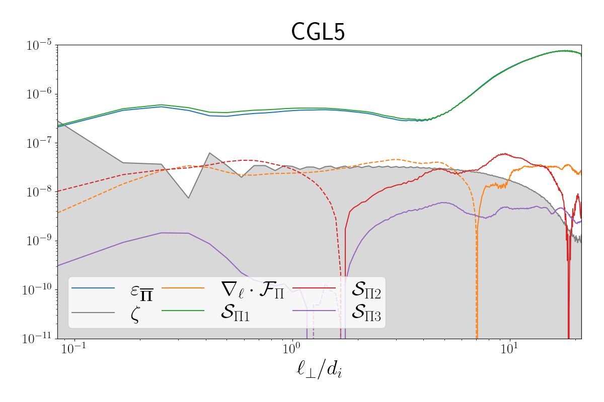
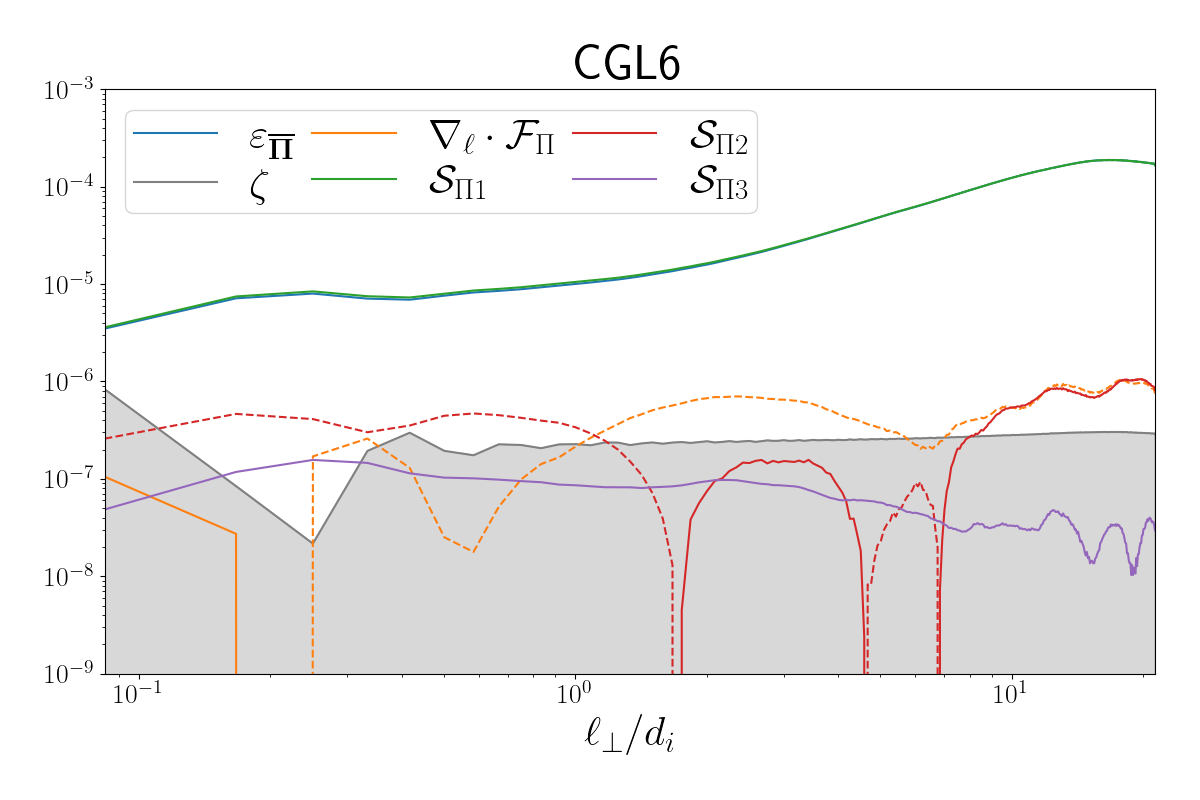
Figure 8: 1D perpendicular profile of the different contributions to $\varepsilon_{\overline{\boldsymbol{\Pi}}}$ (blue) in run CGL5 and CGL6. The source term that does not explicitly depend on the density fluctuations is plotted in green. The grey area reflects the uncertainty level $\zeta$. Plain lines are for positive values and dashed lines for negative ones.

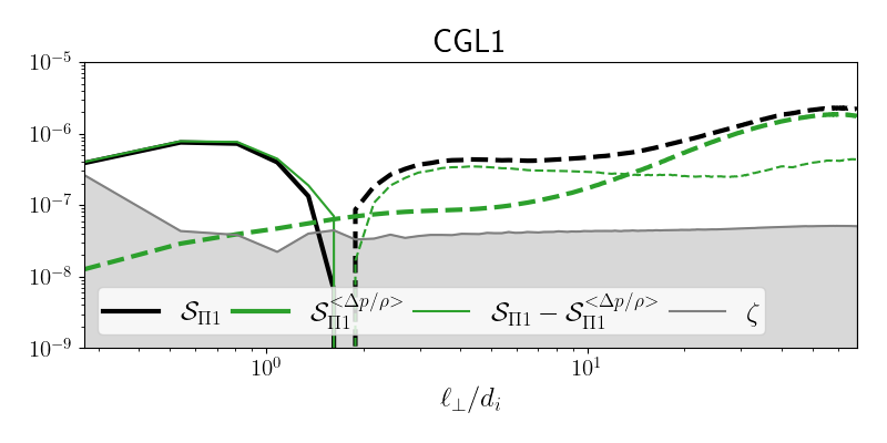
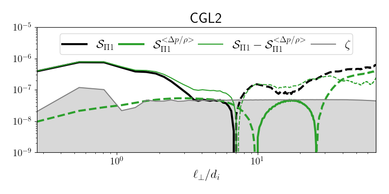
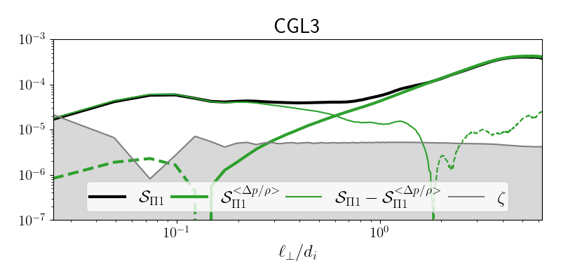
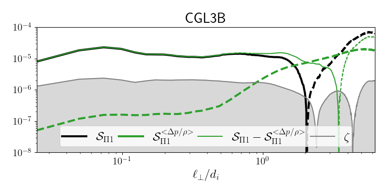
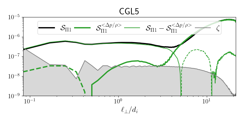
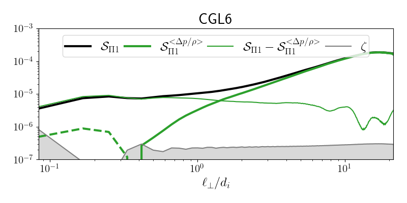
Figure 9: For each simulation, 1D perpendicular profile of the decomposition of $\mathcal{S}_{\Pi 1}$ into terms depending or not on the (mean) quantity $\left<\frac{\Delta p}{\rho}\right>=\left<\frac{p_{\parallel}-p_{\perp}}{\rho}\right>$.

All the simulations display similar results about the contributions of the different terms entering $\varepsilon_{\overline{\boldsymbol{\Pi}}}$. Since CGL6 is the run that shows the strongest effect of $\varepsilon_{\overline{\boldsymbol{\Pi}}}$, we concentrate here on this run and on CGL5 that is initialized with ${a_{p}}_{0}=1$, for comparison. The different terms contributing to $\varepsilon_{\overline{\boldsymbol{\Pi}}}$ are given in equation (5).

Figure 8 shows that the variations in amplitude and sign of $\varepsilon_{\overline{\boldsymbol{\Pi}}}$ (blue curve) is dominated by $\mathcal{S}_{\Pi 1}$ (green) and is only slightly impacted by the other terms whose contribution is less than $10\%$ of $\varepsilon_{\overline{\boldsymbol{\Pi}}}$. We recall that $\mathcal{S}_{\Pi 1}$ is the term that does not explicitly depend on the density fluctuations, and thus survives in the incompressibility limit. Its impact is thus expected to be dominant in the present quasi-incompressible simulations. In order of importance, $\boldsymbol{\nabla}\cdot\boldsymbol{\mathcal{F}}_{\Pi}$ (orange) and $\mathcal{S}_{\Pi 2}$ (red) come next. These terms depend on the pressure fluctuation, and their relative importance depends on the runs: $|\boldsymbol{\nabla}\cdot\boldsymbol{\mathcal{F}}_{\Pi}|<|\mathcal{S}_{\Pi 2}|$ for CGL1 and CGL2, $|\boldsymbol{\nabla}\cdot\boldsymbol{\mathcal{F}}_{\Pi}|>|\mathcal{S}_{\Pi 2}|$ for CGL3 and CGL3B, and $|\boldsymbol{\nabla}\cdot\boldsymbol{\mathcal{F}}_{\Pi}|\sim|\mathcal{S}_{\Pi 2}|$ for CGL5 and CGL6. The last contribution $\mathcal{S}_{\Pi 3}$ (purple) that falls below the uncertainty level $\zeta$ nearly at all scales is the only source term that depends on the density fluctuations.

To compare the impact of the averaged pressure anisotropy to the one of its fluctuations, we decompose $\mathcal{S}_{\Pi 1}$ into $\mathcal{S}_{\Pi 1}^{\langle\frac{\Delta p}{\rho}\rangle}=2\langle\frac{\Delta p}{\rho}\rangle\langle\delta\left(\boldsymbol{bb}\right):\left(\rho^{\prime}\boldsymbol{\nabla}\boldsymbol{v}-\rho\boldsymbol{\nabla}^{\prime}\boldsymbol{v^{\prime}}\right)\rangle$ with $\Delta p=p_{\parallel}-p_{\perp}$ and $\mathcal{S}_{\Pi 1}-\mathcal{S}_{\Pi 1}^{\langle\frac{\Delta p}{\rho}\rangle}$. The results are displayed in Fig. 9. For all simulations, the quantity depending on the fluctuations of $\Delta p=p_{\parallel}-p_{\perp}$ dominates the inertial range, while that depending on the mean value dominates the scales closest to the forcing. For CGL1, CGL2 and CGL3B, the change of sign is associated to a sign variation of the contribution depending on the fluctuations of $\Delta p$. Note that, similarly to the the exact law (3), the pressure always appears divided by the density, e.g., $\frac{\Delta p}{\rho}$. Thus, the observed behavior could reflect the temperature rather than the pressure anisotropy, although they almost coincide in the present simulations, due to the weak density fluctuations.

V Discussion

V.1 Spectra of the pressure anisotropy

Section IV shows that the pressure-anisotropy contribution to the total cascade rate in the inertial range is led by the fluctuations of the pressure anisotropy. To better interpret this observation, a measure of the ratio of the spectral distributions of the perpendicular and parallel pressures for runs CGL3, CGL3B, CGL5 and CGL6 is presented in Fig. 10. These runs have been chosen because they show the largest contribution of the pressure-anisotropy terms to the cascade rate (CGL3B and CGL6 in the inertial range; CGL3, CGL5 and CGL6 at the largest scales).

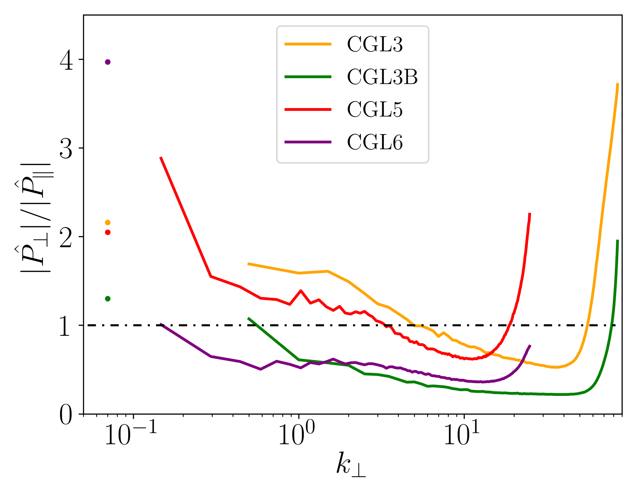
Figure 10: Ratio of the spectral distributions of the perpendicular and parallel pressures in the transverse Fourier plane, $|{\hat{P}}_{\perp}|/|{\hat{P}}_{\|}|$, where ${\displaystyle|{\hat{P}}_{\perp}|=\sqrt{\sum_{k_{\|}}\sum_{k_{\perp}\leq|{\boldsymbol{k}}^{\prime}_{\perp}|\leq k_{\perp}+\Delta k_{\perp}}|{\widehat{p}}_{\perp}({\boldsymbol{k}}^{\prime}_{\perp},k_{\|})|^{2}}}$ and ${\displaystyle|{\hat{P}}_{\|}|=\sqrt{\sum_{k_{\|}}\sum_{k_{\perp}\leq|{\boldsymbol{k}}^{\prime}_{\perp}|\leq k_{\perp}+\Delta k_{\perp}}|{\widehat{p}}_{\|}({\boldsymbol{k}}^{\prime}_{\perp},k_{\|})|^{2}}}$, plotted as a function of $k_{\perp}$, for runs CGL3 (yellow), CGL3B (green), CGL5 (red) and CGL6 (purple). Here, ${\widehat{p}}_{\perp}$ and ${\widehat{p}}_{\|}$ hold for the Fourier transform of the perpendicular and parallel pressures $p_{\perp}$ and $p_{\|}$, respectively. For comparison, the colored points on the left part of the figure indicates the ratio of the mean perpendicular and parallel pressures for the corresponding simulations.

We observe a change of pressure anisotropy, from $|{\hat{P}}_{\perp}(k_{\perp})|>|{\hat{P}}_{\|}(k_{\perp})|$ (see definitions in the figure caption) to the opposite ordering, for runs CGL3 and CGL5 at $k_{\perp}d_{i}\sim 4$. Differently, CGL3B and CGL6 show a monotonic behavior ($|{\hat{P}}_{\perp}(k_{\perp})|<|{\hat{P}}_{\|}(k_{\perp})|$) at nearly all scales (excluding the dissipation range), with the strongest pressure anisotropy at the smallest scales. We acknowledge the difficulty of relating the behavior of this quantity to the complex nonlinear terms of the exact law that involve pressure anisotropy. Nevertheless, we can speculate that the strong and uniform-in-scale pressure anisotropy observed for runs CGL3B and CGL6 would explain (or at least, is consistent with) the enhanced contribution of $\varepsilon_{\overline{\boldsymbol{\Pi}}}$ observed in the inertial range for those runs in comparison to the others. On the other hand, the change from a perpendicular-pressure dominated regime to a parallel-pressure dominated one observed for runs CGL3 and CGL5, with potential fluctuations in sign of $\Delta p$, may result in contributions that would statistically cancel out, hence the weak contribution of the anisotropic terms in the exact law for those runs.

V.2 Plasma-state distribution in the $(a_{p},\beta_{\|})$-plane

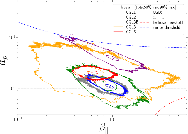
Figure 11: Distribution of the plasma states in the $(a_{p},\beta_{\parallel})$-plane with their occurrence rate : occurrence points (edge of the distribution), $50\%$ (inner ellipse) and $99\%$ (outer curves points) in the various simulations. Dash-dotted lines indicates the firehose (orange) and mirror (blue) linear instability thresholds (taking into account the isothermal electron pressure).

Name	CGL1	CGL2	CGL3	CGL3B	CGL5	CGL6
$\left<\rho\right>\pm\sigma_{\rho}$	$1.00\pm 0.02$	$1.00\pm 0.02$	$1.00\pm 0.08$	$1.00\pm 0.04$	$1.00\pm 0.02$	$1.00\pm 0.03$
$\left<\beta_{i}\right>\pm\sigma_{\beta_{i}}$	$0.99\pm 0.07$	$0.99\pm 0.06$	$1.13\pm 0.39$	$1.03\pm 0.19$	$1.07\pm 0.12$	$2.98\pm 0.25$
$\left<\beta_{\parallel}\right>\pm\sigma_{\beta_{\parallel}}$	$0.93\pm 0.09$	$0.93\pm 0.08$	$0.65\pm 0.25$	$0.87\pm 0.18$	$0.63\pm 0.07$	$1.01\pm 0.15$
$\left<a_{p}\right>\pm\sigma_{a_{p}}$	$1.11\pm 0.08$	$1.11\pm 0.10$	$2.16\pm 0.49$	$1.30\pm 0.30$	$2.05\pm 0.12$	$3.97\pm 0.47$
$a_{p}>1$(in %)	91	88	99.8	83	100	100
$a_{p}<1$(in %)	9	12	0.2	17	0	0
$\left<-\beta_{\parallel}^{*}\right>\pm\sigma_{\beta_{\parallel}^{*}}$	$0.09\pm 0.07$	$0.09\pm 0.08$	$0.71\pm 0.32$	$0.24\pm 0.24$	$0.66\pm 0.10$	$2.96\pm 0.25$

Table 2: Average and standard deviation of density $\rho$ (or electron pressure), total ionic beta-parameter $\beta_{i}=(2p_{\perp}+p_{\parallel})/(3p_{m})$ and parallel beta-parameter $\beta_{\parallel}=p_{\parallel}/p_{m}$, pressure anisotropy $a_{p}$, percentage of data points where $a_{p}>1$ or $a_{p}<1$, and parameter $-\beta_{\parallel}^{*}=\beta_{\parallel}(a_{p}-1)$, entering the terms of $\varepsilon_{\overline{\boldsymbol{\Pi}}}$ (see (5))

.

The distributions of the plasma representative points in the $(a_{p},\beta_{\parallel})$ diagram is displayed in Fig. 11, along with the thresholds of the linear firehose and mirror instabilities (see Appendix A). For all the runs, we observe that the representative points are localized in the stable region, except for a few points from CGL6 laying near the mirror-instability threshold. One can notice that the distributions associated with CGL1 to CGL5 are not centred around the initial values $a_{p0}=1$ and $\beta_{\parallel 0}=1$, but are shifted to a new regime of parameters. The representative points from simulations CGL1, CGL2 and CGL3B stay close to $a_{p0}=1$, while those corresponding to CGL3 and CGL5 shift up to an average value $\left<a_{p}\right>=2$, with however a larger standard deviation for the former run as shown in Table 2. This migration is probably due to a direct conversion at large scales of part of the injected energy into internal energy, thus enhancing the average temperatures without contributing to $\varepsilon_{iso}$, as shown by Ferrand et al. [39] with CGL1, CGL2 and CGL3 simulations. The difference in the migration appears to be consistent with the results reported above about the importance of the contribution of $\varepsilon_{\overline{\boldsymbol{\Pi}}}$ to the total cascade rate $\varepsilon_{cgl}$ at large scales where the contribution of $\left\langle\frac{\Delta p}{\rho}\right\rangle$ is dominant. However, the proportion of points with $a_{p}<1$, higher for CGL1, CGL2 and CGL3B, could explain the change of sign of $\varepsilon_{\overline{\boldsymbol{\Pi}}}$, as relatively more points with $\frac{\Delta p}{\rho}<0$ contribute to $\mathcal{S}_{\Pi 1}-\mathcal{S}_{\Pi 1}^{\langle\frac{\Delta p}{\rho}\rangle}$.

VI Conclusion

This paper summarizes the results of a study of the impact of pressure anisotropy on the turbulent cascade rate described by the exact law obtained in Simon and Sahraoui [1], using six simulations of CGL-Hall-MHD turbulence. The contribution to the exact law of the terms independent of the anisotropic component of the pressure tensor have been found to agree with the results of previous studies using incompressible or weakly compressible models with isotropic pressure. In addition, the contribution of the anisotropic component of the pressure tensor reveals

• the relevance of this effect even in a quasi-incompressible case,

• an impact of the fluctuations of pressure anisotropy (visible both in real and Fourier space) on the cascade rate in the inertial range,

• a more important effect close to the forcing scales, linked to the anisotropy of the mean pressure,

• a sign variation of the contribution of $\varepsilon_{\overline{\boldsymbol{\Pi}}}$ to the cascade rate, potentially linked to the localization of the simulation in the $(\beta_{\parallel},a_{p})$ diagram.

Even if CGL6, which is initialized with ${a_{p}}_{0}=4$, show a more prominent contribution of the pressure anisotropy term, the impact in the inertial range remains moderate. Extension of this study would require other simulations with different ${a_{p}}$ and possibly higher compressibility. Also, the exact law of Simon and Sahraoui [1] is derived with a particular form of correlation function $\mathcal{R}$. This choice is not unique, and alternative quantities have been considered in the literature [35, 27]. The sensitivity of the present conclusions to the retained correlation function is to be analyzed in further studies.

On the other hand, spacecraft data can also be used to conduct further studies, as they give access to a broad range of parameter space $(\beta_{\parallel},a_{p},\delta\rho/\rho)$. However, computing pointwise (spatial) derivatives involved in the exact law using multi-spacecraft data (e.g., Cluster or MMS) requires some caution as the uncertainties can be too large to allow a reliable quantification of the small contributions due to density fluctuations or pressure anisotropy. The nine probes of the upcoming NASA/Helioswarm mission is likely to permit improving those estimates.

VII Contribution and acknowledgement

P.S. is funded by a DIM-ACAV + Doctoral fellowship (2020-2023). She performed the present study. FS and SG supervised the work. The numerical simulation setups were designed and data were obtained within a collaboration with D. Laveder, T. Passot and P.L. Sulem who provided also figures 1 and 10. All authors contributed to discussing the results and writing the paper. PS thanks A. Jeandet for his help in the data post-processing. Computations were performed at the mesocenter Cholesky of Ecole polytechnique and mesocentre SIGAMM, hosted by Observatoire de la Côte d’Azur (OCA).

Appendix A CGL firehose and mirror instability thresholds in the presence of isothermal electrons

To obtain the CGL-MHD-instability thresholds with isothermal electrons for the firehose and mirror instabilities, we linearize the dimensionless system (1), taking $d_{i}=0$ (no Hall effect) and neglecting dissipative and forcing terms. The mean component of each quantity is isolated and indexed by the subscript $0$. Furthermore, at equilibrium, $\mathbf{v}_{0}=0$ and $\mathbf{B_{0}}=[0,0,B_{0}]_{x,y,z}$ are assumed. The electronic pressure is supposed isothermal ($\propto\rho$), consistent with the numerical simulations. Then, we apply the transformation to the Fourier space ($\partial_{t}\rightarrow-i\omega$, $\partial_{x}\rightarrow ik_{\perp}$, $\partial_{y}\rightarrow ik_{y}$, $\partial_{z}\rightarrow ik_{\parallel}$) with $k_{y}=0$. The velocity equations become

$$\left\{\begin{split}0&=-\frac{1}{v^{2}_{A0}}\omega v_{x}+\frac{\beta_{\parallel}}{2}a_{p}k_{\perp}\frac{p_{\perp}}{p_{\perp 0}}+(\frac{\beta_{\parallel}}{2}(1-a_{p})-1)k_{\parallel}\frac{B_{x}}{B_{0}}+k_{\perp}\frac{B_{z}}{B_{0}}+\frac{\beta_{e}}{2}k_{\perp}\frac{p_{e}}{p_{e0}}\\ 0&=-\frac{1}{v^{2}_{A0}}\omega v_{y}+(\frac{\beta_{\parallel}}{2}(1-a_{p})-1)k_{\parallel}\frac{B_{y}}{B_{0}}\\ 0&=-\frac{1}{v^{2}_{A0}}\omega v_{z}+\frac{\beta_{\parallel}}{2}k_{\parallel}\frac{p_{\parallel}}{p_{\parallel 0}}+\frac{\beta_{\parallel}}{2}(1-a_{p})k_{\perp}\frac{B_{x}}{B_{0}}+\frac{\beta_{e}}{2}k_{\parallel}\frac{p_{e}}{p_{e0}}\end{split}\right.$$ (11)

with $v^{2}_{A0}=\frac{B^{2}_{0}}{4\pi\rho_{0}}$, $\beta_{\parallel}=\beta_{0}\frac{4\pi p_{\parallel 0}}{B^{2}_{0}}$ and $a_{p}=\frac{p_{\perp 0}}{p_{\parallel 0}}$, $D_{i}=\frac{d_{i}}{\rho_{0}}$, $\beta_{e}=\beta_{0}\frac{4\pi p_{e0}}{B^{2}_{0}}$.

The other equations read

$$\left\{\begin{split}0&=-\omega\rho+\rho_{0}(k_{\perp}v_{x}+k_{\parallel}v_{z})\\ 0&=-\omega B_{x}-B_{0}k_{\parallel}v_{x}\\ 0&=-\omega B_{y}-B_{0}k_{\parallel}v_{y}\\ 0&=-\omega B_{z}+B_{0}k_{\perp}v_{x}\end{split}\right.$$

$$\left\{\begin{split}0&=-\omega p_{\parallel}+p_{\parallel 0}(k_{\perp}v_{x}+3k_{\parallel}v_{z})\\ 0&=-\omega p_{\perp}+p_{\perp 0}(2k_{\perp}v_{x}+k_{\parallel}v_{z})\\ 0&=-\omega p_{e}+p_{e0}(k_{\perp}v_{x}+k_{\parallel}v_{z})\end{split}\right.$$

(12)

Injecting (12) in (11) gives

$$\left\{\begin{split}0&=(-\frac{1~}{v^{2}_{A0}}\omega^{2}+(2\frac{\beta_{\parallel}}{2}a_{p}+1+\frac{\beta_{e}}{2})k^{2}_{\perp}-(\frac{\beta_{\parallel}}{2}(1-a_{p})-1)k^{2}_{\parallel})v_{x}+(\frac{\beta_{\parallel}}{2}a_{p}+\frac{\beta_{e}}{2})k_{\perp}k_{\parallel}v_{z}\\ 0&=(-\frac{1}{v^{2}_{A0}}\omega^{2}-(\frac{\beta_{\parallel}}{2}(1-a_{p})-1)k^{2}_{\parallel})v_{y}\\ 0&=(\frac{\beta_{\parallel}}{2}a_{p}+\frac{\beta_{e}}{2})k_{\perp}k_{\parallel}v_{x}+(-\frac{1}{v^{2}_{A0}}\omega^{2}+(3\frac{\beta_{\parallel}}{2}+\frac{\beta_{e}}{2})k^{2}_{\parallel})v_{z}\end{split}\right.$$ (13)

The determinant of the system (13) involves two factors. The first one gives the dispersive relation of the incompressible Alfvén-wave, polarized such as $v_{x}=v_{z}=0$ i.e. $\omega=\pm k_{\parallel}v_{A0}\sqrt{1-(\frac{\beta_{\parallel}}{2}(1-a_{p}))}$. The Alfvén wave is affected by the firehose instability that appears if

$$1-(\frac{\beta_{\parallel}}{2}(1-a_{p}))<0.$$

The second factor gives the dispersive relation of the magnetosonic waves polarized such as $v_{y}=0$, and takes the form of a second order polynomial $\omega^{4}+A_{1}\omega^{2}+A_{0}=0$ with

$$A_{1}=-v^{2}_{A0}((2\frac{\beta_{\parallel}}{2}a_{p}+1+\frac{\beta_{e}}{2})k^{2}_{\perp}+(\frac{\beta_{\parallel}}{2}(2+a_{p})+1+\frac{\beta_{e}}{2})k^{2}_{\parallel})$$

$$A_{0}=v^{2}_{A0}k^{2}_{\parallel}((\frac{\beta_{\parallel}}{2}(\frac{\beta_{\parallel}}{2}a_{p}(6-a_{p})+3)+\frac{\beta_{e}}{2}(3\frac{\beta_{\parallel}}{2}+1))k^{2}_{\perp}-(3\frac{\beta_{\parallel}}{2}+\frac{\beta_{e}}{2})(\frac{\beta_{\parallel}}{2}(1-a_{p})-1)k^{2}_{\parallel}).$$

Assuming that $k_{\perp}\gg k_{\parallel}$, $A_{0}$ gives the mirror threshold altered by the isothermal electronic pressure:

$$\frac{\beta_{\parallel}}{2}a_{p}(6-a_{p})+3+\frac{\beta_{e}}{\beta_{\parallel}}(3\frac{\beta_{\parallel}}{2}+1)=0$$

If $\beta_{e}=0$, the threshold for the CGL-MHD [44] is recovered. In our simulations, $\beta_{e}=1$.

References

- Simon and Sahraoui [2022] P. Simon and F. Sahraoui, Exact law for compressible pressure-anisotropic magnetohydrodynamic turbulence: toward linking energy cascade and instabilities, Physical Review E 105, 055111 (2022), publisher: American Physical Society.
- von Kármán and Howarth [1938] T. von Kármán and L. Howarth, On the statistical theory of isotropic turbulence, Proceedings of the Royal Society of London. Series A - Mathematical and Physical Sciences 164, 192 (1938).
- Kolmogorov [1941] A. Kolmogorov, Dissipation of energy in locally isotropic turbulence, Doklady Akademii nauk SSSR 32, 16 (1941).
- Politano and Pouquet [1998a] H. Politano and A. Pouquet, Dynamical length scales for turbulent magnetized flows, Geophysical Research Letters 25, 273 (1998a).
- Politano and Pouquet [1998b] H. Politano and A. Pouquet, von Kármán–Howarth equation for magnetohydrodynamics and its consequences on third-order longitudinal structure and correlation functions, Physical Review E 57, R21 (1998b).
- Galtier [2008] S. Galtier, von Kármán–Howarth equations for Hall magnetohydrodynamic flows, Physical Review E 77, 015302(R) (2008).
- Banerjee and Galtier [2017] S. Banerjee and S. Galtier, An alternative formulation for exact scaling relations in hydrodynamic and magnetohydrodynamic turbulence, Journal of Physics A: Mathematical and Theoretical 50, 015501 (2017).
- Hellinger et al. [2018] P. Hellinger, A. Verdini, S. Landi, L. Franci, and L. Matteini, von Kármán–Howarth equation for Hall magnetohydrodynamics: hybrid simulations, The Astrophysical Journal 857, L19 (2018), publisher: American Astronomical Society.
- Ferrand et al. [2019] R. Ferrand, S. Galtier, F. Sahraoui, R. Meyrand, N. Andrés, and S. Banerjee, On exact laws in incompressible Hall magnetohydrodynamic turbulence, The Astrophysical Journal 881, 50 (2019).
- Andrés et al. [2016a] N. Andrés, S. Galtier, and F. Sahraoui, Exact scaling laws for helical three-dimensional two-fluid turbulent plasmas, Physical Review E 94, 063206 (2016a).
- Andrés et al. [2016b] N. Andrés, P. D. Mininni, P. Dmitruk, and D. O. Gómez, von Kármán–Howarth equation for three-dimensional two-fluid plasmas, Physical Review E 93, 063202 (2016b).
- Galtier and Banerjee [2011] S. Galtier and S. Banerjee, Exact relation for correlation functions in compressible isothermal turbulence, Physical Review Letters 107, 134501 (2011), publisher: American Physical Society.
- Banerjee and Galtier [2013] S. Banerjee and S. Galtier, Exact relation with two-point correlation functions and phenomenological approach for compressible magnetohydrodynamic turbulence, Physical Review E 87, 013019 (2013).
- Banerjee and Galtier [2014] S. Banerjee and S. Galtier, A Kolmogorov-like exact relation for compressible polytropic turbulence, Journal of Fluid Mechanics 742, 230 (2014).
- Banerjee et al. [2016] S. Banerjee, L. Z. Hadid, F. Sahraoui, and S. Galtier, Scaling of compressible magnetohydrodynamic turbulence in the fast solar wind, The Astrophysical Journal Letters 829, L27 (2016), publisher: American Astronomical Society.
- Andrés and Sahraoui [2017] N. Andrés and F. Sahraoui, Alternative derivation of exact law for compressible and isothermal magnetohydrodynamics turbulence, Physical Review E 96, 053205 (2017).
- Banerjee and Kritsuk [2017] S. Banerjee and A. G. Kritsuk, Exact relations for energy transfer in self-gravitating isothermal turbulence, Physical Review E 96, 053116 (2017).
- Andrés et al. [2018a] N. Andrés, F. Sahraoui, S. Galtier, L. Z. Hadid, P. Dmitruk, and P. D. Mininni, Energy cascade rate in isothermal compressible magnetohydrodynamic turbulence, Journal of Plasma Physics 84, 21 (2018a).
- Andrés et al. [2018b] N. Andrés, S. Galtier, and F. Sahraoui, Exact law for homogeneous compressible Hall magnetohydrodynamics turbulence, Physical Review E 97, 013204 (2018b).
- Banerjee and Kritsuk [2018] S. Banerjee and A. G. Kritsuk, Energy transfer in compressible magnetohydrodynamic turbulence for isothermal self-gravitating fluids, Physical Review E 97, 023107 (2018).
- Banerjee and Andrés [2020] S. Banerjee and N. Andrés, Scale-to-scale energy transfer rate in compressible two-fluid plasma turbulence, Physical Review E 101, 043212 (2020).
- Hellinger et al. [2020] P. Hellinger, A. Verdini, S. Landi, L. Franci, E. Papini, and L. Matteini, On cascade of kinetic energy in compressible hydrodynamic turbulence, arXiv e-prints (2020), arXiv: 2004.02726.
- Simon and Sahraoui [2021] P. Simon and F. Sahraoui, General exact law of compressible isentropic magnetohydrodynamic flows: theory and spacecraft observations in the solar wind, The Astrophysical Journal 916, 49 (2021), publisher: The American Astronomical Society.
- Soulard and Briard [2022] O. Soulard and A. Briard, Cascade of circulicity in compressible turbulence, Physical Review Fluids 7, 124604 (2022), publisher: American Physical Society.
- Hellinger et al. [2021a] P. Hellinger, E. Papini, A. Verdini, S. Landi, L. Franci, L. Matteini, and V. Montagud-Camps, Spectral transfer and Kármán-Howarth-Monin equations for compressible Hall magnetohydrodynamics, The Astrophysical Journal 917, 101 (2021a), arXiv: 2104.06851.
- Hellinger et al. [2021b] P. Hellinger, A. Verdini, S. Landi, E. Papini, L. Franci, and L. Matteini, Scale dependence and cross-scale transfer of kinetic energy in compressible hydrodynamic turbulence at moderate Reynolds numbers, Physical Review Fluids 6, 044607 (2021b), publisher: American Physical Society.
- Hellinger et al. [2022] P. Hellinger, V. Montagud-Camps, L. Franci, L. Matteini, E. Papini, A. Verdini, and S. Landi, Ion-scale transition of plasma turbulence: pressure–strain effect, The Astrophysical Journal 930, 48 (2022).
- Sorriso-Valvo et al. [2007] L. Sorriso-Valvo, R. Marino, V. Carbone, A. Noullez, F. Lepreti, P. Veltri, R. Bruno, B. Bavassano, and E. Pietropaolo, Observation of inertial energy cascade in interplanetary space plasma, Physical Review Letters 99, 115001 (2007), publisher: American Physical Society.
- Andrés et al. [2019] N. Andrés, F. Sahraoui, S. Galtier, L. Z. Hadid, R. Ferrand, and S. Y. Huang, Energy cascade rate measured in a collisionless space plasma with MMS data and compressible Hall magnetohydrodynamic turbulence theory, Physical Review Letters 123, 245101 (2019), arXiv: 1911.09749.
- Sorriso-Valvo et al. [2019] L. Sorriso-Valvo, F. Catapano, A. Retinò, O. Le Contel, D. Perrone, O. W. Roberts, J. T. Coburn, V. Panebianco, F. Valentini, S. Perri, A. Greco, F. Malara, V. Carbone, P. Veltri, O. Pezzi, F. Fraternale, F. Di Mare, R. Marino, B. Giles, T. E. Moore, C. T. Russell, R. B. Torbert, J. L. Burch, and Y. V. Khotyaintsev, Turbulence-driven ion beams in the magnetospheric Kelvin-Helmholtz instability, Physical Review Letters 122, 035102 (2019), publisher: American Physical Society.
- Hadid et al. [2017] L. Z. Hadid, F. Sahraoui, and S. Galtier, Energy cascade rate in compressible fast and slow solar wind turbulence, The Astrophysical Journal 838, 9 (2017), arXiv: 1612.02150.
- Osman et al. [2013] K.T. Osman, W. H. Matthaeus, K. H. Kiyani, B. Hnat, and S. C. Chapman, Proton kinetic effects and turbulent energy cascade rate in the solar wind, Physical Review Letters 111, 201101 (2013).
- Carbone et al. [2009] V. Carbone, R. Marino, L. Sorriso-Valvo, A. Noullez, and R. Bruno, Scaling laws of turbulence and heating of fast solar wind: the role of density fluctuations, Physical Review Letters 103, 061102 (2009), publisher: American Physical Society.
- Hadid et al. [2018] L. Z. Hadid, F. Sahraoui, S. Galtier, and S. Y. Huang, Compressible magnetohydrodynamic turbulence in the Earth’s magnetosheath: estimation of the energy cascade rate using in situ spacecraft data, Physical Review Letters 120, 055102 (2018).
- Ferrand et al. [2020] R. Ferrand, S. Galtier, F. Sahraoui, and C. Federrath, Compressible turbulence in the interstellar medium: new insights from a high-resolution supersonic turbulence simulation, The Astrophysical Journal 904, 160 (2020).
- Mininni and Pouquet [2009] P. D. Mininni and A. Pouquet, Finite dissipation and intermittency in magnetohydrodynamics, Physical Review E 80, 025401(R) (2009).
- Kritsuk et al. [2013] A. G. Kritsuk, R. Wagner, and M. L. Norman, Energy cascade and scaling in supersonic isothermal turbulence, Journal of Fluid Mechanics 729, 1 (2013).
- Ferrand et al. [2022] R. Ferrand, F. Sahraoui, S. Galtier, N. Andrés, P. Mininni, and P. Dmitruk, An in-depth numerical study of exact laws for compressible Hall magnetohydrodynamic turbulence, The Astrophysical Journal 927, 205 (2022).
- Ferrand et al. [2021] R. Ferrand, F. Sahraoui, D. Laveder, T. Passot, P. L. Sulem, and S. Galtier, Fluid energy cascade rate and kinetic damping: new insight from 3D Landau-fluid simulations, The Astrophysical Journal 923, 122 (2021), publisher: The American Astronomical Society.
- Jiang et al. [2023] B. Jiang, C. Li, Y. Yang, K. Zhou, W. H. Matthaeus, and M. Wan, Energy transfer and third-order law in forced anisotropic magneto-hydrodynamic turbulence with hyper-viscosity, Journal of Fluid Mechanics 974, A20 (2023).
- Bale et al. [2009] S. D. Bale, J. C. Kasper, G. G. Howes, E. Quataert, C. Salem, and D. Sundkvist, Magnetic fluctuation power near proton temperature anisotropy instability thresholds in the solar wind, Physical Review Letters 103, 211101 (2009).
- Hellinger et al. [2017] P. Hellinger, S. Landi, L. Matteini, A. Verdini, and L. Franci, Mirror instability in the turbulent solar wind, The Astrophysical Journal 838, 158 (2017), publisher: American Astronomical Society.
- Chew et al. [1956] G. F. Chew, M. Goldberger, and F. E. Low, The Boltzmann equation and the one-fluid hydromagnetic equations in the absence of particle collisions, Proceedings of the Royal Society of London. Series A. Mathematical and Physical Sciences 236, 112 (1956).
- Hunana et al. [2019] P. Hunana, A. Tenerani, G. P. Zank, E. Khomenko, M. L. Goldstein, G. M. Webb, P. S. Cally, M. Collados, M. Velli, and L. Adhikari, An introductory guide to fluid models with anisotropic temperatures. Part 1. CGL description and collisionless fluid hierarchy, Journal of Plasma Physics 85, 205850602 (2019).
- Hunana and Zank [2017] P. Hunana and G. P. Zank, On the parallel and oblique firehose instability in fluid models, The Astrophysical Journal 839, 13 (2017), publisher: American Astronomical Society.
- Sahraoui et al. [2003] F. Sahraoui, G. Belmont, and L. Rezeau, Hamiltonian canonical formulation of Hall-magnetohydrodynamics: toward an application to weak turbulence theory, Physics of Plasmas 10, 1325 (2003), publisher: American Institute of Physics.
- Lamriben et al. [2011] C. Lamriben, P.-P. Cortet, and F. Moisy, Direct measurements of anisotropic energy transfers in a rotating turbulence experiment, Physical Review Letters 107, 024503 (2011).
- Manzini et al. [2022] D. Manzini, F. Sahraoui, F. Califano, and R. Ferrand, Local cascade and dissipation in incompressible Hall magnetohydrodynamic turbulence: the Coarse-Graining approach, Physical Review E 106, 035202 (2022), arXiv:2203.01050 [physics].
- Cho and Lazarian [2009] J. Cho and A. Lazarian, Simulations of electron magnetohydrodynamic turbulence, The Astrophysical Journal 701, 236 (2009).