Characterizing Biphoton Spatial Wave Function Dynamics with Quantum Wavefront Sensing
Abstract
With an extremely high dimensionality, the spatial degree of freedom of entangled photons is a key tool for quantum foundation and applied quantum techniques. To fully utilize the feature, the essential task is to experimentally characterize the multiphoton spatial wave function including the entangled amplitude and phase information at different evolutionary stages. However, there is no effective method to measure it. Quantum state tomography is costly, and quantum holography requires additional references. Here we introduce quantum Shack–Hartmann wavefront sensing to perform efficient and reference-free measurement of the biphoton spatial wave function. The joint probability distribution of photon pairs at the back focal plane of a microlens array is measured and used for amplitude extraction and phase reconstruction. In the experiment, we observe that the biphoton amplitude correlation becomes weak while phase correlation shows up during free-space propagation. Our work is a crucial step in quantum physical and adaptive optics and paves the way for characterizing quantum optical fields with high-order correlations or topological patterns.
Introduction.—The photon is a promising system in fundamental quantum physics and applied quantum techniques [1]. Its spatial degree of freedom is the core of high-dimensional quantum communication and quantum imaging [2], including ghost imaging [3], imaging with undetected photons [4], image distillation [5] and super-resolution imaging [6, 7]. Developing experimental methods to characterize the entangled multiphoton states is a basic task [8]. For the spatial state (sometimes called the wave function [9]), direct coincidence counting can only reveal the joint probability distribution (JPD), i.e., the squared modulus of the wave function [10], while effective phase measurement methods will become useful in various applications like information encoding [11], biomedical phase imaging [12], and aberration cancellation. Moreover, photons are prone to various evolution and modulation processes, so observing the state dynamics is even more exciting and challenging.
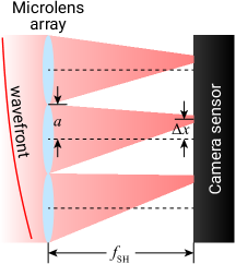
Researches on biphoton phase measurement can be inspired by classical methods. A prominent type is holography [13], which needs a reference beam for interference. It has the highest accuracy and is very suitable for characterizing transparent objects. In quantum optics, polarization entanglement enables phase-shifting holography [14, 15, 16], and biphoton interference has been employed to measure the biphoton spatial wave function [17]. However, the reference beam may contain aberrations, and is not always available. Starting from Zernike’s phase contrast microscopy [18], one type of reference-free methods is selecting a part of the unknown field as the reference, including some weak measurement methods [19, 9, 20]. Our group used the setup devised by Kocsis et al. [21] to obtain the phase gradient distribution [22] for phase reconstruction [23, 24], and named it the weak measurement wavefront sensor [25, 26]. Like some shearing methods, it is an interference of the original beam with a slightly displaced one. Then, our group extended it to the multiphoton case [27], which requires JPD measurement of photons. However, weak measurement methods require a high signal-to-noise ratio, which is difficult for biphoton fields in experiments. There are other methods which do not need any reference. State tomography [28] requiring a huge number of projection bases is possible but impractical. Here, we consider the celebrated Shack–Hartmann wavefront sensing (SHWS) [29], which uses a microlens array to project the phase gradient at each aperture to the displacement of the focused spot [30, 25]. The Supplemental Material (SM) [31] introduces basic concepts of SHWS.
In this proof-of-principle work, we introduce and implement quantum SHWS (QSHWS) by measuring the JPD of photon pairs from spontaneous parametric down-conversion (SPDC) [32, 33] at the focal plane of the microlens array. To our knowledge, this is the first single-measurement and reference-free biphoton phase measurement method. As for the JPD measurement, traditional scanning and coincidence counting method [10] is time-consuming. In 2018, Defienne et al. demonstrated that it can be calculated from multiple frames taken by an electron-multiplying charge-coupled device (EMCCD) or single-photon avalanche photodiode (SPAD) array camera [34, 35, 36], which we refer to as the multiple frame method. Then, we focus on the biphoton propagation dynamics as an example. Chan et al. [37] derived that SPDC photon pairs would be less correlated in position after free-space propagation [38] while phase correlation shows up. We use QSHWS to measure the biphoton state after free-space propagation, and show they agree with theoretical predictions using double-Gaussian approximation [39, 37, 40, 33]. Furthermore, we use a spatial light modulator (SLM) to encode a hyperbolic paraboloid (saddle) phase pattern for detection. Finally, we describe potential applications of QSHWS in biphoton physical [41] and adaptive optics [42, 43].
Theory.—We consider photon pairs with a definite polarization and wavelength. Denoting the spatial wave function as and its phase , when the post-selected position of photon 1 takes all the values inside a microlens aperture , the conditional state of photon 2 is generally mixed, described by the reduced density matrix and its function in the position basis (corresponding to the mutual coherence function [44, 45, 46, 25]). If a single-photon pure state is used, from the spot centroid displacement from the center of another aperture at the camera, the phase gradient at is calculated by , where is the microlens focal length. However, using the mixed state , the measured phase gradient becomes [25, 47] (See SM [31] for a full derivation)
| (1) |
When the aperture is sufficiently small, can be approximated by points , and Eq. (Characterizing Biphoton Spatial Wave Function Dynamics with Quantum Wavefront Sensing) becomes the partial phase gradient . Exchanging and yields another partial gradient . The joint phase can be reconstructed by line integral [27]
| (2) |
For the amplitude part, with the measured JPD at the microlens focal plane, assuming each microlens is lossless and its incoming beam does not escape its aperture, the JPD of two apertures (Here are centered by respectively), which equals . The reconstructed wave function is thus .
If the two photons are indistinguishable , only one phase gradient distribution can be measured. Without loss of generality, let it be , then , and the reconstructed has exchange symmetry.
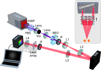
Experimental setup.—The experimental setup is shown in Fig. 1. A pump laser at is incident on a -barium borate (BBO) crystal. Degenerate near-collinear type-I SPDC photon pairs pass through two Fourier lenses, get reflected by a SLM, pass through another Fourier lens and arrive at the microlens array. The width of each microlens is . An imaging lens is inserted at the midpoint of the microlens array and the EMCCD sensor. See SM [31] for details.
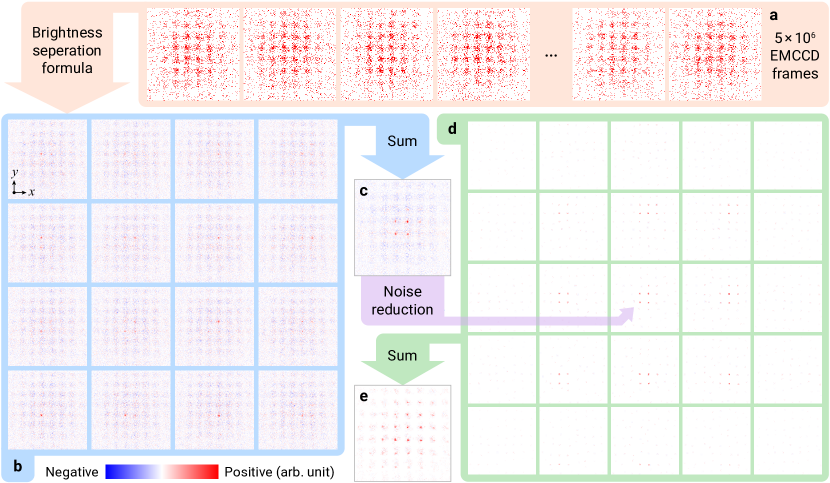
Data processing.—In one measurement, the EMCCD takes multiple frames, and a threshold determines whether pixels of each frame have at least one photon. In the multiple frame method, the JPD is calculated by the covariance of the counts at two pixels, which, however, only suits for biphoton with a strong position correlation and thus narrow conditional probability distributions (CPDs, with the position of one photon given) due to its signal-to-noise ratio [35, 38]. Also, photon intensity or sensor efficiency fluctuation results in a positive background in the calculated JPD, so a successive frame formula is mainly used in subsequent works [5, 15, 43], which will cause more noise in the JPD [7], and the background removal is not effective in our experiments. We develop a brightness separation formula where frames registering too many or few photons are discarded, and the background is basically eliminated.
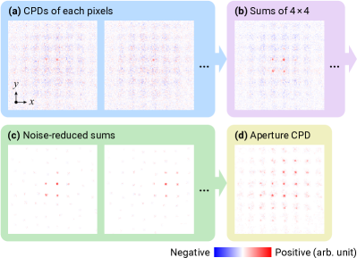
Single-pixel CPDs of pixels within an aperture are summed to obtain the aperture CPD, but direct summation will distort the result. We choose to divide the aperture into several -pixel segments, sum CPDs over each segment first, and reduce the noise before being summed for the final aperture CPD. Fig. 2 illustrates the processes. Finally, the centroid positions of the spots are calculated from the aperture CPD and converted to the phase gradient distribution.
An algorithm is required to realize the phase reconstruction in Eq. (2). For the four-dimensional phase distribution, traditional zonal and modal method [24] which require large matrix operations is difficult to implement. We adapt the method based on random point spreading and averaging in Ref. [27]. SM [31] provides all details of data processing.
Biphoton propagation dynamics.—Using the microlens array, the biphoton position anti-correlation after three Fourier lenses with the SLM off can be observed easily, as shown in Fig. 3(a). The anti-correlation is not aperture-to-aperture because its center is not a grid point of the microlens array.
However, the phase cannot be reconstructed without magnification for biphoton states with strong position correlation (See Discussion). To demonstrate the phase measurement, we need states with wider CPDs. Due to the immaturity of arbitrary two-photon interaction and modulation, more general correlated phase patterns cannot be generated experimentally. We choose to measure the correlated phase of propagated SPDC photon pairs. Before propagation, their wave function can be approximated by a double-Gaussian function (unnormalized) [39, 37, 40, 33]
| (3) |
In the momentum space (angular spectrum [48]), it is the Fourier transform of Eq. (3),
| (4) |
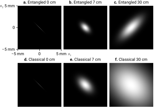
After propagating a distance , a phase is added to the angular spectrum and thus , where and . Substituting the new complex into Eq. (3) yields the new wave function with phase correlation. When , the photons have no amplitude correlation, and entanglement only exists in the phase [37]. The amplitude correlation direction switches when .
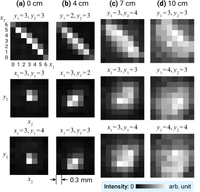
Previously, the biphoton JPD at intermediate distances cannot be measured using the multiple frame method [38]. Now, we reconstruct the wave functions of SPDC photon pairs propagating , , and . Data of farther distances are still limited by the signal-to-noise ratio. The position correlation patterns and selected CPDs are shown in Figs. 3(b)–(d), where the anti-correlation becomes weaker and CPDs become wider as increases.
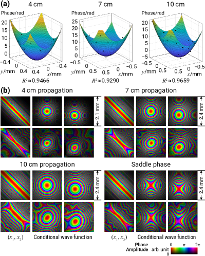
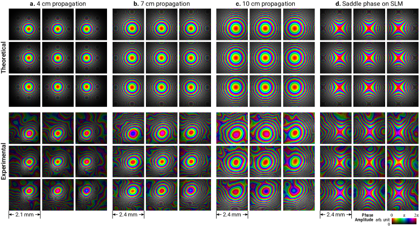
The theoretical phases of conditional wave functions are approximately spherical waves at twice the actual propagation distances, which can be explained in the next section. First, we do not interpolate the phase gradient distribution, and the reconstructed phase of conditional wave functions at a near-center aperture are fitted by phases of spherical waves at distances , and with displacements to be determined as shown in Fig. 4(a). The coefficients of determination () characterizing the similarity are also given, showing the reconstructed phases fit well with theory where the JPD values are higher (otherwise the noise in the aperture CPDs distorts the phase gradient). As the phase of the wave function are quadratic, its gradients are linear functions of the coordinates, valid for linear interpolation.
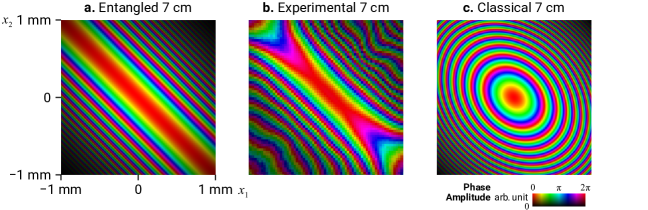
Then, we reconstruct wave functions from the interpolated ( times) JPDs of two apertures and gradient distributions. Selected slices of them are shown in Fig. 4(b), where the theoretical counterparts from Eq. (3) are also plotted (, . See SM [31] for the calculation, which includes Ref. [49] about the refractive indices of BBO). Without interpolation, the phase patterns may be difficult to recognize from phase values modulo . In the conditional wave functions, the center of the paraboloid phase pattern is anti-correlated with the given point. In regions where JPD values are higher, the reconstructed wave functions fit well with the theory. If these wave functions are Fourier transformed, the positive momentum correlation and the global paraboloid phase can be observed, as shown in SM [31].
Note that classically correlated photon pair has almost no momentum correlation, so measuring the JPD in the momentum space can tell whether they are entangled [10, 50]. In SM [31], we give a form of mixed two-photon state with position anti-correlation, briefly analyze its propagation and the measured values, compared with the entangled state above.
Phase modulation.—If a phase pattern is added on the SLM, the biphoton wave function at the SLM is multiplied by . Letting the Fourier transform of be , where is the focal length of the third Fourier lens, the wave function at the microlens array becomes . Assuming the photon pairs are originally perfectly anti-correlated , it is
| (5) |
where the convolution only performs on (See SM [31] for its derivation). If (the anti-correlated Einstein–Podolsky–Rosen state [51]), the conditional wave function with a given is , which is the Fourier transform of displaced by .
Adding a paraboloid phase on the SLM can simulate the propagation of . The Fourier transform of is a spherical wave at in classical optics, and thus the conditional wave functions take this form. If a saddle phase is added, it propagates forward in the direction and backward in , resulting in the saddle phase in the conditional wave functions. We choose the forward and backward distance to be cm. In the reconstructed phase as shown in Fig. 4(b), the magnitudes at the and direction are slightly different, which is possibly caused by a slight wavefront curvature of the pump beam, the obliquity of the SLM, or the deviation of the imaging lens magnification factor from . As the latter two can be eliminated, this method may be used to detect low-order global phase of photon pairs correlated in position, which is hard to measure without propagation.
Discussion.—In this work, we introduced the quantum Shack–Hartmann wavefront sensing method to reconstruct the biphoton spatial wave function, developed the data processing algorithms, and performed the experiments of biphoton propagation dynamics and saddle phase modulation. This method only requires one measurement and is reference-free, but the spatial resolution is the major shortcoming. Amplitude and phase patterns with higher spatial complexities cannot be detected without magnification. Although the CPD width limit in the multiple frame method is greatly lowered with the microlens array, the signal-to-noise ratio still hinders the detection of far wider CPDs, which may be overcome by a time-stamping camera like Tpx3Cam [50, 17]. Recently, another wavefront sensor based on spatial masking and diffraction with a high resolution was invented [52], which may be considered in quantum wavefront sensing in the future.
Classical SHWS has been widely used in fields like astronomy, laser optics and biomedical imaging, while QSHWS can be applied in various tasks in the emerging field of adaptive quantum optics [42, 43]. The phase information that lies in the second-order correlation can be assisted in astronomical observation, multiphoton physical optics [41] and free-space quantum communication against atmospheric turbulence. When studying multiphoton interaction or modulation media like nonlinear crystals and atom ensembles [53], the correlated phase aberration cannot be measured classically, while QSHWS may be the solution.
Theoretically, the single-pixel CPD shown in Fig. 2(a) provides more information of the biphoton field, linking the combination of the position and phase gradient of one photon to that of the other. For example, it reveals some properties of mixed states [44, 45], and might be used for information encoding and secret sharing. Although the photon pairs are indistinguishable in our experiments, they can be spatially separated or have different wavelengths. This method is not limited to two photons [27]. If the JPD of more photons can be measured, the multiphoton wave function can also be reconstructed, leading to the measurement of higher-order correlations. Finally, this wavefront sensing technique can also be used in other continuous-variable degrees of freedom, such as frequency, by converting them into spatial entanglement [54, 55], as well as combining topology and entanglement [56] in quantum optics.
Acknowledgements.
This work was supported by the Innovation Program for Quantum Science and Technology (No. 2021ZD0301200, No. 2021ZD0301400), National Natural Science Foundation of China (No. 62005263, No. 11821404, No. U19A2075, No. 92365205), Anhui Initiative in Quantum Information Technologies (No. AHY060300), the Fundamental Research Funds for the Central Universities (No. WK2030000069), the China Postdoctoral Science Foundation (No. 478 2020M671862). Y.Z. and Z.-D.L. contributed equally to this work.References
- Flamini et al. [2018] F. Flamini, N. Spagnolo, and F. Sciarrino, Photonic quantum information processing: a review, Rep. Prog. Phys. 82, 016001 (2018).
- Magaña-Loaiza and Boyd [2019] O. S. Magaña-Loaiza and R. W. Boyd, Quantum imaging and information, Rep. Prog. Phys. 82, 124401 (2019).
- Pittman et al. [1995] T. B. Pittman, Y. H. Shih, D. V. Strekalov, and A. V. Sergienko, Optical imaging by means of two-photon quantum entanglement, Phys. Rev. A 52, R3429 (1995).
- Lemos et al. [2014] G. B. Lemos, V. Borish, G. D. Cole, S. Ramelow, R. Lapkiewicz, and A. Zeilinger, Quantum imaging with undetected photons, Nature (London) 512, 409 (2014).
- Defienne et al. [2019] H. Defienne, M. Reichert, J. W. Fleischer, and D. Faccio, Quantum image distillation, Sci. Adv. 5, eaax0307 (2019).
- Giovannetti et al. [2009] V. Giovannetti, S. Lloyd, L. Maccone, and J. H. Shapiro, Sub-Rayleigh-diffraction-bound quantum imaging, Phys. Rev. A 79, 013827 (2009).
- He et al. [2023] Z. He, Y. Zhang, X. Tong, L. Li, and L. V. Wang, Quantum microscopy of cells at the Heisenberg limit, Nat. Commun. 14, 2441 (2023).
- Pan et al. [2019] W.-W. Pan, X.-Y. Xu, Y. Kedem, Q.-Q. Wang, Z. Chen, M. Jan, K. Sun, J.-S. Xu, Y.-J. Han, C.-F. Li, and G.-C. Guo, Direct Measurement of a Nonlocal Entangled Quantum State, Phys. Rev. Lett. 123, 150402 (2019).
- Lundeen et al. [2011] J. S. Lundeen, B. Sutherland, A. Patel, C. Stewart, and C. Bamber, Direct measurement of the quantum wavefunction, Nature (London) 474, 188 (2011).
- Howell et al. [2004] J. C. Howell, R. S. Bennink, S. J. Bentley, and R. W. Boyd, Realization of the Einstein-Podolsky-Rosen Paradox Using Momentum- and Position-Entangled Photons from Spontaneous Parametric Down Conversion, Phys. Rev. Lett. 92, 210403 (2004).
- Wang et al. [2012] J. Wang, J.-Y. Yang, I. M. Fazal, N. Ahmed, Y. Yan, H. Huang, Y. Ren, Y. Yue, S. Dolinar, M. Tur, and A. E. Willner, Terabit free-space data transmission employing orbital angular momentum multiplexing, Nat. Photon. 6, 488 (2012).
- Park et al. [2018] Y. Park, C. Depeursinge, and G. Popescu, Quantitative phase imaging in biomedicine, Nat. Photon. 12, 578 (2018).
- Gabor [1948] D. Gabor, A New Microscopic Principle, Nature (London) 161, 777 (1948).
- Yamaguchi and Zhang [1997] I. Yamaguchi and T. Zhang, Phase-shifting digital holography, Opt. Lett. 22, 1268 (1997).
- Defienne et al. [2021] H. Defienne, B. Ndagano, A. Lyons, and D. Faccio, Polarization entanglement-enabled quantum holography, Nat. Phys. 17, 591 (2021).
- Camphausen et al. [2021] R. Camphausen, Álvaro Cuevas, L. Duempelmann, R. A. Terborg, E. Wajs, S. Tisa, A. Ruggeri, I. Cusini, F. Steinlechner, and V. Pruneri, A quantum-enhanced wide-field phase imager, Sci. Adv. 7, eabj2155 (2021).
- Zia et al. [2023] D. Zia, N. Dehghan, A. D’Errico, F. Sciarrino, and E. Karimi, Interferometric imaging of amplitude and phase of spatial biphoton states, Nat. Photon. 17, 1009 (2023).
- Zernike [1955] F. Zernike, How I Discovered Phase Contrast, Science 121, 345 (1955).
- Dressel et al. [2014] J. Dressel, M. Malik, F. M. Miatto, A. N. Jordan, and R. W. Boyd, Colloquium: Understanding quantum weak values: Basics and applications, Rev. Mod. Phys. 86, 307 (2014).
- Shi et al. [2015] Z. Shi, M. Mirhosseini, J. Margiewicz, M. Malik, F. Rivera, Z. Zhu, and R. W. Boyd, Scan-free direct measurement of an extremely high-dimensional photonic state, Optica 2, 388 (2015).
- Kocsis et al. [2011] S. Kocsis, B. Braverman, S. Ravets, M. J. Stevens, R. P. Mirin, L. K. Shalm, and A. M. Steinberg, Observing the Average Trajectories of Single Photons in a Two-Slit Interferometer, Science 332, 1170 (2011).
- Yang et al. [2020] M. Yang, Y. Xiao, Y.-W. Liao, Z.-H. Liu, X.-Y. Xu, J.-S. Xu, C.-F. Li, and G.-C. Guo, Zonal Reconstruction of Photonic Wavefunction via Momentum Weak Measurement, Laser Photon. Rev. 14, 1900251 (2020).
- Hudgin [1977] R. H. Hudgin, Wave-front reconstruction for compensated imaging, J. Opt. Soc. Am. 67, 375 (1977).
- Southwell [1980] W. Southwell, Wave-front estimation from wave-front slope measurements, J. Opt. Soc. Am. 70, 998 (1980).
- Zheng et al. [2021] Y. Zheng, M. Yang, Z.-H. Liu, J.-S. Xu, C.-F. Li, and G.-C. Guo, Detecting momentum weak value: Shack–Hartmann versus a weak measurement wavefront sensor, Opt. Lett. 46, 5352 (2021).
- Zheng et al. [2022] Y. Zheng, M. Yang, Z.-H. Liu, J.-S. Xu, C.-F. Li, and G.-C. Guo, Toward practical weak measurement wavefront sensing: spatial resolution and achromatism, Opt. Lett. 47, 2734 (2022).
- Zheng et al. [2023] Y. Zheng, M. Yang, Y.-W. Liao, J.-S. Xu, C.-F. Li, and G.-C. Guo, Reconstructing the multiphoton spatial wave function with coincidence wave-front sensing, Phys. Rev. A 107, 042608 (2023).
- Hu et al. [2020] X.-M. Hu, W.-B. Xing, B.-H. Liu, Y.-F. Huang, C.-F. Li, G.-C. Guo, P. Erker, and M. Huber, Efficient Generation of High-Dimensional Entanglement through Multipath Down-Conversion, Phys. Rev. Lett. 125, 090503 (2020).
- Platt and Shack [2001] B. C. Platt and R. Shack, History and Principles of Shack-Hartmann Wavefront Sensing, J. Refract. Surg. 17, S573 (2001).
- Ares et al. [2000] J. Ares, T. Mancebo, and S. Bará, Position and displacement sensing with Shack–Hartmann wave-front sensors, Appl. Opt. 39, 1511 (2000).
- [31] See Supplemental Material at http://link.aps.org/supplemental/ for details of the experimental setup, data processing, more figures, and theoretical analyses.
- Walborn et al. [2010] S. Walborn, C. Monken, S. Pádua, and P. Souto Ribeiro, Spatial correlations in parametric down-conversion, Phys. Rep. 495, 87 (2010).
- Schneeloch and Howell [2016] J. Schneeloch and J. C. Howell, Introduction to the transverse spatial correlations in spontaneous parametric down-conversion through the biphoton birth zone, J. Opt. 18, 053501 (2016).
- Defienne et al. [2018a] H. Defienne, M. Reichert, and J. W. Fleischer, General Model of Photon-Pair Detection with an Image Sensor, Phys. Rev. Lett. 120, 203604 (2018a).
- Reichert et al. [2018] M. Reichert, H. Defienne, and J. W. Fleischer, Optimizing the signal-to-noise ratio of biphoton distribution measurements, Phys. Rev. A 98, 013841 (2018).
- Ndagano et al. [2022] B. Ndagano, H. Defienne, D. Branford, Y. D. Shah, A. Lyons, N. Westerberg, E. M. Gauger, and D. Faccio, Quantum microscopy based on Hong–Ou–Mandel interference, Nat. Photon. 16, 384 (2022).
- Chan et al. [2007] K. W. Chan, J. P. Torres, and J. H. Eberly, Transverse entanglement migration in Hilbert space, Phys. Rev. A 75, 050101(R) (2007).
- Bhattacharjee et al. [2022] A. Bhattacharjee, M. K. Joshi, S. Karan, J. Leach, and A. K. Jha, Propagation-induced revival of entanglement in the angle-OAM bases, Sci. Adv. 8, eabn7876 (2022).
- Law and Eberly [2004] C. K. Law and J. H. Eberly, Analysis and Interpretation of High Transverse Entanglement in Optical Parametric Down Conversion, Phys. Rev. Lett. 92, 127903 (2004).
- Reichert et al. [2017] M. Reichert, X. Sun, and J. W. Fleischer, Quality of spatial entanglement propagation, Phys. Rev. A 95, 063836 (2017).
- Saleh et al. [2005] B. E. A. Saleh, M. C. Teich, and A. V. Sergienko, Wolf Equations for Two-Photon Light, Phys. Rev. Lett. 94, 223601 (2005).
- Defienne et al. [2018b] H. Defienne, M. Reichert, and J. W. Fleischer, Adaptive Quantum Optics with Spatially Entangled Photon Pairs, Phys. Rev. Lett. 121, 233601 (2018b).
- Cameron et al. [2024] P. Cameron, B. Courme, C. Vernière, R. Pandya, D. Faccio, and H. Defienne, Adaptive optical imaging with entangled photons, Science 383, 1142 (2024).
- Hradil et al. [2010] Z. Hradil, J. Řeháček, and L. L. Sánchez-Soto, Quantum Reconstruction of the Mutual Coherence Function, Phys. Rev. Lett. 105, 010401 (2010).
- Stoklasa et al. [2014] B. Stoklasa, L. Motka, J. Rehacek, Z. Hradil, and L. L. Sánchez-Soto, Wavefront sensing reveals optical coherence, Nat. Commun. 5, 3275 (2014).
- Zhou et al. [2021] Y. Zhou, J. Zhao, D. Hay, K. McGonagle, R. W. Boyd, and Z. Shi, Direct Tomography of High-Dimensional Density Matrices for General Quantum States of Photons, Phys. Rev. Lett. 127, 040402 (2021).
- [47] The symbol means taking the gradient with respect to the first vector variable. For example, .
- Goodman [2017] J. W. Goodman, Introduction to Fourier Optics, 4th ed. (W. H. Freeman, 2017).
- Eimerl et al. [1987] D. Eimerl, L. Davis, S. Velsko, E. K. Graham, and A. Zalkin, Optical, mechanical, and thermal properties of barium borate, J. Appl. Phys. 62, 1968 (1987).
- Courme et al. [2023] B. Courme, C. Vernière, P. Svihra, S. Gigan, A. Nomerotski, and H. Defienne, Quantifying high-dimensional spatial entanglement with a single-photon-sensitive time-stamping camera, Opt. Lett. 48, 3439 (2023).
- Einstein et al. [1935] A. Einstein, B. Podolsky, and N. Rosen, Can Quantum-Mechanical Description of Physical Reality Be Considered Complete?, Phys. Rev. 47, 777 (1935).
- Yi et al. [2021] S. Yi, J. Xiang, M. Zhou, Z. Wu, L. Yang, and Z. Yu, Angle-based wavefront sensing enabled by the near fields of flat optics, Nat. Commun. 12, 6002 (2021).
- Nirala et al. [2023] G. Nirala, S. T. Pradyumna, A. Kumar, and A. M. Marino, Information encoding in the spatial correlations of entangled twin beams, Sci. Adv. 9, eadf9161 (2023).
- Liu et al. [2018] Z.-D. Liu, H. Lyyra, Y.-N. Sun, B.-H. Liu, C.-F. Li, G.-C. Guo, S. Maniscalco, and J. Piilo, Experimental implementation of fully controlled dephasing dynamics and synthetic spectral densities, Nat. Commun. 9, 3453 (2018).
- Liu et al. [2020] Z.-D. Liu, Y.-N. Sun, B.-H. Liu, C.-F. Li, G.-C. Guo, S. Hamedani Raja, H. Lyyra, and J. Piilo, Experimental realization of high-fidelity teleportation via a non-Markovian open quantum system, Phys. Rev. A 102, 062208 (2020).
- Tam et al. [2022] P. M. Tam, M. Claassen, and C. L. Kane, Topological Multipartite Entanglement in a Fermi Liquid, Phys. Rev. X 12, 031022 (2022).
Characterizing Biphoton Spatial Wave Function Dynamics with Quantum Wavefront Sensing: Supplemental Material
Yi Zheng, Zhao-Di Liu, Rui-Heng Miao, Jin-Ming Cui, Mu Yang, Xiao-Ye Xu, Jin-Shi Xu, Chuan-Feng Li and Guang-Can Guo
A. Concepts of classical Shack–Hartmann wavefront sensing
Here we review the basic principle and limitations of classical SHWS. The one-dimensional case is illustrated in Fig. S1. A monochromatic light beam at with a curved wavefront is incident on the microlens array whose focal length is . On each microlens aperture with a width , the beam can be regarded as a tilted plane wave. So, measuring the centroid position of the spot at the back focal plane of a certain microlens , the tilt angle is , and the transverse component of the wave vector . Evaluating all the microlenses, we have a distribution of , denoted as the function . SHWS is insensitive to polarization, and according to dispersion, has little dependence on , which may be negligible.
Denoting the complex amplitude of the beam as and its phase , by analyzing the average angular spectrum of the optical field within one microlens aperture, letting be the center of one microlens, we have [1]
| (S1) |
which means is the weighted average of the phase derivative over the aperture according to the intensity . If the phase derivative does not change much inside each aperture, we have . Integrating yields the phase distribution we would like to measure. By summing the intensity values within each aperture one also obtains the intensity distribution , then the complex amplitude can be reconstructed . So, SHWS simultaneously measures the intensity and the phase gradient distribution at a reduced spatial resolution.
If the beam is partially coherent described by the mutual coherence function (at the same time; corresponding to the density matrix in the position basis [2]), the phase is not defined, and the measured “phase derivative” using SHWS is [2]
| (S2) |
which becomes Eq. (S1) when the field is coherent . Here means taking the partial derivative of the first variable, i.e., . When the aperture at is small, Eq. (S2) is approximated by . One can verify that when the partially coherent beam passes through a pure-phase object , its mutual coherence function becomes , and is added to the measured “phase derivative” [3]. This means one does not need perfect coherent beam to illuminate a pure-phase object in order to measure its optical path difference distribution, but the focused spot size will be larger.
Eq. (S2) can be generalized to the two-dimensional case. Let be the aperture with its center and width . First, we only consider the measured “partial derivative of phase with respect to ”, which is calculated from the coordinate of the spot centroid. The original mutual coherence function is . Ignoring the coordinate inside the aperture, the result is similar as a partial trace . Substituting it into Eq. (S2) yields
| (S3) |
Similarly, for “partial derivative of phase with respect to ”, the result is
| (S4) |
Combined as a vector, the measured “phase gradient” by SHWS at aperture from the partially coherent light is
| (S5) |
The spatial resolution determined by the microlens size is the major shortcoming of SHWS. If varies rapidly in neighboring apertures (e.g., the beam width is comparable to or smaller than the aperture), SHWS cannot correctly reconstruct the phase. If sharp changes in the measured intensity distribution, or larger and distorted focused spots inside apertures are observed, the user can know the spatial resolution is not enough, and a system should be used to magnify the beam. Also, if has zeroes (e.g. Hermite–Gaussian beams), the phase differences between different spots cannot be detected.
If the microlens size decreases, the spatial resolution is enhanced, but the light spots on the camera sensor becomes larger, which means the local momentum measurement is less certain. This exemplifies the uncertainty principle. However, for SHWS, only the average positions of the spots are used, so larger spots do not limit SHWS in principle, only affecting its efficiency. Another disadvantage is that the dynamic range will decrease, i.e., the maximally detectable tilt angle becomes small.
B. Full derivation of Eq. (1) of the main text
Using the mixed state described by the density matrix (unnormalized) at the position basis
| (S6) |
according to Eq. (S5), the measured “phase gradient” by SHWS at aperture , which is calculated from the spot centroid position, is
| (S7) |
where .
C. Details of the experimental setup
A laser with passes through a beam shaping system to ensure that the beam is roughly Gaussian, and pumps the BBO crystal with a thickness . The pump beam at the crystal has a beam radius of about mm, and is then removed by a long-pass interference filter (IF) at nm. Two Fourier lenses with cm and cm magnify the beam times to the SLM (Hamamatsu LCOS-SLM X13138-02. Pixel size: µm). The light reflected by the SLM passes through a third Fourier lens with cm and is incident on the microlens array with the lens width mm, the array period mm, the focal length mm and the total size . Since the effective clear aperture of the microlens array is mm mm, the number of effective microlenses is . As the focal length of the microlens array is less than the distance between the EMCCD (Andor iXon Ultra 897 with pixels; Pixel width: µm) sensor and the camera casing, an imaging lens ( cm) is placed at the midpoint of the focal plane of the microlenses and the sensor so that the light field at the focal plane is imaged onto the sensor with a magnification factor . Installing the microlens array directly before the sensor is recommended to avoid the aberration of the imaging lens. A band-pass IF [ nm, Thorlabs] is inserted before the sensor to approximately select degenerate down-converted photons with nm. The microlens array, the imaging lens and the band-pass IF are installed on an optical cage system connected to the EMCCD so that they can be moved together. During the experiments, the EMCCD sensor is cooled to . The exposure time, EM gain, horizontal pixel readout rate, vertical pixel shift speed and vertical clock voltage amplitude are set to ms, , MHz, µs and V respectively. A region of interest (ROI) is selected for each experiment when taking frames (See Section G).
D. Multiple frame method, brightness separation formula and comparison
We mentioned the original covariance formula [4,5] and the successive frame formula [4,6,7] of the multiple frame method in the main text. Here we briefly describe this method. After thresholding, we denote the value ( or ) at the th pixel (The pixel indexing is arbitrary) of the th frame as , and the discretized JPD of the th and th pixel as . Defienne et al. showed that the JPD is approximately proportional to the covariance of the counting at the two pixels , where is the average count of the th pixel and is the average product of the counts at the th and th pixel, which we name the covariance formula. Its derivation has considered the quantum efficiency and dark counts, and assumes Poissonian statistics of photons, while in experiments the beam intensity and the sensor efficiency are affected by many factors. If either of them fluctuates with time, becomes larger than when the actual , leading to a positive background in the calculated JPD. The successive frame formula is that the term is replaced by , which may overcome this problem [4], but does not succeed here.
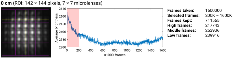
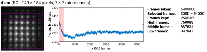
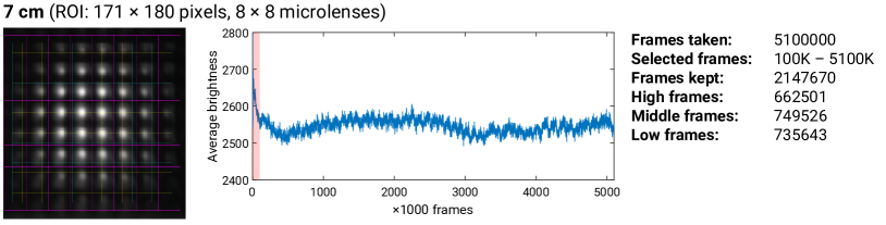
In our experiments, the thresholding process is that pixels whose grayscale values (from to ) are greater than are recorded as . The top lines in the frames are cropped to avoid abnormal dark counts caused by the EMCCD, and the images are then rotated by to undo the effect of the imaging lens. We define the brightness of a frame as the number of pixels whose . A graph of the average brightness per frames is plotted, and a subset from the original image data is selected to ensure the variation range of the average brightness per frames is about (or less than) (Fig. 7 provides the brightness graph and the subset selection of each experiment). In our brightness separation formula, the average brightness of frames of the subset is calculated. Then, one frame is named:
(1) low frame if its brightness satisfies ;
(2) middle frame if ;
(3) high frame if ;
(4) otherwise it is discarded.
Letting be the number of low, middle and high frames respectively, and be (similar expressions for and ), the JPD is calculated by
| (8) |
which can be understood as , where are from the covariance formula of low, middle, high frames respectively. Calculating respectively can avoid the background from the brightness fluctuation. Weighting according to reduces the impact of covariance error from a lower number of frames (As can be seen in Fig. 7, are approximately equal for each experiment, so the impact is not significant). If all frames are of one type (e.g. middle) and not discarded (defining when ), this formula reverts to the original covariance formula times the number of frames.
The JPD of the same pixel cannot be measured in principle [6], and counts of two pixels on the same line have abnormal correlation (The closer they are, the stronger the correlation is) from the mechanism of EMCCD, so we use interpolation to eliminate these effects. If the two pixels and satisfy and , is replaced by (if takes the top or bottom value, it is or respectively).
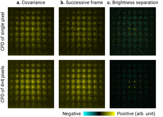
Here we also use the other two formulas to calculate the single-pixel CPDs and their sums over given pixels as shown in Fig. 2, and compare them with our formula. We find that the bright spots are also visible, but the background noises are significant. Using the brightness separation formula, the JPD values in regions with no coincidence are mainly negative, possibly because the sub-Poissonian photon statistics after frame discarding introduces a slightly negative background.
The methods and algorithms used in our experiments are not perfect, and can be improved in the future.
E. Details of the calculation of the aperture CPD and the phase gradient
In this section, we describe the data processing from single-pixel CPDs to aperture CPDs. An illustration of its principle is shown in Fig. 3. First, we evaluate the direct image (the sum of all the thresholded frames) and determine the position of the apertures (See Fig. 7). The apertures used in our calculations are not necessarily the same as the microlenses. In the SPDC biphoton propagation data, the apertures used in data processing are larger to contain the whole spot.
All pixels completely inside each aperture are considered in the calculation. However, if the CPDs of them are directly summed, the result is distorted (Lines where the given points lie are brighter than other lines) due to the abnormal correlation of EMCCD. Fig. 4 shows direct summations of single-pixel CPDs over regions with different sizes, ranging from the original single-pixel CPD ( pixel) to the sum over almost the whole aperture ( pixels). We find that summing over pixels has a better performance.
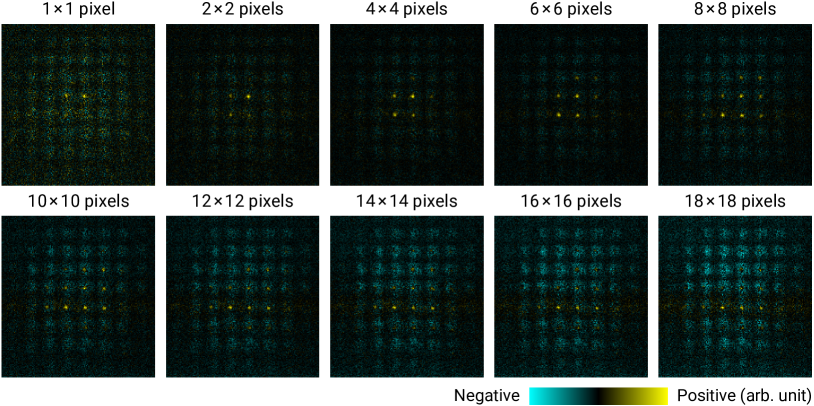

In our data processing, each aperture is divided into -pixel segments (segments near the right and top border of the aperture may be smaller), and the (or fewer) CPDs of each segment are summed first (as shown in the process from Fig. 5b to 5c). The result goes through the noise reduction process. In each aperture, the maximum value is found and all negative values are set to zero. The values inside a region centered by the maximum pixel are subtracted by the average value of pixels adjacent to the region (i.e., inside a region centered by the maximum pixel excluding the region), so that the background is subtracted (negative values can be introduced again). Finally, pixels outside the region are set to zero.
After noise reduction, the CPDs of all the -pixel segments are summed, as shown in Fig. 5e, and negative values of the sum are set to zero. This becomes the final aperture CPD. Fig. 6 also provides the calculated aperture CPDs with various segment sizes. Sizes ranging from to pixels can all yield a satisfactory result with less noise or amplitude distortion.
When calculating the phase gradient distribution from an aperture CPD, a -pixel region with the largest CPD sum is chosen, and the region centered by the region is used to calculate the centroid position of the spot relative to the microlens center (The rest of the aperture is believed to have no light spot, and does not contribute to the calculation).
F. The phase reconstruction algorithm
With the phase gradient distributions , to realize the line integral in Eq. (2) of the main text, we use the computer algorithm based on random point spreading and averaging in our previous work [3], whose steps are as follows:
(1) Select the point with the maximum JPD as the starting point whose phase is . A thread-safe queue is used and the point is enqueued. The phase values of all other points are marked as “not calculated”. Mark the status of all threads as “unfinished” and start multiple threads ( threads in our experiments).
(2) A single thread attempts to dequeue a point. If the queue is empty, go to step (3). Otherwise, the thread marks its status as “unfinished”, checks how many adjacent points (up to points) of the dequeued one are not calculated, and then probabilistically chooses whether to calculate the phase of the adjacent point based on the zonal method formula and enqueue it, or to ignore it. Denoting the coordinates of the dequeued point as ( are integers), the basic expansion formulas are, for example,
| (9) |
where is the spacing of the discretized gradient distributions (i.e., microlens aperture width divided by the interpolation times). If the JPD of the dequeued point is smaller, the probability of calculation is also smaller due to larger errors. After handling all the adjacent points, if any adjacent points are ignored (still not calculated), the dequeued point is enqueued again. This thread repeats this step.
(3) This thread marks the thread status as “finished”, checks the status of all other threads. If there are “unfinished” threads, go back to step (2).
(4) One phase reconstruction process is done. Record the phase distribution.
(5) To reduce errors, repeat the above process several times ( times in our experiments) and take the average phase of each time as the reconstruction result.
G. Details of the experimental data
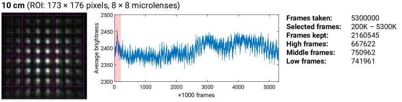
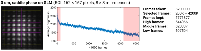
Fig. 7 shows the direct images from the EMCCD, ROI sizes, the average brightness values per frames, frame counts of each experiment. Inside the direct images, yellow grids indicate the microlens centers, cyan grids indicate the microlens borders, and magenta grids indicate the actual aperture division in data processing (If the actual aperture size equals the microlens size, the magenta grid covers the cyan one). Only a part of the frames is selected to ensure the brightness fluctuation is within , and frames discarded manually are painted as light red in the graphs.
H. Theory of degenerate collinear type-I SPDC and double-Gaussian parameters
From the phase matching condition of , assuming the pump beam is monochromatic and the transverse size of the BBO crystal is large enough so that the transverse phase matching is precise, the joint angular spectrum (wave function in the momentum space) of the degenerate down-converted photons is
| (10) |
where the symbols , and stand for pump ( light), signal ( light) and idler ( light) photon respectively, is the angular spectrum of the pump beam, and is the crystal thickness. From the birefringent theory,
| (11) | |||
| (12) |
where is the frequency (invariant in media) of the light considered, is the speed of light in vacuum,
| (13) |
and is the angle between the optical axis of the crystal (in the - plane) and the surface normal line [8]. The Sellmeier equations of and of BBO can be found in Ref. [9]. For degenerate collinear type-I SPDC with the pump beam at , and .
Denoting the wave number in vacuum as (), considering the collinear phase matching, and ignoring the walk-off effect determined by , when , we have and
| (14) |
| (15) |
If the pump beam is Gaussian with its waist at the crystal , its angular spectrum is . However, the term hinders further analytical expressions, and should be approximated by a Gaussian function. We follow the method by Chan et al. that when , [10]. Letting , the wave function takes the double-Gaussian form in Eqs. (3) and (4) of the main text.
In our experiment, the double-Gaussian parameters of photon pairs at the BBO are mm and µm. The three Fourier lenses are equivalent to one lens with the focal length cm. and at its focal plane (the -cm position of the microlens array) are approximately µm and mm respectively, which are used to calculate the theoretical wave function after propagating a distance. The theoretical distance with no amplitude correlation is cm.
I. Theoretical and experimental wave functions and their Fourier transforms
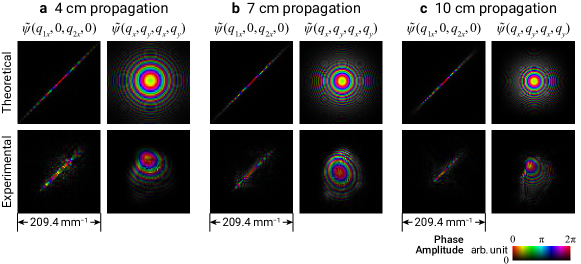
Fig. 8 provides nine conditional wave functions for each theoretical and experimental case except the -cm one (with no propagation). The phase pattern of conditional wave function anti-correlates with the given point.
We perform discrete Fourier transform on the theoretical and experimental wave functions to show the biphoton wave function in momentum space. and are positively correlated, and the global paraboloid phase from the angular spectrum theory becomes steeper as increases. Fig. 9 shows two slices of each momentum wave function, and . Errors of the JPD and phase make their Fourier transforms distorted, but the momentum correlation and the global phase pattern can still be seen.
J. Analysis of classically correlated two-photon states
Ignoring normalization, we consider this type of classically correlated state whose density matrix is
| (16) |
where
| (17) |
is the Gaussian state with the center , the waist radius and distance . This is an ensemble of photon pairs having the same Gaussian spatial profile with opposite centers. We assume the photons are distinguishable (e.g. the two beams are spatially separated) and only consider here, so the photons are anti-correlated in position. The spatial JPD is
| (18) |
which is the same as the entangled state represented by the squared modulus of Eq. (3) of the main text.
After propagating a distance , the third parameters in the states in Eq. (16) are switched to . In the one-dimensional case (), We calculate the probability distribution first:
| (19) |
After plotting (shown in Fig. 10), we find that as increases, the two photons are less anti-correlated, but they will never show positive correlation. When is very large, the photons at the far field has almost no position correlation.
Now we consider the QSHWS of this mixed state. Each pure component has an uncorrelated position JPD contribution on the back focal plane of the microlens array, and the JPDs of different components of the mixed state are directly summed. Each component has a different phase gradient distribution, so if we obtain the CPD of an accurate point at the sensor, one can tell which component it is from. However, if we calculate the CPD of an aperture, the spots in the CPD have sizes much larger than the usual Airy spot. If the average positions of the spots are used to calculate the so-called “phase gradient” (In the one-dimensional case, it is just the partial derivative), assuming the microlens is small, and letting (second-order coherence function), the measured “phase gradient” of photon 2 with a given position of photon 1 is [2,3]
| (20) |
Given , the “gradient” is still a linear function of , so the “phase distribution” also has a quadratic form. Compared to the entangled case
| (21) |
when , take the theoretical values in our experiment and , the joint wave function of the entangled photons and the reconstructed “wave function” of the classically correlated photons are shown in Fig. 11, where the experimentally reconstructed wave function using the -cm data is also given. When the given point changes, the center of the parabolic “phase” pattern of the conditional “wave function” moves backward slower than , while for the entangled case, the center of phase pattern moves almost at the same speed. These features make the classically correlated state different from the entangled state. The single-pixel CPD may provide more information about the properties of the unknown two-photon field, and this can be further explored in the future.
K. Derivation of the convolution formula
Here we provide a derivation of Eq. (5) in the main text:
| (22) |
The convolution sign on the last line only acts on ( is treated as a constant).
References
[1] Jorge Ares, Teresa Mancebo, and Salvador Bará, Position and displacement sensing with Shack–Hartmann wave-front sensors, Appl. Opt. 39, 1511 (2000).
[2] Y. Zheng, M. Yang, Z.-H. Liu, J.-S. Xu, C.-F. Li, and G.-C. Guo, Detecting momentum weak value: Shack–Hartmann versus a weak measurement wavefront sensor, Opt. Lett. 46, 5352 (2021).
[3] Y. Zheng, M. Yang, Y.-W. Liao, J.-S. Xu, C.-F. Li, and G.-C. Guo, Reconstructing the multiphoton spatial wave function with coincidence wave-front sensing, Phys. Rev. A 107, 042608 (2023).
[4] H. Defienne, M. Reichert, and J. W. Fleischer, General Model of Photon-Pair Detection with an Image Sensor, Phys. Rev. Lett. 120, 203604 (2018).
[5] M. Reichert, H. Defienne, and J. W. Fleischer, Optimizing the signal-to-noise ratio of biphoton distribution measurements, Phys. Rev. A 98, 013841 (2018).
[6] H. Defienne, M. Reichert, J. W. Fleischer, and D. Faccio, Quantum image distillation, Sci. Adv. 5, eaax0307 (2019).
[7] H. Defienne, B. Ndagano, A. Lyons, and D. Faccio, Polarization entanglement-enabled quantum holography, Nat. Phys. 17, 591 (2021).
[8] S. Walborn, C. Monken, S. Pádua, and P. Souto Ribeiro, Spatial correlations in parametric down-conversion, Phys. Rep. 495, 87 (2010).
[9] D. Eimerl, L. Davis, S. Velsko, E. K. Graham and A. Zalkin, Optical, mechanical, and thermal properties of barium borate, J. Appl. Phys. 62, 1968 (1987).
[10] K. W. Chan, J. P. Torres, and J. H. Eberly, Transverse entanglement migration in Hilbert space, Phys. Rev. A 75, 050101 (2007).