Measuring the circular polarization
of gravitational waves with
pulsar timing arrays
N. M. Jiménez Cruza 111nmjc1209.at.gmail.com, Ameek Malhotraa 222ameek.malhotra.at.swansea.ac.uk, Gianmassimo Tasinatoa,b 333g.tasinato2208.at.gmail.com, Ivonne Zavalaa 444e.i.zavalacarrasco.at.swansea.ac.uk
a Physics Department, Swansea University, SA28PP, United Kingdom
b Dipartimento di Fisica e Astronomia, Università di Bologna,
INFN, Sezione di Bologna, I.S. FLAG, viale B. Pichat 6/2, 40127 Bologna, Italy
Abstract
The circular polarization of the stochastic gravitational wave background (SGWB) is a key observable for characterising the origin of the signal detected by Pulsar Timing Array (PTA) collaborations. Both the astrophysical and the cosmological SGWB can have a sizeable amount of circular polarization, due to Poisson fluctuations in the source properties for the former, and to parity violating processes in the early universe for the latter. Its measurement is challenging since PTA are blind to the circular polarization monopole, forcing us to turn to anisotropies for detection. We study the sensitivity of current and future PTA datasets to circular polarization anisotropies, focusing on realistic modelling of intrinsic and kinematic anisotropies for astrophysical and cosmological scenarios respectively. Our results indicate that the expected level of circular polarization for the astrophysical SGWB should be within the reach of near future datasets, while for cosmological SGWB circular polarization is a viable target for more advanced SKA-type experiments.
1 Introduction
The recent hints of detection of a stochastic gravitational wave background (SGWB) by several pulsar timing arrays (PTA) collaborations [1, 2, 3, 4, 5] raise questions about its origin, whether astrophysical or cosmological: see respectively [6, 7] and [8] for reviews, and [9] for a recent assessment on the challenges to distinguish among different SGWB sources with PTA experiments. The amount of circular polarization imprinted in the SGWB constitutes a possible discriminator among the two possibilities. Several early universe sources can induce a circularly polarized SGWB, for example associated with phenomena of parity violation in gravitational or vector sectors, see e.g. [10, 11, 12, 13, 14, 15, 16, 17, 18]. Moreover, an astrophysical SGWB is also characterized by a sizeable amount of circular polarization, related with the distribution of inclination angles of black hole binary sources [19, 20]. But a measurement of circular polarization with PTA, although interesting, is challenging since the isotropic part of the background is insensitive to this quantity [21]. The reason being the geometrical configuration of the PTA system, which makes its response to circular polarization vanish. This feature is in common with what happens for planar GW interferometric detectors, such as LISA (see e.g. [22, 23, 24, 25, 26]). Hence, an option for detecting the SGWB circular polarization with PTA is to measure SGWB anisotropies: see e.g. [21, 27, 28, 29, 30], and [31] for a review. For cosmological sources, anisotropies are induced by early universe effects, and an approach to describe SGWB anisotropies and their properties in this context has been recently developed (see e.g. [32, 33, 34, 35, 36, 37, 38, 39, 40, 41, 42]). For astrophysical sources, SGWB anisotropies arise due to clustering of galaxies where the GW sources reside, as well as Poisson-type fluctuations [43, 44, 45, 46, 47, 48, 49, 50, 29, 20, 51, 52]. SGWB anisotropies have not been measured yet with PTA experiments [53, 51], but given their rich physics content their detectability represents an active an interesting line of investigation – see e.g. [54, 45, 44, 55, 56, 57, 27, 58, 59, 60, 61, 62].
The aim of this work is to forecast the sensitivity of PTA experiments to circular polarization, making use for the first time of realistic modelling of SGWB anisotropies. We study the two options of cosmological and astrophysical SGWB.
For the first case of GW sources from the early universe, the largest contribution to SGWB anisotropies is associated to kinematic Doppler effects, due to our motion with respect to the source of SGWB [40, 63]. They are the GW analog to kinematic effects measured in the cosmic microwave background radiation [64, 65, 66, 67, 68]. Kinematic anisotropies in the SGWB are deterministically controlled by the isotropic part of the background, and the amplitude of the kinematic dipole is expected to be of order smaller than the isotropic monopole. The PTA response to kinematic anisotropies can be analytically computed [54, 44, 30], including the effects of circular polarization, and modified gravity signatures [30]. In [69] we forecasted the sensitivity of future PTA experiments to kinematic effects related to the SGWB intensity. In the present work, sections 2, 3 and 4, we study using different approaches how the measurement of kinematic anisotropies can be used to detect the circular polarization of the cosmological background with future PTA data. We find that monitoring a large number of monitored pulsars will be necessary to detect the signal we are interested in.
A more optimistic result is obtained investigating the case of astrophysical SGWB, studied in section 5. For such a GW signal, the degree of intrinsic anisotropy is sizeable, of order up to relative to the monopole, hence much larger than the kinematic one [43, 44, 45, 46, 47, 48, 49, 50, 29, 20]. Interestingly, the astrophysical SGWB is expected to be strongly circularly polarized [19, 20], with an amplitude of circular polarization comparable to the SGWB intensity – this property of course improves the prospects of detection. In fact, our analysis suggests that a monitoring few hundred pulsars (which should be achievable in the SKA era [70, 71, 72]) should be sufficient for detecting circular polarization in the astrophysical SGWB.
We conclude in section 6. We adopt units in which .
2 Our set-up
We start with a theoretical section, based on [30], reviewing the formulas needed for our analysis. We focus in this section on kinematic anisotropies only, with the amplitude of the kinematic dipole of order with respect to the background monopole. We then have in mind cosmological sources for the SGWB, as explained in the introduction. Other works discussing kinematic effects on SGWB include [40, 63, 73, 74, 75, 76, 77]. A discussion of intrinsic anisotropies for astrophysical backgrounds, and the associated measurement of circular polarization, can be found in section 5.
Gravitational waves (GW) are fluctuations around the Minkowski metric
| (2.1) |
They are decomposed in Fourier modes as
| (2.2) |
imposing the condition , which ensures that is real. We adopt a basis for the polarization tensors in eq (2.2); we assume they are real.
Pulsar timing arrays (PTA) measure GW through the time delay they cause on the observed pulsar period. Such time delays are associated with GW deformations of light geodesics from emission to detection. We denote pulsars with latin letters: , , etc. The time delay associated with pulsar is denoted with . We decompose it in Fourier modes as
| (2.3) | |||||
The detector tensor is defined in terms of polarization tensors as . The quantity is the pulsar position, and is the light travelling time from emission to detection.
We express the GW two-point correlators as (we use notation of [23, 78]):
| (2.4) |
The quantity is decomposed into intensity and circular polarization:
| (2.5) |
where the tensor components are , while .
The SGWB intensity is real and positive. The circular polarization is a real quantity. Both quantities can depend on the GW frequency and direction, and behave as scalars under boosts. We introduce the short-hand notation
| (2.6) |
and compute the two-point correlator between two pulsar time-delays, associated with a pulsar pair and . We find (we sum over repeated indexes)
This formula indicates that circular polarization is only detectable at unequal time measurements: (see e.g. [24]). It is convenient to make use of time residuals
| (2.8) |
a quantity easier to handle when Fourier transforming the signal. Their two-point function is
where is the isotropic value of the intensity integrated over all directions, while is its analog for circular polarization. In writing eq (2) we introduce
| (2.11) | |||||
and
| (2.12) | |||||
with denoting dot product, and cross product among vectors. In passing from eq (2) to eq (2) we integrate along directions, and we define the PTA response functions
| (2.13) | |||||
| (2.14) |
The response functions are key quantities to study the response of the PTA system to GW observables.
We can avoid to carry on the oscillating functions in the integrand of eq (2), and define
| (2.15) |
In fact, the quantities , in eq (2) indicate that we are measuring pulsar signals at different times, separated by an interval corresponding to the ‘cadence’ of detection. PTA collaborations measure pulsar periods around once per week: the cadence then establishes the upper bound in frequency of PTA measurements yr Hz. Hence, we typically work in a regime where . Consequently, the oscillating functions in the integrand of eq (2) are expected to give order one factors, and will be neglected in the definition of the two-point function passing from (2) to (2.15). See e.g. [79], chapter 23.
While so far our formulas are general, we now focus on kinematic anisotropies, following the treatment of [69, 30]. Our motion with velocity with respect to the SGWB rest frame, induces kinematic anisotropies in intensity and circular polarization . They are expressed as
| (2.16) |
with
| (2.17) |
where is the GW direction, and the relative velocity among frames. Since in this and the next section we are assuming a cosmological origin for the SGWB, we expect to be of the same order of the value measured by cosmic microwave background: [64, 65, 66, 67, 68]. With being small, we can expand both quantities in (2.16) at first order in , and plug the resulting expressions in the response functions of eqs (2.13), (2.14). In this way, we determine the PTA response to the kinematic dipole in intensity and in circular polarization. Defining , , we obtain
| (2.18) | |||||
| (2.19) |
with
| (2.20) | |||||
| (2.21) | |||||
| (2.22) |
with . As stated in the introduction, the PTA response to circular polarization vanishes for an isotropic background. In fact, the response of eq (2.19) is non-zero only in the presence of anisotropies, since it starts at first order in the expansion.
While corresponds to the well-known Hellings-Downs response to the isotropic part of the background, the two contributions and control the PTA response to the kinematic dipole (respectively to the intensity and circular polarization of the GW).
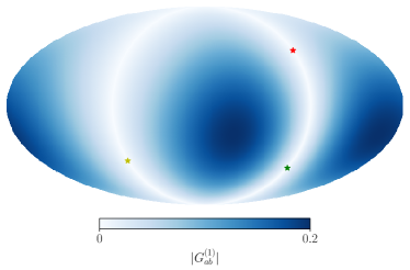
Interestingly, while the PTA response is more sensitive to the intensity kinematic dipole when pulsar vectors lie parallely to the velocity vector (see eq (2.21) – we studied this phenomenon in [69]), the opposite is true for the circular polarization dipole [30], which can be measured more easily with pulsars located orthogonally to (see eq (2.22)). See e.g. Fig 1 for a graphical representation of the quantity . This property implies that an appropriate choice of the pulsars to measure – depending on their position – can make enhance the sensitivity on the signal. We will make use of this feature in what follows.
These results complete the review of the theoretical tools we can apply to the forecast of detectability of circular polarization with PTA experiments, a topic we discuss next.
3 Circular polarization and present-day PTA experiments
After reviewing and developing in section 2 the theoretical basis for our work, we discuss practical strategies for detecting circular polarization with PTA data. As we learned, the detection of circular polarization is tied with the measurement of SGWB anisotropies.
We forecast the prospects to detect the SGWB circular polarization by measuring the kinematic dipole of the SGWB with PTA. In this section we have in mind a cosmological SGWB which can have a potentially large amplitude of circular polarization, as large as the SGWB intensity, see e.g. [10, 11, 12, 13, 14, 15, 16, 18, 80, 81, 82, 83, 84]. Interestingly, also the astrophysical SGWB is expected to be characterized by a large amount of circular polarization: we discuss it in section 5.
We proceed following two approaches. First, in this section, we focus on near future PTA experiments in the SKA era [70, 71, 72], which will monitor a finite number (of order few hundreds) pulsars. Building on the results of section 2, we show how the sensitivity to circular polarization can improve by choosing carefully the position in the sky of the monitored pulsars. It is very hard though to reach a level of sensitivity compatible with a detection. In the next section 4, then, we make some simplifying assumptions to study the problem, and we examine the case of futuristic PTA experiments monitoring very large (of order thousands) pulsars. In such a case, the experiments will have enough sensitivity to detect the effects we are interested about.
Other works discussing prospects of detection of circular polarization with PTA, also following alternative methods, are [21, 27, 28, 29]. As far as we are aware, ours is the first work which makes use of realistic modelling of SGWB anisotropies (both for cosmological and astrophysical sources) towards the detection of .
We assume that the isotropic part of intensity and circular polarization – obtained integrating over all angular directions – follows a power-law profile given by
| (3.1) |
with a reference frequency (we take yr-1, as appropriate for PTA experiments), while and are the tilts defined above eq (2.18). The constant quantities and control the amplitude of intensity and circular polarization. Following the conventions of [1] we introduce the constants and as
| (3.2) |
as alternative parameters to test. The definition (3.2) allows us to compare more directly with the results of [1].
3.1 Limits from current datasets, and definition of the likelihood
We focus here on PTA experiments with a finite number of monitored pulsars. We take the NANOGrav configuration system [85, 86, 87, 88] as reference. The NANOGrav collaboration collects data monitoring 67 pulsars. First, we show that the sensitivity of current version of the NANOGrav pulsar system is not sufficient to detect a signal associated with the SGWB circular polarization . To improve the situation, we then imagine to add a finite number (up to few hundred) of monitored pulsars to the NANOGrav pulsar set. For definiteness, we adopt the same noise curves of the NANOGrav pulsars [86], and we locate the additional objects at appropriate positions in the sky in order to be more sensitive to circular polarization.
To start with, we make use of publicly available tools and assess to what extent current can PTA data set useful constraints on SGWB circular polarization. We analyse the NANOGrav data set [1] (referred to as NG15 hereafter) looking for the presence of circular polarization through the kinematic dipole. We fix the dipole magnitude and direction to be the same as the cosmic microwave background [67]. We apply the likelihood made available by the NANOGrav collaboration through the packages ENTERPRISE [89] and ENTERPRISE-EXTENSIONS [90]. We explore the parameter space using the MCMC sampler [91, 92], through the Cobaya interface [93]. We vary the SGWB intensity amplitude , the spectral tilt in the combination
the relative circular polarization amplitude 555While the parameter runs between -1 and 1, from now on in our Fisher forecasts we only will consider its absolute value and take it to be positive.
| (3.3) |
and we fix the individual pulsar red noise parameters to their median values from the NG15 analyses for computational ease. The key parameter controlling the amplitude of circular polarization versus intensity is .
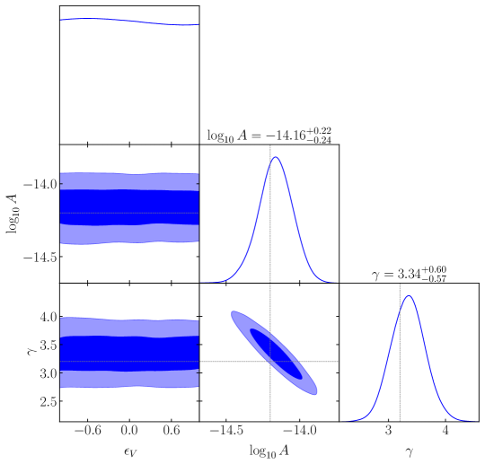
We plot the marginalised distributions for the SGWB parameters in Fig 2 using GetDist [94]. The figure shows that current data are in fact unable to put any constraints on the magnitude of circular polarization. The reason can be understood as follows. As we have learned above PTA systems are blind to the circular polarization monopole, thus we need to measure the SGWB anisotropy to detect it. But, as shown in [69], current data impose only an upper limit on the kinematic dipolar anisotropy. Thus, by fixing , can be freely varied within its prior range without creating significant deviations from the observed inter-pulsar correlations.666Varying the individual pulsar red noise parameters will not change our results, since the circular polarization is essentially unconstrained at the moment.
To improve on the current situation, a possibility is to monitor additional pulsars appropriately located in the sky (following the criteria of section 2), so to collect more information specifically on the SGWB circular polarization. This is the strategy we adopt in this section. To study this option, we introduce a Gaussian likelihood for intensity and circular polarization, and , making use of ideas first developed in [58]:
| (3.4) |
In the previous formula, we follow the same notation of [69], extending it by including the circular polarization contribution . (We refer the reader to [58, 69] for more information on this method.) The sum runs over pulsar pairs, each pair indicated with a capital letter . The dot in eq (3.4) indicates a bandwidth-integrated quantity, centered around the frequency , hence
| (3.5) |
and analogously for . The are the measured cross-correlations of time residuals. The are the PTA response functions to intensity and circular polarization, discussed in section 2. The quantity is the inverse of the covariance matrix. We make the hypothesis to work here in the weak signal limit (more on this in the next section). The covariance matrix can then be approximated as [58, 69]:
| (3.6) |
with the time of observation of the four pulsars , and with the band integrated noise variance for pulsar . Given a vector of observable parameters we wish to probe, the Fisher information criteria (see e.g. [95]) allow us to forecast the ability of future experiments to measure . The best fit correspond to values of which makes vanishing the first derivative of the likelihood: . The experimental errors on the parameter determination, then, is expressed in terms of the second-derivatives of the log-likelihood, i.e. the Fisher matrix:
| (3.7) |
where indicates we evaluate the log-likelihood second derivative at the parameter best fit values.
Armed with this formalism, we investigate in this section how to use a PTA system to probe to circular polarization for cosmological SGWB, making use of the kinematic dipole. We wish to forecast the size of experimental error bars for a set of GW parameters. We assume the benchmark values listed in Table 1 for the parameters entering our formulas, where the quantities are introduced in eqs (3.2). We examine a situation characterized by a large degree of circular polarization , of the same order of the intensity; such a case can be realized in early universe scenarios where phenomena of parity violation occur in the gravitational sector. (For the case of astrophysical SGWB, see section 5.) For the intensity parameter we take as reference the central value measured by the NANOGrav collaboration [1]. The values characterizing the kinematic dipole are the ones obtained by CMB experiments, and we use galactic coordinates to express the velocity. For the rest of this section we consider two cases, corresponding to two different vectors of parameters to be tested.
3.2 Case 1: forecasts on parameters , , and
We forecast the ability of PTA to measure the amplitude of circular polarization (equivalently ), as well as the SGWB intensity (equivalently ) and kinematic dipole amplitude . In the presence of large values of , a measurement of circular polarization gives us also information on the velocity parameter characterizing kinematic anisotropies. The parameter vector to be measured is then . The PTA pulsar set we consider is constituted by the 67 NANOGrav pulsars, to which we add more pulsars located at appropriate positions to increase the sensitivity to the observables of interest (see section 2).
The symmetric Fisher matrix is computed following the definition in eq (3.7). When evaluated at a given frequency it results (we write each matrix component at leading order in a small expansion)
with
| (3.9) |
Starting from these equations, the complete Fisher matrix is obtained by summing over the individual frequency bins, . We notice that off-diagonal terms in (LABEL:fishrea) induce correlations in the measurements of the parameters we are interested in. As a consequence a measurement of the kinematic parameter is facilitated in the presence of large values of and/or , when monitoring pulsars located at appropriate positions.
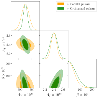
To exemplify these statements, we examine four different scenarios, with the main aim to quantify how the number and location of the pulsars to monitor affects the size of the error bars in the measurement of the quantities we are interested in. For each scenario, we forecast the size of error bars on the parameters using the Fisher formalism (see Table 2) and we plot them using GetDist [94], see Figures 3 and 4. For each scenario, we add one (or multiple) set(s) of 67 pulsars, characterized by the same noise properties of the 67 NANOGrav ones [87], located at appropriate positions in the sky to investigate the effects we are more interested on.
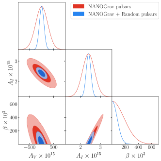
Scenario 1
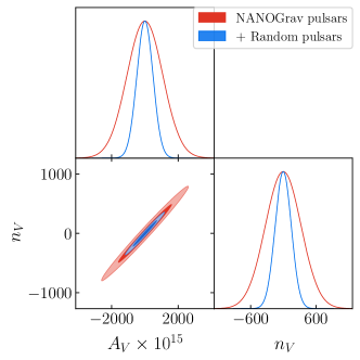
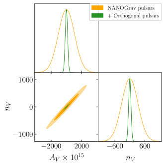
In a first scenario, shown in Fig 3, upper left panel, we consider the same pulsar set monitored by the NANOGrav collaboration [85, 86, 87, 88] (red colour, scenario ), and we add to this set 67 randomly located pulsars (blue color, scenario ). Our aim is to understand how the addition of pulsars at random positions reduces the error bars. In passing from scenario to the errors on and decrease by more than a factor of 2 (see Table 2), although also for scenario they are still large. The measurement of , which can be obtained by the study of the isotropic part of SGWB with no need of detecting anisotropies, is very accurate, with a relative error of order one percent.
Scenario 2
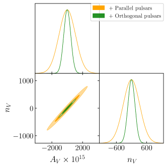
In a second scenario, see Fig 3, upper right panel, we instead add pulsars at positions parallel (yellow color, scenario ) or orthogonal (green color, scenario ) to the direction of frame velocity (we assume for the new pulsars the same noise curves as NANOGrav pulsars). We learned in section 2 that when monitoring pulsars located with these criteria we increase the sensitivity to (respectively) intensity and circular polarization of the SGWB (see [30, 69]). In fact, the yellow ellipses in Fig 3 (upper right panel) demonstrate that measurements of do not result more accurate with respect to the case of NANOGrav pulsars only (compare with the upper left panel in the same figure). At the same time, the green ellipses show that, as expected, the accuracy in measuring increases and the error halves its size. See the error bars in Table 2 for quantitative estimate of the errors.
Scenario 3
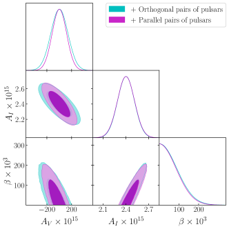
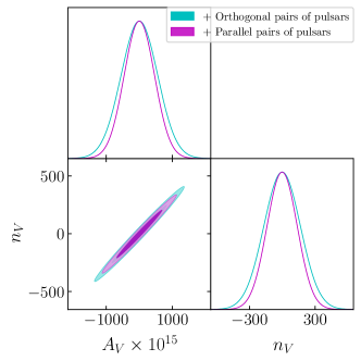
In the third scenario, see Fig 3 lower left panel, we focus on investigating from another viewpoint the sensitivity of the PTA system to circular polarization. We start from noticing that eq (2.22) indicates that the sensitivity to increases when the condition is satisfied. This condition requires that is perpendicular to the pulsar directions (a case already explored in the previous scenario 2), and additionally that is parallel to . To analyse this particular case, we consider the 67 NANOGrav pulsars, and we select what we call pulsar at the position of pulsar B1937+21 [86]. We then generate 67 extra pulsars to monitor, with positional vectors satisfying the condition : we call this scenario . Similarly, we generate 67 extra pulsars with positional vectors satisfying the condition : this is scenario . We expect that while the sensitivity to increases in scenario , it is reduced in the scenario , also with respect to the original 67 NANOGrav set. This behaviour is confirmed by Fig 3, lower left panel.
Scenario 4
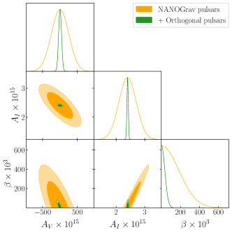
The analysis of the previous three scenarios shows that adding just 67 more pulsars to the NANOGrav data set is not sufficient to reach the accuracy for an informative measurement of circular polarization, even if the pulsars are located to the most convenient positions. In the fourth scenario we explore the possibility of adding four extra sets of 67 pulsars each to the original NANOGrav set (hence, in total, we have 335 pulsars to monitor). The new pulsars are located orthogonally to the velocity , and each set of 67 pulsars uses the same noise curves of the 67 NANOGrav pulsars [87]. The results are represented in Fig 3, lower right panel, while the error bars are in Table 2. We notice that the sensitivity to circular polarization is much improved with respect to the previous scenarios (i.e. we gain a factor 8 in sensitivity with respect to NANOGrav pulsar set). However the error bars are still relatively large. We now proceed to investigate whether the situation changes by consider a different set of parameters to constrain.
3.3 Case 2: Forecasts on the parameters ,
As a second case, we focus on the measurement of parameters , assuming we already have information on the remaining parameters in the benchmark set of Table 1, which enter the likelihood function. Hence we wish to make use of kinematic anisotropies not only to probe the amplitude, but also the slope of the circular polarization spectrum: see the definition in eq (3.1). The corresponding Fisher matrix, evaluated in a Taylor expansion up order , results
| (3.10) | |||||
We consider in this context the same four scenarios examined in section 3.2. We represent our results in Fig 4, and report the corresponding error bar estimate in table 3.
In the first scenario, upper left panel of Fig. 4, we learn that the error bars on and decrease their size (by a factor one half) with increasing the number of pulsars to detect, as expected. In the second scenario, upper right panel of Fig. 4, we learn that the error bars are blind to the addition of pulsars, as expected from our theory formulas of section 2. Instead, the error bar sizes decrease considerably adding pulsars located orthogonally to the velocity among frames (see lower left panel of Fig 4) . The same behaviour is confirmed in the fourth scenario plotted in the lower right panel of Fig 4.
Still, the error bars in the parameters are quite large, even for scenario .To reduce the error bars of our forecasts to a level acceptable for ensuring detection, we discuss in section 4 a method to analytically explore more futuristic set ups able to considerably enhance the sensitivity to circular polarization, by increasing the number of pulsars to be monitored.
4 Futuristic set up: isotropically distributed pulsars
We learned in the previous section that adding pulsars at specific positions certainly improves the detectability prospects of circular polarization , but not enough to ensure detection. In this section, following ideas first developed in [58], we focus on an idealized scenario which simplifies our calculations and allow for analytical estimates of the expected accuracy obtained with future measurements.
We consider a futuristic setup of PTA monitoring a a large number of pulsars, say in the order of thousands, and we take eq (3.4) for our likelihood. For developing our analytical arguments, we make the following hypothesis:
-
•
We assume the pulsars are isotropically distributed across the sky, they have the same properties, and they are monitored for the same amount of time.
- •
These simplifying assumptions allow us to approach the problem analytically, using the Fisher formalism of [58].
We assume that the properties of the SGWB intensity (including the kinematic dipole) are already known, thus we fix to the values used in the previous section, see Table 1.777Our choice of fixing the intensity parameters for the Fisher forecasts – instead of considering them as additional parameters to be measured simultaneously – will be justified in what comes next.
Analogously to what done in the literature for the intensity of the SGWB [58, 69], in our limit of a large number of identical, isotropically distributed pulsars we obtain the following Fisher matrix for the circular polarization parameters, evaluated at fixed frequency
| (4.1) |
where is given in eq (3.1), and in eq (2.12). This Fisher component should then be summed over frequencies, as in the previous section. Following [58] (which focuses on the intensity in the dense pulsar limit), we can convert the sum into an integral, and write
| (4.2) |
We then consider the quantity
| (4.3) | ||||
| (4.4) |
for which for the first time we obtain the following novel analytic expression 888This result can be in principle obtained following the methods of Appendix C of [58]. We found it easier to carry the integrals in the complex plane and use Cauchy theorem, applying in this context the procedure proposed in [96] for computing the Hellings-Downs curve. Please contact the authors for obtaining the Mathematica notebooks leading to eq (4.5).
| (4.5) | |||||
where . Via the approach explained in footnote 8 one can show that the quantity in the weak signal limit, implying that in the limit of a large number of identical pulsars distributed isotropically across the sky, there is no ‘leakage’ of the intensity map into the circular polarization map. This justifies our choice of assuming the intensity is known when performing the Fisher forecasts for circular polarization.
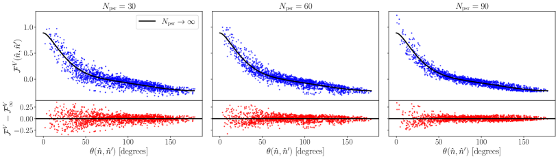
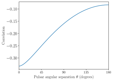
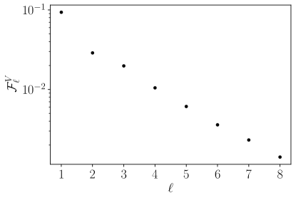
Having calculated (plotted in fig. 5), we can expand it in spherical harmonics (we are justified by the fact that we assume the PTA system to be isotropically distributed in the sky):
| (4.6) |
The spherical harmonic coefficients of in eq (4.6) read . Interestingly, in this idealised full sky limit we find (see [58, 69] for ), which suggests that for sizable polarization, it may be easier to detect the polarization dipole as compared to the dipole relative to the SGWB intensity. The are plotted in fig. 6. Note that – as expected – there is no monopole response, since PTA experiments are blind to the circular polarization monopole.
We do the same for the -mode map, where we consider only the dipole term, the dominant one in a small expansion
| (4.7) |
Substituting the above expressions into our formula for the Fisher matrix evaluated at a given frequency , we find
| (4.8) |
where
| (4.9) |
We now forecast the prospects for future PTA experiments to measure the circular polarization amplitude and the circular polarization tilt introduced in eq (3.1). We find, at leading order in a expansion,
| (4.10) |
Once again, the full Fisher matrix will then be obtained by summing over the individual frequency bins.
We start with the simplest case, and we assume the polarization power law index is the same as the intensity (taken to be : we then fix this quantity. We assume dipole amplitude and direction to be the same as inferred from the CMB (see Table 1) and we first focus on the estimate of only. In this case, the Fisher matrix reduces to
| (4.11) | ||||
where
| (4.12) |
Our PTA setup has the same configuration we used for the intensity forecasts in [69]. We take for the pulsar white noise; we fix as the cadence, and residuals [97]. For the pulsar red-noise, we fix and which are input into Hasasia [98] to obtain the noise curves. Our frequency bins correspond to as the bin width and as the bin centers.
The estimated error in the measurement of is given by,
| (4.13) |
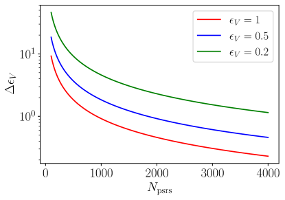
This result is plotted in Fig 7 as a function of for different values of . The figure demonstrates that, under the conditions we are considering, we need at least 1000 pulsars to reach an accuracy sufficient to claim a detection of circular polarization at confidence level greater than 95% for . Definitely, if such futuristic set ups can be achieved, as for example in SKA-type experiments, tests of circular polarization with PTA can be very accurate. On the other hand, for , with such a PTA configuration still remains quite large. We stress that in this section, differently from section 3, we also adopt the same noise curve for each of the pulsars. This choice, along with the fact that we only focus on the polarization amplitude here, reduces considerably the error bars and improves prospects of detection.
As a second case, we now consider both the amplitude and spectral tilt of circular polarization as parameters to be estimated from the data. We express the spectral tilt in terms of the combination
The resulting Fisher matrix is the same as in the first case, up to re-scalings arising from the change of variables to . The fiducial signal parameters are the same as in Case I and we provide forecasts for two different values of . These are plotted in fig. 8.
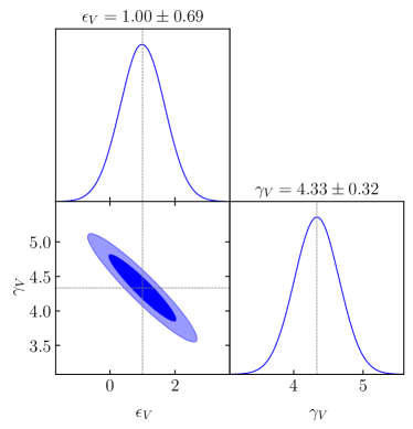
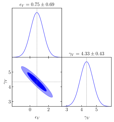
We learn that a maximal level of polarization may be detected with such a PTA whereas for the case, the error bars are large . Notice that when the spectral slope is an additional parameter to be estimated, for the same PTA setup as in [69], the relative error on the amplitude is larger. The main reason being that the circular polarization monopole is not detectable with PTAs, thus if one does not make the assumption that , both the polarization amplitude and spectral tilt have to be estimated together from the anisotropies. This degrades the sensitivity to the amplitude owing to the strong degeneracy between the spectral tilt and the polarization dipole amplitude, as can be seen from (2.19). In fact, the correlation coefficient between and , which is given by , is quite large for the case, indicating that any estimates of the two parameters will be strongly correlated. For this reason, the error bars on are larger compared to those observed in fig. 7.
Note that decreasing the noise level will not directly translate into a reduction in the error bars on and , as one would expect from the form of the Fisher matrix. The reason being that decreases in the noise level will lead to the PTA entering an intermediate or strong-signal regime where the signal to noise ratio only grows as [99]. Indeed, some of the pulsars observed by current PTAs are already in the intermediate signal regime and it is likely that future PTAs will end up being in the strong signal regime. Thus, increasing the number of pulsars observed remains the best bet for more accurate measurement of circular polarization.
This concludes our analysis of cosmological SGWB. In the next section, we will learn that more optimistic prospects of detection are achieved for SGWB of astrophysical origin.
5 Astrophysical SGWB Anisotropies and Circular Polarization
We now consider the case of an astrophysical SGWB. The astrophysical background detectable at PTA frequencies is characterized by significant intrinsic anisotropies, with a relative amplitude of order with respect to the isotropic background (see [51] and references therein). We estimate how a measurement of such intrinsic anisotropies can provide information on the SGWB circular polarization. We will learn that in this case the prospects of detection of this quantity are much more promising as compared to a cosmological background.
A net circular polarization characterizes the SGWB from astrophysical SGWB sources, being generated due to fluctuations in the GW source properties, and the inclination angles of black hole binaries with respect to the line of sight. A quantitative estimate of the net circular polarization due to these effects, relevant for the PTA range was performed in ref. [19, 20] with the result that the circular polarization anisotropies due to such effects have an amplitude quite close to the corresponding intensity anisotropies 999 These estimates of the intensity and polarization anisotropies are based on shot-noise models for the SMBHB and ignore the possible effects of clustering. The circular polarization is generated due to random inclinations of binary orbits with respect to the line-of-sight, so if the inclinations of sources are uncorrelated with the locations, i.e. clustering does not affect inclinations then the relative ratio should still be the same., i.e. , with the same frequency and multipole slope as the intensity.
In this section we calculate the expected SNR with which astrophysical SGWB circular polarization will be detected in future datasets, working in the same idealized framework of section 4. We assume that the angular power spectra of circular polarization scale with and in the same manner as the intensity, i.e.
| (5.1) |
with . We assume that the are independent of , as found in [20, 51]. We calculate the minimum amplitude allowing for a detection of circular polarization, for which we assume a SNR threshold . The SNR (at a given frequency) can be expressed as [58]
| (5.2) |
Expanding the the polarization map and the Fisher matrix in spherical harmonics,
| (5.3) |
the expected value of the becomes
| (5.4) |
The total SNR is obtained by summing over frequencies
| (5.5) |
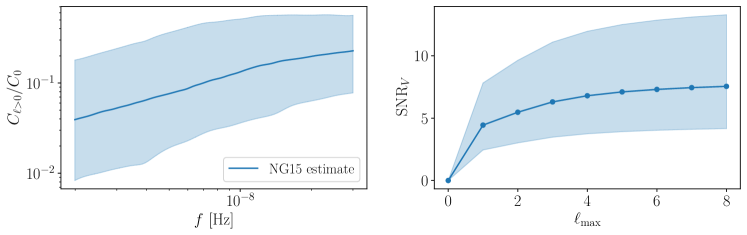
Our results are summarized in Fig. 9, where we plot the SNR of eq. 5.5 as a function of the maximum multipole , for . In this case of maximal circular polarization of the AGWB anisotropies, we find that even 150 pulsars with the selected noise properties may be enough to detect the astrophysical SGWB circular polarization. The much smaller number of pulsars required with respect to cosmological sources (recall section 4) is a consequence of the expected astrophysical SGWB anisotropy being several orders of magnitude larger than the kinematic dipole anisotropy. In the weak signal limit, the corresponding SNR scales with the polarization amplitude and number of pulsars as (see eq. 5.4)
| (5.6) |
Additionally, we can infer that for the PTA setup with many more pulsars to be monitored, say 4000 pulsars as considered in the previous section on cosmological sources, the minimum detectable level of circular polarization is considerably lowered, at the level . The SNR saturates fairly quickly increasing , at around , which can be understood from the fact that the coefficients which represent the PTA sensitivity to circular polarization decrease rapidly with (see fig. 6).
Overall, our results suggest that if the astrophysical SGWB is characterized by a sizeable level of circular polarization, as found in [19, 20], then even near future datasets may be able to set tight constraints on circular polarization. This is especially true since the results of [51] suggest that that the astrophysical SGWB intensity anisotropy may soon be detectable. Even for much smaller levels of SGWB circular polarization, the prospect of detection with an SKA-level experiment is promising. For realistic near future datasets however, we also need to account for the mixing between and anisotropy due to the non-isotropic distribution of a finite number of non-identical pulsars (see eq. (3.2)). We plan to explore the joint estimation of the and anisotropies in future work. Furthermore, note that at present there is some uncertainty in the expected level of astrophysical SGWB intensity anisotropies, so these results might change as our models of the SGWB anisotropy become more and more sophisticated.
6 Conclusions
The polarization content of the SGWB is a key observable that may be used to characterise the background and possibly discriminate between astrophysical and cosmological origin of the signal observed by PTA collaborations. For astrophysical SGWB, net circular polarization may be generated due to fluctuations in the source properties whereas for cosmological sources this would indicate the presence of parity violating physics in the early universe. The detection of circular polarization is made difficult by the fact that PTAs are blind to its monopole, thus we need to observe anisotropies, which are smaller in amplitude and more challenging to detect.
In this paper we have studied the prospects of detecting circular polarization with near and far future PTA experiments, focusing on both astrophysical and cosmological scenarios. On the cosmological side, the largest anisotropy is expected to be generated through kinematic effects for which we analysed the sensitivity of the current datasets (NG15) and future experiments such as the SKA to the circular polarization kinematic dipole. Along the way, we have also highlighted the role played by the positions of the pulsars being observed, as well as the pulsar intrinsic noise properties, in the detection of the dipole and of the SGWB circular polarization. Although the sensitivity of current and near future datasets to the kinematic dipole is limited, a close to maximal polarization may be a realistic target in the SKA era, or in related GW experiments based on astrometry.
For the case of astrophysical SGWB anisotropy, the prospects are much more optimistic. We have shown that the polarization anisotropy is a realistic target for near future experiments if the background is significantly polarised while a polarization level of a few percent may be detectable in the SKA era.
In our discussion, we made optimistic hypothesis on the number and location of pulsars to be monitored, as well as their noise properties. A more sophisticated analysis, considering a fully realistic treatment of the pulsar noise curves, as well as taking into account the role of cosmic variance [50, 100, 101, 102] when monitoring a finite number of pulsars, will be helpful towards clarifying more accurately the prospects of detecting circular polarization with PTA experiments.
Acknowledgments
We are partially funded by the STFC grants ST/T000813/1 and ST/X000648/1. We also acknowledge the support of the Supercomputing Wales project, which is part-funded by the European Regional Development Fund (ERDF) via Welsh Government. For the purpose of open access, the authors have applied a Creative Commons Attribution licence to any Author Accepted Manuscript version arising.
References
- [1] NANOGrav Collaboration, G. Agazie et al., “The NANOGrav 15 yr Data Set: Evidence for a Gravitational-wave Background,” Astrophys. J. Lett. 951 no. 1, (2023) L8, arXiv:2306.16213 [astro-ph.HE].
- [2] D. J. Reardon et al., “Search for an Isotropic Gravitational-wave Background with the Parkes Pulsar Timing Array,” Astrophys. J. Lett. 951 no. 1, (2023) L6, arXiv:2306.16215 [astro-ph.HE].
- [3] H. Xu et al., “Searching for the Nano-Hertz Stochastic Gravitational Wave Background with the Chinese Pulsar Timing Array Data Release I,” Res. Astron. Astrophys. 23 no. 7, (2023) 075024, arXiv:2306.16216 [astro-ph.HE].
- [4] EPTA, InPTA: Collaboration, J. Antoniadis et al., “The second data release from the European Pulsar Timing Array - III. Search for gravitational wave signals,” Astron. Astrophys. 678 (6, 2023) A50, arXiv:2306.16214 [astro-ph.HE].
- [5] International Pulsar Timing Array Collaboration, G. Agazie et al., “Comparing recent PTA results on the nanohertz stochastic gravitational wave background,” arXiv:2309.00693 [astro-ph.HE].
- [6] A. Sesana, A. Vecchio, and C. N. Colacino, “The stochastic gravitational-wave background from massive black hole binary systems: implications for observations with Pulsar Timing Arrays,” Mon. Not. Roy. Astron. Soc. 390 (2008) 192, arXiv:0804.4476 [astro-ph].
- [7] S. Burke-Spolaor et al., “The Astrophysics of Nanohertz Gravitational Waves,” Astron. Astrophys. Rev. 27 no. 1, (2019) 5, arXiv:1811.08826 [astro-ph.HE].
- [8] C. Caprini and D. G. Figueroa, “Cosmological Backgrounds of Gravitational Waves,” Class. Quant. Grav. 35 no. 16, (Aug., 2018) 163001, arXiv:1801.04268 [astro-ph.CO]. https://iopscience.iop.org/article/10.1088/1361-6382/aac608.
- [9] S. Babak, M. Falxa, G. Franciolini, and M. Pieroni, “Forecasting the sensitivity of Pulsar Timing Arrays to gravitational wave backgrounds,” arXiv:2404.02864 [astro-ph.CO].
- [10] R. Jackiw and S. Y. Pi, “Chern-Simons modification of general relativity,” Phys. Rev. D 68 (2003) 104012, arXiv:gr-qc/0308071.
- [11] A. Lue, L.-M. Wang, and M. Kamionkowski, “Cosmological signature of new parity violating interactions,” Phys. Rev. Lett. 83 (1999) 1506–1509, arXiv:astro-ph/9812088.
- [12] M. Satoh, S. Kanno, and J. Soda, “Circular Polarization of Primordial Gravitational Waves in String-inspired Inflationary Cosmology,” Phys. Rev. D 77 (2008) 023526, arXiv:0706.3585 [astro-ph].
- [13] C. R. Contaldi, J. Magueijo, and L. Smolin, “Anomalous CMB polarization and gravitational chirality,” Phys. Rev. Lett. 101 (2008) 141101, arXiv:0806.3082 [astro-ph].
- [14] S. Alexander and N. Yunes, “Chern-Simons Modified General Relativity,” Phys. Rept. 480 (2009) 1–55, arXiv:0907.2562 [hep-th].
- [15] M. M. Anber and L. Sorbo, “Non-Gaussianities and chiral gravitational waves in natural steep inflation,” Phys. Rev. D 85 (2012) 123537, arXiv:1203.5849 [astro-ph.CO].
- [16] N. Bartolo et al., “Science with the space-based interferometer LISA. IV: Probing inflation with gravitational waves,” JCAP 12 (2016) 026, arXiv:1610.06481 [astro-ph.CO].
- [17] E. Dimastrogiovanni, M. Fasiello, and T. Fujita, “Primordial Gravitational Waves from Axion-Gauge Fields Dynamics,” JCAP 01 (2017) 019, arXiv:1608.04216 [astro-ph.CO].
- [18] A. Nishizawa and T. Kobayashi, “Parity-violating gravity and GW170817,” Phys. Rev. D 98 no. 12, (2018) 124018, arXiv:1809.00815 [gr-qc].
- [19] L. Valbusa Dall’Armi, A. Nishizawa, A. Ricciardone, and S. Matarrese, “Circular Polarization of the Astrophysical Gravitational Wave Background,” Phys. Rev. Lett. 131 no. 4, (2023) 041401, arXiv:2301.08205 [astro-ph.CO].
- [20] G. Sato-Polito and M. Kamionkowski, “Exploring the spectrum of stochastic gravitational-wave anisotropies with pulsar timing arrays,” arXiv:2305.05690 [astro-ph.CO].
- [21] R. Kato and J. Soda, “Probing circular polarization in stochastic gravitational wave background with pulsar timing arrays,” Phys. Rev. D 93 no. 6, (2016) 062003, arXiv:1512.09139 [gr-qc].
- [22] N. Seto, “Prospects for direct detection of circular polarization of gravitational-wave background,” Phys. Rev. Lett. 97 (2006) 151101, arXiv:astro-ph/0609504.
- [23] T. L. Smith and R. Caldwell, “Sensitivity to a Frequency-Dependent Circular Polarization in an Isotropic Stochastic Gravitational Wave Background,” Phys. Rev. D 95 no. 4, (2017) 044036, arXiv:1609.05901 [gr-qc].
- [24] V. Domcke, J. Garcia-Bellido, M. Peloso, M. Pieroni, A. Ricciardone, L. Sorbo, and G. Tasinato, “Measuring the net circular polarization of the stochastic gravitational wave background with interferometers,” JCAP 05 (2020) 028, arXiv:1910.08052 [astro-ph.CO].
- [25] LISA Cosmology Working Group Collaboration, P. Auclair et al., “Cosmology with the Laser Interferometer Space Antenna,” Living Rev. Rel. 26 no. 1, (2023) 5, arXiv:2204.05434 [astro-ph.CO].
- [26] M. Colpi et al., “LISA Definition Study Report,” arXiv:2402.07571 [astro-ph.CO].
- [27] S. C. Hotinli, M. Kamionkowski, and A. H. Jaffe, “The search for anisotropy in the gravitational-wave background with pulsar-timing arrays,” Open J. Astrophys. 2 no. 1, (2019) 8, arXiv:1904.05348 [astro-ph.CO].
- [28] E. Belgacem and M. Kamionkowski, “Chirality of the gravitational-wave background and pulsar-timing arrays,” Phys. Rev. D 102 no. 2, (2020) 023004, arXiv:2004.05480 [astro-ph.CO].
- [29] G. Sato-Polito and M. Kamionkowski, “Pulsar-timing measurement of the circular polarization of the stochastic gravitational-wave background,” Phys. Rev. D 106 no. 2, (2022) 023004, arXiv:2111.05867 [astro-ph.CO].
- [30] G. Tasinato, “Kinematic anisotropies and pulsar timing arrays,” Phys. Rev. D 108 no. 10, (2023) 103521, arXiv:2309.00403 [gr-qc].
- [31] J. D. Romano and N. J. Cornish, “Detection methods for stochastic gravitational-wave backgrounds: a unified treatment,” Living Rev. Rel. 20 no. 1, (Dec., 2017) 2, arXiv:1608.06889 [gr-qc]. http://link.springer.com/10.1007/s41114-017-0004-1.
- [32] V. Alba and J. Maldacena, “Primordial gravity wave background anisotropies,” JHEP 03 (2016) 115, arXiv:1512.01531 [hep-th].
- [33] C. R. Contaldi, “Anisotropies of Gravitational Wave Backgrounds: A Line Of Sight Approach,” Phys. Lett. B 771 (2017) 9–12, arXiv:1609.08168 [astro-ph.CO].
- [34] M. Geller, A. Hook, R. Sundrum, and Y. Tsai, “Primordial Anisotropies in the Gravitational Wave Background from Cosmological Phase Transitions,” Phys. Rev. Lett. 121 no. 20, (2018) 201303, arXiv:1803.10780 [hep-ph].
- [35] N. Bartolo, D. Bertacca, S. Matarrese, M. Peloso, A. Ricciardone, A. Riotto, and G. Tasinato, “Anisotropies and non-Gaussianity of the Cosmological Gravitational Wave Background,” Phys. Rev. D 100 no. 12, (2019) 121501, arXiv:1908.00527 [astro-ph.CO].
- [36] N. Bartolo, D. Bertacca, V. De Luca, G. Franciolini, S. Matarrese, M. Peloso, A. Ricciardone, A. Riotto, and G. Tasinato, “Gravitational wave anisotropies from primordial black holes,” JCAP 02 (2020) 028, arXiv:1909.12619 [astro-ph.CO].
- [37] N. Bartolo, D. Bertacca, S. Matarrese, M. Peloso, A. Ricciardone, A. Riotto, and G. Tasinato, “Characterizing the cosmological gravitational wave background: Anisotropies and non-Gaussianity,” Phys. Rev. D 102 no. 2, (2020) 023527, arXiv:1912.09433 [astro-ph.CO].
- [38] P. Adshead, N. Afshordi, E. Dimastrogiovanni, M. Fasiello, E. A. Lim, and G. Tasinato, “Multimessenger Cosmology: correlating CMB and SGWB measurements,” Phys. Rev. D 103 no. 2, (2021) 023532, arXiv:2004.06619 [astro-ph.CO].
- [39] L. Valbusa Dall’Armi, A. Ricciardone, N. Bartolo, D. Bertacca, and S. Matarrese, “Imprint of relativistic particles on the anisotropies of the stochastic gravitational-wave background,” Phys. Rev. D 103 no. 2, (2021) 023522, arXiv:2007.01215 [astro-ph.CO].
- [40] LISA Cosmology Working Group Collaboration, N. Bartolo et al., “Probing anisotropies of the Stochastic Gravitational Wave Background with LISA,” JCAP 11 (2022) 009, arXiv:2201.08782 [astro-ph.CO].
- [41] A. Malhotra, E. Dimastrogiovanni, G. Domènech, M. Fasiello, and G. Tasinato, “New universal property of cosmological gravitational wave anisotropies,” Phys. Rev. D 107 no. 10, (2023) 103502, arXiv:2212.10316 [gr-qc].
- [42] F. Schulze, L. Valbusa Dall’Armi, J. Lesgourgues, A. Ricciardone, N. Bartolo, D. Bertacca, C. Fidler, and S. Matarrese, “GWCLASS: Cosmological Gravitational Wave Background in the Cosmic Linear Anisotropy Solving System,” arXiv:2305.01602 [gr-qc].
- [43] N. J. Cornish and A. Sesana, “Pulsar Timing Array Analysis for Black Hole Backgrounds,” Class. Quant. Grav. 30 (2013) 224005, arXiv:1305.0326 [gr-qc].
- [44] C. M. Mingarelli, T. Sidery, I. Mandel, and A. Vecchio, “Characterizing gravitational wave stochastic background anisotropy with pulsar timing arrays,” Phys. Rev. D 88 no. 6, (2013) 062005, arXiv:1306.5394 [astro-ph.HE].
- [45] S. R. Taylor and J. R. Gair, “Searching For Anisotropic Gravitational-wave Backgrounds Using Pulsar Timing Arrays,” Phys. Rev. D 88 (2013) 084001, arXiv:1306.5395 [gr-qc].
- [46] C. M. F. Mingarelli, T. J. W. Lazio, A. Sesana, J. E. Greene, J. A. Ellis, C.-P. Ma, S. Croft, S. Burke-Spolaor, and S. R. Taylor, “The local nanohertz gravitational-wave landscape from supermassive black hole binaries,” Nature Astronomy 1 no. 12, (Nov., 2017) 886–892, arXiv:1708.03491 [astro-ph.GA].
- [47] N. J. Cornish and L. Sampson, “Towards Robust Gravitational Wave Detection with Pulsar Timing Arrays,” Phys. Rev. D 93 no. 10, (2016) 104047, arXiv:1512.06829 [gr-qc].
- [48] S. R. Taylor, R. van Haasteren, and A. Sesana, “From Bright Binaries To Bumpy Backgrounds: Mapping Realistic Gravitational Wave Skies With Pulsar-Timing Arrays,” Phys. Rev. D 102 no. 8, (2020) 084039, arXiv:2006.04810 [astro-ph.IM].
- [49] B. Bécsy, N. J. Cornish, and L. Z. Kelley, “Exploring Realistic Nanohertz Gravitational-wave Backgrounds,” Astrophys. J. 941 no. 2, (2022) 119, arXiv:2207.01607 [astro-ph.HE].
- [50] B. Allen, “Variance of the Hellings-Downs correlation,” Phys. Rev. D 107 no. 4, (2023) 043018, arXiv:2205.05637 [gr-qc].
- [51] NANOGrav Collaboration, G. Agazie et al., “The NANOGrav 15-year Data Set: Search for Anisotropy in the Gravitational-Wave Background,” (6, 2023) , arXiv:2306.16221 [astro-ph.HE].
- [52] M. R. Sah, S. Mukherjee, V. Saeedzadeh, A. Babul, M. Tremmel, and T. R. Quinn, “Imprints of Supermassive Black Hole Evolution on the Spectral and Spatial Anisotropy of Nano-Hertz Stochastic Gravitational-Wave Background,” arXiv:2404.14508 [astro-ph.CO].
- [53] S. R. Taylor et al., “Limits on anisotropy in the nanohertz stochastic gravitational-wave background,” Phys. Rev. Lett. 115 no. 4, (2015) 041101, arXiv:1506.08817 [astro-ph.HE].
- [54] M. Anholm, S. Ballmer, J. D. E. Creighton, L. R. Price, and X. Siemens, “Optimal strategies for gravitational wave stochastic background searches in pulsar timing data,” Phys. Rev. D 79 (2009) 084030, arXiv:0809.0701 [gr-qc].
- [55] J. Gair, J. D. Romano, S. Taylor, and C. M. F. Mingarelli, “Mapping gravitational-wave backgrounds using methods from CMB analysis: Application to pulsar timing arrays,” Phys. Rev. D 90 no. 8, (2014) 082001, arXiv:1406.4664 [gr-qc].
- [56] N. J. Cornish and R. van Haasteren, “Mapping the nano-Hertz gravitational wave sky,” arXiv:1406.4511 [gr-qc].
- [57] C. M. F. Mingarelli, T. J. W. Lazio, A. Sesana, J. E. Greene, J. A. Ellis, C.-P. Ma, S. Croft, S. Burke-Spolaor, and S. R. Taylor, “The Local Nanohertz Gravitational-Wave Landscape From Supermassive Black Hole Binaries,” Nature Astron. 1 no. 12, (2017) 886–892, arXiv:1708.03491 [astro-ph.GA].
- [58] Y. Ali-Haïmoud, T. L. Smith, and C. M. F. Mingarelli, “Fisher formalism for anisotropic gravitational-wave background searches with pulsar timing arrays,” Phys. Rev. D 102 no. 12, (2020) 122005, arXiv:2006.14570 [gr-qc].
- [59] Y. Ali-Haïmoud, T. L. Smith, and C. M. F. Mingarelli, “Insights into searches for anisotropies in the nanohertz gravitational-wave background,” Phys. Rev. D 103 no. 4, (2021) 042009, arXiv:2010.13958 [gr-qc].
- [60] N. Pol, S. R. Taylor, and J. D. Romano, “Forecasting Pulsar Timing Array Sensitivity to Anisotropy in the Stochastic Gravitational Wave Background,” Astrophys. J. 940 no. 2, (2022) 173, arXiv:2206.09936 [astro-ph.HE].
- [61] R. C. Bernardo, G.-C. Liu, and K.-W. Ng, “Correlations for an anisotropic polarized stochastic gravitational wave background in pulsar timing arrays,” arXiv:2312.03383 [gr-qc].
- [62] J. Nay, K. K. Boddy, T. L. Smith, and C. M. F. Mingarelli, “Harmonic Analysis for Pulsar Timing Arrays,” arXiv:2306.06168 [gr-qc].
- [63] G. Cusin and G. Tasinato, “Doppler boosting the stochastic gravitational wave background,” JCAP 08 no. 08, (2022) 036, arXiv:2201.10464 [astro-ph.CO].
- [64] G. F. Smoot, M. V. Gorenstein, and R. A. Muller, “Detection of Anisotropy in the Cosmic Black Body Radiation,” Phys. Rev. Lett. 39 (1977) 898.
- [65] A. Kogut et al., “Dipole anisotropy in the COBE DMR first year sky maps,” Astrophys. J. 419 (1993) 1, arXiv:astro-ph/9312056.
- [66] WMAP Collaboration, C. L. Bennett et al., “First year Wilkinson Microwave Anisotropy Probe (WMAP) observations: Preliminary maps and basic results,” Astrophys. J. Suppl. 148 (2003) 1–27, arXiv:astro-ph/0302207.
- [67] WMAP Collaboration, G. Hinshaw et al., “Five-Year Wilkinson Microwave Anisotropy Probe (WMAP) Observations: Data Processing, Sky Maps, and Basic Results,” Astrophys. J. Suppl. 180 (2009) 225–245, arXiv:0803.0732 [astro-ph].
- [68] Planck Collaboration, N. Aghanim et al., “Planck 2013 results. XXVII. Doppler boosting of the CMB: Eppur si muove,” Astron. Astrophys. 571 (2014) A27, arXiv:1303.5087 [astro-ph.CO].
- [69] N. M. J. Cruz, A. Malhotra, G. Tasinato, and I. Zavala, “Measuring kinematic anisotropies with pulsar timing arrays,” arXiv:2402.17312 [gr-qc].
- [70] G. Janssen et al., “Gravitational wave astronomy with the SKA,” PoS AASKA14 (2015) 037, arXiv:1501.00127 [astro-ph.IM].
- [71] E. F. Keane et al., “A Cosmic Census of Radio Pulsars with the SKA,” PoS AASKA14 (2015) 040, arXiv:1501.00056 [astro-ph.IM].
- [72] A. Weltman et al., “Fundamental physics with the Square Kilometre Array,” Publ. Astron. Soc. Austral. 37 (2020) e002, arXiv:1810.02680 [astro-ph.CO].
- [73] D. Bertacca, A. Ricciardone, N. Bellomo, A. C. Jenkins, S. Matarrese, A. Raccanelli, T. Regimbau, and M. Sakellariadou, “Projection effects on the observed angular spectrum of the astrophysical stochastic gravitational wave background,” Phys. Rev. D 101 no. 10, (2020) 103513, arXiv:1909.11627 [astro-ph.CO].
- [74] L. Valbusa Dall’Armi, A. Ricciardone, and D. Bertacca, “The dipole of the astrophysical gravitational-wave background,” JCAP 11 (2022) 040, arXiv:2206.02747 [astro-ph.CO].
- [75] A. K.-W. Chung, A. C. Jenkins, J. D. Romano, and M. Sakellariadou, “Targeted search for the kinematic dipole of the gravitational-wave background,” Phys. Rev. D 106 no. 8, (2022) 082005, arXiv:2208.01330 [gr-qc].
- [76] D. Chowdhury, G. Tasinato, and I. Zavala, “Response of the Einstein Telescope to Doppler anisotropies,” Phys. Rev. D 107 no. 8, (2023) 083516, arXiv:2209.05770 [gr-qc].
- [77] G. Cusin, C. Pitrou, C. Bonvin, A. Barrau, and K. Martineau, “Boosting gravitational waves: a review of kinematic effects on amplitude, polarization, frequency and energy density,” arXiv:2405.01297 [gr-qc].
- [78] T. L. Smith and R. Caldwell, “LISA for Cosmologists: Calculating the Signal-to-Noise Ratio for Stochastic and Deterministic Sources,” Phys. Rev. D 100 no. 10, (Nov., 2019) 104055, arXiv:1908.00546 [astro-ph.CO]. http://arxiv.org/abs/1908.00546. arXiv: 1908.00546.
- [79] M. Maggiore, Gravitational Waves: Volume 2. Oxford University Press, 03, 2018. https://doi.org/10.1093/oso/9780198570899.001.0001.
- [80] D. G. Figueroa, M. Pieroni, A. Ricciardone, and P. Simakachorn, “Cosmological Background Interpretation of Pulsar Timing Array Data,” arXiv:2307.02399 [astro-ph.CO].
- [81] M. Geller, S. Ghosh, S. Lu, and Y. Tsai, “Challenges in interpreting the NANOGrav 15-year dataset as early Universe gravitational waves produced by an ALP induced instability,” Phys. Rev. D 109 no. 6, (2024) 063537, arXiv:2307.03724 [hep-ph].
- [82] J. Ellis, M. Fairbairn, G. Franciolini, G. Hütsi, A. Iovino, M. Lewicki, M. Raidal, J. Urrutia, V. Vaskonen, and H. Veermäe, “What is the source of the PTA GW signal?,” arXiv:2308.08546 [astro-ph.CO].
- [83] C. Unal, A. Papageorgiou, and I. Obata, “Axion-Gauge Dynamics During Inflation as the Origin of Pulsar Timing Array Signals and Primordial Black Holes,” arXiv:2307.02322 [astro-ph.CO].
- [84] E. Dimastrogiovanni, M. Fasiello, M. Michelotti, and L. Pinol, “Primordial Gravitational Waves in non-Minimally Coupled Chromo-Natural Inflation,” arXiv:2303.10718 [astro-ph.CO].
- [85] NANOGrav Collaboration, G. Agazie et al., “The NANOGrav 15 yr Data Set: Detector Characterization and Noise Budget,” Astrophys. J. Lett. 951 no. 1, (2023) L10, arXiv:2306.16218 [astro-ph.HE].
- [86] NANOGrav Collaboration, G. Agazie et al., “The NANOGrav 15 yr Data Set: Observations and Timing of 68 Millisecond Pulsars,” Astrophys. J. Lett. 951 no. 1, (2023) L9, arXiv:2306.16217 [astro-ph.HE].
- [87] NANOGrav Collaboration, “Noise Spectra and Stochastic Background Sensitivity Curve for the NG15-year Dataset,” July, 2023. https://doi.org/10.5281/zenodo.8092346.
- [88] NANOGrav Collaboration, “The nanograv 15-year data set,” Oct., 2023. https://doi.org/10.5281/zenodo.8423265.
- [89] J. A. Ellis, M. Vallisneri, S. R. Taylor, and P. T. Baker, “Enterprise: Enhanced numerical toolbox enabling a robust pulsar inference suite,” Sept., 2020. https://doi.org/10.5281/zenodo.4059815.
- [90] S. R. Taylor, P. T. Baker, J. S. Hazboun, J. Simon, and S. J. Vigeland, “Enterprise˙extensions,” 2021. https://github.com/nanograv/enterprise_extensions. v2.4.3.
- [91] A. Lewis and S. Bridle, “Cosmological parameters from CMB and other data: A Monte Carlo approach,” Phys. Rev. D66 (2002) 103511, arXiv:astro-ph/0205436 [astro-ph]. https://arxiv.org/abs/astro-ph/0205436.
- [92] A. Lewis, “Efficient sampling of fast and slow cosmological parameters,” Phys. Rev. D87 no. 10, (2013) 103529, arXiv:1304.4473 [astro-ph.CO]. https://arxiv.org/abs/1304.4473.
- [93] J. Torrado and A. Lewis, “Cobaya: Code for Bayesian Analysis of hierarchical physical models,” JCAP 05 (2021) 057, arXiv:2005.05290 [astro-ph.IM].
- [94] A. Lewis, “GetDist: a Python package for analysing Monte Carlo samples,” arXiv:1910.13970 [astro-ph.IM].
- [95] M. Tegmark, A. Taylor, and A. Heavens, “Karhunen-Loeve eigenvalue problems in cosmology: How should we tackle large data sets?,” Astrophys. J. 480 (1997) 22, arXiv:astro-ph/9603021.
- [96] F. A. Jenet and J. D. Romano, “Understanding the gravitational-wave Hellings and Downs curve for pulsar timing arrays in terms of sound and electromagnetic waves,” Am. J. Phys. 83 (2015) 635, arXiv:1412.1142 [gr-qc].
- [97] J. S. Hazboun, J. D. Romano, and T. L. Smith, “Realistic sensitivity curves for pulsar timing arrays,” Phys. Rev. D 100 no. 10, (2019) 104028, arXiv:1907.04341 [gr-qc].
- [98] J. S. Hazboun, J. D. Romano, and T. L. Smith, “Hasasia: A python package for pulsar timing array sensitivity curves,” Journal of Open Source Software 4 no. 42, (10, 2019) 1775. https://doi.org/10.21105/joss.01775.
- [99] X. Siemens, J. Ellis, F. Jenet, and J. D. Romano, “The stochastic background: scaling laws and time to detection for pulsar timing arrays,” Class. Quant. Grav. 30 (2013) 224015, arXiv:1305.3196 [astro-ph.IM].
- [100] B. Allen, “Pulsar Timing Array Harmonic Analysis and Source Angular Correlations,” arXiv:2404.05677 [gr-qc].
- [101] N. Grimm, M. Pijnenburg, G. Cusin, and C. Bonvin, “The impact of large-scale galaxy clustering on the variance of the Hellings-Downs correlation,” arXiv:2404.05670 [astro-ph.CO].
- [102] D. Agarwal and J. D. Romano, “Cosmic variance of the Hellings and Downs correlation for ensembles of universes having non-zero angular power spectra,” arXiv:2404.08574 [gr-qc].