Scalar Dark Energy Models and Scalar-Tensor Gravity: Theoretical Explanations for the Accelerated Expansion of Present Universe

Abstract

The reason for the present accelerated expansion of the Universe stands as one of the most profound questions in the realm of science, with deep connections to both cosmology and fundamental physics. From a cosmological point of view, physical models aimed at elucidating the observed expansion can be categorized into two major classes: dark energy and modified gravity. We review various major approaches that employ a single scalar field to account for the accelerating phase of our present Universe. Dynamical system analysis is employed in several important models to seek for cosmological solutions that exhibit an accelerating phase as an attractor. For scalar field models of dark energy, we consistently focus on addressing challenges related to the fine-tuning and coincidence problems in cosmology, as well as exploring potential solutions to them. For scalar-tensor theories and their generalizations, we emphasize the importance of constraints on theoretical parameters to ensure overall consistency with experimental tests. Models or theories that could potentially explain the Hubble tension are also emphasized throughout this review.

Keywords: dark energy, modified gravity, quintessence, dynamical system, cosmology

1 Introduction

In 1998, two independent research groups [1, 2] studying distant Type Ia Supernovae (SN Ia) presented compelling evidence that the expansion of the Universe is not just expanding but actually accelerating. Subsequent observations, which included more in-depth studies of supernovae [3, 4] and independent data from the cosmic microwave background (CMB) radiation [5, 6, 7, 8, 9, 10, 11], the baryon acoustic oscillation (BAO) peak length scale [12, 13, 14, 15, 16, 17, 18], clusters of galaxies [19, 20], and the large-scale structure (LSS) of the Universe [21, 22, 23, 24], confirmed this remarkable acceleration.

According to Einstein’s general theory of relativity without a cosmological constant, if the Universe was primarily filled with ordinary matter and/or radiation, which are the known constituents of the Universe, gravitational interactions would act to slow down the expansion. However, since the Universe is instead found to be accelerating, we are confronted with two intriguing possibilities, dark energy and modified gravity, both of which would have profound implications for our understanding of the Universe and the laws of physics.

The first possibility is that approximately 70% of the energy density of the Universe exists in a new form characterized by negative pressure, referred to as dark energy. When attributing it to the matter sector, dark energy would modify the stress-energy tensor of matters in Einstein’s field equations, leading to the observed acceleration. This novel dark energy component has become central to cosmology, and understanding its nature remains one of the most significant challenges in modern cosmology and fundamental physics.

The second possibility is that general relativity, as formulated by Einstein, breaks down when applied to cosmological scales. In this scenario, a more comprehensive theory, modifying the Einstein-Hilbert action, would be needed to accurately describe the behavior of the Universe, which would lead to changes in the gravitational sector of the field equations.

Extra scalar fields besides the known Higgs field in the Standard Model of particle physics may play a critical role in fundamental physics and provide valuable insights into various aspects of the Universe [25]. Scalar fields naturally arise in unified theories, e.g. the string theory, and contribute to the overall cosmic energy density, offering a plausible explanation for the observed acceleration of the Universe [26, 27]. In the realm of gravitational theories, scalar fields are pivotal in various models of modified gravity, such as in scalar-tensor theories [28, 29, 30, 31]. The scalar field, in addition to the metric, describes gravitational interactions, resulting in predictions that can deviate from those of Einstein’s theory of relativity. These deviations may manifest as changes in the behavior of the gravitational force at different scales and under extreme conditions, like those found near black holes, inside neutron stars, or during the early Universe [32, 33, 34, 35, 36].

The mystery of cosmic acceleration is connected to several pivotal questions in cosmology and fundamental physics [37]. The cosmic acceleration may hold the key to uncovering a successor to Einstein’s theory of gravity. The relatively small energy density of the quantum vacuum could yield insights into concepts such as supersymmetry and superstring. The mechanism governing the ongoing cosmic acceleration might relate to the primordial inflation in cosmology, while the quest to unravel the cause of cosmic acceleration could potentially introduce novel long-range forces or shed light on the enigmatic smallness of neutrino masses in particle physics.

This review basically focuses on models and theories involving a single scalar field. The aim of this review is to theoretically clarify how these models drive the present Universe to undergo an accelerated expansion, with a wide utilization of dynamical system analysis. We typically do not delve into whether these models conform to various observations from SN Ia, CMB and LSS since it usually requires perturbation calculations and further analysis. For such discussions, the readers are directed to specific articles or reviews on observational constraints, such as Refs. [38, 39]. In Section 2, we provide an overview of the historical context of the cosmological constant, tracing its birth from Einstein to its ultimate confirmation with supernova discoveries. The cosmological constant problem is also overviewed in this section. Sections 3 and 4 introduce scalar field models of dark energy and modified gravity theories incorporating a single scalar field, respectively, which offer explanations for the current expansion of the Universe. We list a series of scalar dark energy models in Section 3 to show that it is challenging for them to solve fine-tuning and coincidence problems simultaneously without getting into other troubles. Interacting dark energy models, which have received much attention recently, are also introduced in this section. In Section 4, we additionally provide constraints from terrestrial and Solar System tests of a general class of scalar-tensor gravity. Screening mechanisms are briefly included as well to illustrate how to maintain consistency with experimental results when there is a stronger coupling between the scalar field and matter. A brief summary is provided in the final section.

Throughout the review, we adopt natural units $c=\hbar=1$, and have a metric signature $(-,+,+,+)$. We denote the Planck mass as $m_{\mathrm{Pl}}=G^{-1/2}\simeq 1.22\times 10^{19}\;\mathrm{GeV}$ and the reduced Planck mass as $M_{\mathrm{Pl}}=(8\pi G)^{-1/2}\simeq 2.44\times 10^{18}\;\mathrm{GeV}$, where $G$ is the Newton’s gravitational constant. When the unit $\kappa\equiv 8\pi G=1$ is employed, we will explain it in advance.

2 Cosmological Constant

The field equation in general relativity with the cosmological constant $\Lambda$ is

$$G_{\mu\nu}+\Lambda g_{\mu\nu}=\kappa T_{\mu\nu}^{\mathrm{m}},$$ (2.1)

where $G_{\mu\nu}$, $g_{\mu\nu}$ and $T_{\mu\nu}^{\mathrm{m}}$ are the Einstein tensor, metric tensor, and energy-momentum tensor for matter in the standard model of particle physics, respectively. The theory that adds a cosmological constant term can be considered as the simplest dark energy model. Introducing a cosmological constant to Einstein’s field equations is a reasonable improvement in the framework of general relativity. Since we all know that the metric itself and the Einstein tensor are the only two tensors constructed from the metric and its derivatives up to the second order, that possess vanishing covariant divergences and lead to the local conservation of the energy-momentum tensor.

If one moves the cosmological constant to the right-hand side, Equation (2.1) becomes

$$G_{\mu\nu}=\kappa(T_{\mu\nu}^{\mathrm{m}}+T^{\Lambda}_{\mu\nu}),$$ (2.2)

where

$$T_{\mu\nu}^{\Lambda}=-\frac{\Lambda}{\kappa}g_{\mu\nu}$$ (2.3)

represents the energy-momentum of a new component (dark energy) outside the standard model of particle physics. Compared with the energy-momentum tensor of a perfect fluid

$$T^{\mathrm{pf}}_{\mu\nu}=(\rho_{\mathrm{pf}}+{p_{\mathrm{pf}}})u_{\mu}u_{\nu}+p_{\mathrm{pf}}g_{\mu\nu},$$ (2.4)

one has

$$\rho_{\Lambda}=-{p_{\Lambda}}=\frac{\Lambda}{\kappa},$$ (2.5)

which indicates that this new component has a constant energy density and a negative pressure. As a result, any form of matter with constant energy density will behave as a cosmological constant (and vice versa), because they enter the field equation with the same mathematical structure.

2.1 A Brief History of Cosmological Constant

When the field equation of general relativity was proposed, most physicists, including Einstein himself, believed that the Universe was in a static state. However, the original field equation was not able to describe a non-evolving Universe. To address this, Einstein introduced a new constant of nature and referred to it as the cosmological constant [40]. Incorporating this constant, Einstein obtained his static Universe, which he at first failed to notice that it is unstable [41]. Einstein also believed that the existence of the cosmological constant does not result in any difference on small scales, such as within the Solar system, as long as it is sufficiently small.

In 1929, Hubble made the groundbreaking discovery that distant galaxies are indeed moving away from us, and he presented strong observational evidence for the expansion of the Universe [42]. It indicated that the Universe is dynamic rather than static. Hence, concerning the original motivation, the cosmological constant is no longer needed.

At the end of the last century, the cosmological constant was reintroduced several times to explain problems related to the relatively young Universe age [43], as well as the peaking number counts of quasars at $z\sim 2$ [44], despite it is well-known that the peak has an explanation of astrophysical origin rather than cosmological nowadays. A non-zero cosmological constant was also invoked in order to reconcile the flat Universe predicted by inflation and some other estimations from observations [45, 46].

The final confirmation of a non-zero value of the cosmological constant is from the accurate measurement of the luminosity distance of SN Ia as a function of redshift [1, 2]. To fit the results in the framework of general relativity, the simplest way is to assume that there exists a new cosmic component, besides radiation and matter (including both ordinary matter and dark matter). The new component has a negative pressure, and dominates the Universe’s present energy budget.

2.2 The Cosmological Constant Problem

Although the confrontation of Equation (2.1) with the Solar system and galactic observations have already given an upper bound of the cosmological constant, a tighter constraint comes from larger scale observations [47, 48] that $\Lambda$ is of the same order of the present value of the Hubble parameter $H_{0}$. The corresponding energy density is calculated directly from Equation (2.5),

$$\rho_{\Lambda}\approx\frac{H^{2}_{0}}{8\pi G}\sim 10^{-47}\,\mathrm{GeV}^{4}.$$ (2.6)

Theoretically, the constant energy density associated with quantum vacuum energy is regarded as the source of the cosmological constant. Similar to the ground state of a quantum harmonic oscillator, which possesses a non-zero zero-point energy proportional to the oscillation frequency of its classical counterpart, vacuum-to-vacuum fluctuations arise from the collective contributions of an infinite number of oscillators capable of vibrating at all possible frequencies. A cutoff frequency is required to prevent the divergence of vacuum energy density. The cutoff wavenumber $k_{\mathrm{c}}=m_{\mathrm{Pl}}$ is considered generally, for the belief of the validity of the quantum field theory and general relativity below the Planck scale. Then vacuum energy density has an extremely large value

$$\rho_{\mathrm{vac}}\approx\frac{k^{4}_{\mathrm{c}}}{16\pi^{2}}\sim 10^{74}\,\mathrm{GeV}^{4},$$ (2.7)

which is more than 120 orders of magnitude larger than the observational bound of $\rho_{\Lambda}$. This huge discrepancy is known as the cosmological constant problem, or the vacuum catastrophe.

Hints that the cosmological constant might be non-zero (see Section 2.1) led Zel’dovich to consider the cosmological constant in terms of vacuum energy in 1967 [49], and since then, numerous solutions have been proposed to address this mismatch of energy density [47, 50, 51, 52]. Apart from anthropic principles [47, 53], the solutions can be broadly categorized into three groups. The first one is to establish a unified framework for quantum gravity, specifically in exploring the interplay between quantum vacuum and gravity [54, 55, 56]. The second category is to “eliminate” the vacuum energy. In the context of supersymmetry—an extension of the standard model—the vacuum energy is exactly zero due to the equal number of fermionic and bosonic degrees of freedom [57]. In addition, an alternative approach, called Schwinger’s source theory [58, 59, 60], changes the interpretation of the quantum field theory formalism, and the vacuum energy is no longer needed. The last is to modify the gravity [37, 61], aiming to acquire an effective cosmological constant, which is actrually not an exact resolution of the vacuum catastrophe. However, the modified gravity seems to become more crucial because of the discovery of a tiny but non-zero cosmological constant. If a modified theory of gravity accurately describes the evolution of the Universe and well explains the observations, it is plausible that at least one of the following two statements holds. (I) The vacuum energy of the Universe is either zero or extremely small. It is possible that the quantum zero-point energy of each field is offset by its higher order corrections, or there exists a cancellation mechanism—maybe a hidden symmetry—of vacuum energy among different fields. In such a scenario, one would need to further scrutinize the explanations of experimental evidence for vacuum energy like the Casimir effect, and the vacuum concept associated with quantum chromodynamics and the spontaneous symmetry breaking in the electroweak force. (II) The vacuum energy, being a purely quantum concept, does not function as a source within classical gravity theory that exerts influence on the geometry of spacetime and other degrees of freedom in modified gravity theories, e.g. scalar fields. In this scenario, the connection between quantum field theory and gravity theory poses significant challenges, while the establishment of a unified framework for describing all fundamental forces remains a central pursuit in modern theoretical physics.

3 Dark Energy

In the framework of general relativity, the radiation and barotropic matter, as the only contents of the Universe, cannot induce an accelerated expansion. The concept of dark energy, termed by Turner [62, 63] as a potential constituent of the Universe, propels the ongoing studies of the accelerated expansion. In the standard Lambda Cold Dark Matter ($\Lambda$CDM) model [38], the dark energy is characterized by the presence of a cosmological constant term, which is not dynamical but exerts influence on the evolution of the Universe. Despite being the standard model in cosmology, it is confronted with various theoretical and observational challenges.

• Fine-tuning problem: The current energy density of the estimated cosmological constant in Equation (2.6) is relatively small based on observations, while the theoretical value of the vacuum energy density in Equation (2.7) is significantly larger. In other words, the observed value of energy density conflicts with the possible energy scales and requires fine-tuning if the cosmological constant originates from the vacuum energy density.

• Coincidence problem: The $\Lambda$CDM model suggests a comparable energy density ratio between the matter and the dark energy [11], implying that the expansion of the Universe transitioned from a decelerated to an accelerated phase at a redshift of approximately $z\sim 0.67$ [27]. The problem of why an accelerated expansion should occur now (actually not long ago) in the very long history of the Universe is called the coincidence problem.

• Hubble tension and more: Recent observations have revealed that within the framework of $\Lambda$CDM model, there exists certain tensions between observations from early Universe and late Universe [64], among which the $H_{0}$ and $S_{8}$ tensions are the most well-known ones. The latest observations with the James Webb Space Telescope further confirm the existence of Hubble tension at $8\sigma$ confidence [65].

3.1 Quintessence

A dynamical scalar field as dark energy—the quintessence model—is one of the most popular models for the dark energy. The audiences may be familiar with the similar inflation model that describes the very early stage of the Universe [66, 67]. However, except for the huge discrepancy in the energy scale, the scalar field is the only component in inflation models, while it is just the fifth element of the Universe in the quintessence model. As the first and the simplest model in this review, we will look at the quintessence in more detail. The evolution of the Universe in this model is displayed in Section 3.1.1, and the introduction of the classification and dynamical system analysis of the quintessence model are in Section 3.1.2 and Section 3.1.3, respectively.

The action for the quintessence model is given by [68]

$$S[g^{\mu\nu},\phi,\Psi_{\mathrm{m}}]=S_{\mathrm{EH}}[g^{\mu\nu}]+S_{\mathrm{q}}[g^{\mu\nu},\phi]+S_{\mathrm{m}}[g^{\mu\nu},\Psi_{\mathrm{m}}],$$ (3.1)

where $S_{\mathrm{EH}}=\int\rmd^{4}x\sqrt{-g}R/2\kappa$ is the Einstein-Hilbert action, $S_{\mathrm{m}}=\int\rmd^{4}x\sqrt{-g}\mathcal{L}_{\mathrm{m}}(\Psi_{\mathrm{m}})$ is the action of all possible matter fields, collectively denoted as $\Psi_{\mathrm{m}}$, and

$$S_{\mathrm{q}}=\int\rmd^{4}x\sqrt{-g}\mathcal{L}_{\mathrm{q}}=\int\rmd^{4}x\sqrt{-g}\left[-\frac{1}{2}g^{\mu\nu}\partial_{\mu}\phi\partial_{\nu}\phi-V(\phi)\right],$$ (3.2)

is the action for the quintessence. $V(\phi)$ is the potential of the scalar field and is always assumed to be positive. By variating the action (3.1), equations of motion for the tensor field $g_{\mu\nu}$ and the scalar field $\phi$ are

$$G_{\mu\nu}=\kappa\big{(}T_{\mu\nu}^{\mathrm{m}}+T_{\mu\nu}^{\mathrm{q}}\big{)},$$ (3.3)

$$\square\phi=\frac{dV}{d\phi},$$ (3.4)

where $\square=g^{\mu\nu}\nabla_{\mu}\nabla_{\nu}$, and $T_{\mu\nu}^{\mathrm{m}}$ is the energy-momentum tensor of ordinary matter including dust and radiation,

$$T_{\mu\nu}^{\mathrm{m}}\equiv-\frac{2}{\sqrt{-g}}\frac{\delta(\sqrt{-g}\mathcal{L}_{\mathrm{m}})}{\delta g^{\mu\nu}},$$ (3.5)

and the energy-momentum tensor of quintessence is

$$T_{\mu\nu}^{\mathrm{q}}=\partial_{\mu}\phi\partial_{\nu}\phi-g_{\mu\nu}\left[\frac{1}{2}g^{\alpha\beta}\partial_{\alpha}\phi\partial_{\beta}\phi+V(\phi)\right].$$ (3.6)

Since the scalar field is minimally coupled to the metric, the action (3.1) can be rewritten as

$$S[g^{\mu\nu},\phi,\Psi_{\mathrm{m}}]=S_{\mathrm{EH}}[g^{\mu\nu}]+S^{\prime}_{\mathrm{m}}[g^{\mu\nu},\Psi_{\mathrm{m}},\phi],$$ (3.7)

where $S_{\mathrm{m}}^{\prime}=S_{\mathrm{m}}+S_{\mathrm{q}}$. In such a case, the scalar field in action (3.7) represents the fifth element of the Universe, other than baryons, photons, neutrinos and dark matter that are usually considered in modern cosmology. This dynamical scalar field as a component of the Universe has first been studied by Ratra & Peebles [69] and Wetterich [70] in 1988, and was first called quintessence in a 1998 paper by Caldwell et al. [68].

3.1.1 Evolution of the Universe in the Quintessence Model.

Based upon the assumptions of homogeneity and isotropy of the Universe, which is approximately true on large scales, the Friedmann-Lemaître-Robertson-Walker (FLRW) metric,

$$\rmd s^{2}=-\rmd t^{2}+a^{2}(t)\left(\frac{\rmd r^{2}}{1-Kr^{2}}+r^{2}\rmd\Omega^{2}_{2}\right),$$ (3.8)

is used to describe the geometry of the Universe. Here, $a(t)$ is the scale factor with the cosmic time $t$, and $\rmd\Omega_{2}^{2}=\rmd\theta^{2}+\sin^{2}\theta\rmd\phi^{2}$ is the line element of a 2-sphere. The constant $K$ describes the geometry of the spatial part of the spacetime, with closed, flat, and open Universes corresponding to $K=+1,0,-1$, respectively. In this review, we always assume a flat Universe, which is consistent with current observations [11].

The Friedmann equations are a set of equations that govern the expansion of space in homogeneous and isotropic models of the Universe. Using the FLRW metric, one has

$$3M_{\mathrm{Pl}}^{2}H^{2}=\rho_{\mathrm{m}}+\rho_{\mathrm{q}},$$ (3.9)

$$-2M_{\mathrm{Pl}}^{2}\dot{H}=\rho_{\mathrm{m}}+\rho_{\mathrm{q}}+p_{\mathrm{m}}+p_{\mathrm{q}},$$ (3.10)

where $H=\dot{a}/a$ is the Hubble parameter. The subscripts “$\mathrm{q}$” and “$\mathrm{m}$” represent quintessence and ordinary matter, respectively. Ordinary matter comprises relativistic radiation and non-relativistic dust, denoted by subscripts “$\mathrm{r}$” and “$\mathrm{d}$” respectively in the following. Assuming that the scalar field only depends on the cosmic time, the energy density and pressure of the quintessence field are

$$\rho_{\mathrm{q}}=\frac{1}{2}\dot{\phi}^{2}+V(\phi),$$ (3.11)

$$p_{\mathrm{q}}=\frac{1}{2}\dot{\phi}^{2}-V(\phi),$$ (3.12)

where the overdot denotes the derivative with respect to the cosmic time $t$. Furthermore, local conservation of the energy-momentum tensor gives

$$\dot{\rho}_{\mathrm{m}}+3H(1+w_{\mathrm{m}})\rho_{\mathrm{m}}=0,$$ (3.13)

$$\dot{\rho}_{\mathrm{q}}+3H(1+w_{\mathrm{q}})\rho_{\mathrm{q}}=0,$$ (3.14)

where $w_{\mathrm{m}}=p_{\mathrm{m}}/\rho_{\mathrm{m}}$ and

$$w_{\mathrm{q}}=\frac{p_{\mathrm{q}}}{\rho_{\mathrm{q}}}=\frac{\dot{\phi}^{2}-2V(\phi)}{\dot{\phi}^{2}+2V(\phi)},$$ (3.15)

are parameters in equations of state (EOS). In the slow-roll limit, $\dot{\phi}^{2}\ll V(\phi)$, the parameter $w_{\mathrm{q}}$ goes to $-1$ and the quintessence acts just like the cosmological constant.

For a constant $w_{\mathrm{m}}$, Equation (3.13) gives

$$\rho_{\mathrm{m}}=\bar{\rho}_{\mathrm{m}}a^{-3(1+w_{\mathrm{m}})},$$ (3.16)

while the solution to Equation (3.14) is

$$\rho_{\mathrm{q}}=\bar{\rho}_{\mathrm{q}}\exp\left[-3\int(1+w_{\mathrm{q}})\frac{\rmd a}{a}\right].$$ (3.17)

Here, $\bar{\rho}_{\mathrm{m}}$ and $\bar{\rho}_{\mathrm{q}}$ are integration constants. Figure 1 depicts the evolution of dust and quintessence energy density parameters, as well as the effective EOS parameter of the quintessence model with an exponential potential, over time. The definitions of the quantities in the plot are provided in Section 3.1.3. As observed from Figure 1, to satisfy $\Omega_{\mathrm{d}}\simeq 0.3$ and $\Omega_{\mathrm{q}}\simeq 0.7$ at present and to experience a period of matter dominance, the initial conditions must be chosen carefully.

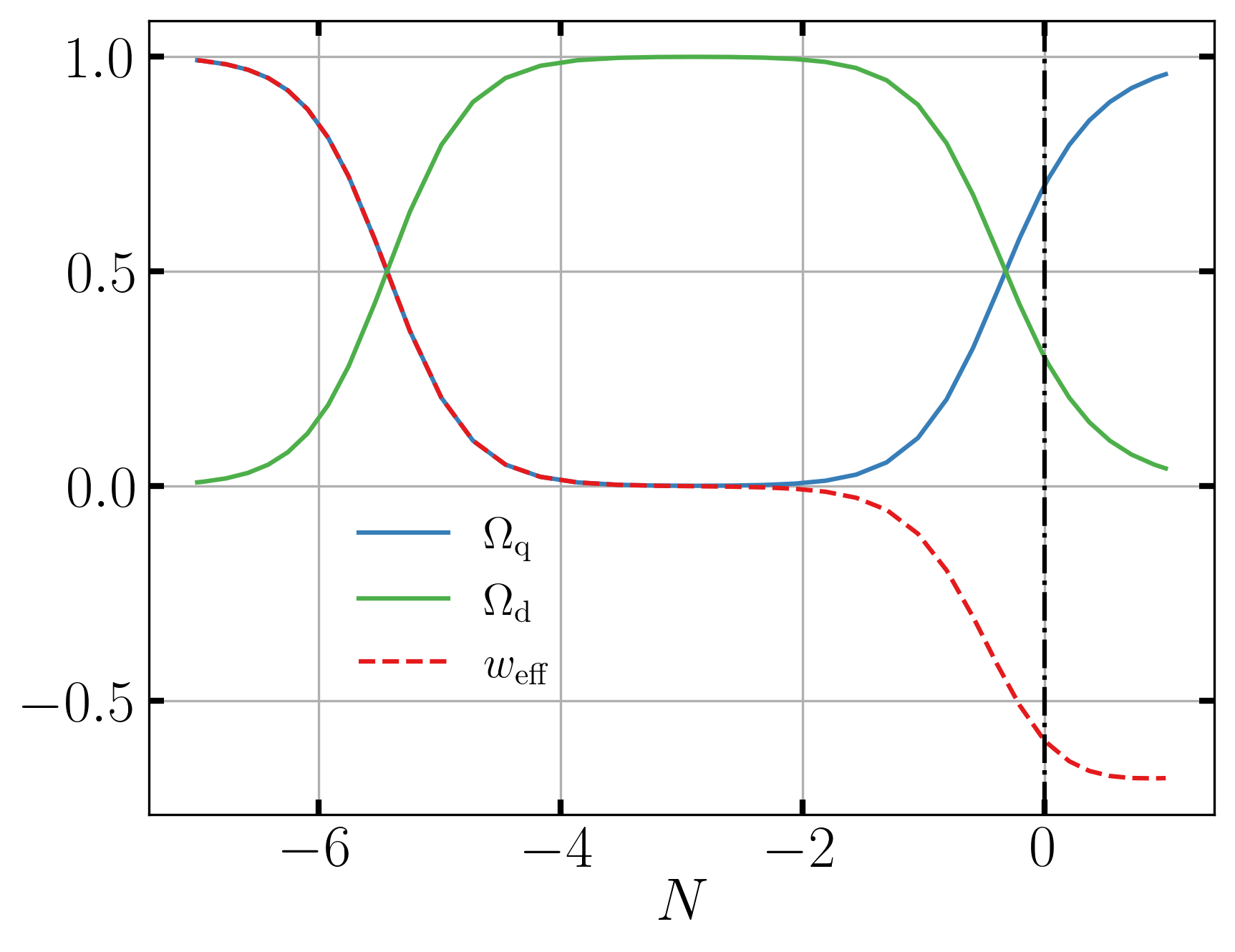
Figure 1: Evolution of the effective EOS parameter $w_{\mathrm{eff}}$, the dust $\Omega_{\mathrm{d}}$ and quintessence $\Omega_{\mathrm{q}}$ relative energy densities with an exponential potential. The vertical dashed line denotes the present cosmological time. One has $\Omega_{\mathrm{d}}\simeq 0.3$ and $\Omega_{\mathrm{q}}\simeq 0.7$ today.

We are currently in a period characterized by the dominance of dark energy. In the quintessence domination, Equations (3.9) and (3.10) become

$$6M_{\mathrm{Pl}}^{2}H^{2}=\dot{\phi}^{2}+2V(\phi),$$ (3.18)

$$-2M_{\mathrm{Pl}}^{2}\dot{H}=\dot{\phi}^{2}.$$ (3.19)

The acceleration equation comes out of a combination of the Friedmann equations, as

$$-3M_{\mathrm{Pl}}^{2}\frac{\ddot{a}}{a}=\frac{1}{2}(\rho_{\mathrm{q}}+3p_{\mathrm{q}})=\dot{\phi}^{2}-V(\phi),$$ (3.20)

which shows that the Universe expands in an increasing rate when $w_{\mathrm{q}}<-1/3$, or $\dot{\phi}^{2}<V(\phi)$. To see how the scalar field evolves, we assume a power-law expansion, $a(t)\propto t^{s}$, where the accelerated expansion occurs for $s>1$. According to Equation (3.19), one obtains

$$\phi=\int\rmd t\sqrt{-2M_{\mathrm{Pl}}^{2}\dot{H}}\propto\ln t.$$ (3.21)

The potential can also be expressed in terms of $H$ and $\dot{H}$ as

$$V=3M_{\mathrm{Pl}}^{2}H^{2}\left(1+\frac{\dot{H}}{3H^{2}}\right)\propto t^{-2}.$$ (3.22)

Combining Equations (3.21) and (3.22), the potential giving the power-law expansion is ought to be an exponential form

$$V(\phi)=\bar{V}\exp\left(-\frac{\lambda\phi}{M_{\mathrm{Pl}}}\right),$$ (3.23)

where $\bar{V}$ is a constant, and $\lambda=\sqrt{2/s}$.

3.1.2 Thawing and Freezing Models.

In the flat FLRW background, Equation (3.4) gives the evolution equation of the quintessence,

$$\ddot{\phi}+3H\dot{\phi}+\frac{\rmd V}{\rmd\phi}=0.$$ (3.24)

Although the presence of ordinary matter is not explicitly accounted for in Equation (3.24), its influence on the Hubble parameter will impact the evolution of the quintessence field. In Equation (3.24), the first term represents the acceleration of the scalar field, while the second term corresponds to a frictional effect, known as Hubble friction or Hubble drag, resulting from the expansion of the Universe, and the third denotes a driving force arising from the steepness of the potential.

The potential function of the scalar field is the only adjustable component in the quintessence model, whose specific shape exerts a significant influence on the cosmic evolution. In order to reproduce the cosmic acceleration today we require that the potential is flat enough to satisfy the condition

$$\left|\frac{M^{2}_{\mathrm{Pl}}}{V}\frac{\rmd^{2}V}{\rmd\phi^{2}}\right|\lesssim 1.$$ (3.25)

Hence, the quintessence mass squared $m^{2}_{\phi}\equiv\rmd^{2}V/\rmd\phi^{2}$ needs to satisfy

$$|m^{2}_{\phi}|\lesssim\frac{V_{0}}{M^{2}_{\mathrm{Pl}}}\sim H_{0}^{2},$$ (3.26)

where $V_{0}$ and $H_{0}$ are the present values of the potential and Hubble parameter, respectively. As a result, the mass of the scalar field has to be extremely small, say $m_{\phi}\lesssim 10^{-33}\;\mathrm{eV}$, to be compatible with the present cosmic acceleration. Apart from this requirement, we also hope that the potential appears in some particle physics models [27].

Caldwell and Linder [71] divided quintessence models into two categories according to whether the scalar field accelerates ($\ddot{\phi}>0$) or decelerates ($\ddot{\phi}<0$). A coasting in the scalar field dynamics, $\ddot{\phi}=0$, is nongeneric, as the field would need to be finely tuned to be perfectly balanced, neither accelerate due to the slope of the potential nor decelerate due to the Hubble drag.

In the accelerating region, the field that has been frozen by the Hubble friction into a cosmological-constant-like state until recently and then begins to evolve gives the thawing model. The current accelerated expansion is driven by the dominance of quintessence and the scalar field in its early stages of “thawing”, implying that $w_{q}$, while increasing, remains smaller than $-1/3$. A representative potential of this class is the one arising from the pseudo Nambu-Goldstone boson [72],

$$V(\phi)=\mu^{4}\left[1+\cos\left(\frac{\phi}{f}\right)\right],$$ (3.27)

where $\mu$ and $f$ are constants characterizing the energy scale and the mass scale of spontaneous symmetry breaking, respectively. If the field mass squared $|m^{2}_{\phi}|\simeq\mu^{4}/f^{2}$ around the potential maximum is smaller than $H^{2}$, the field is stuck there with $w_{\mathrm{q}}\simeq-1$. Once $H^{2}$ drops below $|m^{2}_{\phi}|$, the scalar field starts to move and $w_{\mathrm{q}}$ starts to increase. Likelihood analysis using CMB shift parameters measured by WMAP7 [8] combined with SN Ia and BAO data placed a bound, $w_{\mathrm{q}}|_{z=0}<-0.695$, at the 95 % confidence level, when the quintessence prior is assumed to be $w_{\mathrm{q}}>-1$ [73].

In the decelerating region, the field that initially rolls due to the steepness of the potential but later approaches the cosmological constant state gives the freezing model. A representative potential of this class is the Ratra-Peebles potential [69, 74],

$$V(\phi)=M^{4+n}\phi^{-n},$$ (3.28)

where $M$ and $n$ are positive constants. The potential does not possess a minimum and hence the field rolls down the potential towards infinity. The movement of the field gradually slows down when $\phi$ is large enough and the system enters the phase of cosmic acceleration. Under the quintessence prior $w_{\mathrm{q}}^{\rmi}>-1$ for tracking solutions (see Section 3.1.3), likelihood analysis using the iterative solution in Ref. [75] resulted in bounds, $w_{q}^{\rmi}<-0.923$ and $0.675<\Omega_{\mathrm{q}}<0.703$, at the 95 % confidence level, from the observational data of Planck 2015, SN Ia, and CMB [76]. For the Ratra-Peebles potential, this bound translates to $n<0.17$, which means that the tracker solutions arising from the inverse power-law potential with positive integer powers are observationally excluded.

3.1.3 Dynamical System Approach.

The Universe comprises multiple components, and each of these exerts its own influence on the dynamic evolution of the Universe. The dynamical system approach is a powerful method that helps illustrate the global dynamics and full evolution of the Universe [77, 78]. Through the careful choice of the dynamical variables, a given cosmological model can be written as an autonomous system of some differential equations, which further provides a quick answer to whether it can reproduce the observed expansion of the Universe.

An autonomous system is a system of ordinary differential equations which does not explicitly depend on the independent variable,

$$\frac{\rmd}{\rmd t}\mathbf{x}(t)=f(\mathbf{x}(t)),$$

where $\mathbf{x}$ takes values in $n$-dimensional Euclidean space. Many laws in physics, where $t$ is often interpreted as time, are expressed as autonomous systems because it is always assumed that the laws of nature which hold now are identical to those for any point in the past or future. The time $t$ is usually replaced by the scale factor $a$ or its logarithm in cosmology because the Universe expands monotonously in most of cases so that the scale can be used as a measure of time.

In order to describe the quintessence model, the following dimensionless variables

$$x_{\mathrm{K}}\equiv\frac{\dot{\phi}}{\sqrt{6}M_{\mathrm{Pl}}H},\quad x_{\mathrm{V}}\equiv\frac{\sqrt{V}}{\sqrt{3}M_{\mathrm{Pl}}H},\quad x_{\mathrm{r}}\equiv\frac{\sqrt{\rho_{\mathrm{r}}}}{\sqrt{3}M_{\mathrm{Pl}}H},$$ (3.29)

were introduced in the autonomous system [79, 80]. These above variables are generally called the expansion normalised variables [81] that are widely employed in quintessence models and their generalizations, for the sake of easily closing the dynamical system. Furthermore, one defines density parameters for the kinetic term and potential of the scalar field,

$$\Omega_{\mathrm{K}}\equiv\frac{\dot{\phi}^{2}/2}{3M_{\mathrm{Pl}}^{2}H^{2}}=x_{\mathrm{K}}^{2},\quad\Omega_{\mathrm{V}}\equiv\frac{V}{3M_{\mathrm{Pl}}^{2}H^{2}}=x_{\mathrm{V}}^{2},$$ (3.30)

which give

$$\Omega_{\mathrm{q}}\equiv\frac{\rho_{\mathrm{q}}}{3M_{\mathrm{Pl}}^{2}H^{2}}=x_{\mathrm{K}}^{2}+x_{\mathrm{V}}^{2}.$$ (3.31)

Density parameters of radiation, dust, and the total ordinary fluid are given by

$$\Omega_{\mathrm{r}}\equiv\frac{\rho_{\mathrm{r}}}{3M_{\mathrm{Pl}}^{2}H^{2}},\quad\Omega_{\mathrm{d}}\equiv\frac{\rho_{\mathrm{d}}}{3M_{\mathrm{Pl}}^{2}H^{2}},\quad\Omega_{\mathrm{m}}\equiv\frac{\rho_{\mathrm{m}}}{3M_{\mathrm{Pl}}^{2}H^{2}}=\Omega_{\mathrm{r}}+\Omega_{\mathrm{d}}.$$ (3.32)

From Equation (3.9), one has

$$\Omega_{\mathrm{q}}+\Omega_{\mathrm{m}}=\Omega_{\mathrm{K}}+\Omega_{\mathrm{V}}+\Omega_{\mathrm{d}}+\Omega_{\mathrm{r}}=1,$$ (3.33)

which implies the flatness of the Universe. The EOS parameter $w_{\mathrm{q}}$ and the effective EOS parameter of the Universe are expressed by $x_{\mathrm{K}}$ and $x_{\mathrm{V}}$, via [80]

$$w_{\mathrm{q}}=\frac{x_{\mathrm{K}}^{2}-x_{\mathrm{V}}^{2}}{x_{\mathrm{K}}^{2}+x_{\mathrm{V}}^{2}},\quad\quad w_{\mathrm{eff}}\equiv\frac{p_{\mathrm{m}}+p_{\mathrm{q}}}{\rho_{\mathrm{m}}+\rho_{\mathrm{q}}}=x_{\mathrm{K}}^{2}-x_{\mathrm{V}}^{2}+\frac{1}{3}x_{\mathrm{r}}^{2}.$$ (3.34)

Differentiating the variables $x_{\mathrm{K}}$, $x_{\mathrm{V}}$ and $x_{\mathrm{r}}$ with respect to the number of $\mathrm{e}$-foldings, $N=\ln a$, as well as using Equations (3.9), (3.10), and (3.24), one obtains the following first-order differential equations [80]

$$\frac{{\rmd}x_{\mathrm{K}}}{\rmd N}=-3x_{\mathrm{K}}+\frac{\sqrt{6}}{2}\lambda x_{\mathrm{V}}^{2}-x_{\mathrm{K}}\frac{1}{H}\frac{\rmd H}{\rmd N},$$ (3.35a)

$$\frac{\rmd x_{\mathrm{V}}}{\rmd N}=-\frac{\sqrt{6}}{2}\lambda x_{\mathrm{K}}x_{\mathrm{V}}-x_{\mathrm{V}}\frac{1}{H}\frac{\rmd H}{\rmd N},$$ (3.35b)

$$\frac{\rmd x_{\mathrm{r}}}{\rmd N}=-2x_{\mathrm{r}}-x_{\mathrm{r}}\frac{1}{H}\frac{\rmd H}{\rmd N},$$ (3.35c)

where

$$\frac{1}{H}\frac{\rmd H}{\rmd N}=\frac{\dot{H}}{H^{2}}=-\frac{1}{2}(3+3x_{\mathrm{K}}^{2}-3x^{2}_{\mathrm{V}}+x_{\mathrm{r}}^{2}),$$ (3.35aj)

and $\lambda$ is defined by

$$\lambda\equiv-\frac{M_{\mathrm{Pl}}}{V}\frac{\rmd V}{\rmd\phi}.$$ (3.35ak)

If $\lambda$ is constant, the differential equations are closed to become an autonomous system, and fortunately, the potential is exactly the form of Equation (3.23). In this way the analysis of the features of the phase space of this system, i.e. the analysis of the fixed points and the determination of the general behaviour of the orbits, provides insight on the global behaviour of the Universe.

Let us first clarify some mathematical concepts and their relation to cosmic evolution. A point $\mathbf{x}_{\mathrm{c}}$ is said to be a fixed point or a critical point of the autonomous system if $f(\mathbf{x}_{\mathrm{c}})=0$. The fixed points are divided into three categories based on their stability. The first class is the stable node and stable spirals, distinguished by whether the eigenvalues of Jacobian matrix are pure real or complex. A stable fixed point $\mathbf{x}_{\mathrm{c}}$, no matter a stable node or a stable spiral, is an attractor. It represents the position where the system converges towards in the infinite future, i.e. $\mathbf{x}\to\mathbf{x}_{\mathrm{c}}$ for $t\to\infty$. In the context of cosmic evolution, the Universe eventually moves to an attractor in phase space. Point that indicates matter-dominated or radiation-dominated epoch should not be an attractor generally, since the Universe has already entered an accelerating stage. On the contrary, models with a stable fixed point representing the accelerating expansion are theoretically favored, especially those give the current radio of background fluid and dark energy for solving the coincidence problem. The second class refers to the unstable node, often considered as the initial point of evolution, and is thus sometimes termed the “past attractor”. The radiation dominated or matter dominated stage is encouraged to be unstable in order to initiate the observational acceleration. The last class is the saddle point, neither serving as a past attractor nor a future one. It may potentially represent a certain stage of cosmic evolution, but this stage is only temporary, as the system cannot actually reach the saddle point and therefore cannot remain there for an extended duration, unless the system initially starts there.

By setting $\rmd x_{\mathrm{K}}/\rmd N=\rmd x_{\mathrm{V}}/\rmd N=\rmd x_{\mathrm{r}}/\rmd N=0$ in Equations (3.35a), (3.35b) and (3.35c), the fixed points are acquired and those satisfying condition

$$x_{\mathrm{V}}>0,\quad x_{\mathrm{r}}>0$$

are listed in Table 1 and plotted in Figure 2.

Table 1: Properties of fixed points for the quintessence in the exponential potential (3.23) [79, 80].

• Fixed point	$(x_{\mathrm{K}},x_{\mathrm{V}},x_{\mathrm{r}}$)	$\Omega_{\mathrm{r}}$	$\Omega_{\mathrm{d}}$	$\Omega_{\mathrm{q}}$	$w_{\mathrm{q}}$	$w_{\mathrm{eff}}$
  R	$(0,0,1)$	$1$	$0$	$0$	—	$\frac{1}{3}$
  D	$(0,0,0)$	$0$	$1$	$0$	—	$0$
  $\mathrm{R}_{\mathrm{sc}}$	$\Big{(}\frac{2\sqrt{6}}{3\lambda},\frac{2\sqrt{3}}{3\lambda},\frac{\sqrt{\lambda^{2}-4}}{\lambda}\Big{)}$	$1-\frac{4}{\lambda^{2}}$	$0$	$\frac{4}{\lambda^{2}}$	$\frac{1}{3}$	$\frac{1}{3}$
  $\mathrm{D}_{\mathrm{sc}}$	$\Big{(}\frac{\sqrt{6}}{2\lambda},\frac{\sqrt{6}}{2\lambda},0\Big{)}$	$0$	$1-\frac{3}{\lambda^{2}}$	$\frac{3}{\lambda^{2}}$	$0$	$0$
  $\mathrm{K}_{\pm}$	$(\pm 1,0,0)$	$0$	$0$	$1$	$1$	$1$
  Q	$\Big{(}\frac{\lambda}{\sqrt{6}},\frac{\sqrt{6-\lambda^{2}}}{\sqrt{6}},0$)	$0$	$0$	$1$	$-1+\frac{\lambda^{2}}{3}$	$-1+\frac{\lambda^{2}}{3}$

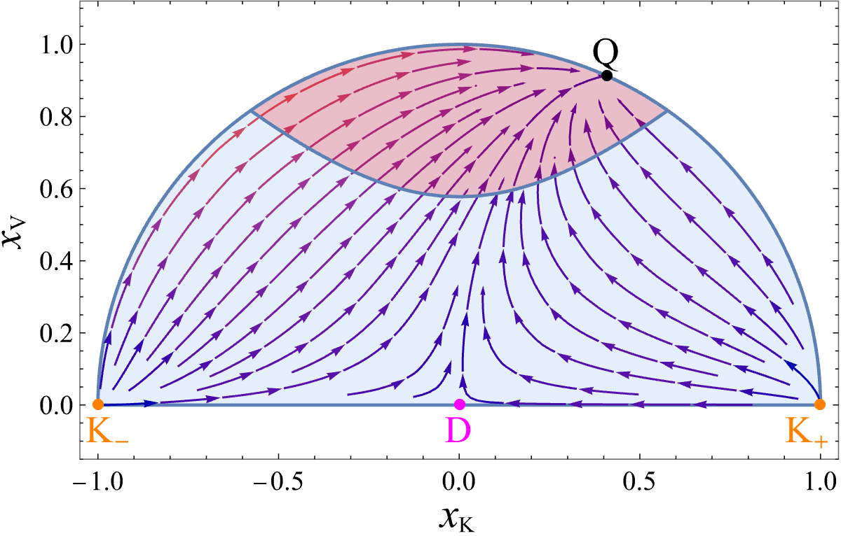
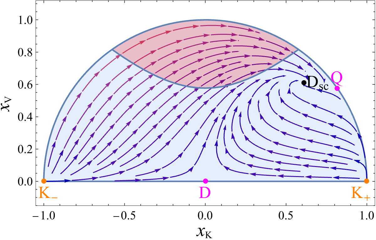
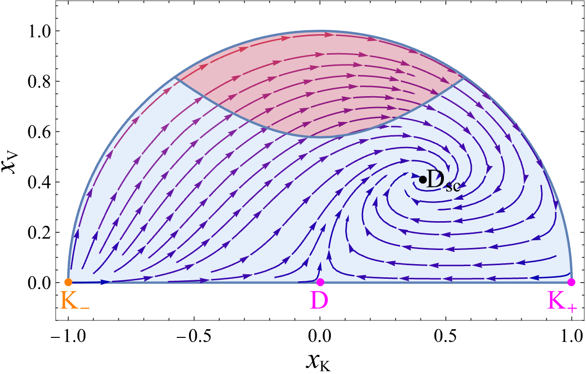
Figure 2: The phase space of $x_{\mathrm{K}}$ and $x_{\mathrm{V}}$ with $\lambda=1$ (the upper subfigure), $\lambda=2$ (the middle subfigure), and $\lambda=3$ (the bottom subfigure). Here we assume $x_{\mathrm{r}}=0$ to reduce the phase space to two dimensions. The fixed points listed in Table 1 are plotted, with yellow, magenta, and black representing stable, saddle, and unstable fixed points, respectively. Each streamline represents the evolution of the Universe under different initial conditions. The red region identifies accelerated expansion. It is clear that the scaling solution $\mathrm{D}_{\mathrm{sc}}$ is not in the accelerated expansion region.

Point R (D) is a radiation (dust) dominated solution and is able to describe the corresponding dominating epoch. Point $\mathrm{R}_{\mathrm{sc}}$ ($\mathrm{D}_{\mathrm{sc}}$) is the scaling solution [79, 82] for the ratio $\Omega_{\mathrm{q}}/\Omega_{\mathrm{r}}$ ($\Omega_{\mathrm{q}}/\Omega_{\mathrm{d}}$) is a non-zero constant, which can be used to hide the presence of the scalar field in the cosmic evolution, at least at the background level. The scaling solution must satisfy the condition $\lambda^{2}>3(1+w_{\mathrm{m}})$ in order to ensure that $\Omega_{\mathrm{q}}<1$. Since $w_{\mathrm{eff}}=w_{\mathrm{m}}$ and usually $0<w_{\mathrm{m}}<1$, scaling solution usually does not describe the cosmic acceleration (unless for a double exponential potential [83] and some related others [84, 85, 86]). Notice that the scaling solution returns to the corresponding dominated solution in the limit $\lambda\to\infty$.

Points $\mathrm{K}_{\pm}$ represent solutions dominated by a scalar field but are unable to account for the accelerating expansion due to the wrong EOS parameter. Hence, the only fixed point that represents the present cosmic epoch is the point Q, and the cosmic acceleration is realized if $\lambda^{2}<2$. As a result, the evolution of the Universe is consistent with the trajectory $\mathrm{R}\to\mathrm{D}\to\mathrm{Q}$.

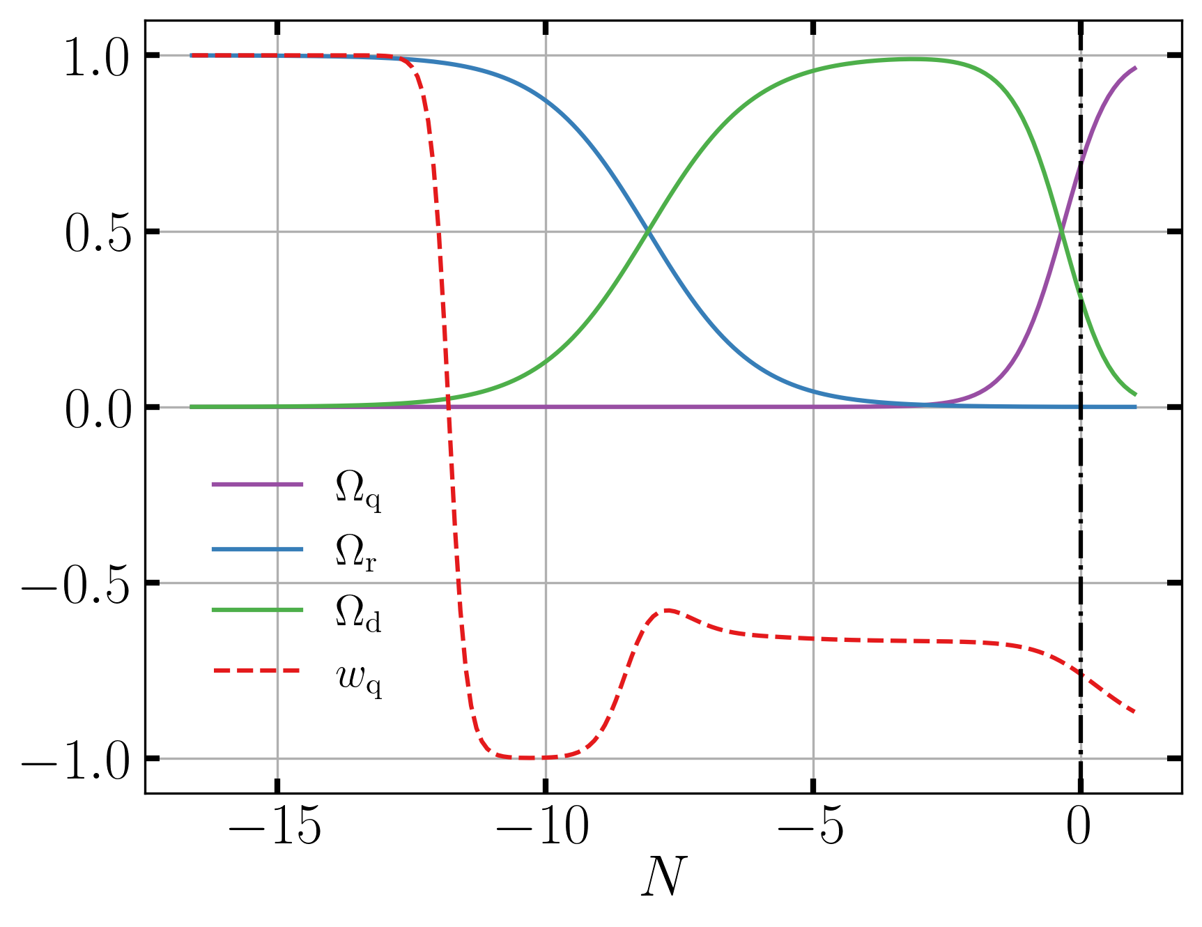
Figure 3: Evolution of $\Omega_{\mathrm{r}}$, $\Omega_{\mathrm{d}}$, $\Omega_{\mathrm{q}}$, and $w_{\mathrm{q}}$ for the potential $V(\phi)=M^{5}/\phi$ versus the $\rme$-folding time. The vertical dashed line denotes the present cosmological time, and the present values $\Omega_{\mathrm{d}}\simeq 0.3$ and $\Omega_{\mathrm{q}}\simeq 0.7$ are achieved. Here the complete curve of $w_{\mathrm{q}}$ is plotted, though it is literally no longer considered as quintessence when $w_{\mathrm{q}}>-1/3$. The solution enters the tracking regime in which the field energy density tracks the background fluid density. The initial conditions are chosen from [87].

If $\lambda$ is not a constant, we have to consider an additional equation

$$\frac{\rmd\lambda}{\rmd N}=-\sqrt{6}\lambda^{2}(\Gamma-1)x_{\mathrm{K}},$$ (3.35al)

where

$$\Gamma\equiv V\frac{\rmd^{2}V}{\rmd\phi^{2}}\left(\frac{\rmd V}{\rmd\phi}\right)^{-2}.$$ (3.35am)

In this scenario, the fixed points obtained in the case of a constant $\lambda$ can be considered as “instantaneous” fixed points that change over time [88, 89], if assuming that the time scale for the variation of $\lambda$ is significantly shorter than $H^{-1}$, the time scale that produces significant changes in the scale of the Universe.

The possibility of a transition from the fixed point $\mathrm{D}_{\mathrm{sc}}$ to Q arises when $\lambda$ decreases over time. If the condition $\Gamma>1$ is satisfied, the absolute value of $\lambda$ decreases towards $0$. This means that the solutions finally approach the accelerated instantaneous point Q even if $\lambda^{2}>2$ during radiation and matter domination. The condition $\Gamma>1$ is the so-called tracking condition under which the field density eventually catches up with that of the background fluid, and a tracking solution characterized by

$$\Omega_{\mathrm{q}}\simeq\frac{3(1+w_{\mathrm{q}})}{\lambda^{2}}$$ (3.35an)

is called a tracker [90]. Figure 3 shows the evolution of each components of a tracking solution. If $\Gamma$ varies slowly in time, the EOS parameter of quintessence is nearly constant during the matter domination and radiation domination periods [90, 91],

$$w_{\mathrm{q}}\simeq w_{\mathrm{q}}^{\rmi}=\frac{w_{\mathrm{m}}-2(\Gamma-1)}{2\Gamma-1}.$$ (3.35ao)

The fact that $w_{\mathrm{q}}<w$ results in a slower decrease of the quintessence energy density compared to the fluid energy density, and ultimately it leads to an attainable value of $\Omega_{\mathrm{q}}=1$. From Equation (3.35an), $w_{\mathrm{q}}$ is $-1+\lambda^{2}/3$ in the scalar field dominated epoch, which corresponds to the stable fixed point Q as long as $\lambda<3(1+w_{\mathrm{m}})$. The tracker fields correspond to attractor-like solutions, wherein the field energy density tracks the background fluid density across a wide range of initial conditions [74]. This implies that the energy density of quintessence does not necessarily need to be significantly smaller than that of radiation or matter in the early Universe, unlike in the cosmological constant scenario. Consequently, this offers a potential solution to alleviate the coincidence problem. Another benefit of the tracker solution is that it does not require the introduction of a new mass hierarchy in fundamental parameters [74].

In contrast to the tracking solution where $\Gamma>1$, if $\lambda$ gradually increases over time, the accelerated phase of the Universe is limited at late times because the energy density of the scalar field becomes negligible compared to that of the background fluid.

3.2 Cosmological Boundary

3.2.1 Phantom Dark Energy.

The EOS parameter for the cosmological constant, $w_{\Lambda}=-1$, is referred to as the cosmological boundary, for the reason not only distinguishing between the rates of accelerating expansion, whether slower or faster than exponential, but also marking the point where perturbation divergence occurs [92]. A canonical scalar field, when treated as a perfect fluid, is bound by an EOS parameter within the range $(-1,1)$. However, current observations suggest the possibility of the equation of state parameter of dark energy being smaller than $w_{\Lambda}$, a scenario even favored by the data [93, 94, 95, 10].

The phantom dark energy model was proposed as a complement to the canonical quintessence model [96], offering a super-accelerating phase, the expansion faster then exponential. This can be achieved by substituting the quintessence action with an alternative one:

$$S_{\mathrm{p}}[g^{\mu\nu},\phi]=\int\rmd^{4}x\sqrt{-g}\mathcal{L}_{\mathrm{p}}=\int d^{4}x\sqrt{-g}\left[\frac{1}{2}g^{\mu\nu}\partial_{\mu}\phi\partial_{\nu}\phi-V(\phi)\right].$$ (3.35ap)

The EOS parameter of the phantom field is

$$w_{\mathrm{p}}\equiv\frac{p_{\mathrm{p}}}{\rho_{\mathrm{p}}}=\frac{\dot{\phi}^{2}+2V(\phi)}{\dot{\phi}^{2}-2V(\phi)},$$ (3.35aq)

then one has $w_{\mathrm{p}}>1$ for the kinetic dominated regime ($\dot{\phi}^{2}/2>V$) and $w_{\mathrm{p}}<-1$ for the potential dominated regime ($V>\dot{\phi}^{2}/2$).

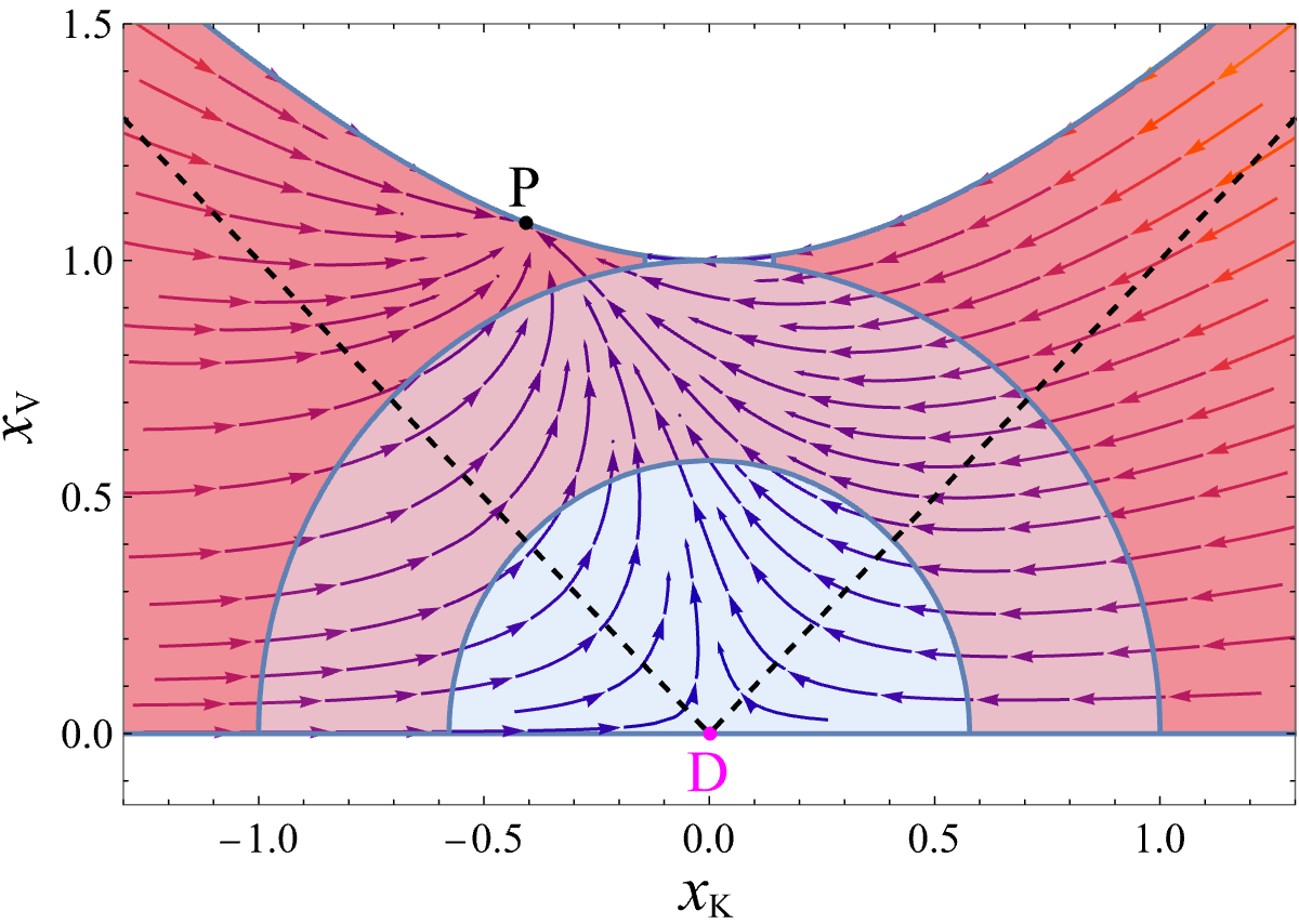
Figure 4: The phase space of $x_{\mathrm{K}}$ and $x_{\mathrm{V}}$ with value $x_{\mathrm{r}}=0$ and $\lambda=1$. The magenta saddle fixed point D represents the matter domination, while the black stable point P represents the phantom dominated stage. Each streamline represents the evolution of the Universe under different initial conditions. The light red region shows where Universe undergoes a standard accelerated expansion $-1<w_{\mathrm{eff}}<-1/3$, while the dark red region identifies expansion faster then exponential. The two green dashed lines correspond to $x_{\mathrm{V}}=\pm x_{\mathrm{K}}$ where the phantom EOS parameter diverges.

The choice of the same expansion normalised variables (3.29) also closes the system if the exponential potential (3.23) is considered. Hence, the analogous analysis can be transplanted for phantom models. Figure 4 shows the phase space of a phantom dark energy Universe with $w_{\mathrm{m}}=0$ (a different $w_{\mathrm{m}}\in[0,\frac{1}{3}]$ doesn’t alter qualitative descriptions below). Only two fixed points exist in the system: one is the saddle point D, where the Universe contains only matter, and the other is the stable state P, representing a phantom dominated attractor. A heteroclinic orbit connecting point D to point P would represent the late time translation from matter to phantom domination. On the way to the attractor, the expanding solution for the scalar field will be

$$a(t)\propto(t_{\infty}-t)^{-2/\lambda^{2}},$$ (3.35ar)

ultimately leading to the occurrence of the “Big Rip” singularity within a finite proper time $t_{\infty}$ [97, 98]. A potential bound from above is necessary to suppress this singularity, since the phantom field rolls up the potential and subsequently converge towards $w_{\mathrm{p}}=-1$ as the field stabilizes at the maximum of potential [99, 100].

Quantum instability always arises in phantom models due to the flipped sign of the kinetic term. Once the phantom quanta interact with other fields, even though gravity, there will be an instability of the vacuum because energy is no longer bound from below [99, 101]. Moreover, phantom models are problematic at the classical level because a strongly anisotropic CMB background is expected unless the Lorentz symmetry is broken for the phantom at an energy scale lower than 3 MeV [101]. Last but not least, the phantom model with an exponential potential fails to address the coincidence problem and suffers from the fine-tuning of initial condition. Consequently, the inclusion of sophisticated potentials and matter fluids beyond the range of $[0,\frac{1}{3}]$ have to be considered [102, 103].

3.2.2 Cross the Cosmological Boundary.

The EOS parameters for dark energy in both the quintessence and phantom models are confined to opposite sides of the cosmological boundary, preventing them from crossing over into each other’s domain. A no-go theorem indeed confirms this, stating as follows [104]: for the theory of dark energy in the FLRW Universe described by a single fluid or a single scalar field $\phi$ with a Lagrangian $\mathcal{L}=\mathcal{L}(\phi,\partial_{\mu}\phi\partial^{\mu}\phi)$, which minimally coupled to Einstein gravity, its EOS $w_{\mathrm{de}}$ cannot across the cosmological constant boundary.

In a scenario where gravity is still governed by general relativity, additional degrees of freedom are necessary to enable dark energy to effectively traverse the boundary. The quintom model was proposed as a multi-field model incorporating a quintessence-like field and a phantom-like field [105, 106],

$$S_{\mathrm{qp}}[g^{\mu\nu},\phi_{\mathrm{q}},\phi_{\mathrm{p}}]=\int\rmd^{4}x\sqrt{-g}\mathcal{L}_{\mathrm{qp}}\left[-\frac{1}{2}g^{\mu\nu}\partial_{\mu}\phi_{\mathrm{q}}\partial_{\nu}\phi_{\mathrm{q}}+\frac{1}{2}g^{\mu\nu}\partial_{\mu}\phi_{\mathrm{p}}\partial_{\nu}\phi_{\mathrm{p}}-V(\phi_{\mathrm{q}},\phi_{\mathrm{p}})\right].$$ (3.35as)

The energy density, pressure and the corresponding EOS parameter of the quintom model are

$$\rho_{\mathrm{de}}=\frac{1}{2}\dot{\phi}_{\mathrm{q}}^{2}-\frac{1}{2}\dot{\phi}_{\mathrm{p}}^{2}+V(\phi_{\mathrm{q}},\phi_{\mathrm{p}}),$$ (3.35at)

$$p_{\mathrm{de}}=\frac{1}{2}\dot{\phi}_{\mathrm{q}}^{2}-\frac{1}{2}\dot{\phi}_{\mathrm{p}}^{2}-V(\phi_{\mathrm{q}},\phi_{\mathrm{p}}),$$ (3.35au)

$$w_{\mathrm{de}}\equiv\frac{p_{\mathrm{qp}}}{\rho_{\mathrm{qp}}}=\frac{\dot{\phi}_{\mathrm{q}}^{2}-\dot{\phi}_{\mathrm{p}}^{2}-2V(\phi_{\mathrm{q}},\phi_{\mathrm{p}})}{\dot{\phi}_{\mathrm{q}}^{2}-\dot{\phi}_{\mathrm{p}}^{2}+2V(\phi_{\mathrm{q}},\phi_{\mathrm{p}})}.$$ (3.35av)

It is clear that $w_{\mathrm{qp}}\gtrless-1$ if $\dot{\phi}_{\mathrm{q}}\gtrless\dot{\phi}_{\mathrm{p}}$ and the cosmological constant scenario is recovered when $\dot{\phi}_{\mathrm{q}}=\dot{\phi}_{\mathrm{p}}$.

The potential $V(\phi_{\mathrm{q}},\phi_{\mathrm{p}})$ for non-interacting scalar fields can be generally written as

$$V(\phi_{\mathrm{q}},\phi_{\mathrm{p}})=V_{\mathrm{q}}(\phi_{\mathrm{q}})+V_{\mathrm{p}}(\phi_{\mathrm{p}}),$$ (3.35aw)

where $V_{\mathrm{q}}(\phi_{\mathrm{q}})$ and $V_{\mathrm{p}}(\phi_{\mathrm{p}})$ are arbitrary self-interacting potentials for the quintessence and phantom respectively. In such case, the two scalar field can be treated exactly as if they were single models. Due to the fact that $w_{\mathrm{p}}<w_{\mathrm{q}}$, the Universe will eventually evolve to a stage where phantom dominates $w_{\mathrm{eff}}=w_{\mathrm{de}}\leq-1$. The $w_{\mathrm{de}}$ across the cosmological boundary from above to below if the matter dominated epoch is followed by a temporary quintessence dominated stage [106, 107, 108]. If future observations will constrain the EOS parameter of dark energy to be below $-1$ today but above $-1$ in the past, then the quintom scenario of is arguably the simplest framework where such a situation can arise.

Unfortunately, neither the coupled nor the uncoupled quintom models seem to solve the cosmic coincidence problem and the fine-tuning of initial conditions simultaneously, not to mention the fundamental problems associated with the ghost field. Furthermore, couplings between kinetic terms and scalar fields, like $\partial_{\mu}\phi_{\mathrm{q}}\partial^{\mu}\phi_{\mathrm{p}}$ [109] and the so-called hessence dark energy model [110, 111, 112] are investigated as well. Finally, theories beyond general relativity, such as those incorporating higher curvature terms and non-minimally coupled scalar fields between gravity or matter, can also cross the cosmological boundary without encountering negative kinetic energy and the associated quantum instability, as discussed in 4.3.3.

3.3 Non-canonical Kinetic Term

In the preceding sections, some simplest dynamical dark energy models are introduced, providing as much detail as possible regarding their evolution. Here we briefly review dark energy models from scalar fields with modified kinetic terms, which hold significant potential for addressing those problems of $\Lambda$CDM model at once.

3.3.1 k-essence.

A scalar field model of dark energy with a modified kinetic term is the so-called kinetically driven essence, or k-essence for simplicity. The initial focus of the k-essence was on its application to inflation [113], and numerous theoretical models, such as low energy effective string theory [114], ghost condensate [115], tachyon [116, 117], and Dirac-Born-Infeld (DBI) theory, [118, 119] can be classified under this dark energy model.

The action of the k-essence dark energy model is given by [113]

$$S[g^{\mu\nu},\phi,\Psi_{\mathrm{m}}]=S_{\mathrm{EH}}[g^{\mu\nu}]+\int\rmd^{4}x\sqrt{-g}P(\phi,X)+S_{\mathrm{m}}[g^{\mu\nu},\Psi_{\mathrm{m}}],$$ (3.35ax)

where $P(\phi,X)$ is an arbitrary function of a scalar field $\phi$ and its kinetic energy

$$X\equiv-\frac{1}{2}g^{\mu\nu}\partial_{\mu}\phi\partial_{\nu}\phi.$$ (3.35ay)

The k-essence model can achieve accelerated expansion solely through kinetic energy, even in the absence of a potential [120, 121], distinguishing it from models with canonical kinetic energy.

The energy-momentum tensor of the k-essence is given by

$$T^{\mathrm{k}}_{\mu\nu}=-\frac{2}{\sqrt{-g}}\frac{\delta(\sqrt{-g}P)}{\delta g^{\mu\nu}}=P_{X}\partial_{\mu}\phi\partial_{\nu}\phi+g_{\mu\nu}P,$$ (3.35az)

where the subscript $X$ of function $P$ represents the partial derivative with respect to $X$. Comparing with the energy-momentum tensor of a perfect fluid (2.4), we have the pressure and energy density of the k-essence,

$$p_{\mathrm{k}}=P,$$ (3.35ba)

$$\rho_{\mathrm{k}}=2XP_{X}-P,$$ (3.35bb)

with the 4-velocity $u_{\mu}=\partial_{\mu}\phi/\sqrt{2X}$. If $P$ only depends on $\phi$, we obtain $p_{\mathrm{k}}=-\rho_{\mathrm{k}}$, which corresponds to general relativity with the cosmological constant. If $P$ solely depends on $X$, we have $\rho_{\mathrm{k}}=\rho_{\mathrm{k}}(X)$. Hence, $\rho_{\mathrm{k}}$ can be rearranged to give $p_{\mathrm{k}}=p_{\mathrm{k}}(\rho_{\mathrm{k}})$, which is the EOS for an isentropic fluid. In the general case where $p_{\mathrm{k}}=P(\phi,X)$, the hydrodynamical analogy is still useful, and the EOS parameter is acquired directly,

$$w_{\mathrm{k}}\equiv\frac{p_{\mathrm{k}}}{\rho_{\mathrm{k}}}=\frac{P}{2XP_{X}-P},$$ (3.35bc)

and $w_{\mathrm{k}}$ approaches to $-1$ if the condition $|XP_{X}|\ll|P|$ is satisfied.

A non-canonical scalar field Lagrangian will in general introduce theoretical problems at both the quantum and classical levels. Hence, the selection of function $P$ has limitations. The propagation sound speed $c_{\mathrm{s}}^{\mathrm{k}}$ of the k-essence field is given by [122],

$$\big{(}c^{\mathrm{k}}_{\mathrm{s}}\big{)}^{2}=\frac{\partial p_{k}/\partial X}{\partial\rho_{k}/\partial X}=\frac{P_{X}}{P_{X}+2XP_{XX}},$$ (3.35bd)

which should be a positive number. Furthermore, due to the positive definiteness of the Hamiltonian [123], both the denominator $\xi_{1}$ and the numerator $\xi_{2}$ of $\big{(}c^{\mathrm{k}}_{\mathrm{s}}\big{)}^{2}$ in Equation (3.35bd) should be positive. To be in accordance with the principle of causality, $c_{\mathrm{s}}^{\mathrm{k}}$ is considered favorable if it does not exceed the speed of light which gives $P_{XX}\geq 0$; however, see Ref. [124].

On account of the unknown dependence upon the arbitrary function $P(\phi,X)$, it is too complicated to directly study with dynamical systems techniques. Therefore, to study their dynamics and evolution, k-essence are typically divided into several classes [78]:

$$\mathrm{Class\ I:}\quad P(\phi,X)=XG(Y),\quad Y=\frac{X}{V(\phi)},$$ (3.35be)

$$\mathrm{Class\ II:}\quad P(\phi,X)=K(\phi)\tilde{P}(X),$$ (3.35bf)

$$\mathrm{Class\ III:}\quad P(\phi,X)=F(X)-V(\phi),$$ (3.35bg)

where $G$, $K$, $\tilde{P}$, $F$ and $V$ are functions of their own arguments. It is worth noting that a model can be classified into one of two classes, as seen with the quintessence model, or it may not fit into either category, as exemplified by the DBI model.

The first class of k-essence exhibits a deep connection with scaling solutions that are of great relevance for the cosmic coincidence problem. It has been proved that [123] scaling solutions appear in k-essence models only if a Lagrangian of the type (3.35be) is assumed with $V(\phi)\propto\rme^{-\lambda\phi/M_{\mathrm{Pl}}}$. Further research indicated that dark energy late-time solutions are invariably unstable in the presence of a scaling solution, unless they belong to the phantom type, even with a coupling to the matter sector [125, 126]. Note that the quintessence exhibits scaling solutions because it corresponds to $G(Y)=1-1/Y$.

Unlike the Class I, the second class is intriguing for its tracking solutions. It has been shown that tracking solutions naturally appear for the models (3.35bf) during the radiation dominated era, and a cosmological-constant-like behavior shortly after the transition to matter domination were put forward, which claims to have solved the coincidence problem without fine-tuning the parameters [127, 128]. However, a singularity associated with a diverging sound speed is present in such models [129], so that it cannot arise as a low-energy effective field theory of a causal, consistent, high-energy theory. Moreover, the Lagrangians in these models are hard to construct in the framework of particle physics.

The third class (3.35bg) has a non-canonical kinetic term appears together with a standard self-interacting potential for the scalar field. The famous (dilatonic) ghost condensate is usually considered a subclass of this kind, which is simply recommended in next Section 3.3.2. One interesting thing is that some special functions $F(X)$ and $V(\phi)$ produce scaling solutions, even if the Lagrangian cannot be written in the form of Class I [130].

3.3.2 (Dilatonic) Ghost Condensate.

The quintessence and phantom models, as special cases of k-essence, have

$$P(\phi,X)=\epsilon X-V(\phi),$$ (3.35bh)

where $\epsilon=\pm 1$ represents quintessence and phantom respectively.

The denominator and numerator of propagation sound speed are $\xi_{1}=\xi_{2}=\epsilon$, indicating the phantom model is unstable. The instabilities come form the perturbation level, where the gradient energy plays an important role. Therefore, one approach is to introduce a background action resembling that of a ghost, allowing the spatial gradient terms to address the instability issue. To implement the idea, Arkani-Hamed et al. [115] proposed an effective field theory of a rolling ghost, which can be conceptualized as an infrared modification of gravity. They termed this modification as ghost condensate with the arbitrary function taking the form

$$P(\phi,X)=-X+\frac{X^{2}}{M^{4}},$$ (3.35bi)

where $M$ is a constant having a dimension of mass. This model was later generalized to a modified version as

$$P(\phi,X)=-X+\frac{X^{2}}{M^{4}}\exp{\left(\frac{\lambda\phi}{M_{\mathrm{Pl}}}\right)},$$ (3.35bj)

which is called dilatonic ghost condensate model [123].

Here we briefly introduce the cosmic evolution of dilatonic ghost condensate dark energy model. The pressure, energy density and the corresponding EOS parameter are

$$p_{\mathrm{dGC}}=-X+\frac{X^{2}}{M^{4}}\rme^{\lambda\phi},$$ (3.35bk)

$$\rho_{\mathrm{dGC}}=-X+\frac{3X^{2}}{M^{4}}\rme^{\lambda\phi},$$ (3.35bl)

$$w_{\mathrm{dGC}}\equiv\frac{p_{\mathrm{dGC}}}{\rho_{\mathrm{dGC}}}=\frac{1-\rme^{\lambda\phi}X/M^{4}}{1-3\rme^{\lambda\phi}X/M^{4}},$$ (3.35bm)

where $M_{\mathrm{Pl}}=1$ is used for briefness. Quantum stability necessitates $\rme^{\lambda\phi}X/M^{4}\geq 1/2$, resulting in the EOS parameter lying within the range $-1\leq w_{\mathrm{dGC}}<1/3$. In particular the de Sitter solution $w_{\mathrm{dGC}}=-1$ is realized at $X=M^{4}e^{-\lambda\phi}/2$. Then it is possible to explain the present cosmic acceleration for $M\sim 10^{-3}\;\mathrm{eV}$ in ghost condensate model as $\rho_{\mathrm{GC}}=-p_{\mathrm{dGC}}=M^{4}/4$ at the de Sitter point. Hence, the (dilatonic) ghost condensate is another example of accelerated expansion that can be generated without the assistance of a potential.

By adjusting the selection of dynamic variables to [87]

$$x_{\mathrm{K}}\equiv\frac{\dot{\phi}}{\sqrt{6}H},\quad x_{\mathrm{M}}\equiv\frac{\dot{\phi}^{2}\rme^{\lambda\phi}}{2M^{4}},\quad x_{\mathrm{r}}\equiv\frac{\sqrt{\rho_{\mathrm{r}}}}{\sqrt{3}H}.$$ (3.35bn)

we can get the autonomous system describing the dilatonic ghost condensate model. There always exists a stable point describing accelerated expansion toward which the Universe evolves, as long as $0\leq\lambda<\sqrt{6}/3$. The corresponding sound speed is in the range $0\leq c_{\mathrm{s}}^{\mathrm{dGC}}<1/3$, which means this model does not violate causality. The EOS parameter of this future attractor is [87]

$$w_{\mathrm{eff}}=w_{\mathrm{dGC}}=\frac{\lambda^{2}f(\lambda)-8}{3\lambda^{2}f(\lambda)+8},\quad f(\lambda)=1+\sqrt{1+\frac{16}{3\lambda^{2}}},$$ (3.35bo)

which suggests that the ghost condensate behaves like a cosmological constant in dynamics during the final stage of cosmic evolution.

3.3.3 Unified Dark Matter and Dark Energy.

The temptation to unify dark matter and dark energy into a single entity has occurred to many cosmologists almost from the beginning, in order to solve two big dark sector problems at once. Both a fluid and a scalar field are attempted to represent dark matter and dark energy at the same times [131, 132, 133, 134]. Here we simply introduce a kind of k-essence model that is regarded as dark matter and dark energy simultaneously.

The Lagrangian of a such k-essence model with only a kinetic term is [132]

$$P(\phi,X)=-F_{0}+F_{2}(X-X_{0})^{2},$$ (3.35bp)

where $F_{0}$ and $F_{2}$ are constants. Notice that there is an extremum $X_{0}$ of the kinetic energy, around which the pressure and energy density of k-essence are approximately

$$p_{\mathrm{k}}\simeq-F_{0},$$ (3.35bq)

$$\rho_{\mathrm{k}}\simeq F_{0}+4F_{2}X_{0}(X-X_{0}).$$ (3.35br)

Furthermore, by substituting $X=X_{0}(1+\varepsilon a^{-3})$ with $0<\varepsilon a^{-3}\ll 1$ ($\varepsilon$ being a constant), the solution to the continuity equation around $X_{0}$ yields the EOS parameter

$$w_{\mathrm{k}}=-\left(1+\frac{4F_{2}}{F_{0}}X_{0}^{2}\varepsilon a^{-3}\right)^{-1}.$$ (3.35bs)

It is possible to realize $w_{\mathrm{k}}\simeq 0$ during the matter domination provided that the condition $4F_{2}X_{0}^{2}/F_{0}\gg 1$ is satisfied, while $w_{\mathrm{k}}$ approaches the de Sitter value $-1$ at late time due to $\varepsilon a^{-3}\to 0$. This specific model does not suffer from the problem of stability or causality if $X>X_{0}$, rendering it a more reliable unified model.

3.4 Interacting Dark Energy Model

Typically, the dark energy models are based on scalar fields minimally coupled to the gravity, and do not implement the explicit coupling of the field to background matter, as illustrated by the models introduced above. However, there is no fundamental reason for this assumption in the absence of an underlying symmetry supposed to suppress the coupling, in particular the dark sector that we barely no nothing about from a microscopic and dynamical field theory perspective. Although the interaction between dark energy and normal matter particles are heavily restricted by observations [135, 38], this is not the case for dark matter particles, and the neglect of this potential interaction of dark components may result in misinterpretations of observational data. In fact, the study of the interaction between dark energy and dark matter is getting more promising recently, for the possible solution to the coincident problem and tensions in $\Lambda$CDM models.

3.4.1 Phenomenological Description.

Since there is no established approach from first principles that can specify the form of coupling between dark energy and dark matter, dark matter could manifest as either bosonic or fermionic particles, adhering to either the standard model or extending beyond it. Likewise, dark energy could be conceptualized as a fluid, a field, or in other forms. Constructing phenomenological models initially, grounded in intuition and experience, is consistently beneficial. These models can then be rigorously tested against diverse observational data.

The interaction between dark matter and dark energy is described by following modified conservation equations,

$$\dot{\rho}_{\mathrm{dm}}+3H\rho_{\mathrm{dm}}=Q,$$ (3.35bt)

$$\dot{\rho}_{\mathrm{de}}+3H(1+w_{\mathrm{de}})\rho_{\mathrm{de}}=-Q,$$ (3.35bu)

where $Q$ is termed the interacting kernel and its sign determines the direction of the energy flux. Specifically, energy transfers from dark energy to dark matter when $Q>0$ and the transmission reverses when $Q<0$. The original model is restored if the interaction is “turned off”.

In order to illustrate how interaction between the dark components acts on cosmological dynamics, consider the time evolution of the radio $r\equiv\rho_{\mathrm{dm}}/\rho_{\mathrm{de}}$,

$$\dot{r}=\frac{\rho_{\mathrm{dm}}}{\rho_{\mathrm{de}}}\left(\frac{\dot{\rho}_{\mathrm{dm}}}{\rho_{\mathrm{dm}}}-\frac{\dot{\rho}_{\mathrm{de}}}{\rho_{\mathrm{de}}}\right)=-3\Gamma Hr,\quad\Gamma=-w_{\mathrm{de}}-\frac{1+r}{\rho_{\mathrm{dm}}}\frac{Q}{3H}.$$ (3.35bv)

It is not difficult to observe that the interaction kernel should be the product of an energy density and a term with an inverse time dimension. Additionally, it is natural to assume that the kernel depends solely on relevant dynamical quantities (such as $\rho_{\mathrm{dm}}$, $\rho_{\mathrm{de}}$ and $a$) and possibly their derivatives. The simplest cases can be the following kernels

$$Q\supset\xi_{1}\rho_{\mathrm{dm}}H,\xi_{2}\rho_{\mathrm{de}}H,\xi_{3}\dot{\rho}_{\mathrm{dm}},\xi_{4}\dot{\rho}_{\mathrm{de}},\cdots$$

and their linear combinations. Other forms of interaction kernel including nonlinearity and a lot of complexity are summarized in review papers like [136, 137].

Now, let us consider the case $Q=3H(\xi_{1}\rho_{\mathrm{dm}}+\xi_{2}\rho_{\mathrm{de}})$ and examine how the interacting dark energy model can resolve the coincidence problem. For this particular kernel,

$$\Gamma=-w_{\mathrm{de}}-\frac{(1+r)(\xi_{1}r+\xi_{2})}{r},$$ (3.35bw)

and the stationary solutions are obtained imposing $r_{\mathrm{s}}\Gamma(r_{\mathrm{s}})=0$, which gives ($\xi_{1}\neq 0$)

$$r_{\mathrm{s}}^{\pm}=-\frac{w_{\mathrm{de}}+\xi_{1}+\xi_{2}\pm\sqrt{(w_{\mathrm{de}}+\xi_{1}+\xi_{2})^{2}-4\xi_{1}\xi_{2}}}{2\xi_{1}}.$$ (3.35bx)

The coincidence problem is completely solved if one of the above roots $r_{\mathrm{s}}^{\pm}$ is the future attractor of the system. Moreover, the evolution of the Universe should gradually approach the attractor from above, implying that the ratio of matter to dark energy decreases over time. In the special case $\xi_{1}=\xi_{2}=\xi$, the larger root $r_{\mathrm{s}}^{-}$ is a past attractor while the smaller root $r_{\mathrm{s}}^{+}$ is a future attractor [138, 139]. As Universe expands, $r(t)$ will evolve from $r_{\mathrm{s}}^{-}$ to the stable solution $r_{\mathrm{s}}^{+}$ avoiding the coincidence problem if $r_{\mathrm{s}}^{+}\sim 3/7$. If $\xi_{2}=0$, the system still retains a past attractor $r_{s}^{+}$ with no future attractor ($r_{\mathrm{s}}^{-}=0$ in this case). However, the variation is $|(\dot{r}/r)_{0}|<H_{0}$, slower than in $\Lambda$CDM, which mitigates the coincidence problem [140]. As for the $\xi_{1}=0$ case, it is fortunate that the only fixed point $r_{\mathrm{s}}=-\xi_{2}/(w_{\mathrm{de}}+\xi_{2})$ is stable. Consequently, there is no more coincidence problem if we select $\xi_{2}\sim 0.3$ under the assumption of $w_{\mathrm{de}}=-1$. Figure 5 showing the phase space of this example will help understand the conclusion.

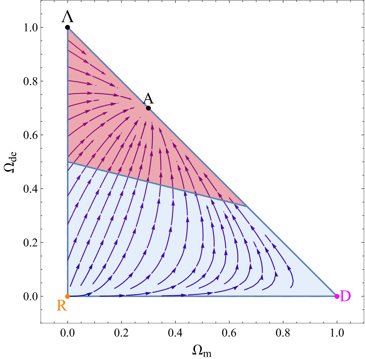
Figure 5: The diagram of $\Omega_{\mathrm{m}}$-$\Omega_{\mathrm{de}}$ with values $w_{\mathrm{de}}=-1$ and $\xi_{2}=0.3$ in the case where $Q=3\xi_{2}H\rho_{\mathrm{de}}$. The black point A is the only stable fixed point in the system representing the future attractor with $\Omega_{\mathrm{m}}=0.3$ and $\Omega_{\mathrm{de}}=0.7$. The black point $\Lambda$ is the future attractor of $\Lambda$CDM model with $\Omega_{\mathrm{m}}=0$ and $\Omega_{\mathrm{de}}=1$. The orange point R and magenta point D are unstable radiation domination and saddle matter domination respectively. Each streamline represents the evolution of the Universe under different initial conditions. The red region identifies accelerated expansion.

While the initial drive behind interacting dark energy models was to solve or alleviate the coincidence problem, their focus has recently shifted towards elucidating the disparity between the observed value of the Hubble constant derived from CMB data and the local measurements. The interacting dark energy model increases the proportion of late-time dark energy, directly boosting the Hubble expansion rate. Moreover, the reduction in dark matter entails an increase in the Hubble constant to uphold the physical ratio of dark matter energy density in accordance with CMB constraints. In addition, dark matter decaying into dark energy also reduces structure growth of matter at late time, thereby alleviating the $S_{8}$ problem. Consequently, the interacting dark energy model emerges as a multifaceted potential solution to the Hubble tension.

3.4.2 Coupled Scalar Fields.

If focusing our attention on dark energy in the form of quintessence, one has the coupled quintessence model with the modified Klein-Gordon equation

$$\ddot{\phi}+3H\dot{\phi}+\frac{\rmd V}{\rmd\phi}=-\frac{Q}{\dot{\phi}}.$$ (3.35by)

The basic kernel $Q\propto\rho_{\mathrm{dm}}\dot{\phi}$ naturally emerges in certain modified gravity theories (such as $f(R)$ gravity [141, 142]) in the Einstein frame, through which dynamics are introduced in Section 4.2.1.

In general, all aforementioned dark energy models can be generalized by introducing a coupling in the dark sector, following the same approach as with quintessence. The coupled phantom models with exponential potentials and frequently analyzed couplings demonstrate that scaling solutions cannot remain stable [27, 143], as is the case with quintessence. Therefore, they are unable to resolve the cosmic coincidence problem.

The situation is different for more general k-essence models. Scaling solutions typically exist in Lagrangians of the form $P(\phi,X)=Q^{2}(\phi)XG(XQ^{2}(\phi)\rme^{\lambda\phi/M_{\mathrm{Pl}}})$, where $Q(\phi)$ is the coupling function and $G$ an arbitrary function [126]. However, it has been demonstrated that an evolutionary trajectory capable of resolving the coincidence problem is prohibited due to the singularity associated with both dynamical variables and the sound speed [126]. As additional resources, the study of coupled tachyonic models can be found in [144, 145, 146], while coupled DBI scalar field models are discussed in [147, 148].

4 Scalar-Tensor Gravity

Physicists introduced dark energy to explain the accelerating phase of the Universe, but the nature of this bizarre substance is unknown and the validity has also been called into questions. Since the evidence for dark energy comes entirely from its gravitational effects, which are inferred assuming the validity of general relativity, the consideration of modifications to general relativity, such that the necessity of dark energy is obviated, is another rational approach [37]. In this section, we focus on the scalar-tensor gravity, one of the most studied modified theories of gravity.

4.1 Introduction to Scalar-Tensor Gravity

The central idea behind scalar-tensor gravity theory is the incorporation of a scalar field alongside the metric tensor field to participate in the gravitational interaction. This addition of the scalar field allows for variations in the strength of gravity over spacetime, opening up new avenues for understanding the fundamental forces of the Universe. Scalar-tensor theory has since evolved and been refined in various forms and models, becoming a focal point for research in cosmology, astrophysics, and fundamental physics [30].

The origins of scalar-tensor gravity can be traced back to the pioneering work in the mid-20th century. One of the earliest proponents of this theory was the German physicist Jordan [149], who in 1955 introduced the concept of a scalar field coupled to gravity as a means to unify gravity with electromagnetism. Moreover, it was Brans and Dicke who further developed and formalized the theory in 1961 [150], now known as the Brans-Dicke (BD) theory. The action for the theory is,

$$S_{\mathrm{BD}}[g^{\mu\nu},\Phi,\Psi_{\mathrm{m}}]=\int\rmd^{4}x\sqrt{-g}\left(\Phi\frac{R}{2\kappa}-\frac{\omega_{\mathrm{BD}}}{2\Phi}g^{\mu\nu}\partial_{\mu}\Phi\partial_{\nu}\Phi\right)+S_{\mathrm{m}}[g^{\mu\nu},\Psi_{\mathrm{m}}],$$ (3.35a)

where $w_{\mathrm{BD}}$ is the only parameter in the theory. Here we add a coefficient of $\frac{1}{2}$ to the Lagrangian of the gravitational part of the traditional BD theory. Shortly afterward, Bergmann [151] and Wagoner [152] separately generalized the action to

$$S_{\mathrm{J}}[g^{\mu\nu},\Phi,\Psi_{\mathrm{m}}]=\int\rmd^{4}x\sqrt{-g}\left[\Phi\frac{R}{2\kappa}-\frac{W(\Phi)}{2\Phi}g^{\mu\nu}\partial_{\mu}\Phi\partial_{\nu}\Phi-U(\Phi)\right]+S_{\mathrm{m}}[g^{\mu\nu},\Psi_{\mathrm{m}}]\,,$$ (3.35b)

by letting the coupling parameter $w_{\mathrm{BD}}$ be a function of the scalar field $W(\Phi)$ and adding a potential term $U(\Phi)$. The subscript “J” here represents the Jordan frame.

A suitable conformal transformation

$$g_{\mu\nu}\to g_{\mu\nu}^{*}=A^{-2}(\phi)g_{\mu\nu}$$ (3.35c)

is able to take us from the Jordan frame to the Einstein frame [153]. We denote the scalar field in the Einstein frame as $\phi$ instead of the field $\Phi$ in the Jordan frame. The action in the Einstein frame is

$$S_{\mathrm{E}}[g^{\mu\nu}_{*},\phi,\Psi_{\mathrm{m}}]=\int\rmd^{4}x\sqrt{-g_{*}}\left[\frac{R_{*}}{2\kappa_{*}}-\frac{1}{2}g_{*}^{\mu\nu}\partial_{\mu}\phi\partial_{\nu}\phi-V(\phi)\right]+S_{\mathrm{m}}[A^{-2}(\phi)g^{\mu\nu}_{*},\Psi_{\mathrm{m}}],$$ (3.35d)

where $\kappa_{*}=8\pi G_{*}$, and $G_{*}$ is a bare gravitational constant. The physical quantity marked with a star indicates that it is in the Einstein frame. The potential $V(\phi)$ in the Einstein frame is related to the potential $U(\Phi)$ in the Jordan frame by the rescaling function $A(\phi)$ as

$$V(\phi)=A^{4}(\phi)U(\phi).$$ (3.35e)

The gravity theory is usually not invariant under conformal transformation, including Einstein’s general relativity. A natural question arises: which conformal frame is physical? Unfortunately, as of now, the answer remains unknown. In the subsequent Section 4.2 and Section 4.3, the Einstein frame and Jordan frame are both considered, respectively. Cosmologies within these two frames are discussed as well in corresponding sections.

4.2 Einstein Frame: Coupled Quintessence

The canonical form of action (3.35d) is acquired if $A(\phi)$ satisfies

$$A^{2}(\phi)=\frac{\kappa}{\kappa_{*}\Phi},$$ (3.35f)

$$\alpha^{2}(\phi)=\frac{1}{2[2\kappa W(\Phi)+3]},$$ (3.35g)

where $\alpha(\phi)\equiv{\rmd\ln A}/{\rmd\phi}$. The relation between scalar fields $\Phi$ and $\phi$ in Jordan and Einstein frames is easily acquired from Equations (3.35f) and (3.35g), as

$$\frac{\rmd\phi}{\rmd\Phi}=\pm\frac{\sqrt{\kappa W(\Phi)+3/2}}{\Phi}.$$ (3.35h)

From now on, we will use the unit $\kappa=1$ for simplicity.

The equations of motion derived from action (3.35d) read

$$G_{\mu\nu}^{*}=\kappa_{*}(T^{*\mathrm{m}}_{\mu\nu}+T_{\mu\nu}^{*\phi}),$$ (3.35i)

$$\square_{*}\phi=\frac{\rmd V}{\rmd\phi}-\alpha T_{\mathrm{m}}^{*},$$ (3.35j)

where $T^{*}_{\mathrm{m}}\equiv g^{\mu\nu}_{*}T^{*\mathrm{m}}_{\mu\nu}$ is the trace of $T_{\mu\nu}^{*\mathrm{m}}$, and the energy-momentum tensors of the background fluid and the scalar field are

$$T^{*\mathrm{m}}_{\mu\nu}=-\frac{2}{\sqrt{-g_{*}}}\frac{\delta(\sqrt{-g_{*}}\mathcal{L}_{\mathrm{m}})}{\delta g_{*}^{\mu\nu}},$$ (3.35k)

$$T^{*\phi}_{\mu\nu}=\partial_{\mu}\phi\partial_{\nu}\phi-g^{*}_{\mu\nu}\left[\frac{1}{2}g^{\alpha\beta}_{*}\partial_{\alpha}\phi\partial_{\beta}\phi+V(\phi)\right].$$ (3.35l)

When $\alpha=0$, the field equations of scalar-tensor gravity in the Einstein frame, Equations (3.35i) and (3.35j), along with energy-momentum tensors in Equations (3.35k) and (3.35l), are in the same form of the field equations (3.3) and (3.4) and the energy-momentum tensors in Equations (3.5) and (3.6) for the quintessence model, respectively, so that the gravity is entirely described by the metric tensor. The modification of gravity comes from the direct coupling term $\alpha(\phi)T_{\mathrm{m}}^{*}$ in Equation (3.35j) between the fluid and the scalar field $\phi$. Hence, the local conservation of the energy-momentum tensor no longer holds in the Einstein frame, and it changes to

$$\nabla^{*}_{\mu}T^{\mu\nu}_{*\mathrm{m}}=\alpha(\phi)T_{\mathrm{m}}^{*}\nabla^{\nu}_{*}\phi.$$ (3.35m)

As a result, the test particle does not move along geodesics of $g^{*}_{\mu\nu}$ anymore, as if it suffers from a kind of “fifth force”. According to Equation (3.35m), the original quintessence model is recovered as $\alpha(\phi)$ vanishes, which corresponds to the case where the function $W(\Phi)$ in the Jordan frame diverges. In this subsection we discuss the results in the Einstein frame, and the star notation of physical quantity is omitted in the following part of this subsection for simplicity. But keep in mind that we are in the Einstein frame.

4.2.1 Dynamics of Coupled Quintessence.

The fact that the energy density of dark energy is of the same order as that of dark matter in the present Universe suggests that there may be some relation between them. Among various coupled dark energy models [80], the coupled quintessence includes an interaction between a scalar field $\phi$ and the dust matter—nonrelativistic matter whose pressure is zero—in the form [154, 155],

$$\nabla^{\mu}T_{\mu\nu}^{\phi}=-\alpha(\phi)T_{\mathrm{d}}\nabla^{\nu}\phi,\quad\nabla^{\mu}T^{\mathrm{d}}_{\mu\nu}=\alpha(\phi)T_{\mathrm{d}}\nabla^{\nu}\phi,$$ (3.35n)

where $T_{\mu\nu}^{\phi}$ and $T^{\mathrm{d}}_{\mu\nu}$ are the energy-momentum tensors of the scalar field and the dust. The coupling of the scalar field and radiation vanishes due to the vanishing trace of $T_{\mu\nu}^{\mathrm{r}}$, the energy-momentum tensor of the radiation. Generally speaking, the coupling strength $\alpha(\phi)$ between the scalar field and various components of the Universe is not necessarily uniform [156, 157, 158, 159], and the baryons are usually treated uncoupled to the scalar field to avoid an extra long-range force besides gravity.

We only consider the case where the coupling $\alpha$ is a constant and the potential is exponential for simplicity, then the Friedmann equations are Equations (3.9) and (3.10), which are the same as for the quintessence. However, the evolution of the dust and the scalar field obeys different equations

$$\dot{\rho}_{\mathrm{d}}+3H\rho_{\mathrm{d}}=\alpha\rho_{\mathrm{m}}\dot{\phi},$$ (3.35q)

$$\dot{\rho}_{\phi}+3H(\rho_{\phi}+p_{\phi})=-\alpha\rho_{\mathrm{m}}\dot{\phi},$$ (3.35r)

where $\rho_{\phi}$ and $p_{\phi}$ have already been shown in Equations (3.11) and (3.12).

Introducing the same expansion normalised variables $x_{\mathrm{K}}$, $x_{\mathrm{V}}$ and $x_{\mathrm{r}}$ defined in Equation (3.29), we have an altered differential equation

$$\frac{{\rmd}x_{\mathrm{K}}}{\rmd N}=-3x_{\mathrm{K}}+\frac{\sqrt{6}}{2}\lambda x_{\mathrm{V}}^{2}-x_{\mathrm{K}}\frac{1}{H}\frac{\rmd H}{\rmd N}-\frac{\sqrt{6}}{2}\alpha(1-x_{\mathrm{K}}^{2}-x_{\mathrm{V}}^{2}-x^{2}_{\mathrm{r}})$$ (3.35s)

for $x_{\mathrm{K}}$, while the equations for $x_{\mathrm{V}}$ and $x_{\mathrm{r}}$ do not change, so as the EOS parameters and density parameters defined in Section 3.1.3. Except for the fixed points in Table 1, additional ones of the coupled quintessence are listed in Table 2, and Figure 6 shows fixed points in the phase space with $\lambda=1$ and different coupling constant $\alpha$.

Table 2: Properties of additional fixed points for the coupled quintessence with a constant $\alpha$ and potential (3.23) [155, 87].

Fixed point	$(x_{\mathrm{K}},x_{\mathrm{V}},x_{\mathrm{r}})$	$\Omega_{\mathrm{r}}$	$\Omega_{\mathrm{d}}$	$\Omega_{\phi}$	$w_{\phi}$	$w_{\mathrm{eff}}$
$\mathrm{R}_{\mathrm{ex}}$	$\Big{(}-\frac{1}{\sqrt{6}\alpha},0,\frac{\sqrt{2\alpha^{2}-1}}{\sqrt{2}\alpha}\Big{)}$	$1-\frac{1}{2\alpha^{2}}$	$\frac{1}{3\alpha^{2}}$	$\frac{1}{6\alpha^{2}}$	$1$	$\frac{1}{3}$
$\mathrm{D}^{\prime}$	$\Big{(}-\frac{\sqrt{6}\alpha}{3},0,0\Big{)}$	$0$	$1-\frac{2\alpha^{2}}{3}$	$\frac{2\alpha^{2}}{3}$	$1$	$\frac{2\alpha^{2}}{3}$
$\mathrm{D}_{\mathrm{sc}}^{\prime}$	$\Big{(}\frac{\sqrt{6}}{2(\alpha+\lambda)},\frac{\sqrt{2\alpha^{2}+2\alpha\lambda+3}}{2(\alpha+\lambda)},0\Big{)}$	$0$	$\frac{\lambda^{2}+\alpha\lambda-3}{(\alpha+\lambda)^{2}}$	$\frac{\alpha^{2}+\alpha\lambda+3}{(q+\lambda)^{2}}$	$-\frac{\alpha(\alpha+\lambda)}{\alpha(\alpha+\lambda)+3}$	$-\frac{\alpha}{\alpha+\lambda}$

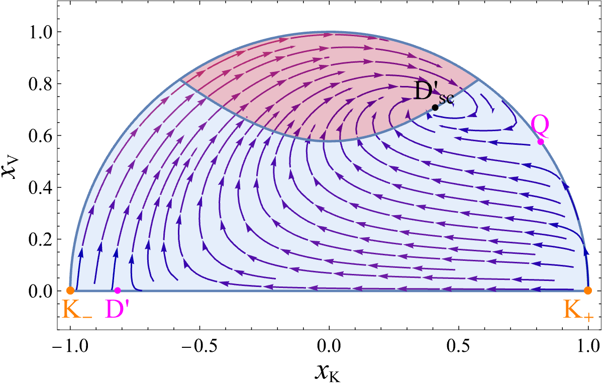
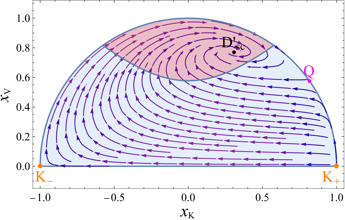
Figure 6: The phase space of $x_{\mathrm{K}}$ and $x_{\mathrm{V}}$ with $\alpha=0$ (the upper subfigure), $\alpha=1$ (the middle subfigure), and $\alpha=2$ (the bottom subfigure). Here we assume $x_{\mathrm{r}}=0$ and $\lambda=1$. The fixed points of coupled quintessence are plotted, with yellow, magenta, and black representing stable, saddle, and unstable fixed points, respectively. Each streamline represents the evolution of the Universe under different initial conditions. The red region identifies accelerated expansion. Each point on the curve $x_{\mathrm{K}}^{2}+x_{\mathrm{V}}^{2}=1$ corresponds to $\Omega_{\mathrm{q}}=1$. Since the future attractor $\mathrm{D}_{\mathrm{sc}}^{\prime}$ in the bottom subfigure lies in the red region but not on the semi-circle, it offers a solution to the coincidence problem.

In the coupled quintessence model, fixed point $\mathrm{D}^{\prime}$ ($\mathrm{D}_{\mathrm{sc}}^{\prime}$) replaces D ($\mathrm{D}_{\mathrm{sc}}$) in the uncoupled case, and $\mathrm{D}^{\prime}$ ($\mathrm{D}_{\mathrm{sc}}^{\prime}$) returns to D ($\mathrm{D}_{\mathrm{sc}}$) when the coupling $\alpha$ vanishes. Notice that both $\mathrm{D}^{\prime}$ and $\mathrm{D}_{\mathrm{sc}}^{\prime}$ are scaling solutions, but $\mathrm{D}^{\prime}$ returns to a domination solution while $\mathrm{D}_{\mathrm{sc}}^{\prime}$ returns to a scaling solution as $\alpha\to 0$. The fixed point $\mathrm{R}_{\mathrm{ex}}$ represents an extra phase of the radiation domination.

Two fixed points, Q and $\mathrm{D}_{\mathrm{sc}}^{\prime}$, are possible to represent the present accelerating phase of the Universe, giving two feasible evolutions. The first is the sequence $\mathrm{R}\to\mathrm{D}^{\prime}\to\mathrm{D}_{\mathrm{sc}}^{\prime}$, which is able to give rise to a global attractor with $\Omega_{d}\sim 0.3$ and $\Omega_{q}\sim 0.7$, so that it can be used for alleviating the coincidence problem. However, the coupled quintessence with an exponential potential does not allow for such a cosmological evolution, because the condition $\alpha^{2}\ll 1$ is required to have point $\mathrm{D}^{\prime}$ compatible with observations whereas large values of $|\alpha|$ are needed to get the late-time cosmic acceleration [155]. A solution to this problem is to consider a step-like function of the coupling $\alpha$ [162].

The other evolution route is $\mathrm{R}\to\mathrm{D}^{\prime}\to\mathrm{Q}$, where the phase that is intermediate between the radiation dominated epoch and the accelerated epoch is $\mathrm{D}^{\prime}$, a saddle point in the phase space which replaces point D in the uncoupled model. The presence of the $\phi$-matter domination era changes the background expansion history of the Universe as $a\propto t^{2/(3+2\alpha^{2})}$. Therefore, one gets a smaller sound horizon at the decoupling epoch, as well as a larger growth rate of matter perturbations, relative to the uncoupled quintessence. According to them, the CMB data and the Lyman-$\alpha$ power spectra would put an upper bound $\alpha\sim 0.1$ on the coupling strength [163, 164].

4.2.2 Chameleon Mechanism.

Although the general couplings between background fluid and scalar field are not necessarily universal, the preferential coupling of dark energy to dark matter looks like a “conceptual fine-tuning”. If the scalar field couples to baryons, unless the coupling is weak enough, a long-range fifth force should be observed. Nevertheless, the experimental bounds on the coupling would not effectively apply on the large cosmological scale if some kind of screening mechanism works.

The chameleon mechanism [165, 166] effectively shields the fifth force by mediating the dynamics of the scalar field with the matter density of the environment. Consequently, the behavior of the scalar field varies in different environments, analogous to a chameleon adjusting its color in response to various surroundings.

Considering the chameleon mechanism, the motion equation of the scalar field (3.35j) is rewritten as

$$\square\phi=\frac{\rmd V}{\rmd\phi}-\alpha\rme^{\alpha\phi}\hat{\rho}_{\mathrm{d}},$$ (3.35t)

where $\hat{\rho}_{\mathrm{d}}\equiv\rme^{-\alpha\phi}\rho_{\mathrm{d}}$, satisfying

$$\dot{\hat{\rho}}_{\mathrm{d}}+3H\hat{\rho}_{\mathrm{d}}=0,$$ (3.35u)

thus $\hat{\rho}_{\mathrm{d}}$ is conserved in the Einstein frame. A non-trivial assumption of the chameleon mechanism is that the matter density considered in the Klein-Gordon equation of motion is the conserved $\hat{\rho}_{\mathrm{d}}$ in the Einstein frame, which is independent of $\phi$. According to Equation (3.35t), the dynamics of the chameleon is not governed by $V(\phi)$ alone, but by the effective potential,

$$V_{\mathrm{eff}}(\phi,\hat{\rho}_{\mathrm{d}})=V(\phi)+\hat{\rho}_{\mathrm{d}}\rme^{\alpha\phi},$$ (3.35v)

which is a function also depends on the dust density of the environment.

The value of $\phi$ at the minimal of the potential, $\phi_{\mathrm{min}}$, and the mass squared of small fluctuations around the minimum, $m_{\mathrm{eff}}^{2}=\partial_{\phi}^{2}V_{\mathrm{eff}}(\phi_{\mathrm{min}})$ depend on the environment as well, provided such a minimum exists. The denser the environment, the more massive the chameleon is. The effective mass, in turn, determines the reach of the Yukawa-type potential for the interaction, in a form $\propto\rme^{-m_{\mathrm{eff}}r}/r$. The larger the effective mass is, the weaker the fifth-force associated with the chameleon field is, since it results in a faster decay of the interaction with the distance. For a massive object, the fifth force from deep within to the exterior profile is Yukawa-suppressed. Consequently, only the contribution from within a thin shell beneath the surface significantly affects the exterior profile, a phenomenon known as the thin-shell effect. Since the chameleon effectively couples only to the shell, whereas gravity of course couples to the entire bulk of the object, the chameleon force on an exterior test mass is suppressed compared to the gravitational force. To satisfy solar system tests, the Milky Way galaxy must be screened, which gives the condition [166]

$$\ln\frac{A(\phi_{0})}{A(\phi_{\mathrm{MW}})}\lesssim 10^{-6}.$$ (3.35w)

Here, $\phi_{0}$ represents the cosmic background scalar field today, while $\phi_{\mathrm{MW}}$ denotes the ambient field value at the center of the Milky Way, and $A(\phi)$ is the function in the conformal transformation (3.35c).

The prototypical chameleon potential considers the Ratra-Peebles potential (3.28), thereby the effective potential is given by, up to an irrelevant constant,

$$V_{\mathrm{eff}}(\phi)=\frac{M^{4+n}}{\phi^{4}}+\alpha\hat{\rho}_{\mathrm{d}}\phi,$$ (3.35x)

where uses the fact that $\phi\ll 1$ over the relevant field range. For a positive coupling $\alpha$, it displays a minimum at $\phi_{\mathrm{min}}\propto\hat{\rho}_{\mathrm{d}}^{-1/(n+1)}$ and an effective mass $m_{\mathrm{eff}}\propto\hat{\rho}_{\mathrm{d}}^{(n+2)/(n+1)}$ that increases when the ambient matter gets denser.

The most stringent constraint on this model arises from laboratory tests of the inverse-square law, which impose an upper limit of approximately 50 $\mathrm{\mu m}$ on the range of the fifth force, assuming gravitational strength coupling [167]. The constraints on deviations from general relativity, including effective principles as well as post-Newtonian tests in the solar system and observations of binary pulsars, translate to an upper limit on $M$ of around $10^{-3}\;\mathrm{eV}$, which coincides with the dark energy scale [165, 168].

An intriguing observation is that the vacuum expectation value of the chameleon field increases in high-density environments. In other words, the effective cosmological constant also increases, consequently leading to a higher local Hubble expansion rate. This suggests the chameleon dark energy model could potentially serve as a model to elucidate the Hubble tension (and even the $S_{8}$ tension) [169].

4.3 Jordan Frame: Extended Quintessence

Quintessence modeled by a non-minimally coupled scalar field is called the extended quintessence. The action for the extended quintessence is given by Perrotta et al. [170],

$$S[g^{\mu\nu},\varphi,\Psi_{\mathrm{m}}]=\int\rmd^{4}x\sqrt{-g}\left[\frac{1}{2}f(\varphi,R)-\frac{1}{2}\zeta(\varphi)g^{\mu\nu}\partial_{\mu}\varphi\partial_{\nu}\varphi\right]+S_{\mathrm{m}}[g^{\mu\nu},\Psi_{\mathrm{m}}],$$ (3.35y)

where $f$ is a general function of the scalar field $\varphi$ and the Ricci scalar $R$, and $\zeta$ is a function of $\varphi$ only. The action (3.35y) includes a wide variety of theories such as the $f(R)$ gravity [141, 171], where

$$f(\varphi,R)=f(R),\quad\zeta(\varphi)=0,$$ (3.35z)

the BD gravity, where

$$f(\varphi,R)=\varphi R,\quad\zeta(\phi)=\frac{\omega_{\mathrm{BD}}}{\varphi},$$ (3.35aa)

and the dilaton gravity [172], where

$$f(\varphi,R)=2\rme^{-\varphi}R-2U(\varphi),\quad\zeta(\varphi)=-2\rme^{-\varphi}.$$ (3.35ab)

Here we focus on particular cases when $f(\varphi,R)=F(\varphi)R-2U(\varphi)$, and the action becomes

$$S[g^{\mu\nu},\varphi,\Psi_{\mathrm{m}}]=\int\rmd^{4}x\sqrt{-g}\left[\frac{1}{2}F(\varphi)R-\frac{1}{2}\zeta(\varphi)g^{\mu\nu}\partial_{\mu}\varphi\partial_{\nu}\varphi-U(\varphi)\right]+S_{\mathrm{m}}[g^{\mu\nu},\Psi_{\mathrm{m}}].$$ (3.35ac)

The related equations of motion are

$$FG_{\mu\nu}=T_{\mu\nu}^{\mathrm{m}}+\zeta\partial_{\mu}\varphi\partial_{\nu}\varphi-\frac{\zeta}{2}g_{\mu\nu}g^{\alpha\beta}\partial_{\alpha}\varphi\partial_{\beta}\varphi-g_{\mu\nu}U+(\nabla_{\mu}\nabla_{\nu}-g_{\mu\nu}\square)F,$$ (3.35ad)

$$\zeta\square\varphi+\partial_{\varphi}\zeta\cdot g^{\mu\nu}\partial_{\mu}\varphi\partial_{\nu}\varphi+\frac{\partial_{\varphi}F}{2}R=\partial_{\varphi}U.$$ (3.35ae)

4.3.1 Non-minimal Coupling Theory.

In order to illustrate the dynamics of the extended quintessence scenario, we consider the non-minimal coupling theroy,

$$F(\varphi)=1-\xi\varphi^{2},\quad\zeta(\varphi)=1,$$ (3.35af)

where $\xi$ is the non-minimal coupling constant. Special values of the constant $\xi$ have received particular attention in literature. For example, $\xi=1/6$ corresponds to the conformal coupling, because the Klein-Gordon equation (3.35ae) and the physics of $\varphi$ are conformally invariant if $U=0$ or $U\propto\varphi^{4}$ [173]. Besides that, $\xi=0$ and $|\xi|\gg 1$ are the minimal coupling and strong coupling, respectively.

One defines the energy-momentum tensor of the scalar field as [176]

$$T_{\mu\nu}^{\varphi}=\partial_{\mu}\varphi\partial_{\nu}\varphi-g_{\mu\nu}\left[\frac{1}{2}g^{\alpha\beta}\partial_{\alpha}\varphi\partial_{\beta}\varphi+U(\varphi)\right]+\xi(g_{\mu\nu}\square-\nabla_{\mu}\nabla_{\nu})(\varphi^{2})+\xi\varphi^{2}G_{\mu\nu}.$$ (3.35ag)

The field equation of the tensor field becomes

$$G_{\mu\nu}=T_{\mu\nu}^{\mathrm{m}}+T_{\mu\nu}^{\varphi}.$$ (3.35ah)

Then the cosmological dynamics is governed by

$$3H^{2}=\rho_{\mathrm{m}}+\rho_{\varphi},$$ (3.35ai)

$$-2\dot{H}=\rho_{\mathrm{m}}+\rho_{\varphi}+p_{m}+p_{\varphi},$$ (3.35aj)

where

$$\rho_{\varphi}=\frac{1}{2}\dot{\varphi}^{2}+V+3H\xi\varphi(2\dot{\varphi}+H\varphi),$$ (3.35ak)

$$p_{\varphi}=\frac{1}{2}\dot{\varphi}^{2}-V-\xi\Big{[}(2\dot{H}+3H^{2})\varphi^{2}+4H\varphi\dot{\varphi}+2\varphi\ddot{\varphi}+2\dot{\varphi}^{2}\Big{]}.$$ (3.35al)

The equation of motion for the scalar field in a flat FLRW background is given by

$$\ddot{\varphi}+3H\dot{\varphi}+\frac{\rmd U_{\mathrm{eff}}}{\rmd\varphi}=0,$$ (3.35am)

where

$$U_{\mathrm{eff}}=U+\frac{\xi}{2}R\varphi^{2}\,,$$ (3.35an)

and $R=6(2H^{2}+\dot{H})$ is the Ricci curvature scalar. At a sufficiently early time when the curvature is high enough, the non-minimal coupling term dominates over the self-interaction potential $U$. Then the field $\varphi$ settles down to a slow-roll regime where the friction term, $3H\dot{\varphi}$, balances the term $\xi R\varphi$. After that $\varphi$ starts to roll fast, then the coupling can be ignored and the field behaves as a minimally coupled field.

To have an accelerated expansion with $0<\xi<1/6$, one needs a potential $U(\varphi)$ that does not grow with $\varphi$ faster than the function

$$C(\varphi)\equiv\bar{U}\varphi^{k}\exp\left(\frac{\varphi^{2}}{6}\right),$$ (3.35ao)

where $\bar{U}$ is a constant, and $k\approx 0.26/\xi$ by assuming $\Omega_{m}\simeq 0.3$ and $\Omega_{\varphi}\simeq 0.7$ today [29]. If instead $\xi<0$, then $U(\varphi)$ must grow faster than $C(\varphi)$. In this case, $k$ is negative and, upon a rescaling of $\varphi$, the function (3.35ao) reduces to the supergravity potential [177].

When the Ratra-Peebles potential is used with $\xi\neq 0$, the tracking solution [see Equation (3.35ao)]

$$w_{\varphi}=\frac{nw_{\mathrm{m}}-2}{n+2}$$ (3.35ap)

is still valid, where $n$ is the parameter in the Ratra-Peebles potential (3.28). This shows that the scaling solution does not depend on the coupling $\xi$, and the solution is always stable since the value of $\xi$ only determines the nature of the stable point [176]. This relation (3.35ap) generalizes the one found for minimally coupled scalar fields [69, 74, 178].

The value of $\xi$ however, cannot be arbitrary because the scalar field is ultra-light. It mediates a long-range force that is constrained by Solar system experiments. From effects induced on photon trajectories [25] and Equation (3.35av), one has

$$\omega_{\mathrm{BD}}=\frac{F_{0}}{F_{0}^{\prime 2}}>4\times 10^{4},$$ (3.35aq)

which gives

$$|\xi|<\frac{4.3\times 10^{-3}}{\sqrt{n(n+2)}}.$$ (3.35ar)

Here we write the abstract function $F(\varphi)$ instead of a specific shape because the restrictions (3.35aq), as well as Equation (3.35as) below, are generally valid for any form of $F$. Also, a constraint from the time variation of the gravitational constant [179]

$$\left.\frac{\dot{G}_{\mathrm{eff}}}{G_{\mathrm{eff}}}\right|_{0}=\frac{\dot{F}_{0}}{F_{0}}\leq 10^{-11}\;{\rm yr}^{-1}$$ (3.35as)

yields a constraint on $\xi$ [180]

$$-10^{-2}\lesssim\xi\lesssim 10^{-1}$$ (3.35at)

for the Ratra-Peebles potential.

The scalar field, as an additional source of fluctuations, can cause new and observable effects in the CMB and in the formation of LSSs [181]. In addition, the time variation of the potential $U_{\mathrm{eff}}$ between the last scattering surface and the present time would enhance the integrated Sachs-Wolfe effect [182]. The non-minimal coupling in extended quintessence models also modifies the positions of the acoustic peak multipoles, which can be $\sim 10\%$ to $\sim 30\%$ with respect to the standard quintessence [170].

4.3.2 The Brans-Dicke theory.

Before going through the general scalar-tensor theory, it is helpful to analyze a simple case—the Brans-Dicke theory—to acquire an advance impression of how non-minimally coupling diverges from the minimal approach in cosmic evolution. Usually, to meet the constraint (3.35aq), a non-self-interacting BD scalar cannot be in the form of quintessence [29], and one needs a BD theory with a potential,

$$S[g^{\mu\nu},\Phi,\Psi_{\mathrm{m}}]=\int\rmd^{4}x\sqrt{-g}\left[\frac{\Phi}{2}R-\frac{\omega_{\mathrm{BD}}}{2\Phi}g^{\mu\nu}\partial_{\mu}\Phi\partial_{\nu}\Phi-U(\Phi)\right]+\int\rmd^{4}x\sqrt{-g}\mathcal{L}_{\mathrm{m}}.$$ (3.35au)

Notice that the action (3.35au) is equivalent to the action of a non-minimal coupling theory by applying a redefinition of the scalar field $\Phi\to F(\varphi)$ that satisfies

$$F\left(\frac{\rmd F}{\rmd\varphi}\right)^{-2}={\omega_{\mathrm{BD}}}.$$ (3.35av)

To avoid the obvious fraction term in the action, we need the so-called string frame representation [183] of a dilatonic BD theory by rescaling the scalar field $\Phi=\rme^{\psi}$, into

$$S[g^{\mu\nu},\psi,\Psi_{\mathrm{m}}]=\int\rmd^{4}x\sqrt{-g}\rme^{\psi}\left[\frac{R}{2}-\frac{\omega_{\mathrm{BD}}}{2}g^{\mu\nu}\partial_{\mu}\psi\partial_{\nu}\psi-V(\psi)+\rme^{-\psi}\mathcal{L}_{\mathrm{m}}\right],$$ (3.35aw)

where $V(\psi)=U(\Phi)/\Phi$. Choosing

$$y_{\mathrm{K}}\equiv\frac{\dot{\psi}}{\sqrt{6}H},\quad x_{\mathrm{V}}\equiv\frac{\sqrt{V}}{\sqrt{3}H},$$ (3.35ax)

and $\lambda$ [defined in Equation (3.35ak)] as variables of the phase space in the autonomous system, the density parameters are defined as follows,

$$\Omega_{\mathrm{K}}^{\mathrm{eff}}\equiv w_{\mathrm{BD}}y_{\mathrm{K}}^{2}-\sqrt{6}y_{\mathrm{K}},$$ (3.35ay)

$$\Omega_{\mathrm{V}}\equiv x_{\mathrm{V}}^{2},$$ (3.35az)

$$\Omega_{\mathrm{m}}^{\mathrm{eff}}\equiv\frac{\rme^{-\psi}\rho_{\mathrm{m}}}{3H^{2}}.$$ (3.35ba)

From the mathematical expression, the effective kinetic energy density, $\Omega^{\mathrm{eff}}_{\mathrm{K}}$—unlike $\Omega_{\mathrm{K}}$ in the quintessence model—has not to be positive, and it is rational in physics because the scalar field is a part of gravity in a modified theory rather than a part of cosmic contents.

To investigate the asymptotic dynamics of the BD cosmological model, it is useful to consider the vacuum cosmology with $\Omega_{\mathrm{m}}^{\mathrm{eff}}=0$. The autonomous ordinary differential equations of BD theory are derived from the equations of motion [184],

$$\frac{\rmd y_{\mathrm{K}}}{\rmd N}=(\omega_{\mathrm{BD}}y_{\mathrm{K}}^{2}-\sqrt{6}y_{\mathrm{K}}-1)\left[3y_{\mathrm{K}}-\frac{(1+\lambda)(3y_{\mathrm{K}}+\sqrt{6})}{2\omega_{\mathrm{BD}}+3}\right],$$ (3.35bba)

$$\frac{\rmd\lambda}{\rmd N}=-\sqrt{6}\lambda^{2}(\Gamma-1)y_{\mathrm{K}},$$ (3.35bbb)

where $N=\ln a$ is the $\mathrm{e}$-folding number and $\Gamma$—assumed to be written as a function of $\lambda$—is defined in Equation (3.35am). We only consider a non-negative potential $V(\psi)$, i.e. $\Omega_{\mathrm{V}}\geq 0$, which restricts the range of $y_{\mathrm{K}}$ in the phase space,

$$y_{-}\leq y_{\mathrm{K}}\leq y_{+},\quad y_{\pm}=\frac{\sqrt{3}\pm\sqrt{2\omega_{\mathrm{BD}}+3}}{\sqrt{2}\omega_{\mathrm{BD}}}.$$ (3.35bbbc)

The bounds of $\lambda$, if any, are set by the concrete form of the potential.

Table 3: Properties of fixed points for the vacuum BD Universe [31].

• Fixed point	$y_{\mathrm{K}}$	$\lambda$	$\Omega_{\mathrm{V}}$	$q$	$\Gamma$
  GR-de Sitter	$0$	$-1$	$1$	$-1$	$1$
  BD-de Sitter	$\frac{1}{\sqrt{6}(1+\omega_{\mathrm{BD}})}$	$0$	$\frac{12+17\omega_{\mathrm{BD}}+6\omega_{\mathrm{BD}}^{2}}{6(1+\omega_{\mathrm{BD}})^{2}}$	$-1$	—
  Stiff-dilaton	$y_{\pm}$	$0$	$0$	$2+\sqrt{6}y_{\pm}$	—

The system has four fixed points listed in Table 3. The parameter $q$ in the table is the deceleration parameter. For these solutions in the table, the GR-de Sitter solution is a potential-dominated solution, which corresponds to the cosmological constant domination in general relativity. In contrary, the BD-de Sitter phase, which does not arise in the minimally coupled model, is a scaling solution, and it arises even if the matter exists. The last two stiff-dilaton solutions are dominated by the effective kinetic term.

Further investigation shows that this GR-de Sitter solution is stable. However, it has been shown by Garcia-Salcedo et al. [184] that the BD cosmology does not have the $\Lambda$CDM phase as a universal attractor unless the given potential approaches to the exponential form $V\propto\rme^{\psi}$ as an asymptote, since according to Table 3, the GR-de Sitter solution corresponds to the exponential potential $V(\psi)\propto\rme^{\psi}$, which amounts to the quadratic potential $U(\Phi)\propto\Phi^{2}$ in terms of the standard BD field $\Phi$ in action (3.35au). It has also been shown that very specific conditions on the coupling function $W(\Phi)$ are to be imposed for the given scalar-tensor gravity to have the GR-de Sitter limit [185, 186].

4.3.3 Dynamics of the Extended Quintessence.

Now let us concentrate on the general scalar-tensor theory. To analyze the dynamics, it is convenient to use the scalar $\phi$ in the Einstein frame instead of the original $\varphi$. The suitable conformal transformation described by the parameter

$$\alpha\equiv-\frac{\partial_{\phi}F}{2F}=-\frac{\partial_{\varphi}F}{2F}\left[\frac{3}{2}\left(\frac{\partial_{\varphi}F}{F}\right)^{2}+\frac{\zeta}{F}\right]^{-1/2},$$ (3.35bbbd)

takes the action (3.35ac) into

$$S[g^{\mu\nu},\phi,\Psi_{\mathrm{m}}]= \int\rmd^{4}x\sqrt{-g}\left[\frac{1}{2}F(\phi)R-\frac{1}{2}(1-6\alpha^{2})F(\phi)g^{\mu\nu}\partial_{\mu}\phi\partial_{\nu}\phi-U(\phi)\right]$$ (3.35bbbe)

$$+S_{\mathrm{m}}[g^{\mu\nu},\Psi_{\mathrm{m}}].$$

The rescaled scalar field of the extended quintessence in the Einstein frame is

$$\phi=\int\rmd\varphi\sqrt{\frac{3}{2}\left(\frac{\partial_{\varphi}F}{F}\right)^{2}+\frac{\zeta}{F}}.$$ (3.35bbbf)

In the uncoupled limit $\alpha\equiv\rmd\ln A/\rmd\phi\to 0$, the action (3.35bbbe) reduces to the action of quintessence model.

For simplicity, we treat $\alpha$ as a constant from now on, leading to

$$F(\phi)=\rme^{-2\alpha\phi}.$$ (3.35bbbi)

In a flat FLRW background, the variation of action (3.35bbbe) with respect to the metric $g_{\mu\nu}$ and the scalar field $\phi$ leads to

$$3FH^{2}=\frac{1}{2}\left(1-6\alpha^{2}\right)F\dot{\phi}^{2}+U-3H\dot{F}+\rho_{\mathrm{d}}+\rho_{\mathrm{r}},$$ (3.35bbbj)

$$2F\dot{H}=-\left(1-6\alpha^{2}\right)F\dot{\phi}^{2}-\ddot{F}+H\dot{F}-\rho_{\mathrm{d}}-\frac{4}{3}\rho_{\mathrm{r}},$$ (3.35bbbk)

$$(1-6\alpha^{2})F\left(\ddot{\phi}+3H\dot{\phi}+\frac{\dot{F}}{2F}\dot{\phi}\right)+\frac{\rmd U}{\rmd\phi}+\alpha FR=0,$$ (3.35bbbl)

where the overdot denotes the derivative of the cosmic time $t$, and $\rho_{\mathrm{d}}$ ($\rho_{\mathrm{r}}$) is the energy density of dust (radiation). We introduce the following variables of the autonomous system

$$x_{\mathrm{K}}\equiv\frac{\dot{\phi}}{\sqrt{6}H},\quad y_{\mathrm{V}}\equiv\frac{1}{H}\sqrt{\frac{U}{3F}},\quad y_{\mathrm{r}}\equiv\frac{1}{H}\sqrt{\frac{\rho_{\mathrm{r}}}{3F}}$$ (3.35bbbm)

and density parameters for the scalar field, non-relativistic matter, and radiation

$$\Omega_{\phi}\equiv(1-6\alpha^{2})x_{\mathrm{K}}^{2}+y_{\mathrm{V}}^{2}+2\sqrt{6}\alpha x_{\mathrm{K}},\quad\Omega_{\mathrm{d}}\equiv\frac{\rho_{\mathrm{d}}}{3FH^{2}},\quad\Omega_{\mathrm{r}}\equiv y_{\mathrm{r}}^{2}.$$ (3.35bbbn)

A similar relation

$$\Omega_{\phi}+\Omega_{\mathrm{d}}+\Omega_{\mathrm{r}}=1$$ (3.35bbbo)

comes from Equation (3.35bbbj). The deceleration parameter $q$ and the effective EOS parameter of the Universe are

$$q=-1-\frac{\dot{H}}{H^{2}},\quad w_{\mathrm{eff}}=-1-\frac{2}{3}\frac{\dot{H}}{H^{2}},$$ (3.35bbbp)

where

$$\frac{\dot{H}}{H^{2}}=-\frac{1-6\alpha^{2}}{2}(3+3x_{\mathrm{K}}^{2}-3y_{\mathrm{V}}^{2}+y_{\mathrm{r}}^{2}-6\alpha^{2}x_{\mathrm{K}}^{2}+2\sqrt{6}\alpha x_{\mathrm{K}})+3\alpha(\lambda y_{\mathrm{V}}^{2}-4\alpha).$$ (3.35bbbq)

Using Equations (3.35bbbj) to (3.35bbbl), one obtains the differential equations for $x_{\mathrm{K}}$, $y_{\mathrm{V}}$ and $y_{\mathrm{r}}$ [187],

$$\frac{\rmd x_{\mathrm{K}}}{\rmd N}=\frac{\sqrt{6}}{2}\left(\lambda y_{\mathrm{V}}^{2}-\sqrt{6}x_{\mathrm{K}}\right)$$

$$+\frac{\sqrt{6}\alpha}{2}\left[\left(5-6\alpha^{2}\right)x_{\mathrm{K}}^{2}+2\sqrt{6}\alpha x_{\mathrm{K}}-3y_{\mathrm{V}}^{2}+y_{\mathrm{r}}^{2}-1\right]-x_{\mathrm{K}}\frac{\dot{H}}{H^{2}},$$ (3.35bbbra)

$$\frac{\rmd y_{\mathrm{V}}}{\rmd N}=\frac{\sqrt{6}}{2}(2\alpha-\lambda)x_{\mathrm{K}}y_{\mathrm{V}}-y_{\mathrm{V}}\frac{\dot{H}}{H^{2}},$$ (3.35bbbrb)

$$\frac{\rmd y_{\mathrm{r}}}{\rmd N}=\sqrt{6}\alpha x_{\mathrm{K}}y_{\mathrm{r}}-2y_{\mathrm{r}}-y_{\mathrm{r}}\frac{\dot{H}}{H^{2}},$$ (3.35bbbrc)

where $N=\ln a$ and $\lambda=-\partial_{\phi}U/U$ as above.

Table 4: Properties of fixed points for the extended quintessence with a constant $\alpha$ and potential (3.23) in the absence of radiation [187].

• Fixed point	$(x_{K},y_{V})$	$\Omega_{d}$	$w_{\mathrm{eff}}$
  $\mathrm{D}^{\prime\prime}$	$\Big{(}\frac{\sqrt{6}\alpha}{3(2\alpha^{2}-1)},0\Big{)}$	$\frac{3-2\alpha^{2}}{3(1-2\alpha^{2})^{2}}$	$\frac{4\alpha^{2}}{3(1-2\alpha^{2})}$
  $\mathrm{D_{sc}^{\prime\prime}}$	$\Big{(}\frac{\sqrt{6}}{2\lambda},\sqrt{\frac{3+2\alpha\lambda-6\alpha^{2}}{2\lambda^{2}}}\Big{)}$	$1-\frac{3-12\alpha^{2}+7\alpha\lambda}{\lambda^{2}}$	$-\frac{2\alpha}{\lambda}$
  $\mathrm{K}_{\pm}^{\prime}$	$\Big{(}\frac{1}{\sqrt{6}(\alpha+1)},0\Big{)}$	$0$	$\frac{3\mp\sqrt{6}\alpha}{3(1\pm\sqrt{6}\alpha)}$
  $\mathrm{Q}^{\prime}$	$\Big{(}\frac{\sqrt{6}(4\alpha-\lambda)}{6(4\alpha^{2}-\alpha\lambda-1)},\sqrt{\frac{6-\lambda^{2}+8\alpha\lambda-16\alpha^{2}}{6(4\alpha^{2}-\alpha\lambda-1)^{2}}}\Big{)}$	$0$	$-\frac{20\alpha^{2}-9\alpha\lambda-3+\lambda^{2}}{3(4\alpha^{2}-\alpha\lambda-1)}$
  $\mathrm{Q_{dS}}$	$(0,1)$	$0$	$-1$

In the absence of radiation ($y_{\mathrm{r}}=0$), the fixed points of the system for a constant $\lambda$ are listed in Table 4. The dust-dominated epoch can be realized either by the point $\mathrm{D}^{\prime\prime}$ or by the point $\mathrm{D_{sc}^{\prime\prime}}$. If the point $\mathrm{D}^{\prime\prime}$ is responsible for the matter domination, the condition $\alpha^{2}\ll 1$ is required, leading to $\Omega_{\mathrm{m}}\simeq 1+10\alpha^{2}/3>0$ and $w_{\mathrm{eff}}\simeq{4\alpha^{2}}/{3}$. When $\alpha^{2}\ll 1$, the scalar-field dominated point $\mathrm{Q}^{\prime}$ yields an accelerated expansion of the Universe provided that $-\sqrt{2}+4\alpha<\lambda<\sqrt{2}+4\alpha$ [187]. The scaling solution $\mathrm{D_{sc}^{\prime\prime}}$ can give rise to the EOS, $w_{\mathrm{eff}}\simeq 0$ for $|\alpha|\ll|\lambda|$. In this case, however, the condition $w_{\mathrm{eff}}<-1/3$ for the point $\mathrm{Q}^{\prime}$ gives $\lambda^{2}<2$. Then the energy fraction of the matter for the point $\mathrm{D_{sc}^{\prime\prime}}$ does not satisfy the condition $\Omega_{\mathrm{m}}\simeq 1$. As a result, the only way to describe the evolution from matter domination to scalar-field domination in the phase diagram is the trace from point $\mathrm{D}^{\prime\prime}$ to point $\mathrm{Q}^{\prime}$. Note that fixed points in Table 4 tend to become the corresponding fixed points in Table 1 as $\alpha\to 0$ in the limit of general relativity.

Not surprisingly, the GR-de Sitter phase arises in the extended quintessence model. If $\lambda=4\alpha$, the fixed point $\mathrm{Q}^{\prime}$ turns into GR-de Sitter point $\mathrm{Q_{dS}}$, with which corresponds $\Omega_{\mathrm{d}}=0$ and $w_{\mathrm{eff}}=-1$. Similar to the mentioned quintessence model in Section 3.1.3, we have to consider the varying-$\lambda$ case in order to make it possible for the Universe to evolve from the scaling solution $\mathrm{D_{sc}^{\prime\prime}}$ to the acceleration phase $\mathrm{Q}^{\prime}$ or $\mathrm{Q_{dS}}$. One of feasible potentials has been found by Tsujikawa et al. [187].

The dynamics of the extended quintessence system is much richer than in the minimally coupled case [188, 189, 190, 175, 191]. One can have spontaneous bouncing, spontaneous entry into and exit from inflation, and super-acceleration ($\dot{H}>0$) in extended models [190]. The phantom EOS and the boundary crossing of cosmological constants naturally arise in scalar-tensor theories with large couplings [187]. Even in the limit $|\alpha|\ll 1$, the phantom EOS can be realized without introducing a ghost field [192, 193, 194, 195].

4.3.4 Cosmological Attractor to General Relativity.

In Section 4.3.2, we demonstrate that the $\Lambda$CDM model serves as an attractor in BD theory with certain potentials. Additionally, we highlight in this section that even within more intricate scalar-tensor theories, general relativity itself can emerge as an attractor.

Different conformal frames are not equivalent to each other in a cosmological perspective. However, once the physical conformal frame is determined, different conformal frames are equivalent mathematically. Usually, people regard the Jordan frame as the physical one, as baryons follow the geodesic and we can directly compare the results with observations. In this case, the Einstein frame is a mathematical treatment that can sometimes be used to avoid complicated calculations in the original Jordan frame, e.g. Damour’s famous work [196, 197].

According to the transformation (3.35c), it is easy to notice that

$$T^{*\mathrm{m}}_{\mu\nu}=A^{2}T^{\mathrm{m}}_{\mu\nu},\quad T^{\mu}_{*\mathrm{m}\nu}=A^{4}T^{\mu}_{\mathrm{m}\nu},\quad T^{\mu\nu}_{*\mathrm{m}}=A^{6}T_{\mathrm{m}}^{\mu\nu},$$ (3.35bbbrbs)

and the transformation of the trace is

$$T_{\mathrm{m}}^{*}=A^{4}T_{\mathrm{m}}.$$ (3.35bbbrbt)

One also defines $t_{*}$ and $a_{*}$ as

$$t_{*}\equiv\int A^{-1}(t)\rmd t,$$ (3.35bbbrbu)

$$a_{*}\equiv A^{-1}a,$$ (3.35bbbrbv)

so that the line element is still in the form of the FLRW metric

$$\rmd s_{*}^{2}=-\rmd t^{2}_{*}+a_{*}^{2}(t_{*})\left(\frac{\rmd r^{2}}{1-Kr^{2}}+r^{2}\rmd\Omega^{2}_{2}\right).$$ (3.35bbbrbw)

Substituting the metric (3.35bbbrbw) into equations of motion (3.35i) and (3.35j), we obtain

$$3H_{*}^{2}=\kappa_{*}(\rho_{\mathrm{m}}^{*}+\rho_{\phi}),$$ (3.35bbbrbx)

$$-2\dot{H}_{*}=\kappa_{*}(\rho_{\mathrm{m}}^{*}+p_{\mathrm{m}}^{*}+\rho_{\phi}+p_{\phi}),$$ (3.35bbbrby)

$$\ddot{\phi}+3H_{*}\dot{\phi}+\frac{\rmd V}{\rmd\phi}=-\alpha(\rho_{\mathrm{m}}^{*}-3p_{\mathrm{m}}^{*}),$$ (3.35bbbrbz)

where the overdot represents the derivative with respect to the cosmic time $t_{*}$, and $H_{*}\equiv\dot{a}_{*}/a_{*}$ is the Hubble parameter in the Einstein frame. The Bianchi identity

$$\rmd(\rho_{\mathrm{m}}^{*}a_{*}^{3})+p_{\mathrm{m}}^{*}\rmd a_{*}^{3}=(\rho^{*}_{\mathrm{m}}-3p^{*}_{\mathrm{m}})a_{*}^{3}\rmd\ln A(\phi)$$ (3.35bbbrca)

tells us that the Einstein frame scaling laws are $\rho_{\mathrm{r}}\propto a_{*}^{-4}$ for the radiation and $\rho_{\mathrm{d}}\propto A(\phi)a_{*}^{-3}$ for the dust.

Defining the $e$-folding number $N_{*}\equiv\ln a_{*}$ in the Einstein frame and introducing parameters [198]

$$w(N_{*},\phi)\equiv\frac{p_{\mathrm{m}}^{*}}{\rho_{\mathrm{m}}^{*}},\quad v(N_{*},\phi)\equiv\frac{V}{\rho_{\mathrm{m}}^{*}},$$ (3.35bbbrcb)

the equation of motion of the scalar field becomes

$$\frac{4(1+v)}{6-\kappa_{*}\phi^{\prime 2}}\phi^{\prime\prime}+(1-w+2v)\phi^{\prime}+\frac{2}{\kappa_{*}}\left[(1-3w)\alpha+v\frac{\rmd\ln V}{\rmd\phi}\right]=0,$$ (3.35bbbrcc)

where the prime denotes the derivative with respect to $N_{*}$.

Each scalar-tensor theory is specified by a particular choice for $\alpha(\phi)$ and $V(\phi)$. For example, a constant $\alpha(\phi)=\alpha_{\mathrm{BD}}$ and $V(\phi)=0$ select the traditional BD theory (3.35a). The mechanism of attraction towards general relativity can be illustrated by the simplest case where $\alpha(\phi)=\beta_{\mathrm{DEF}}\phi$, known as the Damour-Esposito-Farèse (DEF) theory [199], where in cosmology one usually consider the case $\beta_{\mathrm{DEF}}>0$. Choosing $\kappa_{*}=2$ and $V=0$, Equation (3.35bbbrcc) takes the form of the equation of motion of a particle with a velocity-dependent mass $m(\phi^{\prime})=2/(3-\phi^{\prime 2})$ in a parabolic potential $V_{*}(\phi)=(1-3w)\beta_{\mathrm{DEF}}\phi^{2}/2$, and subjecting to a damping force proportional to $1-w$ [196]. Notice that the potential $V_{*}$ vanishes in the radiation-dominated epoch no matter what value $\alpha$ is. The exact solution to the initial condition $(\phi,\phi^{\prime})|_{N_{*}=0}=(\phi_{\rmi},\phi_{\rmi}^{\prime})$ for the radiation epoch is [196]

$$\phi(N_{*})=\phi_{\rmi}-\sqrt{3}\ln\left(\frac{K_{\rmi}\rme^{-N_{*}}+\sqrt{1+K_{\rmi}^{2}\rme^{-2N_{*}}}}{K_{\rmi}+\sqrt{1+K_{\rmi}^{2}}}\right),\quad K_{\rmi}=\frac{\phi_{\rmi}^{\prime}}{\sqrt{3-\phi_{\rmi}^{\prime 2}}}.$$ (3.35bbbrcd)

The duration of the radiation-dominated epoch $\Delta N_{*}^{\mathrm{rad}}\sim 20$ is long enough to slow down the particle even if it is ultra-relativistic as long as $\phi^{\prime}_{i}\lesssim\sqrt{3}$ [200, 201]. Then the particle is stationary at the beginning of the matter-dominated epoch. Hence, it is easy to realize that at late times the field $\phi$ will settle down at the minimum of the potential $V_{*}$ with $\phi=0$, where $\alpha=\beta_{\mathrm{DEF}}\phi=0$ and the theory flows towards general relativity as the Universe evolves. Figure 7 illustrates the evolution of $\alpha$ as the Universe evolves, revealing that the coupling between matter and scalar fields is currently negligibly small.

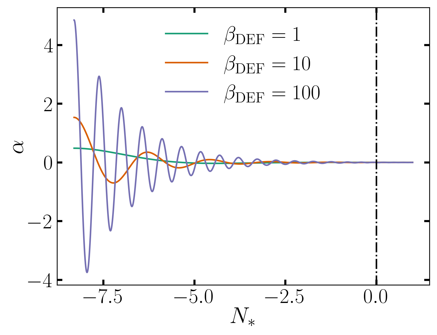
Figure 7: The evolution of the coupling $\alpha$ between matter and scalar field with different $\beta_{\mathrm{DEF}}$ in DEF theory. The initial conditions are $\phi^{\prime}=0$ and $\phi$ saturating the constraint of speed-up factor during nucleosynthesis [202]. The present coupling $\alpha_{0}=\alpha|_{N_{*}=0}$ is negligibly small.

Another interesting feature of the DEF theory is that when the gravitational field gets stronger, the compact star may scalarize spontaneously and become a scalarized star if the parameter $\beta_{\mathrm{DEF}}\lesssim-4$ [199, 34]. Spontaneous scalarization and general relativity attractor share different parameter spaces in the DEF theory and some generalized theories [198, 200, 203]. Adding another extra coupling between the scalar field and the Gauss-Bonnet term is a feasible solution to exhibit spontaneous scalarization in the strong-field regime and the spacetime behaves like general relativity at infinity as a cosmological attractor [204, 205].

In order to explain the accelerated expansion, the potential $V(\phi)$ cannot be zero. If one is interested in a scalar field with energy density of the same order as that of matter today, then the term $\rmd\ln V/\rmd\phi$ in Equation (3.35bbbrcc) turns out to be subdominant with respect to $(1-3w)\alpha$ during the radiation-domination epoch and most of the matter-domination epoch. At late times, the scalar potential term starts to dominate and the gravity is approximately described by general relativity as $\alpha\to 0$. By choosing the coupling function as

$$\alpha(\phi)=-Be^{-\beta\phi}$$ (3.35bbbrce)

and the Ratra-Peebles potential (3.28) for the scalar field, one obtains an approximate solution during the radiation and matter domination [206]

$$\phi(a_{*})\simeq\frac{1}{\beta}\ln\left[\beta B\ln\left(\frac{2}{3}+\frac{a_{*}}{a_{*}^{\mathrm{eq}}}\right)+C\right],$$ (3.35bbbrcf)

where $a_{*}^{\mathrm{eq}}$ is the value of the scale factor at the equivalence epoch (the cosmic time when $\rho_{\mathrm{r}}=\rho_{\mathrm{d}}$) and $C$ is a constant. This solution is an attractor in phase space and behaves as a subdominant contribution to the energy density that starts increasing during the matter-dominated era and eventually comes to dominate in the present era. The Doppler peaks are shifted toward higher multipoles and their height is changed with respect to minimally coupled models, providing a signature to look for in future CMB experiments [206].

4.4 Recapitulation and Possible Extension

A general action describing various couplings to the scalar field for different components of the Universe in the Einstein frame is given by

$$S[g^{*}_{\mu\nu},\phi,\Psi_{\mathrm{m}}^{(i)}]=\int\rmd^{4}x\sqrt{-g_{*}}\left[\frac{R_{*}}{2\kappa_{*}}-\frac{1}{2}g_{*}^{\mu\nu}\partial_{\mu}\phi\partial_{\nu}\phi-V(\phi)\right]+S_{\mathrm{m}}[g_{\mu\nu}^{(i)},\Psi_{\mathrm{m}}^{(i)}]$$ (3.35bbbrcg)

where $\Psi_{m}^{(i)}$ is the matter field coupled to the Jordan frame metric $g_{\mu\nu}^{(i)}$, related to the Einstein frame metric $g^{*}_{\mu\nu}$ via

$$g_{\mu\nu}^{(i)}=A^{2}_{i}(\phi)g^{*}_{\mu\nu}.$$ (3.35bbbrch)

The action (3.35bbbrcg) reduces to the general relativity if $A_{i}=1$, which means that each component of the Universe does not couple to the metric in the Einstein frame. In that case, metrics in the Jordan frame and the Einstein frame are the same. The quintessence model, in the framework of general relativity, relies on a self-interacting potential of the scalar field and a violation of the strong energy condition to provide necessary cosmic acceleration. During a slow-roll phase of the massive scalar field when its kinetic energy is much less than its self-interacting one, negative pressures are achieved, producing the desired cosmic acceleration. The potential, as the only degree of freedom in the quintessence model, can be quite sophisticated and has to be well shaped to reproduce the cosmic evolution or to exhibit interesting tracking properties. The coincidence problem is somehow moved to the specific choice of both an appropriate shape and energy scale for the self-interaction potential. Most of the potentials used in quintessence models come out of an effective theory of high-energy physics, leaving a glimpse into new physics. However, deriving such quintessence models (and also the k-essence extension models) from high-energy physics in a self-consistent framework is a challenging task, as combining all the cosmological, gravitational, and particle physics aspects raises many technical difficulties.

The quintessence scalar field minimally couples to gravitation and does not couple directly to ordinary matter. Hence, quintessence only modifies the background cosmic expansion and all the observations of gravity theory without the quintessence component remain the same. If matter fields couple to both scalar field and gravitation directly, the new “fifth” interaction yields a violation of the strong equivalence principle [207]. The non-minimal coupling changes physical coupling constants or inertial masses and as a consequence, modifies the way energies have been weighted in the cosmic history. In the case where the scalar field directly affects the couplings to the gravitational field and therefore makes the gravitational constant vary, one gets the scalar-tensor theories of gravity,

$$S[g^{*}_{\mu\nu},\phi,\Psi_{\mathrm{m}}]=\int\rmd^{4}x\sqrt{-g_{*}}\left[\frac{R_{*}}{2\kappa_{*}}-\frac{1}{2}g_{*}^{\mu\nu}\partial_{\mu}\phi\partial_{\nu}\phi-V(\phi)\right]+S_{\mathrm{m}}[A^{2}(\phi)g_{\mu\nu}^{*},\Psi_{\mathrm{m}}].$$ (3.35bbbrci)

If we consider that about 70% of the missing energy is the whole contribution of such a non-minimally coupled scalar field, it might be difficult to match the present tests of gravity without assuming the non-minimal couplings to be extremely weak. In fact, the coupled quintessence model corresponds to the case $A_{\mathrm{b}}=1$ for baryons while $A_{\rm dm}$ for dark matter varies with $\phi$, which reveals a non-universal coupling. This non-universal coupling solves the extremely small coupling problem, but the weak equivalent principle is severely violated. As for the chameleon cosmology, however, both baryons and dark matter are non-minimally coupled to the quintessence field as $A_{\mathrm{b}}=A_{\rm dm}=e^{\alpha\phi}$, with the mass of the scalar field being environmentally dependent. This offers the possibility of accounting for the present bounds of local tests of the strong and weak equivalent principles on the Earth and in the Solar system by the larger mass of the scalar field in a denser neighborhood than in the cosmological low-density limit. In order to do so, a specific self-interaction potential and a consequent violation of the strong energy condition have to be re-introduced. Another alternative model proposes that both $A_{\mathrm{b}}$ and $A_{\rm dm}$ depends on the scalar field, but not identical [208]. The self-interacting potential $V(\phi)$ is unnecessary in this model if two couplings are both assumed to be of order unity, and the cosmic acceleration is a generic prediction of the competition between different non-minimal couplings. Moreover, the attractor to which gravitation is driven depends on the ratio between the energy densities of ordinary matter and dark matter.

The most general 4-dimensional scalar-tensor theories having second-order equations of motion are the Horndeski theory [209, 210]

$$S_{\mathrm{H}}[g_{\mu\nu},\phi,\Psi_{\mathrm{m}}]=\sum_{i=2}^{5}\int\rmd^{4}x\sqrt{-g}\mathcal{L}_{i}+S_{\mathrm{m}}[g_{\mu\nu},\Psi_{\mathrm{m}}],$$ (3.35bbbrcj)

where the Lagrangian densities are

$$\mathcal{L}_{2}=G_{2}(\phi,X),$$ (3.35bbbrcka)

$$\mathcal{L}_{3}=G_{3}(\phi,X)\square\phi,$$ (3.35bbbrckb)

$$\mathcal{L}_{4}=G_{4}(\phi,X)R+G_{4X}\big{[}(\square\phi)^{2}-\nabla_{\mu}\nabla_{\nu}\phi\nabla^{\mu}\nabla^{\nu}\phi\big{]},$$ (3.35bbbrckc)

$$\mathcal{L}_{5}=G_{5}(\phi,X)G_{\mu\nu}\nabla^{\mu}\nabla^{\nu}\phi$$

$$-\frac{G_{5X}}{6}\Big{[}(\square\phi)^{3}-3\square\phi\nabla_{\mu}\nabla_{\nu}\phi\nabla^{\mu}\nabla^{\nu}\phi+2\nabla^{\mu}\nabla_{\alpha}\phi\nabla^{\alpha}\nabla_{\beta}\phi\nabla^{\beta}\nabla_{\mu}\phi\Big{]}.$$ (3.35bbbrckd)

The theory is termed as Horndeski theory because Kobayashi et al. [211] found that the action (3.35bbbrcj) is equivalent to the one discovered by Horndeski in 1974 [212]. Here, $G_{i}$ ($i=2,3,4,5$) are arbitrary functions of the scalar field $\phi$ and its kinetic energy $X$, while $G_{i\phi}$ and $G_{iX}$ represent the derivatives of functions $G_{i}$ with respect to $\phi$ and $X$, respectively. Due to the second-order property, there is no Ostrogradski instability [213] associated with the Hamiltonian unbounded from below.

In a flat FLRW background, the EOS parameter of the scalar field $\phi$ is

$$w_{\phi}=-1+\frac{2(q_{\mathrm{t}}-M_{\mathrm{Pl}}^{2})\dot{H}-D_{6}\ddot{\phi}+D_{7}\dot{\phi}}{\rho_{\phi}},$$ (3.35bbbrckcl)

where

$$q_{\mathrm{t}}=2G_{4}-2\dot{\phi}^{2}G_{4X}+\dot{\phi}^{2}G_{5\phi}-H\dot{\phi}^{3}G_{5X},$$ (3.35bbbrckcm)

and the definition of $D_{6,7}$ and energy density $\rho_{\phi}$ can be found in Ref. [214]. Since the evolution of $w_{\phi}$ is different depending on dark energy models, it is possible to distinguish them from observations, like SN Ia, CMB, BAO, LSSs, and weak lensing.

The propagation speed squared of the tensor perturbations in the Horndeski theories is [211]

$$c_{\mathrm{t}}^{2}=\frac{1}{q_{\mathrm{t}}}\Big{(}2G_{4}-\dot{\phi}^{2}G_{5\phi}-\dot{\phi}^{2}\ddot{\phi}G_{5X}\Big{)}.$$ (3.35bbbrckcn)

The detection of gravitational waves by GW170817 [215] from a binary neutron star merger together with the short gamma-ray burst GRB 170817A [216] constrained the propagation speed $c_{\mathrm{t}}$ of gravitational waves to be [217]

$$-3\times 10^{-15}<c_{\mathrm{t}}-1<7\times 10^{-16}.$$ (3.35bbbrckco)

If any fine tuning among functions is forbidden, one has $G_{4X}=G_{5\phi}=G_{5X}=0$, then the Horndeski theory is restricted to be of the form [218, 219, 220, 221]

$$S[g_{\mu\nu},\phi,\Psi_{\mathrm{m}}]=\int\rmd^{4}x\sqrt{-g}\big{[}G_{2}(\phi,X)+G_{3}(\phi,X)\square\phi+G_{4}(\phi)R\big{]}+S_{\mathrm{m}}[g_{\mu\nu},\Psi_{\mathrm{m}}].$$ (3.35bbbrckcp)

Each dark energy model or scalar-tensor gravity mentioned above corresponds to this reduced action (3.35bbbrckcp) with specific functions $G_{i}$ ($i=1,2,3$). The k-essence model (3.35ax) is given by the choice

$$G_{2}=P(\phi,X),\quad G_{3}=0,\quad G_{4}=\frac{M^{2}_{\mathrm{Pl}}}{2},$$ (3.35bbbrckcq)

and the extended quintessence model (3.35ac) is acquired if

$$G_{2}=\zeta(\phi)X-U(\phi),\quad G_{3}=0,\quad G_{4}=\frac{M^{2}_{\mathrm{Pl}}}{2}F(\phi).$$ (3.35bbbrckcr)

There are other modified gravity theories dubbed Galileon theories [209, 222, 210] containing scalar derivative self-interactions $G_{3}\neq 0$. In the original Galileon theory [209], the field equations of motion are invariant under the Galilean shift $\partial_{\mu}\phi\to\partial_{\mu}\phi+b_{\mu}$ in the Minkowski spacetime. In a curved spacetime, the Lagrangian of covariant Galileon theories [210] is constructed to keep the equations of motion up to the second order, while recovering the Galilean shift symmetry in the Minkowski limit. For covariant Galileons, there exist self-accelerating de Sitter attractors responsible for the late-time cosmic acceleration [223, 224, 225]. However, the covariant Galileons with quartic and quintic Lagrangians do not pass the test of tensor perturbation without fine-tuning parameters.

The generally considered function of $G_{3}$ is the form of cubic Galileon $X\square\phi$, which arises in the Dvali-Gabadadze-Porrati braneworld model due to the mixture between longitudinal and transverse gravitons [226] and also in the Dirac-Born-Infeld decoupling theory with bulk Lovelock invariants [227]. This derivative self-interaction can suppress the propagation of fifth forces in local regions of the Universe with the Vainshtein mechanism [228], while modifying the gravitational interaction at cosmological distances [229, 230, 231, 232].

There are two kinds of solutions that displace the present cosmic acceleration in minimally coupled cubic Galileon theories ($G_{4}=M_{\mathrm{Pl}}^{2}/2$). One is the solution with a constant $X$ in the absence of potential [224, 225], but it is in tension with the observational data of redshift-space distortions, weak lensing, and integrated Sachs-Wolfe-galaxy cross-correlations [233]. The other is the solution in cubic Galileon with a linear potential $V\propto\phi$ or other specific form [234], and it is the potential that drives the late-time accelerated expansion [222]. In recent years, the Galileon ghost condensate with $G_{2}=X+c_{2}X^{2}$ has received more attention for alleviating the problem of tracker solutions found in other cubic Galileon theories and improving the compatibility with the Planck CMB data [235]. Furthermore, the cosmology of non-minimally coupled cubic Galileons has also been studied [236, 225], including constraints on the coupling from Solar system and binary pulsar tests [237, 238, 239, 240].

It is conceivable that the evolution of the Universe within Horndeski theory undergoes a diverse and dynamic process. Various phenomena such as late-time tracking, scaling, quintessence, and phantom behaviors are within the realm of possibility, which offer promising avenues for addressing the fine-tuning and coincidence problems. However, the intricate equations of motion arising from these model prevent simple applications of dynamical systems theories and extremely complicated analysis are required, often dealing with non-compact high-dimensional autonomous systems.

5 A Brief Outlook

We have presented a concise overview of two distinct physical mechanisms—dark energy and modified gravity—to elucidate the accelerated expansion of the Universe. The technique of dynamical system is applied to typical models—quintessence, coupled quintessence, and extended quintessence—to qualitatively describe the evolution of the Universe and the emergence of an accelerated expansion stage. The primary focus of the discussion revolves around constant couplings and exponential potentials, while more specific and sophisticated models are left to be explored in the original literature.

By assuming that the vacuum energy is either negligible or does not contribute to the gravitational field equation, modern study of cosmological constant problem on the classical level inquiries into identifying mechanisms responsible for the current acceleration of the Universe, so as to avoid the original fine-tuning problem in $\Lambda$CDM model. Nevertheless, for theories like quintessence to accurately portray the present state of the Universe, characterized by roughly equal proportions of matter and dark energy, the initial conditions of the Universe often need to be finely tuned to an extremely narrow range, thus presenting another instance of fine-tuning. A solution to the so-called coincidence problem would be to establish that the state where $\Omega_{\mathrm{m}}\simeq 0.3$ and $\Omega_{\mathrm{de}}\simeq 0.7$ is indeed the ultimate fate of the Universe, such as the coupled quintessence model. Two additional strategies that potentially alleviate the coincidence problem include expanding the range of initial conditions to accommodate existing observations of the Universe’s evolution and permitting the Universe to evolve at a gradual pace towards a state vastly different from its current configuration, with tracking solutions and some interacting dark energy model being corresponding examples. Unlike the other two issues, the Hubble tension and more tensions observed in cosmological observations represent genuine problems that demand resolution but continue to harbor uncertainty. The interacting dark energy and chameleon dark energy discussed in this review have opportunity to solve these tensions. While these tensions are receiving increased attention, the scope of this review does not delve deeply into the early Universe, and more information can be found in comprehensive review papers such as Refs. [241, 242, 243].

At present, dark energy models are not particularly favored over the $\Lambda$CDM model from the current observational data, though they are better equipped to deal with various challenges. Furthermore, there is no concrete observational signature for non-minimally coupled theories, despite that they usually have much richer properties in dynamics. In the coming decades, LSS and CMB surveys will possess the capability to probe dynamical dark energy and deviations from general relativity with greater precision [244, 245, 246, 247]. Additionally, new methods of observing cosmology like gamma-ray burst detection [248, 249] and gravitational-wave observation [250, 251] will contribute to the discourse. These advancements hopefully will either rule out some dark energy and modified gravity models or yield a breakthrough in cosmology and physics by confirming new fundamental ingredients.

Numerous models exist to elucidate the current accelerated expansion of the Universe through the employment of scalar fields; however, we are unable to discuss all of them due to the limitation of space. Certainly, there are models that explain the expansion in terms of fluids or other fields beyond scalar fields, while some specific theoretical models also propose alternatives to the solutions discussed in this review [252]. We encourage the audience to explore additional reviews and specialized literature for supplementary insights, both within and beyond the reference of this review. The references we quote absolutely do not represent all the research in the field, and we regret any oversight of significant literature.

References

References

- [1] Riess A G et al (Supernova Search Team) 1998 Observational evidence from supernovae for an accelerating universe and a cosmological constant Astron. J. 116 1009–1038 (Preprint arXiv:astro-ph/9805201)
- [2] Perlmutter S et al (Supernova Cosmology Project) 1999 Measurements of and from 42 high redshift supernovae Astrophys. J. 517 565–586 (Preprint arXiv:astro-ph/9812133)
- [3] Podariu S and Ratra B 2000 Supernovae Ia constraints on a time variable cosmological ’constant’ Astrophys. J. 532 109–117 (Preprint arXiv:astro-ph/9910527)
- [4] Riess A G et al 2007 New Hubble Space Telescope Discoveries of Type Ia Supernovae at z=1: Narrowing Constraints on the Early Behavior of Dark Energy Astrophys. J. 659 98–121 (Preprint arXiv:astro-ph/0611572)
- [5] Spergel D N et al (WMAP) 2003 First year Wilkinson Microwave Anisotropy Probe (WMAP) observations: Determination of cosmological parameters Astrophys. J. Suppl. 148 175–194 (Preprint arXiv:astro-ph/0302209)
- [6] Hinshaw G et al (WMAP) 2009 Five-Year Wilkinson Microwave Anisotropy Probe (WMAP) Observations: Data Processing, Sky Maps, and Basic Results Astrophys. J. Suppl. 180 225–245 (Preprint arXiv:0803.0732)
- [7] Komatsu E et al (WMAP) 2009 Five-Year Wilkinson Microwave Anisotropy Probe (WMAP) Observations: Cosmological Interpretation Astrophys. J. Suppl. 180 330–376 (Preprint arXiv:0803.0547)
- [8] Komatsu E et al (WMAP) 2011 Seven-Year Wilkinson Microwave Anisotropy Probe (WMAP) Observations: Cosmological Interpretation Astrophys. J. Suppl. 192 18 (Preprint arXiv:1001.4538)
- [9] Ade P A R et al (Planck) 2014 Planck 2013 results. XVI. Cosmological parameters Astron. Astrophys. 571 A16 (Preprint arXiv:1303.5076)
- [10] Ade P A R et al (Planck) 2016 Planck 2015 results. XIII. Cosmological parameters Astron. Astrophys. 594 A13 (Preprint arXiv:1502.01589)
- [11] Aghanim N et al (Planck) 2020 Planck 2018 results. VI. Cosmological parameters Astron. Astrophys. 641 A6 [Erratum: Astron.Astrophys. 652, C4 (2021)] (Preprint arXiv:1807.06209)
- [12] Eisenstein D J et al (SDSS) 2005 Detection of the Baryon Acoustic Peak in the Large-Scale Correlation Function of SDSS Luminous Red Galaxies Astrophys. J. 633 560–574 (Preprint arXiv:astro-ph/0501171)
- [13] Blake C et al 2011 The WiggleZ Dark Energy Survey: mapping the distance-redshift relation with baryon acoustic oscillations Mon. Not. Roy. Astron. Soc. 418 1707–1724 (Preprint arXiv:1108.2635)
- [14] Beutler F, Blake C, Colless M, Jones D H, Staveley-Smith L, Campbell L, Parker Q, Saunders W and Watson F 2011 The 6dF Galaxy Survey: Baryon Acoustic Oscillations and the Local Hubble Constant Mon. Not. Roy. Astron. Soc. 416 3017–3032 (Preprint arXiv:1106.3366)
- [15] Anderson L et al (BOSS) 2014 The clustering of galaxies in the SDSS-III Baryon Oscillation Spectroscopic Survey: baryon acoustic oscillations in the Data Releases 10 and 11 Galaxy samples Mon. Not. Roy. Astron. Soc. 441 24–62 (Preprint arXiv:1312.4877)
- [16] Ross A J, Samushia L, Howlett C, Percival W J, Burden A and Manera M 2015 The clustering of the SDSS DR7 main Galaxy sample – I. A 4 per cent distance measure at Mon. Not. Roy. Astron. Soc. 449 835–847 (Preprint arXiv:1409.3242)
- [17] Alam S et al (BOSS) 2017 The clustering of galaxies in the completed SDSS-III Baryon Oscillation Spectroscopic Survey: cosmological analysis of the DR12 galaxy sample Mon. Not. Roy. Astron. Soc. 470 2617–2652 (Preprint arXiv:1607.03155)
- [18] Ata M et al 2018 The clustering of the SDSS-IV extended Baryon Oscillation Spectroscopic Survey DR14 quasar sample: first measurement of baryon acoustic oscillations between redshift 0.8 and 2.2 Mon. Not. Roy. Astron. Soc. 473 4773–4794 (Preprint arXiv:1705.06373)
- [19] Allen S W, Schmidt R W, Ebeling H, Fabian A C and van Speybroeck L 2004 Constraints on dark energy from Chandra observations of the largest relaxed galaxy clusters Mon. Not. Roy. Astron. Soc. 353 457 (Preprint arXiv:astro-ph/0405340)
- [20] Chen G and Ratra B 2004 Constraints on scalar-field dark energy from galaxy cluster gas mass fraction versus redshift Astrophys. J. Lett. 612 L1–4 (Preprint arXiv:astro-ph/0405636)
- [21] Tegmark M et al (SDSS) 2004 Cosmological parameters from SDSS and WMAP Phys. Rev. D 69 103501 (Preprint arXiv:astro-ph/0310723)
- [22] Seljak U et al (SDSS) 2005 Cosmological parameter analysis including SDSS Ly-alpha forest and galaxy bias: Constraints on the primordial spectrum of fluctuations, neutrino mass, and dark energy Phys. Rev. D 71 103515 (Preprint arXiv:astro-ph/0407372)
- [23] Percival W J, Cole S, Eisenstein D J, Nichol R C, Peacock J A, Pope A C and Szalay A S 2007 Measuring the Baryon Acoustic Oscillation scale using the SDSS and 2dFGRS Mon. Not. Roy. Astron. Soc. 381 1053–1066 (Preprint arXiv:0705.3323)
- [24] Kwan J et al (DES) 2017 Cosmology from large-scale galaxy clustering and galaxy–galaxy lensing with Dark Energy Survey Science Verification data Mon. Not. Roy. Astron. Soc. 464 4045–4062 (Preprint arXiv:1604.07871)
- [25] Will C M 2014 The Confrontation between General Relativity and Experiment Living Rev. Rel. 17 4 (Preprint arXiv:1403.7377)
- [26] Padmanabhan T 2003 Cosmological constant: The Weight of the vacuum Phys. Rept. 380 235–320 (Preprint arXiv:hep-th/0212290)
- [27] Copeland E J, Sami M and Tsujikawa S 2006 Dynamics of dark energy Int. J. Mod. Phys. D 15 1753–1936 (Preprint arXiv:hep-th/0603057)
- [28] Damour T and Esposito-Farese G 1992 Tensor multiscalar theories of gravitation Class. Quant. Grav. 9 2093–2176
- [29] Faraoni V 2004 Cosmology in scalar tensor gravity ISBN 978-1-4020-1988-3
- [30] Fujii Y and Maeda K 2007 The scalar-tensor theory of gravitation Cambridge Monographs on Mathematical Physics (Cambridge University Press) ISBN 978-0-521-03752-5, 978-0-521-81159-0, 978-0-511-02988-2
- [31] Quiros I 2019 Selected topics in scalar–tensor theories and beyond Int. J. Mod. Phys. D 28 1930012 (Preprint arXiv:1901.08690)
- [32] Barausse E et al 2020 Prospects for Fundamental Physics with LISA Gen. Rel. Grav. 52 81 (Preprint arXiv:2001.09793)
- [33] Arun K G et al (LISA) 2022 New horizons for fundamental physics with LISA Living Rev. Rel. 25 4 (Preprint arXiv:2205.01597)
- [34] Doneva D D, Ramazanoğlu F M, Silva H O, Sotiriou T P and Yazadjiev S S 2022 Scalarization (Preprint arXiv:2211.01766)
- [35] Shao L and Wex N 2016 Tests of gravitational symmetries with radio pulsars Sci. China Phys. Mech. Astron. 59 699501 (Preprint arXiv:1604.03662)
- [36] Shao L, Sennett N, Buonanno A, Kramer M and Wex N 2017 Constraining nonperturbative strong-field effects in scalar-tensor gravity by combining pulsar timing and laser-interferometer gravitational-wave detectors Phys. Rev. X 7 041025 (Preprint arXiv:1704.07561)
- [37] Clifton T, Ferreira P G, Padilla A and Skordis C 2012 Modified Gravity and Cosmology Phys. Rept. 513 1–189 (Preprint arXiv:1106.2476)
- [38] Peebles P J E and Ratra B 2003 The Cosmological Constant and Dark Energy Rev. Mod. Phys. 75 559–606 (Preprint arXiv:astro-ph/0207347)
- [39] Avsajanishvili O, Chitov G Y, Kahniashvili T, Mandal S and Samushia L 2024 Observational Constraints on Dynamical Dark Energy Models Universe 10 122 (Preprint arXiv:2310.16911)
- [40] Einstein A 1917 Cosmological Considerations in the General Theory of Relativity Sitzungsber. Preuss. Akad. Wiss. Berlin (Math. Phys. ) 1917 142–152
- [41] Eddington A S 1930 On the Instability of Einstein’s Spherical World Mon. Not. Roy. Astron. Soc. 90 668–678
- [42] Hubble E 1929 A relation between distance and radial velocity among extra-galactic nebulae Proc. Nat. Acad. Sci. 15 168–173
- [43] Sandage A 1961 The Ability of the 200-Inch Telescope to Discriminate Between Selected World Models Astrophys. J. 133 355–392
- [44] Petrosian V, Salpeter E and Szekeres P 1967 Quasi-Stellar Objects in Universes with Non-Zero Cosmological Constant Astrophys. J. 147 1222
- [45] Turner M S, Steigman G and Krauss L M 1984 The Flatness of the Universe: Reconciling Theoretical Prejudices with Observational Data Phys. Rev. Lett. 52 2090–2093
- [46] Peebles P J E 1984 Tests of Cosmological Models Constrained by Inflation Astrophys. J. 284 439–444
- [47] Weinberg S 1989 The Cosmological Constant Problem Rev. Mod. Phys. 61 1–23
- [48] Carroll S M, Press W H and Turner E L 1992 The Cosmological constant Ann. Rev. Astron. Astrophys. 30 499–542
- [49] Zel’dovich Y B, Krasinski A and Zeldovich Y B 1968 The Cosmological constant and the theory of elementary particles Sov. Phys. Usp. 11 381–393
- [50] Rugh S E and Zinkernagel H 2002 The Quantum vacuum and the cosmological constant problem Stud. Hist. Phil. Sci. B 33 663–705 (Preprint arXiv:hep-th/0012253)
- [51] Martin J 2012 Everything You Always Wanted To Know About The Cosmological Constant Problem (But Were Afraid To Ask) Comptes Rendus Physique 13 566–665 (Preprint arXiv:1205.3365)
- [52] Burgess C P 2015 The Cosmological Constant Problem: Why it’s hard to get Dark Energy from Micro-physics 100e Ecole d’Ete de Physique: Post-Planck Cosmology pp 149–197 (Preprint arXiv:1309.4133)
- [53] Weinberg S 1996 Theories of the cosmological constant Conference on Critical Dialogs in Cosmology pp 195–203 (Preprint arXiv:astro-ph/9610044)
- [54] Green M B, Schwarz J H and Witten E 1988 SUPERSTRING THEORY. VOL. 1: INTRODUCTION Cambridge Monographs on Mathematical Physics ISBN 978-0-521-35752-4
- [55] Rovelli C 2004 Quantum gravity Cambridge Monographs on Mathematical Physics (Cambridge, UK: Univ. Pr.)
- [56] Rovelli C and Vidotto F 2014 Covariant Loop Quantum Gravity: An Elementary Introduction to Quantum Gravity and Spinfoam Theory Cambridge Monographs on Mathematical Physics (Cambridge University Press) ISBN 978-1-107-06962-6, 978-1-316-14729-0
- [57] Wess J and Bagger J 1992 Supersymmetry and supergravity (Princeton, NJ, USA: Princeton University Press) ISBN 978-0-691-02530-8
- [58] Schwinger J S 1967 Sources and electrodynamics Phys. Rev. 158 1391–1407
- [59] Schwinger J S 1968 Sources and gravitons Phys. Rev. 173 1264–1272
- [60] Schwinger J S 1968 Sources and magnetic charge Phys. Rev. 173 1536–1544
- [61] Akrami Y et al (CANTATA) 2021 Modified Gravity and Cosmology: An Update by the CANTATA Network (Springer) ISBN 978-3-030-83714-3, 978-3-030-83717-4, 978-3-030-83715-0 (Preprint arXiv:2105.12582)
- [62] Huterer D and Turner M S 1999 Prospects for probing the dark energy via supernova distance measurements Phys. Rev. D 60 081301 (Preprint arXiv:astro-ph/9808133)
- [63] Perlmutter S, Turner M S and White M J 1999 Constraining dark energy with SNe Ia and large scale structure Phys. Rev. Lett. 83 670–673 (Preprint arXiv:astro-ph/9901052)
- [64] Verde L, Treu T and Riess A G 2019 Tensions between the Early and the Late Universe Nature Astron. 3 891 (Preprint arXiv:1907.10625)
- [65] Riess A G, Anand G S, Yuan W, Casertano S, Dolphin A, Macri L M, Breuval L, Scolnic D, Perrin M and Anderson I R 2024 JWST Observations Reject Unrecognized Crowding of Cepheid Photometry as an Explanation for the Hubble Tension at 8 Confidence Astrophys. J. Lett. 962 L17 (Preprint arXiv:2401.04773)
- [66] Guth A H 1981 The Inflationary Universe: A Possible Solution to the Horizon and Flatness Problems Phys. Rev. D 23 347–356
- [67] Linde A D 1982 A New Inflationary Universe Scenario: A Possible Solution of the Horizon, Flatness, Homogeneity, Isotropy and Primordial Monopole Problems Phys. Lett. B 108 389–393
- [68] Caldwell R R, Dave R and Steinhardt P J 1998 Cosmological imprint of an energy component with general equation of state Phys. Rev. Lett. 80 1582–1585 (Preprint arXiv:astro-ph/9708069)
- [69] Ratra B and Peebles P J E 1988 Cosmological Consequences of a Rolling Homogeneous Scalar Field Phys. Rev. D 37 3406
- [70] Wetterich C 1988 Cosmology and the Fate of Dilatation Symmetry Nucl. Phys. B 302 668–696 (Preprint arXiv:1711.03844)
- [71] Caldwell R R and Linder E V 2005 The Limits of quintessence Phys. Rev. Lett. 95 141301 (Preprint arXiv:astro-ph/0505494)
- [72] Frieman J A, Hill C T, Stebbins A and Waga I 1995 Cosmology with ultralight pseudo Nambu-Goldstone bosons Phys. Rev. Lett. 75 2077–2080 (Preprint arXiv:astro-ph/9505060)
- [73] Chiba T, De Felice A and Tsujikawa S 2013 Observational constraints on quintessence: thawing, tracker, and scaling models Phys. Rev. D 87 083505 (Preprint arXiv:1210.3859)
- [74] Zlatev I, Wang L M and Steinhardt P J 1999 Quintessence, cosmic coincidence, and the cosmological constant Phys. Rev. Lett. 82 896–899 (Preprint arXiv:astro-ph/9807002)
- [75] Chiba T 2010 The Equation of State of Tracker Fields Phys. Rev. D 81 023515 (Preprint arXiv:0909.4365)
- [76] Durrive J B, Ooba J, Ichiki K and Sugiyama N 2018 Updated observational constraints on quintessence dark energy models Phys. Rev. D 97 043503 (Preprint arXiv:1801.09446)
- [77] Coley A A 2003 Dynamical systems and cosmology (Dordrecht, Netherlands: Kluwer)
- [78] Bahamonde S, Böhmer C G, Carloni S, Copeland E J, Fang W and Tamanini N 2018 Dynamical systems applied to cosmology: dark energy and modified gravity Phys. Rept. 775-777 1–122 (Preprint arXiv:1712.03107)
- [79] Copeland E J, Liddle A R and Wands D 1998 Exponential potentials and cosmological scaling solutions Phys. Rev. D 57 4686–4690 (Preprint arXiv:gr-qc/9711068)
- [80] Tsujikawa S 2010 Dark energy: investigation and modeling (Preprint arXiv:1004.1493)
- [81] Wainwright J and Ellis G F R 2005 Dynamical Systems in Cosmology
- [82] Ferreira P G and Joyce M 1998 Cosmology with a primordial scaling field Phys. Rev. D 58 023503 (Preprint arXiv:astro-ph/9711102)
- [83] Barreiro T, Copeland E J and Nunes N J 2000 Quintessence arising from exponential potentials Phys. Rev. D 61 127301 (Preprint arXiv:astro-ph/9910214)
- [84] Sahni V and Wang L M 2000 A New cosmological model of quintessence and dark matter Phys. Rev. D 62 103517 (Preprint arXiv:astro-ph/9910097)
- [85] Albrecht A and Skordis C 2000 Phenomenology of a realistic accelerating universe using only Planck scale physics Phys. Rev. Lett. 84 2076–2079 (Preprint arXiv:astro-ph/9908085)
- [86] Dodelson S, Kaplinghat M and Stewart E 2000 Solving the Coincidence Problem : Tracking Oscillating Energy Phys. Rev. Lett. 85 5276–5279 (Preprint arXiv:astro-ph/0002360)
- [87] Amendola L and Tsujikawa S 2010 Dark energy: theory and observations (Cambridge University Press)
- [88] de la Macorra A and Piccinelli G 2000 General scalar fields as quintessence Phys. Rev. D 61 123503 (Preprint arXiv:hep-ph/9909459)
- [89] Ng S C C, Nunes N J and Rosati F 2001 Applications of scalar attractor solutions to cosmology Phys. Rev. D 64 083510 (Preprint arXiv:astro-ph/0107321)
- [90] Steinhardt P J, Wang L M and Zlatev I 1999 Cosmological tracking solutions Phys. Rev. D 59 123504 (Preprint arXiv:astro-ph/9812313)
- [91] Tsujikawa S 2013 Quintessence: A Review Class. Quant. Grav. 30 214003 (Preprint arXiv:1304.1961)
- [92] Ma C P and Bertschinger E 1995 Cosmological perturbation theory in the synchronous and conformal Newtonian gauges Astrophys. J. 455 7–25 (Preprint arXiv:astro-ph/9506072)
- [93] Corasaniti P S, Kunz M, Parkinson D, Copeland E J and Bassett B A 2004 The Foundations of observing dark energy dynamics with the Wilkinson Microwave Anisotropy Probe Phys. Rev. D 70 083006 (Preprint arXiv:astro-ph/0406608)
- [94] Alam U, Sahni V, Saini T D and Starobinsky A A 2004 Is there supernova evidence for dark energy metamorphosis ? Mon. Not. Roy. Astron. Soc. 354 275 (Preprint arXiv:astro-ph/0311364)
- [95] Zhao G B, Xia J Q, Feng B and Zhang X 2007 Probing dynamics of dark energy with supernova, galaxy clustering and the three-year wilkinson microwave anisotropy probe (wmap) observations Int. J. Mod. Phys. D 16 1229–1242 (Preprint arXiv:astro-ph/0603621)
- [96] Caldwell R R 2002 A Phantom menace? Phys. Lett. B 545 23–29 (Preprint arXiv:astro-ph/9908168)
- [97] Caldwell R R, Kamionkowski M and Weinberg N N 2003 Phantom energy and cosmic doomsday Phys. Rev. Lett. 91 071301 (Preprint arXiv:astro-ph/0302506)
- [98] Ellis G F R, Maartens R and MacCallum M A H 2012 Relativistic Cosmology (Cambridge University Press)
- [99] Carroll S M, Hoffman M and Trodden M 2003 Can the dark energy equation-of-state parameter be less than ? Phys. Rev. D 68 023509 (Preprint arXiv:astro-ph/0301273)
- [100] Singh P, Sami M and Dadhich N 2003 Cosmological dynamics of phantom field Phys. Rev. D 68 023522 (Preprint arXiv:hep-th/0305110)
- [101] Cline J M, Jeon S and Moore G D 2004 The Phantom menaced: Constraints on low-energy effective ghosts Phys. Rev. D 70 043543 (Preprint arXiv:hep-ph/0311312)
- [102] Urena-Lopez L A 2005 Scalar phantom energy as a cosmological dynamical system JCAP 09 013 (Preprint arXiv:astro-ph/0507350)
- [103] Elizalde E, Nojiri S and Odintsov S D 2004 Late-time cosmology in (phantom) scalar-tensor theory: Dark energy and the cosmic speed-up Phys. Rev. D 70 043539 (Preprint arXiv:hep-th/0405034)
- [104] Xia J Q, Cai Y F, Qiu T T, Zhao G B and Zhang X 2008 Constraints on the Sound Speed of Dynamical Dark Energy Int. J. Mod. Phys. D 17 1229–1243 (Preprint arXiv:astro-ph/0703202)
- [105] Feng B, Wang X L and Zhang X M 2005 Dark energy constraints from the cosmic age and supernova Phys. Lett. B 607 35–41 (Preprint arXiv:astro-ph/0404224)
- [106] Guo Z K, Piao Y S, Zhang X M and Zhang Y Z 2005 Cosmological evolution of a quintom model of dark energy Phys. Lett. B 608 177–182 (Preprint arXiv:astro-ph/0410654)
- [107] Leon G, Leyva Y and Socorro J 2014 Quintom phase-space: beyond the exponential potential Phys. Lett. B 732 285–297 (Preprint arXiv:1208.0061)
- [108] Cai Y F, Saridakis E N, Setare M R and Xia J Q 2010 Quintom Cosmology: Theoretical implications and observations Phys. Rept. 493 1–60 (Preprint arXiv:0909.2776)
- [109] Saridakis E N and Weller J M 2010 A Quintom scenario with mixed kinetic terms Phys. Rev. D 81 123523 (Preprint arXiv:0912.5304)
- [110] Wei H, Cai R G and Zeng D F 2005 Hessence: A New view of quintom dark energy Class. Quant. Grav. 22 3189–3202 (Preprint arXiv:hep-th/0501160)
- [111] Wei H and Cai R G 2005 Cosmological evolution of hessence dark energy and avoidance of big rip Phys. Rev. D 72 123507 (Preprint arXiv:astro-ph/0509328)
- [112] Alimohammadi M and Mohseni Sadjadi H 2006 Attractor solutions for general hessence dark energy Phys. Rev. D 73 083527 (Preprint arXiv:hep-th/0602268)
- [113] Armendariz-Picon C, Damour T and Mukhanov V F 1999 k - inflation Phys. Lett. B 458 209–218 (Preprint arXiv:hep-th/9904075)
- [114] Gasperini M and Veneziano G 2003 The Pre - big bang scenario in string cosmology Phys. Rept. 373 1–212 (Preprint arXiv:hep-th/0207130)
- [115] Arkani-Hamed N, Cheng H C, Luty M A and Mukohyama S 2004 Ghost condensation and a consistent infrared modification of gravity JHEP 05 074 (Preprint arXiv:hep-th/0312099)
- [116] Garousi M R 2000 Tachyon couplings on nonBPS D-branes and Dirac-Born-Infeld action Nucl. Phys. B 584 284–299 (Preprint arXiv:hep-th/0003122)
- [117] Sen A 2002 Rolling tachyon JHEP 04 048 (Preprint arXiv:hep-th/0203211)
- [118] Silverstein E and Tong D 2004 Scalar speed limits and cosmology: Acceleration from D-cceleration Phys. Rev. D 70 103505 (Preprint arXiv:hep-th/0310221)
- [119] Alishahiha M, Silverstein E and Tong D 2004 DBI in the sky Phys. Rev. D 70 123505 (Preprint arXiv:hep-th/0404084)
- [120] Chiba T, Okabe T and Yamaguchi M 2000 Kinetically driven quintessence Phys. Rev. D 62 023511 (Preprint arXiv:astro-ph/9912463)
- [121] Malquarti M, Copeland E J, Liddle A R and Trodden M 2003 A New view of k-essence Phys. Rev. D 67 123503 (Preprint arXiv:astro-ph/0302279)
- [122] Garriga J and Mukhanov V F 1999 Perturbations in k-inflation Phys. Lett. B 458 219–225 (Preprint arXiv:hep-th/9904176)
- [123] Piazza F and Tsujikawa S 2004 Dilatonic ghost condensate as dark energy JCAP 07 004 (Preprint arXiv:hep-th/0405054)
- [124] Babichev E, Mukhanov V and Vikman A 2008 k-Essence, superluminal propagation, causality and emergent geometry JHEP 02 101 (Preprint arXiv:0708.0561)
- [125] Tsujikawa S 2006 General analytic formulae for attractor solutions of scalar-field dark energy models and their multi-field generalizations Phys. Rev. D 73 103504 (Preprint arXiv:hep-th/0601178)
- [126] Amendola L, Quartin M, Tsujikawa S and Waga I 2006 Challenges for scaling cosmologies Phys. Rev. D 74 023525 (Preprint arXiv:astro-ph/0605488)
- [127] Armendariz-Picon C, Mukhanov V F and Steinhardt P J 2000 A Dynamical solution to the problem of a small cosmological constant and late time cosmic acceleration Phys. Rev. Lett. 85 4438–4441 (Preprint arXiv:astro-ph/0004134)
- [128] Armendariz-Picon C, Mukhanov V F and Steinhardt P J 2001 Essentials of k essence Phys. Rev. D 63 103510 (Preprint arXiv:astro-ph/0006373)
- [129] Bonvin C, Caprini C and Durrer R 2006 A no-go theorem for k-essence dark energy Phys. Rev. Lett. 97 081303 (Preprint arXiv:astro-ph/0606584)
- [130] De-Santiago J, Cervantes-Cota J L and Wands D 2013 Cosmological phase space analysis of the F(X) - V() scalar field and bouncing solutions Phys. Rev. D 87 023502 (Preprint arXiv:1204.3631)
- [131] Bento M C, Bertolami O and Sen A A 2002 Generalized Chaplygin gas, accelerated expansion and dark energy matter unification Phys. Rev. D 66 043507 (Preprint arXiv:gr-qc/0202064)
- [132] Scherrer R J 2004 Purely kinetic k-essence as unified dark matter Phys. Rev. Lett. 93 011301 (Preprint arXiv:astro-ph/0402316)
- [133] Bertacca D, Matarrese S and Pietroni M 2007 Unified Dark Matter in Scalar Field Cosmologies Mod. Phys. Lett. A 22 2893–2907 (Preprint arXiv:astro-ph/0703259)
- [134] Fukuyama T, Morikawa M and Tatekawa T 2008 Cosmic structures via Bose Einstein condensation and its collapse JCAP 06 033 (Preprint arXiv:0705.3091)
- [135] Olive K A et al (Particle Data Group) 2014 Review of Particle Physics Chin. Phys. C 38 090001
- [136] Wang B, Abdalla E, Atrio-Barandela F and Pavon D 2016 Dark Matter and Dark Energy Interactions: Theoretical Challenges, Cosmological Implications and Observational Signatures Rept. Prog. Phys. 79 096901 (Preprint arXiv:1603.08299)
- [137] Wang B, Abdalla E, Atrio-Barandela F and Pavón D 2024 Further understanding the interaction between dark energy and dark matter: current status and future directions Rept. Prog. Phys. 87 036901 (Preprint arXiv:2402.00819)
- [138] Zimdahl W and Pavon D 2001 Interacting quintessence Phys. Lett. B 521 133–138 (Preprint arXiv:astro-ph/0105479)
- [139] Chimento L P, Jakubi A S, Pavon D and Zimdahl W 2003 Interacting quintessence solution to the coincidence problem Phys. Rev. D 67 083513 (Preprint arXiv:astro-ph/0303145)
- [140] del Campo S, Herrera R, Olivares G and Pavon D 2006 Interacting models of soft coincidence Phys. Rev. D 74 023501 (Preprint arXiv:astro-ph/0606520)
- [141] De Felice A and Tsujikawa S 2010 f(R) theories Living Rev. Rel. 13 3 (Preprint arXiv:1002.4928)
- [142] He J H, Wang B and Abdalla E 2011 Deep connection between f(R) gravity and the interacting dark sector model Phys. Rev. D 84 123526 (Preprint arXiv:1109.1730)
- [143] Shahalam M, Pathak S D, Li S, Myrzakulov R and Wang A 2017 Dynamics of coupled phantom and tachyon fields Eur. Phys. J. C 77 686 (Preprint arXiv:1702.04720)
- [144] Gumjudpai B, Naskar T, Sami M and Tsujikawa S 2005 Coupled dark energy: Towards a general description of the dynamics JCAP 06 007 (Preprint arXiv:hep-th/0502191)
- [145] Farajollahi H and Salehi A 2011 A New approach in stability analysis: case study: tachyon cosmology with non-minimally coupled scalar field-matter Phys. Rev. D 83 124042 (Preprint arXiv:1106.0091)
- [146] Farajollahi H, Salehi A, Tayebi F and Ravanpak A 2011 Stability Analysis in Tachyonic Potential Chameleon cosmology JCAP 05 017 (Preprint arXiv:1105.4045)
- [147] Mahata N and Chakraborty S 2015 Dynamical system analysis for DBI dark energy interacting with dark matter Mod. Phys. Lett. A 30 1550009 (Preprint arXiv:1501.04441)
- [148] Kaeonikhom C, Singleton D, Sushkov S V and Yongram N 2012 Dynamics of Dirac-Born-Infeld dark energy interacting with dark matter Phys. Rev. D 86 124049 (Preprint arXiv:1209.5219)
- [149] Jordan P 1955 Schwerkraft und weltall: Grundlagen der theoretischen kosmologie Die Wissenschaft
- [150] Brans C and Dicke R H 1961 Mach’s principle and a relativistic theory of gravitation Phys. Rev. 124 925–935
- [151] Bergmann P G 1968 Comments on the scalar tensor theory Int. J. Theor. Phys. 1 25–36
- [152] Wagoner R V 1970 Scalar tensor theory and gravitational waves Phys. Rev. D 1 3209–3216
- [153] Damour T 2009 Binary Systems as Test-beds of Gravity Theories Physics of Relativistic Objects in Compact Binaries: From Birth to Coalescence vol 359 ed Colpi M, Casella P, Gorini V, Moschella U and Possenti A (Springer, Dordrecht) p 1 (Preprint arXiv:0704.0749)
- [154] Wetterich C 1995 The Cosmon model for an asymptotically vanishing time dependent cosmological ’constant’ Astron. Astrophys. 301 321–328 (Preprint arXiv:hep-th/9408025)
- [155] Amendola L 2000 Coupled quintessence Phys. Rev. D 62 043511 (Preprint arXiv:astro-ph/9908023)
- [156] Damour T, Gibbons G W and Gundlach C 1990 Dark Matter, Time Varying , and a Dilaton Field Phys. Rev. Lett. 64 123–126
- [157] Casas J A, Garcia-Bellido J and Quiros M 1992 Scalar - tensor theories of gravity with phi dependent masses Class. Quant. Grav. 9 1371–1384 (Preprint arXiv:hep-ph/9204213)
- [158] Holden D J and Wands D 2000 Selfsimilar cosmological solutions with a nonminimally coupled scalar field Phys. Rev. D 61 043506 (Preprint arXiv:gr-qc/9908026)
- [159] Fuzfa A and Alimi J M 2006 Dark Energy as a Born-Infeld Gauge Interaction Violating the Equivalence Principle Phys. Rev. Lett. 97 061301 (Preprint arXiv:astro-ph/0604517)
- [160] Amendola L, Bellisai D and Occhionero F 1993 Inflationary attractors and perturbation spectra in generally coupled gravity Phys. Rev. D 47 4267–4272 (Preprint arXiv:gr-qc/9303023)
- [161] Amendola L 1999 Scaling solutions in general nonminimal coupling theories Phys. Rev. D 60 043501 (Preprint arXiv:astro-ph/9904120)
- [162] Amendola L and Tocchini-Valentini D 2001 Stationary dark energy: The Present universe as a global attractor Phys. Rev. D 64 043509 (Preprint arXiv:astro-ph/0011243)
- [163] Amendola L and Quercellini C 2003 Tracking and coupled dark energy as seen by WMAP Phys. Rev. D 68 023514 (Preprint arXiv:astro-ph/0303228)
- [164] Di Porto C and Amendola L 2008 Observational constraints on the linear fluctuation growth rate Phys. Rev. D 77 083508 (Preprint arXiv:0707.2686)
- [165] Khoury J and Weltman A 2004 Chameleon fields: Awaiting surprises for tests of gravity in space Phys. Rev. Lett. 93 171104 (Preprint arXiv:astro-ph/0309300)
- [166] Khoury J 2013 Chameleon Field Theories Class. Quant. Grav. 30 214004 (Preprint arXiv:1306.4326)
- [167] Adelberger E G, Heckel B R, Hoedl S A, Hoyle C D, Kapner D J and Upadhye A 2007 Particle Physics Implications of a Recent Test of the Gravitational Inverse Sqaure Law Phys. Rev. Lett. 98 131104 (Preprint arXiv:hep-ph/0611223)
- [168] Khoury J and Weltman A 2004 Chameleon cosmology Phys. Rev. D 69 044026 (Preprint arXiv:astro-ph/0309411)
- [169] Cai R G, Guo Z K, Li L, Wang S J and Yu W W 2021 Chameleon dark energy can resolve the Hubble tension Phys. Rev. D 103 121302 (Preprint arXiv:2102.02020)
- [170] Perrotta F, Baccigalupi C and Matarrese S 1999 Extended quintessence Phys. Rev. D 61 023507 (Preprint arXiv:astro-ph/9906066)
- [171] Capozziello S and De Laurentis M 2011 Extended Theories of Gravity Phys. Rept. 509 167–321 (Preprint arXiv:1108.6266)
- [172] Overduin J M and Wesson P S 1997 Kaluza-Klein gravity Phys. Rept. 283 303–380 (Preprint arXiv:gr-qc/9805018)
- [173] Wald R M 1984 General Relativity (Chicago, USA: Chicago Univ. Pr.)
- [174] Bellucci S and Faraoni V 2002 Energy conditions and classical scalar fields Nucl. Phys. B 640 453–468 (Preprint arXiv:hep-th/0106168)
- [175] Torres D F 2002 Quintessence, superquintessence and observable quantities in Brans-Dicke and nonminimally coupled theories Phys. Rev. D 66 043522 (Preprint arXiv:astro-ph/0204504)
- [176] Uzan J P 1999 Cosmological scaling solutions of nonminimally coupled scalar fields Phys. Rev. D 59 123510 (Preprint arXiv:gr-qc/9903004)
- [177] Brax P and Martin J 1999 Quintessence and supergravity Phys. Lett. B 468 40–45 (Preprint arXiv:astro-ph/9905040)
- [178] Liddle A R and Scherrer R J 1999 A Classification of scalar field potentials with cosmological scaling solutions Phys. Rev. D 59 023509 (Preprint arXiv:astro-ph/9809272)
- [179] Wu F and Chen X 2010 Cosmic microwave background with Brans-Dicke gravity II: constraints with the WMAP and SDSS data Phys. Rev. D 82 083003 (Preprint arXiv:0903.0385)
- [180] Chiba T 1999 Quintessence, the gravitational constant, and gravity Phys. Rev. D 60 083508 (Preprint arXiv:gr-qc/9903094)
- [181] Viana P T P and Liddle A R 1998 Perturbation evolution in cosmologies with a decaying cosmological constant Phys. Rev. D 57 674–684 (Preprint arXiv:astro-ph/9708247)
- [182] Perrotta F and Baccigalupi C 1999 Early time perturbations behavior in scalar field cosmologies Phys. Rev. D 59 123508 (Preprint arXiv:astro-ph/9811156)
- [183] Lidsey J E, Wands D and Copeland E J 2000 Superstring cosmology Phys. Rept. 337 343–492 (Preprint arXiv:hep-th/9909061)
- [184] García-Salcedo R, González T and Quiros I 2015 Brans-Dicke cosmology does not have the CDM phase as a universal attractor Phys. Rev. D 92 124056 (Preprint arXiv:1504.08315)
- [185] Billyard A, Coley A and Ibanez J 1999 On the asymptotic behavior of cosmological models in scalar tensor theories of gravity Phys. Rev. D 59 023507 (Preprint arXiv:gr-qc/9807055)
- [186] Barrow J D and Shaw D J 2008 Some late-time asymptotics of general scalar-tensor cosmologies Class. Quant. Grav. 25 085012 (Preprint arXiv:0712.2190)
- [187] Tsujikawa S, Uddin K, Mizuno S, Tavakol R and Yokoyama J 2008 Constraints on scalar-tensor models of dark energy from observational and local gravity tests Phys. Rev. D 77 103009 (Preprint arXiv:0803.1106)
- [188] Foster S 1998 Scalar field cosmologies and the initial spacetime singularity Class. Quant. Grav. 15 3485–3504
- [189] Gunzig E, Faraoni V, Figueiredo A, Rocha T M and Brenig L 2000 The dynamical system approach to scalar field cosmology Class. Quant. Grav. 17 1783–1814
- [190] Gunzig E, Saa A, Brenig L, Faraoni V, Rocha Filho T M and Figueiredo A 2001 Superinflation, quintessence, and nonsingular cosmologies Phys. Rev. D 63 067301 (Preprint arXiv:gr-qc/0012085)
- [191] Hrycyna O and Szydlowski M 2009 Non-minimally coupled scalar field cosmology on the phase plane JCAP 04 026 (Preprint arXiv:0812.5096)
- [192] Perivolaropoulos L 2005 Crossing the phantom divide barrier with scalar tensor theories JCAP 10 001 (Preprint arXiv:astro-ph/0504582)
- [193] Nesseris S and Perivolaropoulos L 2006 Evolving newton’s constant, extended gravity theories and snia data analysis Phys. Rev. D 73 103511 (Preprint arXiv:astro-ph/0602053)
- [194] Martin J, Schimd C and Uzan J P 2006 Testing for w -1 in the solar system Phys. Rev. Lett. 96 061303 (Preprint arXiv:astro-ph/0510208)
- [195] Gannouji R, Polarski D, Ranquet A and Starobinsky A A 2006 Scalar-Tensor Models of Normal and Phantom Dark Energy JCAP 09 016 (Preprint arXiv:astro-ph/0606287)
- [196] Damour T and Nordtvedt K 1993 Tensor - scalar cosmological models and their relaxation toward general relativity Phys. Rev. D 48 3436–3450
- [197] Damour T and Esposito-Farese G 1996 Tensor - scalar gravity and binary pulsar experiments Phys. Rev. D 54 1474–1491 (Preprint arXiv:gr-qc/9602056)
- [198] Damour T and Nordtvedt K 1993 General relativity as a cosmological attractor of tensor scalar theories Phys. Rev. Lett. 70 2217–2219
- [199] Damour T and Esposito-Farese G 1993 Nonperturbative strong field effects in tensor - scalar theories of gravitation Phys. Rev. Lett. 70 2220–2223
- [200] Anderson D, Yunes N and Barausse E 2016 Effect of cosmological evolution on Solar System constraints and on the scalarization of neutron stars in massless scalar-tensor theories Phys. Rev. D 94 104064 (Preprint arXiv:1607.08888)
- [201] Coc A, Olive K A, Uzan J P and Vangioni E 2006 Big bang nucleosynthesis constraints on scalar-tensor theories of gravity Phys. Rev. D 73 083525 (Preprint arXiv:astro-ph/0601299)
- [202] Uzan J P 2011 Varying Constants, Gravitation and Cosmology Living Rev. Rel. 14 2 (Preprint arXiv:1009.5514)
- [203] Anderson D and Yunes N 2017 Solar System constraints on massless scalar-tensor gravity with positive coupling constant upon cosmological evolution of the scalar field Phys. Rev. D 96 064037 (Preprint arXiv:1705.06351)
- [204] Antoniou G, Bordin L and Sotiriou T P 2021 Compact object scalarization with general relativity as a cosmic attractor Phys. Rev. D 103 024012 (Preprint arXiv:2004.14985)
- [205] Erices C, Riquelme S and Zalaquett N 2022 EFT approach to black hole scalarization and its compatibility with cosmic evolution Phys. Rev. D 106 044046 (Preprint arXiv:2203.06030)
- [206] Bartolo N and Pietroni M 2000 Scalar tensor gravity and quintessence Phys. Rev. D 61 023518 (Preprint arXiv:hep-ph/9908521)
- [207] Joyce A, Lombriser L and Schmidt F 2016 Dark Energy Versus Modified Gravity Ann. Rev. Nucl. Part. Sci. 66 95–122 (Preprint arXiv:1601.06133)
- [208] Fuzfa A and Alimi J M 2007 Toward a Unified Description of Dark Energy and Dark Matter from the AWE Hypothesis Phys. Rev. D 75 123007 (Preprint arXiv:astro-ph/0702478)
- [209] Nicolis A, Rattazzi R and Trincherini E 2009 The Galileon as a local modification of gravity Phys. Rev. D 79 064036 (Preprint arXiv:0811.2197)
- [210] Deffayet C, Deser S and Esposito-Farese G 2009 Generalized Galileons: All scalar models whose curved background extensions maintain second-order field equations and stress-tensors Phys. Rev. D 80 064015 (Preprint arXiv:0906.1967)
- [211] Kobayashi T, Yamaguchi M and Yokoyama J 2011 Generalized G-inflation: Inflation with the most general second-order field equations Prog. Theor. Phys. 126 511–529 (Preprint arXiv:1105.5723)
- [212] Horndeski G W 1974 Second-order scalar-tensor field equations in a four-dimensional space Int. J. Theor. Phys. 10 363–384
- [213] Ostrogradsky M 1850 Mémoires sur les équations différentielles, relatives au problème des isopérimètres Mem. Acad. St. Petersbourg 6 385–517
- [214] Kase R and Tsujikawa S 2019 Dark energy in Horndeski theories after GW170817: A review Int. J. Mod. Phys. D 28 1942005 (Preprint arXiv:1809.08735)
- [215] Abbott B P et al (LIGO Scientific, Virgo) 2017 GW170817: Observation of Gravitational Waves from a Binary Neutron Star Inspiral Phys. Rev. Lett. 119 161101 (Preprint arXiv:1710.05832)
- [216] Goldstein A et al 2017 An Ordinary Short Gamma-Ray Burst with Extraordinary Implications: Fermi-GBM Detection of GRB 170817A Astrophys. J. Lett. 848 L14 (Preprint arXiv:1710.05446)
- [217] Abbott B P et al (LIGO Scientific, Virgo, Fermi-GBM, INTEGRAL) 2017 Gravitational Waves and Gamma-rays from a Binary Neutron Star Merger: GW170817 and GRB 170817A Astrophys. J. Lett. 848 L13 (Preprint arXiv:1710.05834)
- [218] Baker T, Bellini E, Ferreira P G, Lagos M, Noller J and Sawicki I 2017 Strong constraints on cosmological gravity from GW170817 and GRB 170817A Phys. Rev. Lett. 119 251301 (Preprint arXiv:1710.06394)
- [219] Creminelli P and Vernizzi F 2017 Dark Energy after GW170817 and GRB170817A Phys. Rev. Lett. 119 251302 (Preprint arXiv:1710.05877)
- [220] Sakstein J and Jain B 2017 Implications of the Neutron Star Merger GW170817 for Cosmological Scalar-Tensor Theories Phys. Rev. Lett. 119 251303 (Preprint arXiv:1710.05893)
- [221] Ezquiaga J M and Zumalacárregui M 2017 Dark Energy After GW170817: Dead Ends and the Road Ahead Phys. Rev. Lett. 119 251304 (Preprint arXiv:1710.05901)
- [222] Deffayet C, Esposito-Farese G and Vikman A 2009 Covariant Galileon Phys. Rev. D 79 084003 (Preprint arXiv:0901.1314)
- [223] Gannouji R and Sami M 2010 Galileon gravity and its relevance to late time cosmic acceleration Phys. Rev. D 82 024011 (Preprint arXiv:1004.2808)
- [224] De Felice A and Tsujikawa S 2010 Cosmology of a covariant Galileon field Phys. Rev. Lett. 105 111301 (Preprint arXiv:1007.2700)
- [225] De Felice A and Tsujikawa S 2011 Generalized Galileon cosmology Phys. Rev. D 84 124029 (Preprint arXiv:1008.4236)
- [226] Dvali G R, Gabadadze G and Porrati M 2000 4-D gravity on a brane in 5-D Minkowski space Phys. Lett. B 485 208–214 (Preprint arXiv:hep-th/0005016)
- [227] de Rham C and Tolley A J 2010 DBI and the Galileon reunited JCAP 05 015 (Preprint arXiv:1003.5917)
- [228] Vainshtein A I 1972 To the problem of nonvanishing gravitation mass Phys. Lett. B 39 393–394
- [229] Babichev E, Deffayet C and Ziour R 2009 The Vainshtein mechanism in the Decoupling Limit of massive gravity JHEP 05 098 (Preprint arXiv:0901.0393)
- [230] Babichev E, Deffayet C and Ziour R 2010 The Recovery of General Relativity in massive gravity via the Vainshtein mechanism Phys. Rev. D 82 104008 (Preprint arXiv:1007.4506)
- [231] Burrage C and Seery D 2010 Revisiting fifth forces in the Galileon model JCAP 08 011 (Preprint arXiv:1005.1927)
- [232] Kase R and Tsujikawa S 2013 Screening the fifth force in the Horndeski’s most general scalar-tensor theories JCAP 08 054 (Preprint arXiv:1306.6401)
- [233] Renk J, Zumalacárregui M, Montanari F and Barreira A 2017 Galileon gravity in light of ISW, CMB, BAO and H0 data JCAP 10 020 (Preprint arXiv:1707.02263)
- [234] Ali A, Gannouji R, Hossain M W and Sami M 2012 Light mass galileons: Cosmological dynamics, mass screening and observational constraints Phys. Lett. B 718 5–14 (Preprint arXiv:1207.3959)
- [235] Peirone S, Benevento G, Frusciante N and Tsujikawa S 2019 Cosmological data favor Galileon ghost condensate over CDM Phys. Rev. D 100 063540 (Preprint arXiv:1905.05166)
- [236] Kase R, Tsujikawa S and De Felice A 2016 Cosmology with a successful Vainshtein screening in theories beyond Horndeski Phys. Rev. D 93 024007 (Preprint arXiv:1510.06853)
- [237] Babichev E, Deffayet C and Esposito-Farese G 2011 Constraints on Shift-Symmetric Scalar-Tensor Theories with a Vainshtein Mechanism from Bounds on the Time Variation of G Phys. Rev. Lett. 107 251102 (Preprint arXiv:1107.1569)
- [238] Tsujikawa S 2019 Lunar Laser Ranging constraints on nonminimally coupled dark energy and standard sirens Phys. Rev. D 100 043510 (Preprint arXiv:1903.07092)
- [239] de Rham C, Tolley A J and Wesley D H 2013 Vainshtein Mechanism in Binary Pulsars Phys. Rev. D 87 044025 (Preprint arXiv:1208.0580)
- [240] Shao L, Wex N and Zhou S Y 2020 New Graviton Mass Bound from Binary Pulsars Phys. Rev. D 102 024069 (Preprint arXiv:2007.04531)
- [241] Di Valentino E, Mena O, Pan S, Visinelli L, Yang W, Melchiorri A, Mota D F, Riess A G and Silk J 2021 In the realm of the Hubble tension—a review of solutions Class. Quant. Grav. 38 153001 (Preprint arXiv:2103.01183)
- [242] Abdalla E et al 2022 Cosmology intertwined: A review of the particle physics, astrophysics, and cosmology associated with the cosmological tensions and anomalies JHEAp 34 49–211 (Preprint arXiv:2203.06142)
- [243] Schöneberg N, Franco Abellán G, Pérez Sánchez A, Witte S J, Poulin V and Lesgourgues J 2022 The H0 Olympics: A fair ranking of proposed models Phys. Rept. 984 1–55 (Preprint arXiv:2107.10291)
- [244] Abell P A et al (LSST Science, LSST Project) 2009 LSST Science Book, Version 2.0 (Preprint arXiv:0912.0201)
- [245] Laureijs R et al (EUCLID) 2011 Euclid Definition Study Report (Preprint arXiv:1110.3193)
- [246] Ade P et al (Simons Observatory) 2019 The Simons Observatory: Science goals and forecasts JCAP 02 056 (Preprint arXiv:1808.07445)
- [247] Abazajian K et al 2019 CMB-S4 Science Case, Reference Design, and Project Plan (Preprint arXiv:1907.04473)
- [248] Bozzo E et al 2024 Future Perspectives for Gamma-ray Burst Detection from Space (Preprint arXiv:2404.11808)
- [249] Adil S A, Dainotti M G and Sen A A 2024 Revisiting the Concordance CDM model using Gamma-Ray Bursts together with Supernovae Ia and Planck data (Preprint arXiv:2405.01452)
- [250] Punturo M et al 2010 The Einstein Telescope: A third-generation gravitational wave observatory Class. Quant. Grav. 27 194002
- [251] Reitze D et al 2019 Cosmic Explorer: The U.S. Contribution to Gravitational-Wave Astronomy beyond LIGO Bull. Am. Astron. Soc. 51 035 (Preprint arXiv:1907.04833)
- [252] Li M, Li X D, Wang S and Wang Y 2011 Dark Energy Commun. Theor. Phys. 56 525–604 (Preprint arXiv:1103.5870)