Deconfinement and chiral phase transitions in quark matter with chiral imbalance

Abstract

We study the thermodynamics of the Polyakov–Nambu–Jona-Lasinio model considering the effects of an effective chiral chemical potential. We offer a new parametrization of the Polyakov loop potential depending on temperature and the chemical potential which, when used together with a proper regularization scheme of vacuum contributions, predicts results consistent with those from lattice simulations.

I Introduction

There is significant interest in the literature in systems exhibiting nonzero chirality. Such systems can exhibit a whole range of unusual and unconventional physical phenomena, such as the chiral magnetic effect (CME) Fukushima:2008xe ; Vilenkin:1980fu , wherein a magnetic field applied to chirality-imbalanced matter induces a vector current; the chiral separation effect (CSE) Son:2004tq ; Metlitski:2005pr , which describes the induction of an axial current by a magnetic field in quark or ordinary baryonic matter; and the chiral vortical effect (CVE)  Son:2009tf ; Vilenkin:1979ui ; Banerjee:2008th ; Landsteiner:2011cp , where a magnetic field can prompt an anomalous current through the CME; while a vortex in a relativistic fluid can also induce a current via the chiral vortical effect. Another interesting outcome is the Kondo effect, which can be driven by a chirality imbalance Suenaga:2019jqu , among others Kharzeev:2010gd ; Chernodub:2015gxa ; Yamamoto:2015ria ; Rajagopal:2015roa ; Sadofyev:2015hxa . As a consequence of those diverse types of phenomena that are predicted, the study of the effects of having a chiral medium find applications in diverse physical systems of interest, such as, for example, in the studies related to heavy-ion collisions Kharzeev:2024zzm , in Weyl Song:2016ufw and Dirac semimetals Braguta:2019pxt , in applications to understand processes in the early Universe Kamada:2022nyt and compact objects Charbonneau:2009ax ; Ohnishi:2014uea , just to cite a few (for a recent review discussing different applications, see, e.g., Ref. Yang:2020ykt ).

The effects of a chiral imbalance in a medium can be implemented in the grand canonical ensemble by introducing a chiral chemical potential $\mu_{5}$. Chiral asymmetry effects on quark matter and applications for the quantum chromodynamics (QCD) phase diagram dualities were developed in Refs. Khunjua:2021oxf ; Khunjua:2018jmn ; Khunjua:2020vrp ; Khunjua:2018sro . The influence of external electric and magnetic fields and $\mu_{5}$ on the QCD chiral phase transition was investigated in Ruggieri:2016xww . As far applications to QCD are concerned, one very interesting aspect is related to the fact that QCD at finite chiral chemical potential is amenable to lattice simulations, since it is free from the sign problem, contrary to what happens, for example, for the case of a finite baryon chemical potential. In the lattice studies that implemented the effect of a chiral chemical potential Braguta:2015owi ; Braguta:2015zta it was predicted in particular that the critical temperature ($T_{c}$) for chiral symmetry restoration increases with $\mu_{5}$. However, the predictions from the literature based on effective models like the Nambu–Jona-Lasinio (NJL) model Ruggieri:2011xc ; Fukushima:2010fe ; Chao:2013qpa ; Yu:2014sla ; Yu:2015hym and the quark linear sigma models Ruggieri:2011xc ; Chernodub:2011fr have found exactly the opposite behavior, i.e., those model studies have shown a critical temperature which is a decreasing function of $\mu_{5}$ instead. It was argued in Ref. Braguta:2016aov that $\mu_{5}$ can favor quark-antiquark pairing, increasing the quark condensate and, consequently, requiring a higher temperature for the chiral symmetry restoration, which is consistent with the results predicted in Refs. Braguta:2015owi ; Braguta:2015zta . An agreement between the behavior for $T_{c}$ as a function of $\mu_{5}$ as predicted by lattice simulations was obtained by universality arguments in the large $N_{c}$ limit (where $N_{c}$ is the number of color degrees of freedom) in Ref. Hanada:2011jb , in studies with phenomenological quark-gluon interactions in the framework of the Dyson-Schwinger equations Wang:2015tia ; Xu:2015vna ; Shi:2020uyb ; Tian:2015rla ; Cui:2016zqp , nonlocal NJL models Frasca:2016rsi ; Ruggieri:2016ejz ; Ruggieri:2020qtq , through the use of a self-consistent mean field approximation in the NJL model Yang:2020ykt ; Liu:2020elq ; Liu:2020fan ; Yang:2019lyn ; Pan:2016ecs ; Lu:2016uwy , using a nonstandard renormalization scheme in the quark linear sigma model Ruggieri:2016cbq , and also in the context of chiral perturbation theory Espriu:2020dge ; GomezNicola:2023ghi ; Andrianov:2019fwz .

In a previous work Farias:2016let , it was also addressed the problem observed between the local NJL model results and those obtained from the lattice when concerning the behavior of $T_{c}$ in terms of $\mu_{5}$. The investigation carried out in Ref. Farias:2016let has revealed that the disagreement between the lattice with the model results could be explained by the way momentum integrals of vacuum quantities were treated within the NJL model. More specifically, it was shown that the discrepancy between lattice and model results can be eliminated with a proper treatment of the integrands of the divergent momentum integrals. The methodology of properly treating divergent integrals in the NJL model was named in Ref. Farias:2016let medium separation scheme (MSS). The use of the MSS allows for the effective separation of medium contributions from divergent integrals: notably, the remaining divergences are the same as the ones encountered in the vacuum of the model, at $T=\mu_{5}=0$. As a consequence, the findings of Ref. Farias:2016let have pointed to an increase of $T_{c}$ with $\mu_{5}$ and, thus, exhibiting qualitative agreement with the prevailing physical expectations from the lattice results and also confirmed by other more recent and more involved methods. This correspondence of the effect of $\mu_{5}$ on the critical temperature is consistent with the understanding that $\mu_{5}$ serves as a catalyst for dynamical chiral symmetry breaking (DCSB) Braguta:2016aov , thereby implying an anticipated increase in the critical temperature as a function of $\mu_{5}$.

In this work, we extend the methodology introduced in Ref. Farias:2016let to explore the dynamics of the confinement-deconfinement transition influenced by $\mu_{5}$ within the Polyakov extended NJL model (PNJL). This investigation aligns with predictions from lattice QCD Braguta:2015owi , where the critical temperatures associated with the confinement-deconfinement transition and the chiral symmetry restoration increase with $\mu_{5}$. Notably, to the best of our knowledge, there is no framework that simultaneously captures the behavior of both (pseudo) criticial temperatures in accordance with lattice predictions. As we show in this work, the agreement of the results requires the application of the MSS procedure once again but also a new parametrization of the Polyakov loop potential in order to include the effect of the chiral chemical potential besides of the standard one given in terms of the temperature only. In this work, we offer such an appropriate parametrization to reproduce the lattice results.

The remainder of this paper is organized as follows. In Sec. II we discuss the PNJL model studied in this work along also with the applied regularization scheme. In Sec. III we present our numerical results. We compare our regularization scheme with the one more commonly considered in the literature. We propose a new parameterization of the Polyakov loop, depending on $T$ and $\mu_{5}$, which turns out to be more appropriate to describe the effects due to a chiral chemical potential. A detailed analysis of the phase diagram of the model is presented in Sec. IV. Finally, our conclusions and final remarks are presented in Sec. V.

II PNJL model and equations

To include the effects of a baryon density and chiral imbalance, one may start with the partition function in the grand canonical ensemble,

$$\mathcal{Z} (T,\mu_{B},\mu_{5})=\int[d\bar{\psi}][d\psi]\times$$

$$\exp\left[\int\limits_{0}^{\beta}d\tau\int d^{3}x\left(\mathcal{L}_{\text{PNJL}}+\bar{\psi}\mu\gamma_{0}\psi+\bar{\psi}\mu_{5}\gamma_{0}\gamma_{5}\psi\right)\right]\,,$$

where $\mu=\text{diag}(\mu_{u},\mu_{d})$ is the quark chemical potential, related to the baryon chemical potential as $\mu=\mu_{B}/N_{c}$ in the isospin symmetric limit and $\mu_{5}$ is a pseudo chemical potential related to the imbalance between right- and left-handed quarks. The Lagrangian density for the PNJL model with $SU(2)$ symmetry is given by Ratti:2005jh

$$\mathcal{L}_{\text{PNJL}} = \bar{\psi}\left(i\gamma_{\mu}D^{\mu}-m_{c}\right)\psi+G\left[\left(\bar{\psi}\psi\right)^{2}+\left(\bar{\psi}i\gamma_{5}\vec{\tau}\psi\right)^{2}\right]$$ (2)

$$-\leavevmode\nobreak\ \mathcal{U}\left(\Phi[A],\Phi^{\dagger}[A],T\right),$$

where, in the isospin-symmetric limit, the current quark masses $m_{c}=\text{diag}(m_{u},m_{d})$ have the same value, as will be discussed below. In Eq. (2), $\mathcal{U}$ is the Polyakov loop potential, $\psi=(\psi_{u},\psi_{d})^{T}$ is the quark field, $D^{\mu}=\partial^{\mu}-iA^{\mu}$, with $A^{\mu}=\delta_{\mu,0}A^{0}$. The gauge coupling $g$ is absorbed in the definition of $A_{\mu}(x)=g\mathcal{A}_{a}^{\mu}(x)\lambda_{a}/2$, where $\mathcal{A}_{a}^{\mu}(x)$ is the $SU(3)$ gauge field and and $\lambda_{a}/2$ are the Gell-Mann matrices Ratti:2005jh . In this sense, the scalar and pseudoscalar effective coupling $G$ introduces the local (four-point) interactions for the quark fields. The order parameter for the deconfinement phase transition in the pure gauge sector, $\Phi$, and its charge conjugate, $\Phi^{\dagger}$, are written in terms of the traced Polyakov line with periodic boundary conditions,

$$\Phi=\frac{\mathrm{Tr}_{c}L}{N_{c}};\leavevmode\nobreak\ \leavevmode\nobreak\ \Phi^{\dagger}=\frac{\mathrm{Tr}_{c}L^{\dagger}}{N_{c}},$$ (3)

where

$$L(x)=\mathcal{P}\left\{\exp\left[\int\limits_{0}^{\beta}d\tau A_{4}(\vec{x},t)\right]\right\},$$ (4)

with $\beta=1/T$ is the inverse of the temperature and $A_{4}=iA_{0}$, and the symbol $\mathcal{P}$ denotes the time-ordering in the imaginary time $\tau$. The temperature-dependent effective potential $\mathcal{U}$ describes the phase transition characterized by the spontaneous breaking of $Z_{3}$ symmetry: with the increasing of the temperature it develops a second minimum at $\Phi\neq 0$, which becomes the global minimum at a critical temperature $T_{0}$. At large temperatures, $\Phi\to 1$, while at low temperatures $\Phi\to 0$. There are different parametrizations for the potential $\mathcal{U}(\Phi,\Phi^{\dagger},T)$ (for a recent review, see, e.g. Ref. Fukushima:2017csk ). In this work we adopt the polynomial function Ratti:2005jh ; Costa:2009ae

$$\mathcal{U}(\Phi,\Phi^{\dagger},T) = T^{4}\bigg{[}-\frac{b_{2}(T)}{2}\Phi\Phi^{\dagger}-\frac{b_{3}}{6}(\Phi^{3}+{\Phi^{\dagger}}^{3})$$ (5)

$$+\frac{b_{4}}{4}(\Phi\Phi^{\dagger})^{2}\bigg{]},$$

with

$$b_{2}(T)=a_{0}+a_{1}\left(\frac{T_{0}}{T}\right)+a_{2}\left(\frac{T_{0}}{T}\right)^{2}+a_{3}\left(\frac{T_{0}}{T}\right)^{3},$$ (6)

with $T_{0}=270$ MeV and the constants $a_{0},\ldots,a_{3},b_{3},b_{4}$ are chosen such as to fit the pure gauge results in Lattice QCD and they are given in Table 1. It has been argued in the literature that in the presence of light dynamical quarks one needs to rescale the value of $T_{0}$ to 210 MeV and 190 MeV for two or three flavor cases, respectively, with an uncertainty of about 30 MeV. Carlomagno:2021gcy ; Schaefer:2009ui . However, since we are interested in reproducing the lattice QCD results in the presence of a chiral imbalance Braguta:2015owi , in this work we keep the original value of $T_{0}=270$ MeV.

Table 1: Parameters for PNJL when using the polynomial parametrization.

$a_{0}$	$a_{1}$	$a_{2}$	$a_{3}$	$b_{3}$	$b_{4}$
6.75	-1.95	2.625	-7.44	0.75	7.5

For the NJL model parameters, we follow Costa:2009ae and adopt $\Lambda=$ 651 MeV, $G=$ 5.04 GeV^-2, $m_{c}=$ 5.5 MeV, which reproduce the empirical values of the pion decay constant, $f_{\pi}=$ 92.3 MeV, the pion mass, $m_{\pi}=$ 139.3 MeV, and the quark condensate, $-\left|\bar{q}q\right|^{1/3}=$ 251 MeV. The final expression for the effective potential is given by

$$\Omega (M,\Phi,\Phi^{\dagger},T,\mu,\mu_{5})=\mathcal{U}\left(\Phi,\Phi^{\dagger},T\right)+\frac{\left(M-m_{c}\right)^{2}}{4G}$$

$$+\Omega_{V}-\frac{N_{f}}{\beta}\sum_{s=\pm 1}\int\frac{d^{3}p}{\left(2\pi\right)^{3}}\log\left(F_{s}^{+}F_{s}^{-}\right)-C,$$ (7)

where $C$ is a constant added to ensure that the pressure vanishes in the vacuum, and the functions $F_{s}^{+}$ and $F_{s}^{-}$ are given by

$$F_{s}^{+} = 1+3\Phi^{\dagger}e^{-\beta\left(\omega_{s}+\mu\right)}+3\Phi e^{-2\beta\left(\omega_{s}+\mu\right)}$$

$$+ e^{-3\beta\left(\omega_{s}+\mu\right)}\,,$$

$$F_{s}^{-} = 1+3\Phi e^{-\beta\left(\omega_{s}-\mu\right)}+3\Phi^{\dagger}e^{-2\beta\left(\omega_{s}-\mu\right)}$$ (8)

$$+ e^{-3\beta\left(\omega_{s}-\mu\right)}.$$

with $\omega_{s}=\sqrt{\left(|\mathbf{p}|+s\mu_{5}\right)^{2}+M^{2}}$ being the $\mu_{5}$-modified dispersion relation.

Minimizing the thermodynamic potential in Eq. (7) with respect to $M$, $\Phi$, and $\Phi^{\dagger}$, we obtain the following gap equations

$$\frac{\partial\Omega}{\partial M}=\frac{\partial\Omega}{\partial\Phi}=\frac{\partial\Omega}{\partial\Phi^{\dagger}}=0,$$ (9)

where $\Omega=\Omega(M,\Phi,\Phi^{\dagger},T,\mu,\mu_{5})$. These gap equations are required in the following when we discuss the different regularization schemes.

II.1 Regularization

The vast majority of studies using the NJL and the PNJL models make use of a three-dimensional sharp cutoff $\Lambda$ to regularize the divergent integrals appearing in $\Omega_{V}$. Since both models are nonrenormalizable, $\Lambda$ becomes a scale for numerical results and a model parameter that must be determined together with the current quark mass $m_{c}$ and the coupling constant $G$.

In this work, we compare the results obtained by the traditional three-dimensional cutoff regularization scheme (TRS), and the medium separation scheme (MSS) that have been frequently used in the literature to describe the QCD phase structure in different contexts Carlomagno:2021gcy ; Schaefer:2009ui ; Carlomagno:2021gcy ; Braguta:2015owi ; Lopes:2021tro . The MSS regularization was first proposed in Ref. Farias:2005cr , and was first applied to a problem involving a chiral imbalance in Ref. Farias:2016let . In the following, we summarize the implementation of this regularization scheme. We start from the mass gap equation at $T=\mu=0$:

$$\frac{M-m_{c}}{2G}-MN_{c}N_{f}I_{M}=0,$$ (10)

with

$$I_{M}=\sum_{s=\pm 1}\int\frac{d^{3}p}{(2\pi)^{3}}\frac{1}{\omega_{s}}.$$ (11)

Since $M$ is an implicit function of $T,\mu$ and $\mu_{5}$, $I_{M}$ mixes a vacuum part, including the divergences of the theory, and medium contributions, that are finite and should not be regularized. The incorrect regularization of medium contributions leads to different nonphysical results as discussed in Ref. Farias:2016let . Equation (11) can be rewritten as

$$I_{M}=\frac{1}{\pi}\int\limits_{-\infty}^{\infty}dx\sum_{s=\pm 1}\int\frac{d^{3}p}{(2\pi)^{3}}\frac{1}{x^{2}+\omega_{s}^{2}}.$$ (12)

By iterating the identity

$$\frac{1}{x^{2}+\omega_{s}^{2}} =\frac{1}{x^{2}+p^{2}+M^{2}}$$

$$+\frac{p^{2}+M_{0}^{2}-\omega_{s}^{2}}{(x^{2}+p^{2}+M^{2})(x^{2}+\omega_{s}^{2})},$$ (13)

and performing some straightforward algebraic manipulations (see Farias:2016let and Duarte:2018kfd for more explicit details of the MSS implementation) one can express $I_{M}$ as

$$I_{M} =2I_{\mathrm{quad}}(M_{0})-(M^{2}-M_{0}^{2}-2\mu_{5}^{2})I_{\mathrm{log}}(M_{0})$$

$$+\left[\frac{3(M_{0}^{2}-M^{2}-\mu_{5}^{2})^{2}}{4}\right]I_{1}+2I_{2},$$ (14)

with the definitions

$$I_{\mathrm{quad}}(M_{0})=\int\limits_{0}^{\Lambda}\frac{dp}{2\pi^{2}}\frac{p^{2}}{\sqrt{p^{2}+M_{0}^{2}}},$$ (15)

$$I_{\mathrm{log}}(M_{0})=\int\limits_{0}^{\Lambda}\frac{dp}{2\pi^{2}}\frac{p^{2}}{\left(p^{2}+M_{0}^{2}\right)^{3/2}},$$ (16)

$$I_{1}=\int\limits_{0}^{\infty}\frac{dp}{2\pi^{2}}\frac{p^{2}}{\left(p^{2}+M_{0}^{2}\right)^{5/2}},$$ (17)

$$I_{2}=\frac{15}{32}\sum_{s=\pm 1}\int\frac{d^{3}p}{(2\pi)^{3}}\int\limits_{0}^{1}dt(1-t)^{2}$$

$$\times\frac{(M_{0}^{2}-M^{2}-\mu_{5}^{2}-2s\omega_{p}\mu_{5})^{3}}{\left[(2s\omega_{p}\mu_{5}-M_{0}^{2}+M^{2}+\mu_{5}^{2})t+p^{2}+M_{0}^{2}\right]^{7/2}},$$ (18)

and $\omega_{p}=\sqrt{p^{2}+M^{2}}$. Note that $M_{0}$ is the effective quark mass in the vacuum, i.e., it is the effective mass evaluated at $T=\mu=\mu_{5}=0$, and it serves as a scale parameter for the MSS. It can be determined from the model parametrization, given the mass relation with the chiral condensate, $M=m_{c}-4G\langle\bar{q}q\rangle$.

Note that in Eq. (14) the medium contributions are completely removed from the divergent integrals, and only $I_{\mathrm{quad}}(M_{0})$ and $I_{\mathrm{log}}(M_{0})$, which are explicit functions of $M_{0}$ are regularized. Both $I_{1}$ and $I_{2}$ are ultraviolet finite integrals and, therefore, they can both be performed by extending the momentum integration up to infinity.

The thermodynamic potential is given by Eq. (7). The only different contribution for TRS and MSS is the term $\Omega_{V}$,

$$\Omega_{V}^{\mathrm{TRS}} =-N_{c}N_{f}\sum_{s=\pm 1}\int\limits_{0}^{\Lambda}\frac{dp\leavevmode\nobreak\ p^{2}}{2\pi^{2}}\bigg{[}\omega_{s}-\omega_{0}\bigg{]},$$ (19)

$$\Omega_{V}^{\mathrm{MSS}} =-2N_{c}N_{f}\left\{\frac{M^{2}-M_{0}^{2}}{2}I_{\mathrm{quad}}(M_{0})\right.$$

$$\left.+\left[\mu_{5}^{2}M^{2}+\frac{(M_{0}^{2}-M^{2})^{2}}{4}\right]\frac{I_{\mathrm{log}}(M_{0})}{2}+I_{\mathrm{fin}}\right\},$$ (20)

with $\omega_{0}=\sqrt{p^{2}+M_{0}^{2}}$ along also with the definition

$$I_{\mathrm{fin}} =\int\limits_{0}^{\infty}\frac{dp\leavevmode\nobreak\ p^{2}}{2\pi^{2}}\bigg{[}\frac{(M^{2}-M_{0}^{2})^{2}-4M^{2}\mu_{5}^{2}}{8\omega_{0}^{3}}-\frac{M^{2}-M_{0}^{2}}{2\omega_{0}}$$

$$-\omega_{0}+\frac{1}{2}\sum_{s=\pm 1}\omega_{s}\bigg{]}.$$ (21)

The subtracted term $\omega_{0}$ in Eq. (21) is a part of the constant $C$ in Eq. (7), it is required to cancel the divergences, allowing for the possibility of writing a finite expression for the thermodynamic potential in the MSS. Although the identification of $C$ is not trivial in the MSS, it is clear that in the TRS we have

$$C=\frac{(M_{0}-m_{c})^{2}}{4G}-2N_{c}N_{f}\int\limits_{0}^{\Lambda}\frac{dp\leavevmode\nobreak\ p^{2}}{2\pi^{2}}\omega_{0}.$$ (22)

An alternative version of the MSS thermodynamic potential may be obtained from the mass gap equation, which after performing all the finite integrations analytically, we obtain

$$\frac{M-m_{c}}{2GMN_{c}N_{f}}=2I_{\mathrm{quad}}(M_{0})-(M^{2}-M_{0}^{2}-2\mu_{5}^{2})I_{\mathrm{log}}(M_{0})$$

$$-\frac{2\mu_{5}^{2}+M^{2}-M_{0}^{2}}{8\pi^{2}}+\frac{M^{2}-2\mu_{5}^{2}}{8\pi^{2}}\left(\frac{M^{2}}{M_{0}^{2}}\right).$$ (23)

Integrating Eq. (23) with respect to $M$, we obtain

$$\Omega_{V}^{\mathrm{MSS}} =-2N_{c}N_{f}\biggl{\{}\frac{M^{2}}{8\pi^{2}}\left[\frac{M^{2}}{4}-\mu_{5}^{2}\right]\ln\left(\frac{M^{2}}{M_{0}^{2}}\right)$$

$$-\frac{3M^{4}}{64\pi^{2}}+\frac{M^{2}M_{0}^{2}}{16\pi^{2}}+\frac{M^{2}}{2}I_{\mathrm{quad}}(M_{0})$$

$$+\left[\mu_{5}^{2}M^{2}-\frac{M^{4}}{4}+\frac{M^{2}M_{0}^{2}}{2}\right]\frac{I_{\mathrm{log}}(M_{0})}{2}\biggl{\}},$$ (24)

hence obtaining the result presented in Ref. Farias:2016let .

As an illustration of the differences obtained for physical quantities when evaluating them in the TRS and MSS methods, let us first show the results for $M$ and $\Phi$, which are the solutions of Eqs. (9). These results are shown in Fig. 1 for $\mu=\mu_{5}=0$ and in Fig. 2 for different values of $\mu_{5}$. It is worth mentioning that in the $\mu=0$ case, we obtain numerically $\Phi=\Phi^{\dagger}$, as previously discussed in the literature Ratti:2005jh . Although the differences between TRS and MSS are almost imperceptible in Fig. 1 (even at $\mu_{5}=0$, the MSS method still makes a medium separation effect due to the temperature dependence of the effective mass $M$), they get notably more pronounced in Fig. 2. In particular, both $M$ and $\Phi$ display a first-order phase transition for $\mu_{5}\gtrsim 0.44$ GeV in the TRS case, while it is absent in the MSS method.

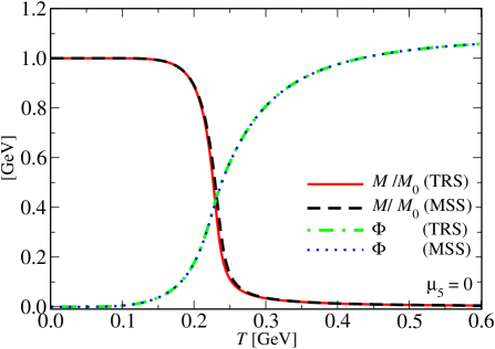
Figure 1: Normalized quark mass $M/M_{0}$ and Polyakov loop $\Phi$ as a function of the temperature at $\mu=\mu_{5}=0$, for both regularization schemes.

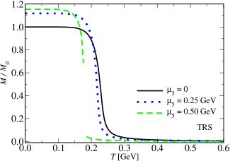
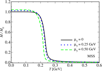
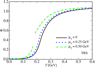
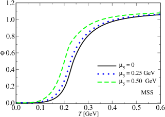
Figure 2: Normalized quark mass $M/M_{0}$ and Polyakov loop $\Phi$ in the TRS case [panels (a) and (c)] and in the MSS case [panels (b) and (d)] as functions of the temperature and for different values of $\mu_{5}$.

To motivate and emphasize the importance of the correct separation of medium contributions in the presence of $\mu_{5}$, we compare the results predicted by both schemes for the chiral density $\langle n_{5}\rangle$. From chiral perturbation theory (ChPT), the QCD partition function in the presence of $\mu_{5}$ is modified to Astrakhantsev:2019wnp :

$$Z(\mu_{5})=Z_{\text{Q}CD}\exp\left[\beta VN_{f}f_{\pi}^{2}\mu_{5}^{2}\right],$$ (25)

where $Z_{\text{Q}CD}$ is the finite-temperature QCD partition function. From this modified partition function one obtains for average of $\langle n_{5}\rangle$:

$$\langle n_{5}\rangle=\frac{1}{\beta V}\frac{\partial\log[Z(\mu_{5})]}{\partial\mu_{5}}=2N_{f}f_{\pi}^{2}\mu_{5}\,.$$ (26)

from which one concludes that $\langle n_{5}\rangle$ is a linearly increasing function of $\mu_{5}$ with with slope $4f_{\pi}^{2}$ in the two-flavor case. Within NJL model, the chiral density can be evaluated from Eq. (7) as

$$\langle n_{5}\rangle=-\frac{\partial\Omega}{\partial\mu_{5}}\,,$$ (27)

which leads to:

$$\langle n_{5}\rangle^{\mathrm{TRS}}=2N_{c}\sum_{s=\pm 1}\int\limits_{0}^{\Lambda}\frac{dp\leavevmode\nobreak\ p^{2}}{2\pi^{2}}\frac{s(|\mathbf{p}|+s\mu_{5})}{\sqrt{(|\mathbf{p}|+s\mu_{5})^{2}+M^{2}}}.$$ (28)

From this result, it is impossible to establish any connection with the ChPT prediction since the $\mu_{5}$ effect is being regularized together with the logarithmic divergence in the momentum integral. For the MSS, on the other hand, the derivative of Eq. (24) results in

$$\langle n_{5}\rangle^{\mathrm{MSS}}=4N_{c}\left[M^{2}I_{\mathrm{log}}(M_{0})-\frac{M^{2}}{4\pi^{2}}\ln\left(\frac{M^{2}}{M_{0}^{2}}\right)\right]\mu_{5}\,,$$

(29)

which is a linear function of $\mu_{5}$ and agrees with the linear behavior predicted by ChPT. Moreover, the slope is precisely the one predicted by ChPT, $4f_{\pi}^{2}$, as we show next. To this end, we follow the works related to the origin of the MSS, referred to as Implicit Regularization Scheme Battistel:1998tj ; Farias:2005cr . Specifically, the authors of those references showed that

$$i\tilde{I}_{\text{log}}(M^{2})=-\frac{f_{\pi}^{2}}{12M^{2}}\,.$$ (30)

In this equation, $\tilde{I}_{\text{log}}(M^{2})$ is defined in Minkowski space as

$$\tilde{I}_{\text{log}}(M^{2})=\int_{\Lambda}\frac{d^{4}k}{(2\pi)^{4}}\frac{1}{(k_{0}^{2}-k^{2}-M^{2})^{2}}\,,$$ (31)

at an arbitrary mass scale $M$, which can still be a function of $\mu_{5}$. We note that $4i\tilde{I}_{\text{log}}(x^{2})=I_{\text{log}}(x^{2})$. This definition is valid at any mass scale $M$, and can be expressed in terms of the vacuum quark mass, $M_{0}$, using the identity:

$$\tilde{I}_{\text{log}}(M^{2})=\tilde{I}_{\text{log}}(M_{0}^{2})-\frac{i}{(4\pi)^{2}}\ln\left(\frac{M^{2}}{M_{0}^{2}}\right)\,.$$ (32)

This allows us to rewrite Eq. (29) as:

$$\langle n_{5}\rangle^{\mathrm{MSS}} = -16N_{c}M^{2}i\tilde{I}_{\mathrm{log}}(M^{2})\mu_{5}{\color[rgb]{0,0,1}.}$$ (33)

With the use of $f_{\pi}^{2}$ from Eq. (30) and taking $N_{c}=3$, leads to:

$$\langle n_{5}\rangle^{\mathrm{MSS}}=4f_{\pi}^{2}\mu_{5}\,,$$ (34)

which proves the ChPT result.

In Fig. 3 we show the TRS and MSS results for $\langle n_{5}\rangle\times\mu_{5}$ at zero temperature. Although it is clear that in this limit the contributions of the Polyakov loop vanish, it is interesting to see that the TRS predicts a plateau for large values of $\mu_{5}$. However, with the MSS we obtain a linear increase of the chiral density with $\mu_{5}$, which is consistent with ChPT predictions and lattice QCD simulation results for heavy pions Astrakhantsev:2019wnp . Although the NJL model parameters used in this work were determined at the physical value of $m_{\pi}$, the linear behavior in MSS is obtained directly from the derivative of Eq. (24) with respect to $\mu_{5}$ and it is not affected by different parametrizations of the model. The linear behavior of $\langle n_{5}\rangle$ as a function of $\mu_{5}$ and the correct prediction of the slope when using the MSS are some of the main results of this paper. In the next section we will explore more thoroughly the thermodynamics of the model and the differences produced by TRS and MSS.

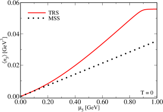
Figure 3: Chiral density from Eq. (27) as a function of $\mu_{5}$ at $T=0$, comparing TRS (left) and MSS (right).

III Numerical Results at zero quark chemical potential

In the PNJL model at $\mu=0$, we have two different (pseudo)critical temperatures, $T_{\rm pc}^{c}$ and $T_{\rm pc}^{d}$, for the chiral and deconfinement transitions, respectively. For both cases, the symmetry is only partially restored (the transitions are crossovers), with the (pseudo)critical values determined by the concavity change of the curves, i.e., by the position of the peak of the first derivatives of $M$ and $\Phi$ with respect to $T$:

$$\left.\frac{\partial^{2}M}{\partial T^{2}}\right|_{T=T_{\rm pc}^{c}}=\left.\frac{\partial^{2}\Phi}{\partial T^{2}}\right|_{T=T_{\rm pc}^{d}}=0.$$ (35)

Recall that the correct order parameter for the chiral transition is the quark condensate, $\langle\bar{q}q\rangle$. However, given its linear relation with the effective quark mass, one may analyze the chiral symmetry restoration through the evolution of $M$ with the temperature and/or with the chemical potential without loss of generality. The phase diagrams in the $T\times\mu_{5}$ plane for the chiral and deconfinement transitions are shown in Fig. 4. The values of the pseudocritical temperatures at $\mu_{5}=0$, $T_{\rm pc}(0)$, are given in Tab. 2 for both regularization schemes.

Table 2: Values of pseudocritical temperatures for chiral ($T_{\rm pc}^{c}$) and deconfinement ($T_{\rm pc}^{d}$) phase transitions.

	$T_{\rm pc}^{c}$ (GeV)	$T_{\rm pc}^{d}$ (GeV)
TRS	0.229	0.225
MSS	0.233	0.227

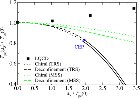
Figure 4: Phase diagrams in the plane $T\times\mu_{5}$ for chiral restoration and deconfinement, comparing lattice results from Ref. Braguta:2015owi , TRS and MSS. The TRS predicts a smooth crossover for both transitions for $\mu_{5}\lesssim 2T_{\rm pc}(0)$, represented by a dotted (chiral) and dashed (deconfinement) lines, succeeding by a first-order transition represented by the solid lines. The MSS results do not present a CEP, but both pseudocritical temperatures are decreasing functions of $\mu_{5}$.

Recent lattice simulations predict a continuous and smooth increasing behavior of the order parameters with $\mu_{5}$ for both the chiral and deconfinement transitions. In addition, the values for $T_{\rm pc}^{c}$ and $T_{\rm pc}^{d}$ are approximately the same Braguta:2015owi . These results are represented by the squared dots in Fig. 4. However, one can see that the PNJL model in the presence of a chiral imbalance using the standard form for the fit of Polyakov loop, given by Eq. (5), is not able to reproduce the lattice QCD behavior. Although the MSS does not predict a critical end point (CEP) as the standard NJL model does Farias:2016let , both schemes lead to decreasing functions of the pseudocritical temperatures with $\mu_{5}$. We have also observed a similar behavior with other Polyakov loop parametrizations commonly considered in the literature. In all available parameterizations, even when using the MSS the pseudocritical temperatures are always decreasing functions of the chiral chemical potential. Our proposal here is that, in order to obtain results in agreement with the lattice results for the pseudocritical temperatures, these parameterizations need to be changed so that they not only depend on the temperature, but also depend on $\mu_{5}$. Thus, we propose an explicit redefinition of the Polyakov loop potential such as to include an explicit dependence of this function with $\mu_{5}$, i.e., $\mathcal{U}(\Phi,T)\to\mathcal{U}(\Phi,T,\mu_{5})$. Still working with the parametrization of the form in Eq. (7), we propose modifying the coefficient of $\Phi\Phi^{\dagger}$ in the potential $\mathcal{U}$ as follows:

$$\mathcal{U}(\Phi,T,\mu_{5}) = T^{4}\bigg{[}-\frac{\bar{b}_{2}(T,\mu_{5})}{2}\Phi\Phi^{\dagger}$$ (36)

$$- \frac{b_{3}}{6}(\Phi^{3}+{\Phi^{\dagger}}^{3})+\frac{b_{4}}{4}(\Phi\Phi^{\dagger})^{2}\bigg{]},$$

in which

$$\bar{b}_{2}(T,\mu_{5}) = a_{0}+a_{1}\left(\frac{T_{0}}{T}\right)+a_{2}\left(\frac{T_{0}}{T}\right)^{2}+a_{3}\left(\frac{T_{0}}{T}\right)^{3}$$ (37)

$$+ k_{1}\left(\frac{\mu_{5}}{T}\right)+k_{2}\left(\frac{\mu_{5}}{T}\right)^{2}+k_{3}\left(\frac{\mu_{5}}{T}\right)^{3}\,.$$

To obtain the MSS results presented in the remainder of this paper we have used $k_{1}=0.08602,k_{2}=-1.39646$ and $k_{3}=0.3381$. These values of constants can be seen to be the fitting values needed to reproduce the lattice results when a chiral chemical potential is present. Note that we have chosen a polynomial dependence on $\mu_{5}$ similar to the one on $T$ of the coeffecient $b_{2}$. We note that a plethora of different parametrization could be used in place of the polynomial we used. We have chosen the simplest one with the aim of showing that the missing ingredient for the models to reproduce lattice QCD simulations is a dependence of the Polyakov loop potential with $\mu_{5}$, in addition to the dependence on $T$.

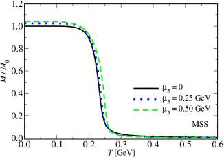
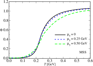
Figure 5: MSS results for the normalized quark mass $M/M_{0}$ on panel (a) and Polyakov loop $\Phi$ on panel (b) as functions of the temperature, for $\mu=0$ and different values of $\mu_{5}$. Results obtained with the redefined Polyakov loop potential as given by Eq. (36).

In Fig. 5 we show the results for the normalized quark mass and Polyakov loop $\Phi$ as functions of the temperature for the MSS, using the newly redefined $\mathcal{U}(\Phi,T,\mu_{5})$ as given in Eq. (36). From this figure one can see that the inflection points in the curves are shifted to the right, which means that the pseudocritical temperatures now increase with $\mu_{5}$. This is the opposite behavior to that observed in Fig. 2. The results for the pseudocritical temperatures as a function of $\mu_{5}$, when using Eq. (36), are shown in Fig. 6. From Fig. 6 one can see that the dependence of the Polyakov potential with the chiral chemical potential enables the PNJL model to reproduce the correct behavior of lattice simulation results and also make the values of $T_{\rm pc}^{c}$ and $T_{\rm pc}^{d}$ closer to each other. Note that if we consider the TRS method instead and by using $\mathcal{U}(\Phi,T,\mu_{5})$ , we still obtain a CEP in the $T\times\mu_{5}$ plane, which is not consistent with the lattice simulations; for this reason, we opted for showing only the MSS results in this case.

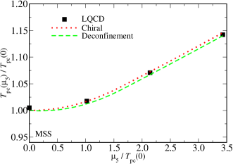
Figure 6: Phase diagrams in the plane $T\times\mu_{5}$ for chiral restoration and deconfinement, comparing lattice results from Ref. Braguta:2015owi and MSS, including a dependence with $\mu_{5}$ on the Polyakov loop potential, as given in Eq. (36). The dotted and dashed lines are the MSS results for chiral and deconfinement transitions, respectively, while large dots are lattice results.

III.1 Thermodynamic quantities

Next, we study the thermodynamics of the PNJL model at $\mu=0$, comparing the TRS with $\mathcal{U}(\Phi,T)$ and MSS with $\mathcal{U}(\Phi,T,\mu_{5})$. From the thermodynamic potential given in Eq.(7) it is possible to compute several thermodynamic quantities, starting from the normalized pressure:

$$p_{N}(M,\bar{M},\Phi,\Phi^{\dagger},T,\mu,\mu_{5})= -\bigg{[}\Omega(M,\Phi,\Phi^{\dagger},T,\mu,\mu_{5})$$

$$-\Omega(\bar{M},0,\mu,\mu_{5})\bigg{]},$$ (38)

where $\bar{M}\equiv M(\mu,\mu_{5})$ is defined at finite chemical potentials but zero temperature. For simplicity, we will omit the functional dependencies in all thermodynamic quantities. The entropy $s$ and energy $\varepsilon$ densities are defined at fixed $\mu_{5}$, respectively as

$$s=\left.\frac{\partial p_{N}}{\partial T}\right|_{\mu_{5}},$$ (39)

$$\varepsilon=Ts-p_{N}+\mu_{5}\langle n_{5_{N}}\rangle,$$ (40)

where the normalized chiral density $\langle n_{5_{N}}\rangle$ is defined in terms of the normalized pressure as

$$\langle n_{5_{N}}\rangle=\frac{\partial p_{N}}{\partial\mu_{5}}.$$ (41)

Another interesting quantity is the squared speed of sound, also at finite $\mu_{5}$,

$$c_{s}^{2}=\left.\frac{\partial p_{N}}{\partial\varepsilon}\right|_{\mu_{5}}=\frac{s}{C_{v}},$$ (42)

that may be defined in terms of the specific heat as

$$C_{v}=T\frac{\partial s}{\partial T}\,.$$ (43)

It is common to find in the literature an alternative definition of the squared speed of sound, calculated at fixed entropy per baryon $s/n_{B}$. This alternative definition is motivated in the context of heavy ion collisions since the speed of sound is approximately constant in the whole expansion stage of the collision Braun-Munzinger:2015hba . Since we are working at zero quark density, we will use the definition of $c_{s}^{2}$ at finite chiral chemical potential as given in Eq. (42). Finally, we also consider the scaled trace anomaly $\Delta$, also referred to in the literature as “interaction measure”:

$$\Delta=\frac{1}{T^{4}}\left(\varepsilon-3p_{N}\right),$$ (44)

This quantity helps to assess the high temperature limit of the system as provides a measure of the deviation from the scale invariance.

Results for $p_{N}$, $s$, $\epsilon$, $c^{2}_{s}$, and $\Delta$ are shown in Figs 7 and 8. Initially, it is worth mentioning that the results for these thermodynamic quantities converge to the Stefan-Boltzmann limit, i.e. the limit of a gas of noninteracting particles. We recall that the Stefan-Boltzmamm limit of the pressure is given by Costa:2009ae :

$$p_{\mathrm{SB_{qg}}}=T^{4}\left(p_{\mathrm{SB_{g}}}+p_{\mathrm{SB_{q}}}\right),$$ (45)

where

$$p_{\mathrm{SB_{g}}} = \left(N_{c}^{2}-1\right)\frac{\pi^{2}}{45},$$ (46)

$$p_{\mathrm{SB_{q}}} = N_{c}N_{f}\frac{7\pi^{2}}{180},$$ (47)

are the contributions from the gluons and fermions respectively. The Stefan-Boltzmann limits for the other thermodynamic quantities, which are derived from the pressure according to the definitions (39)-(42) given above, and are also identified in Figs. 7 and 8.

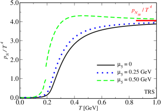
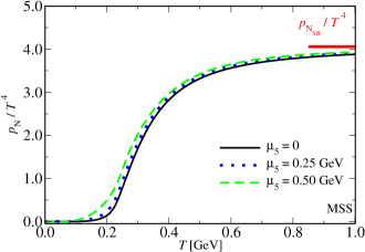
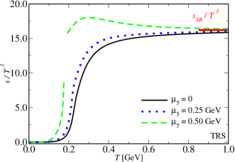
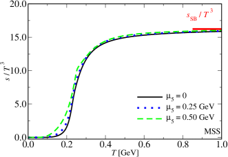
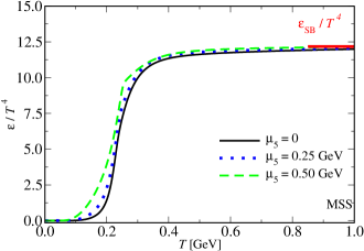
Figure 7: The normalized pressure $p_{N}/T^{4}$, entropy $s/T^{3}$ and energy density $\varepsilon/T^{4}$ as a function of temperature and different values of $\mu_{5}$ (all at $\mu=0$) in the TRS case, panels (a), (c) and (e), respectively and in the MSS case, panels (b), (d) and (f), respectively. All results obtained using $\mathcal{U}(\Phi,T,\mu_{5})$ as given by Eq. (36).

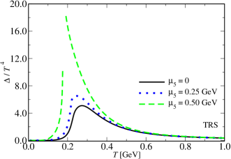
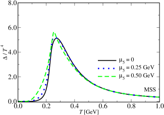
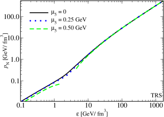
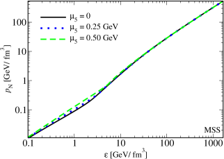
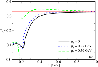
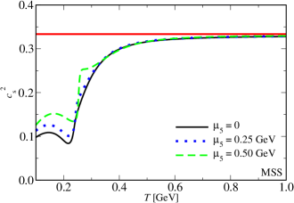
Figure 8: Scaled trace anomaly $\Delta/T^{4}$, equation of state $p_{N}\times\varepsilon$ and sound velocity squared as a function of temperature and different values of $\mu_{5}$ (all at $\mu=0$) in the TRS case, panels (a), (c) and (e), respectively and in the MSS case, panels (b), (d) and (f), respectively. All results obtained using $\mathcal{U}(\Phi,T,\mu_{5})$ as given by Eq. (36).

Figure 7 reveals that all TRS results show a discontinuity for $\mu_{5}>0.44$ GeV at the critical temperature, characteristic of a first-order transition, contrary to the MSS results that predict a crossover. Although both schemes lead to results that converge to the Stefan-Boltzmann limit at high temperatures, the TRS results for the pressure, entropy, and energy density approach this limit from above for $\mu_{5}=0.5$ GeV, for which there is a first-order transition. For the MSS using $\mathcal{U}(\Phi,T,\mu_{5})$, Eq. (36), the curves are less sensitive to the increase of $\mu_{5}$ and converge very fast, however, they can exceed the Stefan-Boltzmann limits for some values of the chiral chemical potential when going beyond $\mu_{5}>0.5$ GeV.

It is known that the scaled trace anomaly $\Delta$ has peaks sharply at the deconfined temperature and has a tail that approaches zero at asymptotically large values of $T$ in pure gauge theories. A similar behavior is obtained for the PNJL model as shown in Fig. 8 for both methods, with the caveat that at $\mu_{5}=0.5$ GeV the TRS curve diverges at the critical temperature. Also in Fig. 8, we show a comparison of the TRS and MSS results for the equation of state (EoS) and the squared speed of sound. From Eq. (42), one can see that $c_{s}^{2}$ represents the slope of the curve $p_{n}\times\varepsilon$ at each temperature value. Once again, the main difference between the curves occurs at $\mu_{5}=0.5$ GeV for TRS, for which the speed of sound goes to zero in the first-order transition region. To express the pressure and energy density for the same temperature range used for $c_{s}^{2}$ it is more convenient to use a logarithmic scale in the EoS plot. This is the reason why the jump at $p_{N}\lesssim$ 0.1 GeV/fm³ appears to be more pronounced than the equivalent discontinuity in the squared speed of sound. On the other hand, the MSS curve does not show a first-order transition; the step-like behavior in the region $0.2\leavevmode\nobreak\ {\rm GeV}\lesssim T\lesssim 0.3\leavevmode\nobreak\ {\rm GeV}$ is related to a continuous change of slope of the EoS in the range $0.8\leavevmode\nobreak\ {\rm GeV/fm}^{3}\lesssim\varepsilon\lesssim 10\leavevmode\nobreak\ {\rm GeV/fm}^{3}$. For the other values of $\mu_{5}$ in both methods, the curves approach the conformal limit of 1/3 at values of $T$ of the order of $0.6$ GeV.

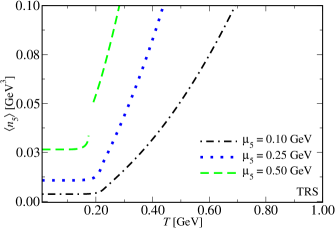
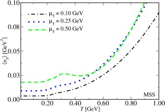
Figure 9: Chiral density from Eq. (27) as a function of the temperature $T$, comparing TRS, on panel (a) and MSS, on panel (b), for different values of $\mu_{5}$.

In Fig. 9 we show the results for the chiral density $\langle n_{5}\rangle$, defined in Eq. (27), in both the TRS and MSS methods and using the redefined Polyakov loop given by Eq. (36). This is the quantity for which the differences between TRS and MSS are more pronounced. In the TRS case, for all the values of $\mu_{5}$ considered, the curves have a similar behavior as a function of temperature: a constant line with a change in concavity at the transition temperature, succeeded by a monotonic increase. For $\mu_{5}=0.5$ GeV this quantity also presents a small jump at $T_{\rm pc}$, characteristic of a first-order transition. In the MSS case, $\langle n_{5}\rangle$ is an increasing function of the temperature for small values of $\mu_{5}$, and shows a small hump in the pseudocritical temperature region for higher values of of $\mu_{5}$. We do not show the results for $\mu_{5}=0$ because $\langle n_{5}\rangle$ is trivially zero in this case.

IV Phase diagram at finite quark chemical potential

Finally, we consider the influence on the phase diagram in the $T\times\mu$ plane of including the dependence on $\mu_{5}$ in the Polyakov loop potential as indicated in Eq. (37). In this case, we have $\Phi\neq\Phi^{\dagger}$ and, instead of Eq. (35), we need to solve

$$\left.\frac{\partial^{2}M}{\partial T^{2}}\right|_{T=T^{c}_{\rm pc}}=\left.\frac{\partial^{2}\Phi}{\partial T^{2}}\right|_{T=T^{\Phi}_{\rm pc}}=\left.\frac{\partial^{2}\Phi^{\dagger}}{\partial T^{2}}\right|_{T=T^{\Phi^{\dagger}}_{\rm pc}}=0.$$ (48)

We define the deconfinement pseudocritical temperature $T_{\rm pc}^{d}$ as the average of $T^{\Phi}_{\rm pc}$ and $T^{\Phi^{\dagger}}_{\rm pc}$:

$$T_{\rm pc}^{d}=\frac{T^{\Phi}_{\rm pc}+T^{\Phi^{\dagger}}_{\rm pc}}{2}\,.$$ (49)

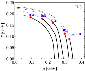
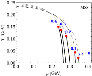
Figure 10: The evolution of the CEP in the space $T\times\mu$, for different values of $\mu_{5}$, comparing TRS, on panel (a), and MSS, on panel (b). Dashed and solid lines correspond to second and first-order transitions, respectively, while the large dot is the CEP. The values of $\mu_{5}$ are presented right above the CEPs, and their values are given in GeV.

Figure 10 shows the evolution of the CEP for different values of $\mu_{5}$. One sees that the CEP is shifted toward lower values of $\mu$ and higher values of $T$ when $\mu_{5}$ increases. The same behavior is observed for TRS using $\mathcal{U}(\Phi,\Phi^{\dagger},T)$ from Eq. (5) and for MSS using $\mathcal{U}(\Phi,\Phi^{\dagger},T,\mu_{5})$ from Eq. (36), although the positions of the critical end points and the slopes of the curves are different for each scheme.

V Conclusions

In this paper, we performed a thorough study within the PNJL model on the differences that the TRS and MSS regularization procedures imply for the thermodynamics of quark matter with chiral imbalance. We have shown that, to reproduce lattice results for the chiral and deconfinement pseudocritical temperatures as a function of the chiral chemical potential $\mu_{5}$, it is necessary to include a $\mu_{5}$-dependece in the parametrization of the quadratic $\Phi^{\dagger}\Phi$ term in Polyakov loop potential, in addition to the usual temperature dependence. We have proposed a polynomial dependence analogous to that in terms of temperature. In addition to reproducing the lattice results for values of the pseudocritical temperatures, the proposed parametrization also reproduces the increase of those temperatures with $\mu_{5}$, indicating that such a $\mu_{5}$ dependence in the Polyakov loop potential may be the missing ingredient in the traditional PNJL models. We have studied the changes caused by this new parametrization of the Polyakov loop potential in various thermodynamic quantities, and also contrasted the results predicted by the TRS and MSS regularization procedures. In particular, we have shown that the combined use of the new parametrization of the Polyakov loop potential and the MSS procedure leads to consistent results that agree with those of lattice simulations.

VI Acknowledgements

This work was partially supported by Conselho Nacional de Desenvolvimento Científico e Tecnológico (CNPq), Grants No. 312032/2023-4 (R.L.S.F.), 307286/2021-5 (R.O.R.); Fundação de Amparo à Pesquisa do Estado do Rio Grande do Sul (FAPERGS), Grants Nos. 19/2551-0000690-0 and 19/2551-0001948-3 (R.L.S.F.), and 23/2551-0000791-6 and 23/2551-0001591-9 (D.C.D.); Fundação Carlos Chagas Filho de Amparo à Pesquisa do Estado do Rio de Janeiro (FAPERJ), Grant No. E-26/201.150/2021 (R.O.R.); Coordenação de Aperfeiçoamento de Pessoal de Nível Superior - Brasil (CAPES) - Finance Code 001 (F.X.A.). The work is also part of the project Instituto Nacional de Ciência e Tecnologia - Física Nuclear e Aplicações (INCT - FNA), Grant No. 464898/2014-5 and supported by the Serrapilheira Institute (grant number Serra - 2211-42230).

References

- (1) K. Fukushima, D. E. Kharzeev and H. J. Warringa, The Chiral Magnetic Effect, Phys. Rev. D 78, 074033 (2008) doi:10.1103/PhysRevD.78.074033 [arXiv:0808.3382 [hep-ph]].
- (2) A. Vilenkin, EQUILIBRIUM PARITY VIOLATING CURRENT IN A MAGNETIC FIELD, Phys. Rev. D 22, 3080-3084 (1980) doi:10.1103/PhysRevD.22.3080
- (3) D. T. Son and A. R. Zhitnitsky, Quantum anomalies in dense matter, Phys. Rev. D 70, 074018 (2004) doi:10.1103/PhysRevD.70.074018 [arXiv:hep-ph/0405216 [hep-ph]].
- (4) M. A. Metlitski and A. R. Zhitnitsky, Anomalous axion interactions and topological currents in dense matter, Phys. Rev. D 72, 045011 (2005) doi:10.1103/PhysRevD.72.045011 [arXiv:hep-ph/0505072 [hep-ph]].
- (5) D. T. Son and P. Surowka, Hydrodynamics with Triangle Anomalies, Phys. Rev. Lett. 103, 191601 (2009) doi:10.1103/PhysRevLett.103.191601 [arXiv:0906.5044 [hep-th]].
- (6) A. Vilenkin, MACROSCOPIC PARITY VIOLATING EFFECTS: NEUTRINO FLUXES FROM ROTATING BLACK HOLES AND IN ROTATING THERMAL RADIATION, Phys. Rev. D 20, 1807-1812 (1979) doi:10.1103/PhysRevD.20.1807
- (7) N. Banerjee, J. Bhattacharya, S. Bhattacharyya, S. Dutta, R. Loganayagam and P. Surowka, Hydrodynamics from charged black branes, JHEP 01, 094 (2011) doi:10.1007/JHEP01(2011)094 [arXiv:0809.2596 [hep-th]].
- (8) K. Landsteiner, E. Megias and F. Pena-Benitez, Gravitational Anomaly and Transport, Phys. Rev. Lett. 107, 021601 (2011) doi:10.1103/PhysRevLett.107.021601 [arXiv:1103.5006 [hep-ph]].
- (9) D. Suenaga, K. Suzuki, Y. Araki and S. Yasui, Kondo effect driven by chirality imbalance, Phys. Rev. Res. 2, no.2, 023312 (2020) doi:10.1103/PhysRevResearch.2.023312 [arXiv:1912.12669 [hep-ph]].
- (10) D. E. Kharzeev and H. U. Yee, Chiral Magnetic Wave, Phys. Rev. D 83, 085007 (2011) doi:10.1103/PhysRevD.83.085007 [arXiv:1012.6026 [hep-th]].
- (11) M. N. Chernodub, Chiral Heat Wave and mixing of Magnetic, Vortical and Heat waves in chiral media, JHEP 01, 100 (2016) doi:10.1007/JHEP01(2016)100 [arXiv:1509.01245 [hep-th]].
- (12) N. Yamamoto, Chiral Alfvén Wave in Anomalous Hydrodynamics, Phys. Rev. Lett. 115, no.14, 141601 (2015) doi:10.1103/PhysRevLett.115.141601 [arXiv:1505.05444 [hep-th]].
- (13) K. Rajagopal and A. V. Sadofyev, Chiral drag force, JHEP 10, 018 (2015) doi:10.1007/JHEP10(2015)018 [arXiv:1505.07379 [hep-th]].
- (14) A. V. Sadofyev and Y. Yin, The charmonium dissociation in an “anomalous wind”, JHEP 01, 052 (2016) doi:10.1007/JHEP01(2016)052 [arXiv:1510.06760 [hep-th]].
- (15) D. E. Kharzeev, J. Liao and P. Tribedy, Chiral Magnetic Effect in Heavy Ion Collisions: The Present and Future, [arXiv:2405.05427 [nucl-th]].
- (16) Z. Song, J. Zhao, Z. Fang and X. Dai, Detecting the chiral magnetic effect by lattice dynamics in Weyl semimetals, Phys. Rev. B 94, no.21, 214306 (2016) doi:10.1103/PhysRevB.94.214306 [arXiv:1609.05442 [cond-mat.mtrl-sci]].
- (17) V. V. Braguta, M. I. Katsnelson, A. Y. Kotov and A. M. Trunin, Catalysis of Dynamical Chiral Symmetry Breaking by Chiral Chemical Potential in Dirac semimetals, Phys. Rev. B 100, no.8, 085117 (2019) doi:10.1103/PhysRevB.100.085117 [arXiv:1904.07003 [cond-mat.str-el]].
- (18) K. Kamada, N. Yamamoto and D. L. Yang, Chiral effects in astrophysics and cosmology, Prog. Part. Nucl. Phys. 129, 104016 (2023) doi:10.1016/j.ppnp.2022.104016 [arXiv:2207.09184 [astro-ph.CO]].
- (19) J. Charbonneau and A. Zhitnitsky, Topological Currents in Neutron Stars: Kicks, Precession, Toroidal Fields, and Magnetic Helicity, JCAP 08, 010 (2010) doi:10.1088/1475-7516/2010/08/010 [arXiv:0903.4450 [astro-ph.HE]].
- (20) A. Ohnishi and N. Yamamoto, Magnetars and the Chiral Plasma Instabilities, [arXiv:1402.4760 [astro-ph.HE]].
- (21) L. K. Yang, X. F. Luo, J. Segovia and H. S. Zong, A Brief Review of Chiral Chemical Potential and Its Physical Effects, Symmetry 12, no.12, 2095 (2020) doi:10.3390/sym12122095
- (22) T. G. Khunjua, K. G. Klimenko and R. N. Zhokhov, Influence of chiral chemical potential 5 on phase structure of the two-color quark matter, Phys. Rev. D 106, no.4, 045008 (2022) doi:10.1103/PhysRevD.106.045008 [arXiv:2105.04952 [hep-ph]].
- (23) T. G. Khunjua, K. G. Klimenko and R. N. Zhokhov, Chiral imbalanced hot and dense quark matter: NJL analysis at the physical point and comparison with lattice QCD, Eur. Phys. J. C 79, no.2, 151 (2019) doi:10.1140/epjc/s10052-019-6654-2 [arXiv:1812.00772 [hep-ph]].
- (24) T. G. Khunjua, K. G. Klimenko and R. N. Zhokhov, Dense Baryonic Matter and Applications of QCD Phase Diagram Dualities, Particles 3, no.1, 62-79 (2020) doi:10.3390/particles3010006 [arXiv:2005.04641 [hep-ph]].
- (25) T. G. Khunjua, K. G. Klimenko and R. N. Zhokhov, Dualities in dense quark matter with isospin, chiral, and chiral isospin imbalance in the framework of the large-Nc limit of the NJL4 model, Phys. Rev. D 98, no.5, 054030 (2018) doi:10.1103/PhysRevD.98.054030 [arXiv:1804.01014 [hep-ph]].
- (26) M. Ruggieri, Z. Y. Lu and G. X. Peng, Influence of chiral chemical potential, parallel electric, and magnetic fields on the critical temperature of QCD, Phys. Rev. D 94, no.11, 116003 (2016) doi:10.1103/PhysRevD.94.116003 [arXiv:1608.08310 [hep-ph]].
- (27) V. V. Braguta, E. M. Ilgenfritz, A. Y. Kotov, B. Petersson and S. A. Skinderev, Study of QCD Phase Diagram with Non-Zero Chiral Chemical Potential, Phys. Rev. D 93, no.3, 034509 (2016) doi:10.1103/PhysRevD.93.034509 [arXiv:1512.05873 [hep-lat]].
- (28) V. V. Braguta, V. A. Goy, E. M. Ilgenfritz, A. Y. Kotov, A. V. Molochkov, M. Muller-Preussker and B. Petersson, Two-Color QCD with Non-zero Chiral Chemical Potential, JHEP 06, 094 (2015) doi:10.1007/JHEP06(2015)094 [arXiv:1503.06670 [hep-lat]].
- (29) M. Ruggieri, The Critical End Point of Quantum Chromodynamics Detected by Chirally Imbalanced Quark Matter, Phys. Rev. D 84, 014011 (2011) doi:10.1103/PhysRevD.84.014011 [arXiv:1103.6186 [hep-ph]].
- (30) K. Fukushima, M. Ruggieri and R. Gatto, Chiral magnetic effect in the PNJL model, Phys. Rev. D 81, 114031 (2010) doi:10.1103/PhysRevD.81.114031 [arXiv:1003.0047 [hep-ph]].
- (31) J. Chao, P. Chu and M. Huang, Inverse magnetic catalysis induced by sphalerons, Phys. Rev. D 88, 054009 (2013) doi:10.1103/PhysRevD.88.054009 [arXiv:1305.1100 [hep-ph]].
- (32) L. Yu, H. Liu and M. Huang, Spontaneous generation of local CP violation and inverse magnetic catalysis, Phys. Rev. D 90, no.7, 074009 (2014) doi:10.1103/PhysRevD.90.074009 [arXiv:1404.6969 [hep-ph]].
- (33) L. Yu, H. Liu and M. Huang, Effect of the chiral chemical potential on the chiral phase transition in the NJL model with different regularization schemes, Phys. Rev. D 94, no.1, 014026 (2016) doi:10.1103/PhysRevD.94.014026 [arXiv:1511.03073 [hep-ph]].
- (34) M. N. Chernodub and A. S. Nedelin, Phase diagram of chirally imbalanced QCD matter, Phys. Rev. D 83, 105008 (2011) doi:10.1103/PhysRevD.83.105008 [arXiv:1102.0188 [hep-ph]].
- (35) V. V. Braguta and A. Y. Kotov, Catalysis of Dynamical Chiral Symmetry Breaking by Chiral Chemical Potential, Phys. Rev. D 93, no.10, 105025 (2016) doi:10.1103/PhysRevD.93.105025 [arXiv:1601.04957 [hep-th]].
- (36) M. Hanada and N. Yamamoto, Universality of phase diagrams in QCD and QCD-like theories, PoS LATTICE2011, 221 (2011) doi:10.22323/1.139.0221 [arXiv:1111.3391 [hep-lat]].
- (37) B. Wang, Y. L. Wang, Z. F. Cui and H. S. Zong, Effect of the chiral chemical potential on the position of the critical endpoint, Phys. Rev. D 91, no.3, 034017 (2015) doi:10.1103/PhysRevD.91.034017
- (38) S. S. Xu, Z. F. Cui, B. Wang, Y. M. Shi, Y. C. Yang and H. S. Zong, Chiral phase transition with a chiral chemical potential in the framework of Dyson-Schwinger equations, Phys. Rev. D 91, no.5, 056003 (2015) doi:10.1103/PhysRevD.91.056003 [arXiv:1505.00316 [hep-ph]].
- (39) C. Shi, X. T. He, W. B. Jia, Q. W. Wang, S. S. Xu and H. S. Zong, Chiral transition and the chiral charge density of the hot and dense QCD matter, JHEP 06, 122 (2020) doi:10.1007/JHEP06(2020)122 [arXiv:2004.09918 [hep-ph]].
- (40) Y. L. Tian, Z. F. Cui, B. Wang, Y. M. Shi, Y. C. Yang and H. S. Zong, Dyson–Schwinger Equations of Chiral Chemical Potential, Chin. Phys. Lett. 32, no.8, 081101 (2015) doi:10.1088/0256-307X/32/8/081101
- (41) Z. F. Cui, I. C. Cloet, Y. Lu, C. D. Roberts, S. M. Schmidt, S. S. Xu and H. S. Zong, Critical endpoint in the presence of a chiral chemical potential, Phys. Rev. D 94, 071503 (2016) doi:10.1103/PhysRevD.94.071503 [arXiv:1604.08454 [nucl-th]].
- (42) M. Frasca, Nonlocal Nambu–Jona-Lasinio model and chiral chemical potential, Eur. Phys. J. C 78, no.9, 790 (2018) doi:10.1140/epjc/s10052-018-6200-7 [arXiv:1602.04654 [hep-ph]].
- (43) M. Ruggieri and G. X. Peng, Critical Temperature of Chiral Symmetry Restoration for Quark Matter with a Chiral Chemical Potential, J. Phys. G 43, no.12, 125101 (2016) doi:10.1088/0954-3899/43/12/125101 [arXiv:1602.05250 [hep-ph]].
- (44) M. Ruggieri, M. N. Chernodub and Z. Y. Lu, Topological susceptibility, divergent chiral density and phase diagram of chirally imbalanced QCD medium at finite temperature, Phys. Rev. D 102, no.1, 014031 (2020) doi:10.1103/PhysRevD.102.014031 [arXiv:2004.09393 [hep-ph]].
- (45) R. L. Liu, M. Y. Lai, C. Shi and H. S. Zong, Finite volume effects on QCD susceptibilities with a chiral chemical potential, Phys. Rev. D 102, no.1, 014014 (2020) doi:10.1103/PhysRevD.102.014014
- (46) R. L. Liu and H. S. Zong, QCD susceptibilities in the presence of the chiral chemical potential, Mod. Phys. Lett. A 35, no.16, 2050137 (2020) doi:10.1142/S0217732320501370
- (47) L. K. Yang, X. Luo and H. S. Zong, QCD phase diagram in chiral imbalance with self-consistent mean field approximation, Phys. Rev. D 100, no.9, 094012 (2019) doi:10.1103/PhysRevD.100.094012 [arXiv:1910.13185 [nucl-th]].
- (48) Z. Pan, Z. F. Cui, C. H. Chang and H. S. Zong, Finite-volume effects on phase transition in the Polyakov-loop extended Nambu–Jona-Lasinio model with a chiral chemical potential, Int. J. Mod. Phys. A 32, no.13, 1750067 (2017) doi:10.1142/S0217751X17500671 [arXiv:1611.07370 [hep-ph]].
- (49) Y. Lu, Z. F. Cui, Z. Pan, C. H. Chang and H. S. Zong, QCD phase diagram with a chiral chemical potential, Phys. Rev. D 93, no.7, 074037 (2016) doi:10.1103/PhysRevD.93.074037
- (50) M. Ruggieri and G. X. Peng, Critical Temperature of Chiral Symmetry Restoration for Quark Matter with a Chiral Chemical Potential, [arXiv:1602.03651 [hep-ph]].
- (51) D. Espriu, A. Gómez Nicola and A. Vioque-Rodríguez, Chiral perturbation theory for nonzero chiral imbalance, JHEP 06, 062 (2020) doi:10.1007/JHEP06(2020)062 [arXiv:2002.11696 [hep-ph]].
- (52) A. Gómez Nicola, P. Roa-Bravo and A. Vioque-Rodríguez, Pion scattering, light resonances, and chiral symmetry restoration at nonzero chiral imbalance and temperature, Phys. Rev. D 109, no.3, 034011 (2024) doi:10.1103/PhysRevD.109.034011 [arXiv:2311.01917 [hep-ph]].
- (53) A. A. Andrianov, V. A. Andrianov and D. Espriu, Chiral perturbation theory vs. Linear Sigma Model in a chiral imbalance medium, Particles 3, no.1, 15-22 (2020) doi:10.3390/particles3010002 [arXiv:1908.09118 [hep-th]].
- (54) R. L. S. Farias, D. C. Duarte, G. Krein and R. O. Ramos, Thermodynamics of quark matter with a chiral imbalance, Phys. Rev. D 94, no.7, 074011 (2016) doi:10.1103/PhysRevD.94.074011 [arXiv:1604.04518 [hep-ph]].
- (55) C. Ratti, M. A. Thaler and W. Weise, Phases of QCD: Lattice thermodynamics and a field theoretical model, Phys. Rev. D 73, 014019 (2006) doi:10.1103/PhysRevD.73.014019 [arXiv:hep-ph/0506234 [hep-ph]].
- (56) K. Fukushima and V. Skokov, Polyakov loop modeling for hot QCD, Prog. Part. Nucl. Phys. 96, 154-199 (2017) doi:10.1016/j.ppnp.2017.05.002 [arXiv:1705.00718 [hep-ph]].
- (57) P. Costa, H. Hansen, M. C. Ruivo and C. A. de Sousa, How parameters and regularization affect the PNJL model phase diagram and thermodynamic quantities, Phys. Rev. D 81, 016007 (2010) doi:10.1103/PhysRevD.81.016007 [arXiv:0909.5124 [hep-ph]].
- (58) J. P. Carlomagno, D. G. Dumm and N. N. Scoccola, Isospin asymmetric matter in a nonlocal chiral quark model, Phys. Rev. D 104, no.7, 074018 (2021) doi:10.1103/PhysRevD.104.074018 [arXiv:2107.02022 [hep-ph]].
- (59) B. J. Schaefer, M. Wagner and J. Wambach, Thermodynamics of (2+1)-flavor QCD: Confronting Models with Lattice Studies, Phys. Rev. D 81, 074013 (2010) doi:10.1103/PhysRevD.81.074013 [arXiv:0910.5628 [hep-ph]].
- (60) B. S. Lopes, S. S. Avancini, A. Bandyopadhyay, D. C. Duarte and R. L. S. Farias, Hot QCD at finite isospin density: Confronting the SU(3) Nambu–Jona-Lasinio model with recent lattice data, Phys. Rev. D 103, no.7, 076023 (2021) doi:10.1103/PhysRevD.103.076023 [arXiv:2102.02844 [hep-ph]].
- (61) R. L. S. Farias, G. Dallabona, G. Krein and O. A. Battistel, Cutoff-independent regularization of four-fermion interactions for color superconductivity, Phys. Rev. C 73, 018201 (2006) doi:10.1103/PhysRevC.73.018201 [arXiv:hep-ph/0510145 [hep-ph]].
- (62) D. C. Duarte, R. L. S. Farias and R. O. Ramos, Regularization issues for a cold and dense quark matter model in equilibrium, Phys. Rev. D 99, no.1, 016005 (2019) doi:10.1103/PhysRevD.99.016005 [arXiv:1811.10598 [hep-ph]].
- (63) N. Y. Astrakhantsev, V. V. Braguta, A. Y. Kotov, D. D. Kuznedelev and A. A. Nikolaev, Lattice study of QCD at finite chiral density: topology and confinement, Eur. Phys. J. A 57, no.1, 15 (2021) doi:10.1140/epja/s10050-020-00326-2 [arXiv:1902.09325 [hep-lat]].
- (64) O. A. Battistel and M. C. Nemes, Consistency in regularizations of the gauged NJL model at one loop level, Phys. Rev. D 59, 055010 (1999) doi:10.1103/PhysRevD.59.055010 [arXiv:hep-th/9811154 [hep-th]].
- (65) P. Braun-Munzinger, V. Koch, T. Schäfer and J. Stachel, Properties of hot and dense matter from relativistic heavy ion collisions, Phys. Rept. 621, 76-126 (2016) doi:10.1016/j.physrep.2015.12.003 [arXiv:1510.00442 [nucl-th]].