Stability of stationary states for mean field models with multichromatic interaction potentials

Abstract

We consider weakly interacting diffusions on the torus, for multichromatic interaction potentials. We consider interaction potentials that are not $H$-stable, leading to phase transitions in the mean field limit. We show that the mean field dynamics can exhibit multipeak stationary states, where the number of peaks is related to the number of nonzero Fourier modes of the interaction. We also consider the effect of a confining potential on the structure of non-uniform steady states. We approach the problem by means of analysis, perturbation theory and numerical simulations for the interacting particle systems and the PDEs.

¹Department of Mathematics, Imperial College London, London SW7 2AZ, UK.
benedetta.bertoli21@imperial.ac.uk and pavl@ic.ac.uk

²School of Mathematics and the Maxwell Institute for Mathematical Sciences, University of Edinburgh, Edinburgh EH9 3FD, UK. b.goddard@ed.ac.uk

1 Introduction

Nonlinear and nonlocal Fokker-Planck (advection-diffusion) equations appear in several applications, including stellar dynamics [6], plasma physics [2], mathematical biology [30, 33], active matter [32], biophysics [18][Sec 5.3], nematic liquid crystals [11] and models for opinion formation [22]. Such PDEs can exhibit nontrivial, i.e. non-uniform, stationary states, describing collective behaviour and the emergence of coherent structures, as an effect of interactions between agents at the microscale. In recent years, great progress has been made towards the understanding of the emergence of such collective behaviour. The purpose of this paper is to study the creation and stability of multimodal/multipeak stationary states for nonlinear, nonlocal Fokker-Planck equations on the torus.

In this paper, we will consider nonlinear, nonlocal Fokker-Planck equations of the form

$$\frac{\partial\rho}{\partial t}=\beta^{-1}\Delta\rho+\nabla\cdot(\nabla V\rho)+\nabla\cdot((\nabla W\star\rho)\rho),\quad\rho(x,0)=\rho_{0}(x),$$ (1)

on $\mathbb{T}^{d}:=[0,2\pi]^{d}$ with periodic boundary conditions. We will focus on the one dimensional problem. Here $\rho$ denotes the density/distribution function, $\rho_{0}$ the initial condition, $\beta$ the inverse temperature and $V$ and $W$ the confining and (symmetric) interaction potentials, respectively. Examples of dynamics described by (1) are the Haken-Kelso-Bunz model from biophysics [18] with $V(x)=-\alpha\cos(x)-\gamma\cos(2x)$ and $W(x)=-K\cos(x)$, where $\alpha,\,\gamma,K$ are constants. We also mention the XY ($O(2)$) model with an external magnetic field that was studied in [14], corresponding to $V(x)=-\alpha\cos(x)$ and $W(x)=-K\cos(x)$, as well as the the noisy Kuramoto/Brownian mean field model [5, 10], $V\equiv 0$ and $W(x)=-\cos(x)$ and the noisy Hegselmann-Krause model for opinion dynamics [22, 19]. Several additional examples can be found in [9][Sec. 6]. A very nice presentation of the nonlinear Fokker-Planck equation on the torus from a theoretical physics perspective can be found in [18, Sec. 5.3] and in [10].

As is well known [9], the McKean-Vlasov PDE has a gradient structure:

$$\partial_{t}\rho=\nabla\cdot\left(\rho\nabla\frac{\delta\mathcal{F}}{\delta\rho}\right),$$ (2)

where $\mathcal{F}$ denotes the free energy

$$\mathcal{F}(\rho)=\beta^{-1}\int_{\mathbb{T}^{d}}\rho(x)\log(\rho(x))\,\mathrm{d}x+\int_{\mathbb{T}^{d}}V(x)\rho(x)\,\mathrm{d}x+\frac{1}{2}\int_{\mathbb{T}^{d}}\int_{\mathbb{T}^{d}}W(x-y)\rho(x)\rho(y)\,\mathrm{d}x\,\mathrm{d}y.$$ (3)

Stationary states of the mean field dynamics can be characterized as critical points of the free energy [9]. The main goal of this paper is to study the dynamical stability of such states, in particular of stationary states that describe collective, organized behaviour.

Stationary states of the McKean-Vlasov PDE satisfy the Kirkwood-Monroe/generalized Lane-Emden integral equation [4, 9, 18, 25]

$$\rho=\frac{1}{Z}e^{-\beta(V+W\star\rho)},\quad Z=\int_{\mathbb{T}^{d}}e^{-\beta(V+W\star\rho)}\,\,\mathrm{d}x.$$ (4)

In the absence of an external potential, the uniform distribution, describing the disordered state, is always a stationary state of the Fokker-Planck equation (1). Collective, organized behaviour, described by localized or multipeak solutions, becomes possible when the disordered state becomes unstable.

As is well-known, the Fokker-Planck equation (1), arises in the mean field limit of a system of weakly interacting diffusions [8, 29, 10, 26]. In particular, we consider a system of interacting diffusions of the form:

$$\,\mathrm{d}x_{i}(t)=-\nabla V(x_{i})\,\mathrm{d}t-\frac{1}{N}\sum_{j=1}^{N}\nabla W(x_{i}-x_{j})\,\mathrm{d}t+\sqrt{2\beta^{-1}}\,\mathrm{d}B_{i}(t),\quad x_{i}(0)\sim\rho_{0},$$ (5)

for $1\leq i\leq N$, where $B_{i}(t)$ denote standard $d$-dimensional independent Brownian motions. Under appropriate assumptions on the confining and interaction potentials, and for chaotic initial conditions, the sequence of empirical measures $\rho^{N}:=\frac{1}{N}\sum_{i=1}^{N}\delta_{x_{i}(t)}$ converges to the solution of the mean field PDE (1). Equivalently, the $N$-particle distribution function for the interacting particle system (5) can be written as $\rho^{N}(x_{1},\dots x_{N},t)\approx\Pi_{j=1}^{N}\rho(x_{j},t)$. Rigorous convergence results, either at the level of the empirical measure or of the product measure structure of the $N$-particle distribution function, are by now well-estabilished and we refer to, e.g. [29, 24, 8]. We will refer to this equation as the McKean-Vlasov PDE.

1.1 Literature Review

There is extensive literature on the calculation of stationary states for the McKean-Vlasov PDE and on the study of their stability as well as on applications to mathematical biology, in particular mass-selection in alignment models with non-deterministic effects and in active matter. The number of stationary states of the McKean-Vlasov PDE and their stability has been studied extensively, either by studying the Kirkwood-Monroe map [4], or by studying critical points of the free energy functional [25] or by studying the stationary McKean-Vlasov PDE. The existence and stability of multipeak solutions, the problem that we will primarily focus on in this paper, was studied in [33, 20] using PDEs/ODEs techniques. In [33], the existence of a 2-peak steady state is proved under appropriate assumptions on the interaction potential. The stability of steady states was investigated numerically; the simulations presented in this paper suggest that only $1$ and $2$-peak steady states can be stable, while solutions with $4$ peaks are always unstable. The work in [20] builds on these results. Bifurcation theory for the stationary McKean-Vlasov equation for multichromatic interaction potentials was recently analysed in [35]; in this paper the Hodgkin-Huxley oscillator model is studied, with an interaction potential consisting of two Fourier modes with opposite sign, $W(\theta)=-\cos(\theta)+\varepsilon\cos(2(\theta-\alpha))$, $\varepsilon\geq 0,\alpha\in(-\pi/2,\pi/2)$. Critical points of the free energy functional for the Onsager model for liquid crystals, $W(x)=|\sin(x)|$ have been studied extensively. See, e.g. [25, 17, 16] and the references therein.

A quite comprehensive theory of bifurcations from the uniform distribution and of phase transitions for the McKean-Vlasov PDE on the torus was developed in [9]. The goal of the present paper is to study, by means of analysis, systematic perturbation theory and numerical simulations, the stability of non-uniform states, and in particular of multipeak solutions. The stability of the non-uniform state for the noisy Kuramoto model was studied using spectral theoretic arguments in [5]. One of the goals of the present study is to extend the analysis from this paper to multichromatic interaction potentials.

1.2 Our Contributions

In this paper we consider the stability of multipeak stationary solutions for the one-dimensional McKean-Vlasov PDE, both in the presence or absence of a confining potential. Our main contributions are the following:

• We provide a detailed stability analysis of the non-uniform state for multichromatic potentials.

• In particular, we find that the uniform state changes stability at some critical value of the temperature $\beta$, and that multi-peak stationary states are unstable.

• We calculate the eigenvalues of the linearized McKean-Vlasov operator above the bifurcation.

• We present very detailed numerical experiments by solving the evolution PDE, the SDEs for the interacting particle system, and the eigenvalue problem for the linearized operator.

The rest of the paper is organized as follows. In Section 2 we present the models that we will consider in this paper and we analyse the self-consistency equation(s). In Section 3 we study the stability of stationary states by either calculating the second variation of the free energy or by linearizing the McKean-Vlasov PDE. Peturbative results for the eigenvalues of the linearized McKean-Vlasov operator close to the bifurcation point are presented in Section 4. The results of extensive numerical simulations based on both the PDE and SDE formulations are shown in Section 5. Conclusions and comments on future work are presented in Section 6.

2 Set-up and self-consistency equations

2.1 Phase transitions, stability analysis and the self-consistency equation

For $H$-stable potentials, i.e. interaction potentials with non-negative Fourier coefficients, and in the absence of a confining potential, the free energy functional is convex and the uniform distribution is the unique, globally stable stationary state [4].

For monochromatic interaction potentials of the form $W(x)=-\cos(kx),k\in\mathbb{N}$, and in the absence of a confining potential, a detailed characterization of stationary states was given in [9]. In particular, we have the following:

Proposition 2.1.

The generalised Kuramoto model $W(x)=-\cos(kx)$, for some $k\in\mathbb{N}$, $k\neq 0$ exhibits a continuous transition point at the linear instability threshold $\kappa_{c}=\kappa_{\sharp}$. Additionally, for $\kappa>\kappa_{c}$, the equation $F(\varrho,\kappa)=0$ has only two solutions in $L^{2}(U)$ (up to translations). The nontrivial one, $\varrho_{\kappa}$ minimises $\mathcal{F}_{\kappa}$ for $\kappa>\kappa_{c}$ and converges in the narrow topology as $\kappa\to\infty$ to a normalised linear sum of equally weighted Dirac measures centred at the minima of $W(x)$.

We will consider even confining and interaction potentials with a finite number of non-zero Fourier modes:

$$V(x)=\sum_{k=1}^{m}v_{k}\cos(kx),\quad\mbox{and}\quad W(x)=\sum_{k=1}^{n}a_{k}\cos(kx),$$

with $\{v_{k}\}_{k=1}^{m}$ real-valued and $\{a_{k}\}_{k=1}^{n}$ non-positive.

The main objective of this paper is to study the nature and stability of stationary states of the McKean-Vlasov PDE by analysing the Kirkwood-Monroe integral equation (4). We reiterate that, for nontrivial confining potentials $V(x)$, the uniform state is no longer a stationary state. In particular, if $W(x)=\sum_{k=1}^{n}a_{k}\cos(kx)$, $V(x)=\sum_{k=1}^{m}v_{k}\cos(kx)$, then the stationary state is:

$$\rho=\frac{1}{Z}\exp\left(\beta\sum_{k=1}^{\max\{m,n\}}(v_{k}+r_{k}a_{k})\cos(kx)\right),$$

where $Z=\int_{0}^{2\pi}\exp\left(\beta\sum_{k=1}^{\max\{m,n\}}(v_{k}+r_{k}a_{k})\cos(kx)\right)$, and we set $v_{k}=0$ for $k>m$, and $a_{k}=0$ for $k>n$.

The Fourier coefficients of $\rho$, $r_{k}=\int_{0}^{2\pi}\cos(kx)\rho(x)\,\mathrm{d}x$, solve the self-consistency equations:

$$r_{l}=\frac{1}{Z}\int_{0}^{2\pi}\cos(lx)\exp\left(\beta\sum_{k=1}^{\max\{m,n\}}(v_{k}+r_{k}a_{k})\cos(kx)\right),$$

for $1\leq l\leq\max\{m,n\}$

These self-consistency equations, in the absence of a confining potential, were first derived in [3].

We are interested in the number of critical points of the steady states of the McKean-Vlasov equation (1). When there is no external potential, it is conceivable that one may relate this to the number of Fourier modes of the interaction potential. However, as we show below, even if one fixes $W$, then this is not possible for general external potentials. As a particular example, one may fix $W$ and (smooth, non-negative) $\rho$ and then choose $V$ such that $\rho$ is a steady state, irrespective of the number of peaks it contains.

Lemma 2.2.

Let $\hat{\rho}$ be a smooth, non-negative, $2\pi$-periodic function and fix the interaction kernel $W$. Then there exists an external potential, $V$, such that $\hat{\rho}$ is an equilibrium of the McKean-Vlasov equation (1).

Proof.

By the non-negativity of $\hat{\rho}$, we may write $\hat{\rho}(x)=\exp\big{(}-\beta f(x)\big{)}$ for some $f(x)$, which is fixed by the choice of $\hat{\rho}$. Similarly, by (4), if $\hat{\rho}(x)=\exp\big{[}-\beta\big{(}V+W\star\rho-\ln(Z)\big{)}\big{]}$, then $\hat{\rho}$ is an equilibrium of (1). Note that, for convenience, we have written the normalization constant in the exponent. Hence it is clear that we want $f(x)=V(x)+(W\star\rho)(x)-\ln(Z)$, which can be achieved by taking $V(x)=f(x)+(W\star\rho)(x)-c$, where $c$ is a constant chosen to ensure the correct normalization. ∎

We note that, in fact, the maximum number of non-zero Fourier modes required to produce an equilibrium distribution with $M$ non-zero Fourier modes under a kernel with $n$ non-zero Fourier modes is $\max\{n,M\}$.

There are many well-known results for the interaction potential $W(x)=-\cos(x)$, which gives rise to the Kuramoto model. In particular, it is known (see [5]) that the Fokker-Planck PDE for the Kuramoto model undergoes a phase transition. This means that there exists a critical value $\beta_{c}$ of the inverse temperature $\beta$ such that, for $\beta<\beta_{c}$, the PDE admits a unique stationary solution (the uniform state $1/(2\pi)$), while for $\beta>\beta_{c}$, the PDE has multiple stationary states. Each of these stationary solutions can be written as $q(x)=\rho(x+x_{0})$ for some $x_{0}\in(0,2\pi)$, where

$$\rho(x)=\frac{1}{Z}\exp(\beta r\cos(x)),$$

with $Z=\int_{0}^{2\pi}\exp(\beta r\cos(y))\,\mathrm{d}y$. Here $r$ is a solution of the self-consistency equation:

$$r=\frac{\int_{0}^{2\pi}\cos(x)\exp(\beta r\cos(x))\,\mathrm{d}x}{\int_{0}^{2\pi}\exp(\beta r\cos(x))\,\mathrm{d}x}.$$ (6)

The number of stationary solutions is then given by the number of solutions $r$ to the self-consistency equation. As an example in which the self-consistency equation can be solved analytically, we consider the following Brownian mean field model in a magnetic field studied in [14], for the confining and interaction potentials $V(x)=-\eta\cos(x),W(x)=-a\cos(x)$, example from Michela’s paper. This can be written as an unbounded spin system with Hamiltonian, with ${\bf s}_{i}=(\cos(x),\sin(x))$:

$$H=-\sum_{i=1}^{N}{\bf J}\cdot{\bf s}_{i}-\frac{2}{N}\sum_{i,j=1}^{N}{\bf s}_{i}\cdot{\bf s}_{j},$$ (7)

where ${\bf J}=-\eta(1,0)$. In this case we can calculate the stationary states analytically [14]: for $\beta<\beta_{c}$ there exists a unique steady state

$$\rho_{min}(x)=\frac{1}{Z_{min}}e^{a^{min}\cos(2\pi x)},\quad Z_{min}=\int_{\mathbb{T}}e^{a^{min}\cos(2\pi x)\,dx},$$ (8)

Furthermore, for $\beta>\beta_{c}$ there exist at least two steady states; in addition to (8), we have

$$\rho_{*}(x)=\frac{1}{Z_{min}}e^{a^{*}\cos(2\pi x)},\quad Z_{*}=\int_{\mathbb{T}}e^{a^{*}\cos(2\pi x)\,dx},$$ (9)

for some $a^{*}=a^{*}(\beta)$, with $a^{*}<0<a^{min}$. $\rho^{min}$ is the unique minimizer and $\rho^{*}$ is a non-minimizing critical point of the periodic mean field energy.

Our aim is to extend this type of result to more general interaction potentials $W$ with a varying number of Fourier modes, such as the bichromatic potential $W(x)=a_{1}\cos(x)+a_{2}\cos(2x)$, $a_{1},a_{2}<0$. We address the question of existence and uniqueness of stationary states and their stability.

Following the same calculations as the ones done in [5] for the Kuramoto model, we find that invariant measures for the corresponding Fokker-Planck PDE are given by:

$$\rho(x)=\frac{\exp(\beta(a_{1}r_{1}\cos(x)+a_{2}r_{2}\cos(2x)))}{\int_{0}^{2\pi}\exp(\beta(a_{1}r_{1}\cos(y)+a_{2}r_{2}\cos(2y)))\,\mathrm{d}y},$$ (10)

with $r_{1}$ and $r_{2}$ satisfying the self-consistency equations:

$$r_{1}=\frac{\int_{0}^{2\pi}\cos(x)\exp(\beta(a_{1}r_{1}\cos(x)+a_{2}r_{2}\cos(2x)))\,\mathrm{d}x}{\int_{0}^{2\pi}\exp(\beta(a_{1}r_{1}\cos(y)+a_{2}r_{2}\cos(2y)))\,\mathrm{d}y},$$

and

$$r_{2}=\frac{\int_{0}^{2\pi}\cos(2x)\exp(\beta(a_{1}r_{1}\cos(x)+a_{2}r_{2}\cos(2x)))\,\mathrm{d}x}{\int_{0}^{2\pi}\exp(\beta(a_{1}r_{1}\cos(y)+a_{2}r_{2}\cos(2y)))\,\mathrm{d}y}.$$

We will prove this result for the more general $n$-modes potential in the next section.

In this case, it is harder to rigorously deduce results about $r_{1}$ and $r_{2}$. However, as this potential only induces two self-consistency equations, we can solve these numerically. We take, for example, $a_{1}=a_{2}=-1$. The number of solutions of these equations will determine the number of stationary distributions of the Fokker-Planck PDE. It is easy to notice that for any value of $\beta$, $r_{1}=r_{2}=0$ is a solution, which corresponds to the uniform stationary state $\rho=1/(2\pi)$. Numerical experiments indicate that for $\beta<2$, this is the only solution. However, when $\beta>2$, we start seeing two other pairs of solutions $(r_{1},r_{2})$; substituting these into (10) gives us three different steady states. In Figure 1 we show these steady states for for $\beta=3$ and $\beta=10$, along with the corresponding values for $r_{1}$ and $r_{2}$.

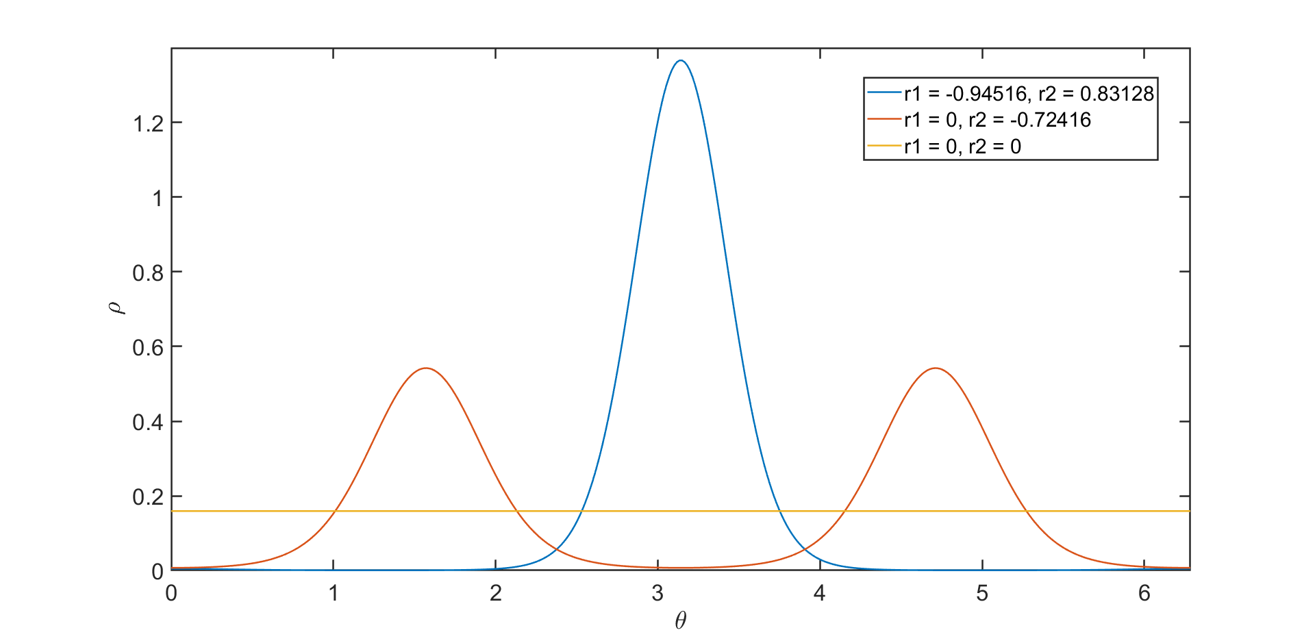
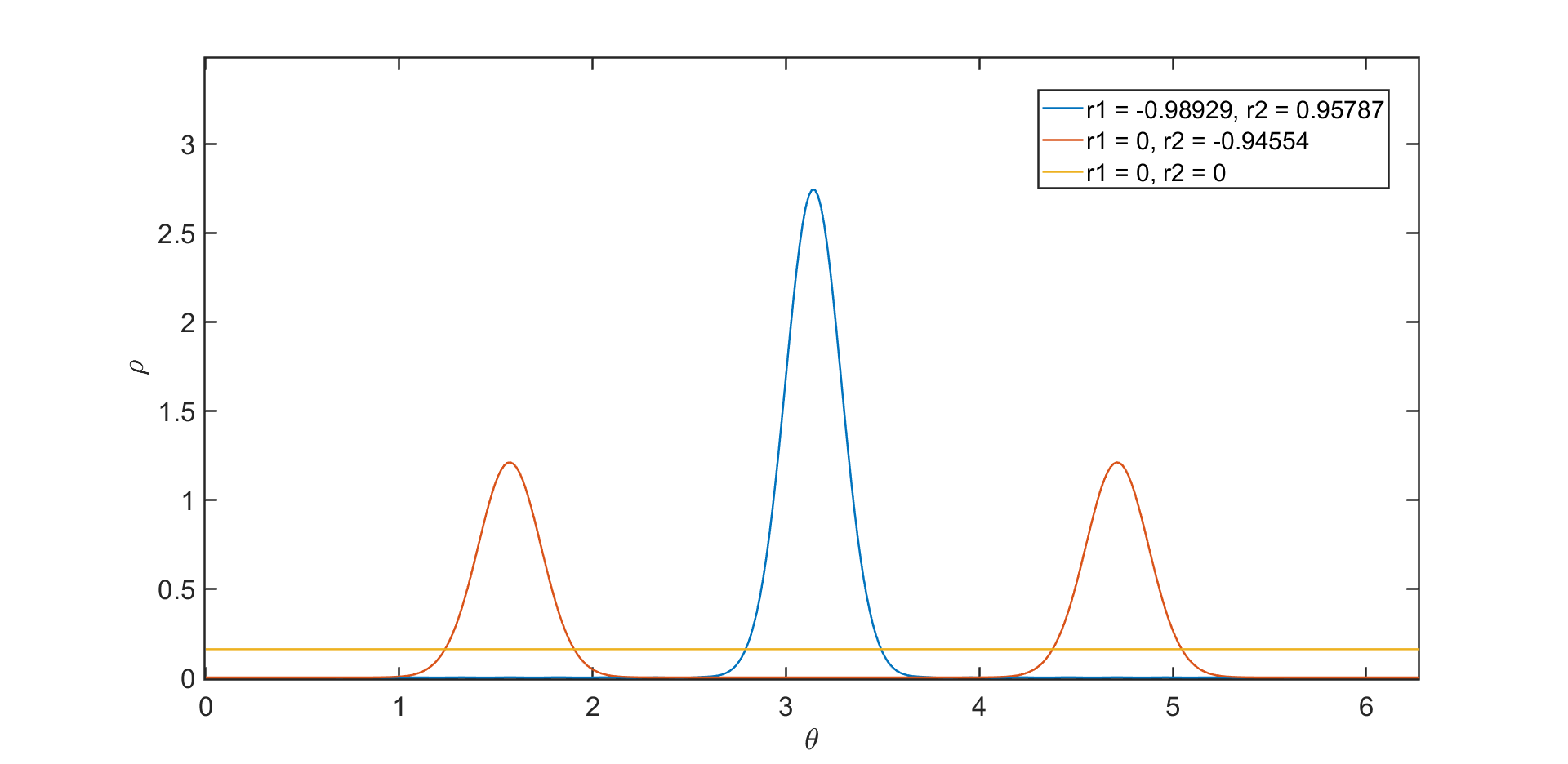
Figure 1: Probability distributions corresponding to the three different solutions for $(r_{1},r_{2})$ for $\beta=3$ (left) and $\beta=10$ (right).

Note that, alongside the uniform distribution, there is a one-peak steady state (as also seen for the Kuramoto model), and we now have a further solution with two peaks, reflecting the multichromatic nature of the interaction potential.

In the following section we aim to address the question of stability of such solutions.

3 Stability Analysis

We perform the stability calculations in two ways. As before, for interaction potentials that are not $H-$stable we expect a critical value of $\beta$ above which the McKean-Vlasov PDE admits stationary solutions other than the uniform state. This critical value is given by $\beta_{c}=\frac{1}{T_{c}}$, where $T_{c}=\min_{1\leq k\leq n}\left\{-\frac{a_{k}}{2}:1\leq k\leq n\right\}$. We will identify this critical temperature in three ways: firstly we analyse the second variation of the free energy, then we perform a linear stability analysis of the PDE, and finally we analyse the problem numerically. These methods will also give us an insight on the stability of the states we find.

3.1 Second variation of the free energy

The first approach we use to perform the linear stability analysis and to identify the continuous phase transition, based on the one used in [10], consists in analysing the eigenvalues of the second variation of the free energy. We first present the calculation in the absence of a confining potential. We recall that the free energy of this system is given by

$$F(\rho)=\frac{1}{2}\int_{0}^{2\pi}\int_{0}^{2\pi}W(x-y)\rho(x)\rho(y)\,\mathrm{d}x\,\mathrm{d}y+\beta^{-1}\int_{0}^{2\pi}\rho(x)\log(\rho(x))\,\mathrm{d}x.$$

Its second variation is

$$\delta^{2}F[\delta\rho,\,\delta\rho]=\frac{1}{2}\int\delta\rho\delta\phi\,\mathrm{d}x+\frac{\beta^{-1}}{2}\int\frac{(\delta\rho)^{2}}{\rho}\,\mathrm{d}x,$$

where $\delta\rho$ is the perturbation and:

$$\delta\phi(x)=\int_{0}^{2\pi}W(x-y)\delta\rho(y)\,\mathrm{d}y.$$

For our interaction potential $W(x)=-\sum_{k=1}^{n}a_{k}\cos(kx)$, this is equal to:

$$\delta^{2}F=(2\pi)^{2}\sum_{j=1}^{\infty}\left(\beta^{-1}+\frac{a_{j}}{2}\right)|\delta\hat{\rho}_{j}|^{2}.$$

We then write:

$$\delta\rho=\frac{\,\mathrm{d}q}{\,\mathrm{d}x},\text{ where }q(x)=\int_{0}^{x}\delta\rho(y,t)\,\mathrm{d}y,$$

to obtain:

$$\delta^{2}F =\frac{1}{2}\int_{0}^{2\pi}\delta\rho\delta\phi\,\mathrm{d}x+\frac{\beta^{-1}}{2}\int_{0}^{2\pi}\frac{(\delta\rho)^{2}}{\rho}\,\mathrm{d}x.$$

This gives, for the first integral:

$$\frac{1}{2}\int_{0}^{2\pi}\delta\rho\delta\phi\,\mathrm{d}x=\frac{1}{2}\int_{0}^{2\pi}\int_{0}^{2\pi}q(x)\frac{\,\mathrm{d}}{\,\mathrm{d}x}\frac{\,\mathrm{d}}{\,\mathrm{d}y}W(x-y)q(y)\,\mathrm{d}x\,\mathrm{d}y,$$

and for the second integral:

$$\frac{\beta^{-1}}{2}\int_{0}^{2\pi}\frac{(\delta\rho)^{2}}{\rho}\,\mathrm{d}x =-\frac{\beta^{-1}}{2}\int_{0}^{2\pi}q(x)\frac{\,\mathrm{d}}{\,\mathrm{d}x}\left(\frac{1}{\rho(x)}\frac{\,\mathrm{d}}{\,\mathrm{d}x}q(x)\right)\,\mathrm{d}x.$$

Therefore, the second variation of the free energy can be written as a quadratic form/integral operator:

$$\delta^{2}F[q,q]=\int_{0}^{2\pi}\int_{0}^{2\pi}K(x,y)q(x)q(y)\,\mathrm{d}x\,\mathrm{d}y,$$

where the kernel is defined as

$$K(x,y)=\frac{1}{2}\sum_{k=1}^{n}k^{2}a_{k}\cos(k(x-y))-\frac{\beta^{-1}}{2}\delta(x-y)\frac{\,\mathrm{d}}{\,\mathrm{d}x}\left(\frac{1}{\rho}\frac{\,\mathrm{d}}{\,\mathrm{d}x}\right).$$

We are therefore led to considering the eigenvalue problem:

$$2\pi\frac{\,\mathrm{d}^{2}q}{\,\mathrm{d}x^{2}}+\beta\int_{0}^{2\pi}q(y)\left(\sum_{k=1}^{n}k^{2}a_{k}\cos(k(x-y))\right)\,\mathrm{d}y=-2\lambda q.$$ (11)

The eigenmodes are $q_{m}=A_{m}\cos(mx)$, $q_{m}=B_{m}\sin(mx)$, where $A_{m},B_{m}\in\mathbb{R}$. It is sufficient to consider the even eigenfunctions. Using trigonometric identities, we can compute the eigenvalues of the integral operator. We first conclude that, for $n<|m|$, we have $\lambda_{m}=\pi m^{2}>0$, so these modes do not induce instability. For $|m|\leq n$, we have

$$\lambda_{m}=-\frac{1}{2}\left(-2\pi m^{2}-\beta m^{2}a_{m}\pi\right)=\pi m^{2}\left(2+\beta a_{m}\right)$$

This is positive for $\beta a_{m}<-2$, so $\beta<-\frac{a_{m}}{2}$. As we are concerned with the first point of linear instability, the critical temperature is $\beta_{c}:=\min_{k}\{-\frac{2}{a_{k}}:1\leq k\leq n\}$, see also [9]. As an example, we note that by setting $a_{1}=-1,a_{k}=0$ for $2\leq n$, we obtain the known result for the Kuramoto model, $\beta_{c}=2$. Similarly, for the interaction potentials $W(x)=-3\cos(x)-\cos(2x)$ or $W(x)=-\cos(x)-\cos(2x)-3\cos(3x)$, the critical temperature is $\beta_{c}=\frac{2}{3}$, as the critical value is not influenced by which Fourier mode has the highest coefficient, but rather by the magnitude of the coefficient itself. Critical temperatures for more examples can be found, together with the corresponding numerical simulations, in Section 5.

Our goal is now to extend this method to study the stability of nonuniform steady states. This extension is not straightforward, and the details will be presented in future work. Here we present only a specific example. We consider $W(x)=-\cos(x)-\frac{1}{2}\cos(2x)$, $V(x)=0$. The nonuniform stationary state is given by $\tilde{\rho}=\frac{1}{Z}\exp\left(\beta\left(-r_{1}\cos(x)-\frac{r_{2}}{2}\cos(2x)\right)\right)$ with $r_{1},r_{2}\neq 0$. The eigenvalue problem for the second variation of the free energy, computed at the nonuniform steady state, becomes:

$$\frac{\,\mathrm{d}}{\,\mathrm{d}x}\left(\frac{1}{\tilde{\rho}}\frac{\,\mathrm{d}q}{\,\mathrm{d}x}\right)-\beta\int_{0}^{2\pi}q(y)(\cos(x-y)+2\cos(2(x-y))\,\mathrm{d}y=-2\lambda q.$$

We need to consider the following operator:

$$\frac{\,\mathrm{d}^{2}q}{\,\mathrm{d}x^{2}}\left(Ze^{\beta f(x)}\right)+\frac{\,\mathrm{d}q}{\,\mathrm{d}x}\left(Z\beta f^{\prime}(x)e^{\beta f(x)}\right)-\beta\int_{0}^{2\pi}q(y)\left(\cos(x-y)+4\cos(2(x-y))\right)\,\mathrm{d}y$$

where $f(x):=-r_{1}\cos(x)-r_{2}\cos(2x)$.

We study the eigenvalue problem numerically for fixed values of $\beta$ and $r_{1}$ and $r_{2}$. Let us first consider the pair $(r_{1},r_{2})$ that appears immediately above the critical temperature, i.e. the pair for which $r_{1},r_{2}\neq 0$, and which corresponds to the one-peak steady state. In this case, we identify a change in the behaviour of the eigenvalues at around $\beta=4.5$. This is the point at which the self consistency equations go from having two solutions to three. For $\beta<4.5$, all eigenvalues are negative, while at $\beta=4.5$ we start seeing some positive eigenvalues as well, indicating that the stability of this steady state changes as the third stationary distribution appears. On the other hand, the operator corresponding to the multipeak solution (i.e. to the pair of coefficients $(0,r_{2})$) seems to have a mix of positive and negative eigenvalues for any value of $\beta$.

3.2 Linearisation of the Fokker-Planck equation

We can calculate the value of the critical temperature also by looking at the Fourier modes of the linearisation of the Fokker-Plank PDE:

$$\frac{\partial\rho}{\partial t}(t,x)=\frac{\partial}{\partial x}\left[\left(\int\rho(t,x-y)W^{\prime}(y)\,\mathrm{d}y\right)\rho(t,x)\right]+\beta^{-1}\frac{\partial^{2}\rho}{\partial x^{2}}(t,x).$$

Following the method in [19], we decompose $\rho=\rho_{0}+\rho_{1}=\frac{1}{2\pi}+\rho_{1}$, where $\rho_{1}$ is a small perturbation of $\rho$ so that $O(\rho_{1}^{2})$ is negligible. In the Fourier domain the PDE becomes:

$$\frac{\partial\hat{\rho}_{1}(t,j)}{\partial t}=\left[i\rho_{0}j\int e^{-ijy}W^{\prime}(y)\,\mathrm{d}y-\beta^{-1}j^{2}\right]\hat{\rho_{1}}(t,j),$$

where $\hat{\rho}_{1}(j)$ is the $j$-th Fourier coefficient of $\rho_{1}$. Therefore, the Fourier modes have growth rates:

$$\gamma_{j}=\text{Re}\left[i\rho_{0}j\int e^{-ijy}W^{\prime}(y)\,\mathrm{d}y-\beta^{-1}j^{2}\right]=\rho_{0}j\int\sin(jy)W^{\prime}(y)\,\mathrm{d}y-\beta^{-1}j^{2}.$$

Substituting $W^{\prime}(x)=-\sum_{k=1}^{n}ka_{k}\sin(kx)$, our problem reduces to studying the sign of:

$$\gamma_{j}=-\frac{j}{2\pi}\int_{0}^{2\pi}\sin(jy)\sum_{k=1}^{n}ka_{k}\sin(ky)\,\mathrm{d}y-\beta^{-1}j^{2},$$

as $\beta$ varies. For $j>n$, the integral term above is equal to $0$. Hence:

$$\gamma_{j}=-\beta^{-1}j^{2}.$$

As this is always negative, these modes do not induce instability. For $j\leq n$:

$$\gamma_{j}=-\frac{1}{2\pi}\int_{0}^{2\pi}\sin(jy)\sum_{k=1}^{n}ka_{k}\sin(ky)\,\mathrm{d}y-\beta^{-1}j=-\frac{ja_{j}}{2}-\beta^{-1}j.$$

This is positive for $2\beta^{-1}<-a_{j}$, i.e. for $\beta>-\frac{2}{a_{j}}$, as expected from the calculations in the previous sections.

4 Perturbation analysis

Our next goal is to study the stability of non-uniform stationary states close to the critical interaction strength. One approach would be to linearize the McKean-Vlasov operator

$$\mathcal{L}\rho=\beta^{-1}\partial_{x}^{2}\rho+\partial_{x}\left(\partial_{x}V\rho\right)+\theta\partial_{x}\left((\partial_{x}W\star\rho)\rho\right)$$ (12)

around the (non-uniform) stationary state $\rho_{\infty}$, the solution of the stationary McKean-Vlasov PDE

$$\beta^{-1}\partial_{x}^{2}\rho_{\infty}+\partial_{x}\left(\partial_{x}V\rho_{\infty}\right)+\theta\partial_{x}\left((\partial_{x}W\star\rho_{\infty})\rho_{\infty}\right)=0,$$ (13)

on $[0,2\pi]$ with periodic boundary conditions, and where $\theta$ denotes the interaction strength. The linearized operator is

$$\mathcal{L}_{\rho_{\infty}}\rho = \beta^{-1}\partial_{x}^{2}\rho+\partial_{x}(\partial_{x}V\rho)+\theta\partial_{x}((\partial_{x}W\star\rho_{\infty})\rho)+\theta\partial_{x}((\partial_{x}W\star\rho)\rho_{\infty})$$ (14)

$$=: \beta^{-1}\partial_{x}^{2}\rho+\partial_{x}(\mathcal{U}_{\theta}\rho)+\int\kappa_{\theta}(x,y)\rho(y)\,dy.$$

In writing the above, we have introduced the effective potential $\mathcal{U}_{\theta}$. This is an integro-differential Fokker–Planck operator. Via the standard ground state transformation we can map it to a nonlocal Schrödinger operator [31][Sec. 4.9], of the form considered in [12, 13], albeit with different boundary conditions. The spectral properties of (14) will be studied elsewhere.

Instead of considering (14), we follow [5][Sec. 2.5] (Eqn (2.57)) and perform the ground state transformation before the linearization to map the McKean-Vlasov operator to a nonlinear and nonlocal Schrödinger operator. The nonlinearity and nonlocality enter through the dependence on the Fourier modes of the stationary states that satisfy the self-consistency equations. See also [34, Sec. 3].

The Schrödinger operator for the noisy Kuramoto model is:

$$Hf=f^{\prime\prime}-\frac{1}{2}\left(\frac{\beta^{2}}{2}r^{2}\sin^{2}(x)+\beta r\cos(x)\right)f.$$

We consider the self-consistency equation (6) close to the critical inverse temperature $\beta=2(1+\varepsilon$), for a small $\varepsilon>0$. For $\beta$ close to $2$, we use the approximation $r(\beta)\approx\sqrt{1-\frac{2}{\beta}}$ [5][Sec. 2.5]. Substituting these values of $r$ and $\beta$ in the expression for $H$:

$$Hf =f^{\prime\prime}-\left(\varepsilon\sin^{2}(x)+\varepsilon^{2}\sin^{2}(x)+\sqrt{\varepsilon(1+\varepsilon)}\cos(x)\right)f.$$

Now, using the Taylor expansion for $\sqrt{1+\varepsilon}$, we have $\sqrt{\varepsilon(1+\varepsilon)}=\sqrt{\varepsilon}+O(\varepsilon\sqrt{\varepsilon})$. We set $\delta=\sqrt{\varepsilon}$ and can then rewrite the equation for $H$ as:

$$Hf=f^{\prime\prime}-\delta\cos(x)f-\delta^{2}\sin^{2}(x)f+O(\delta^{3})=:H_{0}+\delta H_{1}+\delta^{2}H_{2}+O(\delta^{3}).$$

Therefore, we can consider $H$ as a small perturbation of the operator $H_{0}f=f^{\prime\prime}$. Our goal is to calculate the eigenvalues of $H$ perturbatively for small $\delta$. We consider the eigenvalue problem

$$H\psi=E\psi.$$ (15)

We expand $E$ and $\psi$ in power series in $\delta$:

$$\psi=\psi_{0}+\delta\psi_{1}+\delta^{2}\psi_{2}+\ldots$$

$$E=E_{0}+\delta E_{1}+\delta^{2}E_{2}+\ldots$$

We substitute these expansions into (15) to obtain the following sequence of equations.

Order $O(1)$: $H_{0}\psi_{0}=E_{0}\psi_{0}$.

The eigenvalues of $H_{0}$ are given by $E^{(m)}=-m^{2}$ for $m\in\mathbb{N}$, and the corresponding eigenfunctions are $\psi^{(m)}(x)=A_{m}\cos(mx)+B_{m}\sin(mx)$, $A_{m},B_{m}\in\mathbb{R}$. Due to the symmetry of the interaction potential, we will only consider even eigenfunctions, i.e. $B_{m}=0$ for all $m\in\mathbb{N}$. We take $A_{m}=\frac{1}{\sqrt{\pi}}$ so that $\langle\psi_{0},\psi_{0}\rangle=1$.

Order $O(\delta)$: $H_{0}\psi_{1}+H_{1}\psi_{0}=E_{0}\psi_{1}+E_{1}\psi_{0}$.

We take the inner product of both sides with $\psi_{0}$ to obtain:

$$\langle\psi_{0},H_{0}\psi_{1}\rangle+\langle\psi_{0},H_{1}\psi_{0}\rangle=E_{0}\langle\psi_{0},\psi_{1}\rangle+E_{1}\langle\psi_{0},\psi_{0}\rangle.$$

Since $H_{0}$ is self-adjoint in $L^{2}(0,2\pi)$, we obtain:

$$E_{1}=\frac{\langle\psi_{0},H_{1}\psi_{0}\rangle}{\langle\psi_{0},\psi_{0}\rangle}=0,$$

Order $O(\delta^{2})$: $H_{0}\psi_{2}+H_{1}\psi_{1}+H_{2}\psi_{0}=E_{0}\psi_{2}+E_{1}\psi_{1}+E_{2}\psi_{0}=E_{0}\psi_{2}+E_{2}\psi_{0}$. We take again the inner product with $\psi_{0}$ and use the self-adjointness of $H_{0}$ to obtain:

$$E_{2}=\frac{\langle\psi_{0},H_{1}\psi_{1}+H_{2}\psi_{0}\rangle}{\langle\psi_{0},\psi_{0}\rangle}=\langle\psi_{0},H_{1}\psi_{1}+H_{2}\psi_{0}\rangle.$$

We now calculate $\psi_{1}$. It satisfies the equation

$$H_{0}\psi_{1}+H_{1}\psi_{0}=E_{0}\psi_{1},$$

which takes the form

$$\psi_{1}^{\prime\prime}+m^{2}\psi_{1}=\frac{1}{\sqrt{\pi}}\cos(x)\cos(mx),$$

in $(0,2\pi)$ with periodic boundary conditions. This is a second order inhomogeneous ODE; its solution is:

$$\psi_{1}(x) = \frac{1}{(4m^{2}-1)\sqrt{\pi}}\Big{(}2m\sin(x)\sin(mx)+\cos(x)\cos(mx)\Big{)}+C_{2}\sin(mx)+C_{1}\cos(mx),$$

for $C_{1},C_{2}\in\mathbb{R}$.

We can now calculate $\langle\psi_{0},H_{1}\psi_{1}\rangle$:

$$\langle\psi_{0},H_{1}\psi_{1}\rangle=\begin{cases}-\frac{5}{12}\text{ if }m=1\\ -\frac{1}{2(4m^{2}-1)}\text{ if }m\neq 1.\end{cases}$$

Similarly, we have:

$$\langle\psi_{0},H_{2}\psi_{0}\rangle=\begin{cases}-\frac{1}{2}\text{ if }m\neq 1\\ -\frac{1}{4}\text{ if }m=1.\end{cases}$$

We conclude that for $m=1$ the second order perturbation is $E_{2}=-\frac{2}{3}$, and for $m\neq 1$:

$$E_{2}=-\frac{1}{2(4m^{2}-1)}-\frac{1}{2},$$

The eigenvalue of the perturbed operator $H$ is hence given by: $E=E_{0}+\delta E_{1}+\delta^{2}E_{2}=-m^{2}+\delta^{2}E_{2}$.

We are primarily interested in the first nonzero eigenvalue. We plot the asymptotic formula $E=-1-\frac{2}{3}\delta^{2}$ versus the numerically obtained ones. The latter are obtained by using Matlab’s eig function on the operator $Hf=f^{\prime\prime}-\delta\cos(x)f-\delta^{2}\sin^{2}(x)f$

Figure 2: First eigenvalue as a function of $\delta$, $W(x)=-\cos(x)$.

4.1 A higher order harmonic potential

We now consider the interaction potential $W(x)=-\cos(nx)$. The Schrödinger operator becomes:

$$Hf=f^{\prime\prime}-\frac{n^{2}}{2}\left(\frac{\beta^{2}}{2}r^{2}\sin^{2}(nx)+\beta r\cos(nx)\right)f(x).$$

Writing $\beta=2(1+\varepsilon)$ and using the same expansion as before, we obtain:

$$Hf=f^{\prime\prime}-\delta n^{2}\cos(nx)f(x)-\delta^{2}n^{2}\sin^{2}(nx)f(x)+O(\delta^{3})=:H_{0}+\delta H_{1}+\delta^{2}H_{2}+O(\delta^{3}).$$

We note that we can indeed use the same expansion for $r$ as before, as this comes from using the Taylor expansion on $\exp(\beta r\cos(kx))$ and all terms involving the $\cos(kx)$ terms simplify. More precisely, we now have:

$$r=\frac{\int_{0}^{2\pi}\cos(nx)\exp(\beta r\cos(nx))\,\mathrm{d}x}{\int_{0}^{2\pi}\exp(\beta r\cos(nx))\,\mathrm{d}x}.$$

Approximating $e^{x}\approx 1+x+\frac{x^{2}}{2}$:

$$r =\frac{\int_{0}^{2\pi}\cos(nx)+\beta r\cos(nx)^{2}+\frac{\beta^{2}}{2}r^{2}\cos(nx)^{3}\,\mathrm{d}x}{\int_{0}^{2\pi}1+\beta r\cos(nx)+\frac{\beta^{2}}{2}r^{2}\cos(nx)^{2}\,\mathrm{d}x}=\frac{\beta r\pi}{2\pi+\frac{\beta^{2}}{2}r^{2}\pi}.$$

Substituting $\beta=2(1+\varepsilon)$, we deduce that

$$r=\frac{\sqrt{\varepsilon}}{1+\varepsilon}.$$

We study again the equations corresponding to different orders of $\delta=\sqrt{\varepsilon}$.

Order $O(1)$: $H_{0}\psi_{0}=E_{0}\psi_{0}$. As before, this is just the eigenvalue equation for the unperturbed operator $H_{0}f=f^{\prime\prime}$. Therefore, $\psi_{0}(x)=-\frac{1}{\sqrt{\pi}}\cos(mx)$ for $m\in\mathbb{N}$.

Order $O(\delta)$: $H_{0}\psi_{1}+H_{1}\psi_{0}=E_{0}\psi_{1}+E_{1}\psi_{0}$. Using the same reasoning as with the previous case, we obtain:

$$E_{1}=\langle\psi_{0},H_{1}\psi_{0}\rangle=\begin{cases}0&\text{ if }n\neq 2m\\ -\frac{n^{2}}{2}&\text{ if }n=2m.\end{cases}$$

Therefore, when $n$ is even, we now have a non-zero first order perturbation; the corresponding eigenvalues of $H$ are:

$$E=-\frac{n^{2}}{2}\left(\frac{1}{2}+\delta\right).$$

Order $O(\delta^{2})$: $H_{0}\psi_{2}+H_{1}\psi_{1}+H_{2}\psi_{0}=E_{0}\psi_{2}+E_{1}\psi_{1}+E_{2}\psi_{0}$.

As before:

$$E_{2}=\langle\psi_{0},H_{1}\psi_{1}+H_{2}\psi_{0}\rangle$$

We only look at the second perturbation in the case where $E_{1}=0$, i.e. when $n\neq 2m$. Performing the same calculations as in the previous subsection, we obtain that for $n\neq m$:

$$E_{2}=\frac{n^{2}}{(n^{2}-4m^{2})}\left(\frac{n^{2}}{2}\right)-\frac{n^{2}}{2},$$

while for $n=m$:

$$E_{2} =-\frac{5n^{2}}{12}-\frac{n^{2}}{4}=\frac{2n^{2}}{3}.$$

Therefore, we obtain the following eigenvalues for $H$:

• For $n\in\mathbb{N}$ even, $E_{n}=-\frac{n^{2}}{2}\left(\frac{1}{2}+\delta\right)$;

• For $n,m\in\mathbb{N}$, $m\neq\frac{n}{2}$, $E_{n}=-m^{2}+\delta^{2}\left(\frac{n^{2}}{(n^{2}-4m^{2})}\left(\frac{n^{2}}{2}\right)-\frac{n^{2}}{2}\right)$;

• For $n\in\mathbb{N}$, $E_{n}=-n^{2}-\delta^{2}\left(\frac{n^{2}}{6}\right)$.

Table 1: Eigenvalues for $W(x)=-\cos(2x)$, $\delta=0.1$.

m	Perturbation eigenvalue	Numerical eigenvalue
1	-1.2	-1.2154
2	-4.0267	-4.0267
3	-9.0225	-9.0221
4	-16.0213	-16.0213

Table 2: Eigenvalues for $W(x)=-\cos(3x)$, $\delta=0.1$.

m	Perturbation eigenvalue	Numerical eigenvalue
1	-0.964	-0.9653
2	-4.1029	-4.1015
3	-9.06	-9.0600
4	-16.0524	-16.0524

Table 3: Eigenvalues for $W(x)=-\cos(4x)$, $\delta=0.1$.

m	Perturbation eigenvalue	Numerical eigenvalue
1	-0.9733	-0.9739
2	-4.8	-4.8615
3	-9.144	-9.1434
4	-16.067	-16.067

4.2 Multichromatic potentials

We now consider $W(x)=-\cos(x)-\frac{1}{2}\cos(2x)$. We recall that now the stationary distribution is given by:

$$\rho_{\infty}(x)=\frac{\exp(\beta(r_{1}\cos(x)+\frac{r_{2}}{2}\cos(2x)))}{\int_{0}^{2\pi}\exp(\beta(r_{1}\cos(x)+\frac{r_{2}}{2}\cos(2x)))\,\mathrm{d}x}$$ (16)

with $r_{1}$ and $r_{2}$ satisfying the self-consistency equations:

$$r_{1}=\frac{\int_{0}^{2\pi}\cos(x)\exp(\beta(r_{1}\cos(x)+\frac{r_{2}}{2}\cos(2x)))\,\mathrm{d}x}{\int_{0}^{2\pi}\exp(\beta(r_{1}\cos(x)+\frac{r_{2}}{2}\cos(2x)))\,\mathrm{d}x}$$ (17)

and

$$r_{2}=\frac{\int_{0}^{2\pi}\cos(2x)\exp(\beta(r_{1}\cos(x)+\frac{r_{2}}{2}\cos(2x)))\,\mathrm{d}x}{\int_{0}^{2\pi}\exp(\beta(r_{1}\cos(x)+\frac{r_{2}}{2}\cos(2x)))\,\mathrm{d}x}$$ (18)

We need to find approximations for $r_{1}$ and $r_{2}$ near the critical value of $\beta$. Using that $\exp(x)\sim 1+x+\frac{x^{2}}{2}$ in equations (17)-(18), we obtain that, close to $\beta=2$, $r_{2}^{2}(\beta)$ behaves linearly, and that

$$r_{1}=\sqrt{r_{2}\left(r_{2}+\frac{2}{\beta}\right)}.$$ (19)

To obtain an explicit expression for $r_{2}(\beta)$ we use a basic fitting algorithm to obtain that the best approximation is given by

$$r_{2}(\beta)=\sqrt{\frac{3}{2}-\frac{3}{\beta}}.$$

Substituting this in (19), we obtain the corresponding approximating function for $r_{1}$:

$$r_{1}(\beta)=\sqrt{\frac{3}{2}-\frac{3}{\beta}+\frac{2}{\beta}\sqrt{\frac{3}{2}-\frac{3}{\beta}}}$$

We now use these approximations to study the Schrödinger operator for $W=-\cos(x)-\frac{1}{2}\cos(2x)$. With $\rho_{\infty}$ as in (16), we have that:

$$U(x):=\frac{\beta}{2}W*\rho_{\infty}(x)=-\frac{\beta}{2}r_{1}\cos(x)-\frac{\beta}{4}r_{2}\cos(2x)$$

Therefore:

$$\mathcal{L}f=f^{\prime\prime}-\left(\frac{(U^{\prime})^{2}}{4}+\frac{U^{\prime\prime}}{2}\right)f$$

$$=f^{\prime\prime}-\left(\frac{\beta^{2}}{4}(r_{1}\sin(x)+r_{2}\sin(2x))^{2}+\frac{\beta}{2}(r_{1}\cos(x)+2r_{2}\cos(2x))\right)f$$

We now substitute $\beta=2(1+\varepsilon)$, $\eta={\varepsilon}^{1/4}$, use the above expressions for $r_{1}(\beta),r_{2}(\beta)$ and ignore terms of order higher than $O(\eta^{3})$. After long calculations, we obtain the following expression for the perturbed operator:

$$Hf :=f^{\prime\prime}-\left(\sqrt{\frac{3}{2}}\eta^{2}\sin^{2}(x)+\left(\frac{3}{2}\right)^{1/4}\eta\cos(x)+2\sqrt{\frac{3}{2}}\eta^{2}\cos(2x)\right)f$$

$$=:H_{0}+\eta H_{1}+\eta^{2}H_{2},$$

where

$$H_{0}f=f^{\prime\prime};$$

$$H_{1}f=-\left(\frac{3}{2}\right)^{1/4}\cos(x)f(x);$$

$$H_{2}f=-\sqrt{\frac{3}{2}}\left(\sin^{2}(x)+2\cos(2x)\right)f(x)=-\frac{1}{2}\sqrt{\frac{3}{2}}(1+3\cos(2x))f(x).$$

We do the usual perturbation argument to find the eigenvalues $E$ and eigenfunctions $\psi$ solving $H\psi=E\psi$. We solve the equation order by order.

Order $O(1)$: $H_{0}\psi_{0}=E_{0}\psi_{0}$.

As usual, this gives us $\psi_{0}=\frac{1}{\sqrt{\pi}}\cos(nx)$, $E_{0}=-n^{2}$.

Order $O(\eta)$: $H_{0}\psi_{1}+H_{1}\psi_{0}=E_{0}\psi_{1}+E_{1}\psi_{0}$. Performing the same steps as before gives us $E_{1}=0$ again.

Order $O(\eta^{2})$: $H_{0}\psi_{2}+H_{1}\psi_{1}+H_{2}\psi_{0}=E_{0}\psi_{2}+E_{1}\psi_{1}+E_{2}\psi_{0}=E_{0}\psi_{2}+E_{2}\psi_{0}$. We again take the inner product with $\psi_{0}$ and use that $H_{0}$ is Hermitian to obtain:

$$E_{2}=\langle\psi_{0},H_{1}\psi_{1}+H_{2}\psi_{0}\rangle$$

Solving similar equations as in the previous subsections we have, for $n=1$:

$$E_{2}=-\frac{(36)^{1/4}}{12}-\frac{3}{2}\sqrt{\frac{3}{2}}$$

and for $n\neq 1$:

$$E_{2}=-\frac{1}{2}\sqrt{\frac{3}{2}}\left(\frac{1}{4n^{2}-1}+1\right)$$

Therefore, the eigenvalues of $H$ are $E=-1-\eta^{2}\left(\frac{(36)^{1/4}}{12}+\frac{3}{2}\sqrt{\frac{3}{2}}\right)$ and, for $n\neq 1$:

$$E=-n^{2}-\eta^{2}\frac{1}{2}\sqrt{\frac{3}{2}}\left(\frac{1}{4n^{2}-1}+1\right)$$

Fixing $\eta$ (for example, $\eta=0.5$) and calculating a few values, we can see that they are in very good agreement with the eigenvalues found numerically by MATLAB. As before, we provide a plot to illustrate the behaviour of the first eigenvalue as $\eta$ varies.

Figure 3: First eigenvalue as a function of $\eta$, $W(x)=-\cos(x)-\frac{1}{2}\cos(2x)$.

5 Numerical experiments

In this section we consider both steady states and the dynamics of the Fokker-Planck equation (1) by solving it numerically using pseudospectral methods  [7, 28, 21]. Furthermore, we compare the solution of the PDE to results obtained from Monte-Carlo simulations using the Euler-Maruyama method [23].

5.1 Steady states and intermediate dynamics

As described in Section 2, we expect there to be a qualitative change in the nature of the steady-state solution of the PDE (1) at $\beta_{c}=T_{c}^{-1}$. Due to the gradient structure of the PDE, (numerical approximations to the) steady states can be determined either by solving the PDE directly over a long time interval, or by solving the self-consistency equation (4) iteratively, for example via Picard iteration. A key difference here is that iterative approaches can converge to unstable steady states, whereas the PDE method always approaches a stable steady state. This motivates our choice in this section to use the long time PDE solutions.

In order to focus on the effects of the choice of the interaction parameters on the dynamics, in this section we consider dynamics with no external potential. We will reintroduce the external potential in the following section when comparing against stochastic dynamics.

We reiterate from above that for for $\beta<\beta_{c}$, we expect the uniform state to be stable, corresponding to the long time solution of the PDE being $\rho_{\infty}=1/(2\pi)$. In contrast, for $\beta>\beta_{c}$, we expect to observe the other, peaked solutions. Furthermore, as $\beta$ grows larger, we expect the steady state to be more strongly peaked.

In Figures 4–7 we show ‘intermediate’ and ‘long’ time dynamics of the PDE for various interactions, $W$, and a range of $\beta$. The particular choices of $W$ are somewhat arbitrary; we have chosen interactions with $n=2$ and $n=3$ coefficients, with the values chosen to result in a range of different dynamics.

We start with an initial condition that is a small perturbation of the uniform state - $\rho_{0}(x)=\frac{1}{2\pi}+0.01\sin\left(x-\frac{\pi}{2}\right)$. We note that the particular form of the initial condition dictates the position of the peak in the steady state; we have chosen it such that the peak is located at $\theta=\pi$ for clarity. Due to the translational invariance of the problem, this perturbation can, in principle, be chosen to control the position of the peak(s); we will make use of this in the following section when comparing to the SDE dynamics. One may think that, in parameter regimes where the uniform state is unstable, a deliberate perturbation is not necessary to see dynamics, as this should be produced by the accumulation of numerical errors. However, due to the very high accuracy of the chosen numerical schemes we find that it is necessary to deliberately perturb the uniform state in order to induce dynamics in reasonable computational times.

As can be seen in the figures, for $\beta<\beta_{c}$, the long time solution is indeed the numerical steady state. As expected, for $\beta>\beta_{c}$ we see a more interesting range of long time solutions, which (for the examples below) have a single peak. Note that for $\beta$ close to $\beta_{c}$ the convergence to equilibrium can be very slow; this is demonstrated in the right hand plots of Figures 6 and 7 where the solutions for $\beta$ close to $\beta_{c}$ have not yet converged to the final steady state. This effect is due to the exponential slowing down of the dynamics near the critical value of $\beta$.

Considering now the ‘intermediate’ dynamics in the left hand plots of Figures 6 and 7, we note that there are transient regimes where where the number of peaks is the value of $k$ corresponding to the largest $|a_{k}|$. However, these states appear to be unstable as the long time dynamics results in a single peak. The instability of multi-peak steady states was also observed in [33], [20].

Looking at the dynamics in a bit more detail, we see that for the interactions in Figures 4 and 5, the largest (in magnitude) coefficient is $a_{1}$, which corresponds to a single Fourier mode. As expected, this leads to relatively simple dynamics in which the solution quickly converges to a single peak. As shown in Figure 5 adding a third non-zero coefficient does not change the critical value $\beta_{c}$, nor the qualitative nature of the solution. However, it does affect the quantitative dynamics, for example by decreasing the width of the final solutions for fixed $\beta$. There is also a more obvious three-peaked state during the dynamics for $\beta=2$, although it is possible that this arises at a different time for the dynamics in Figure 4.

In Figures 6 and 7 we consider interactions where the largest magnitude coefficient corresponds to a higher Fourier mode. In these cases, we clearly see the transient states which have a number of peaks corresponding to the Fourier mode with the coefficient with the largest magnitude. However, the steady state solution is dominated by the lowest non-zero Fourier mode, which in the cases shown here results in a single peak.

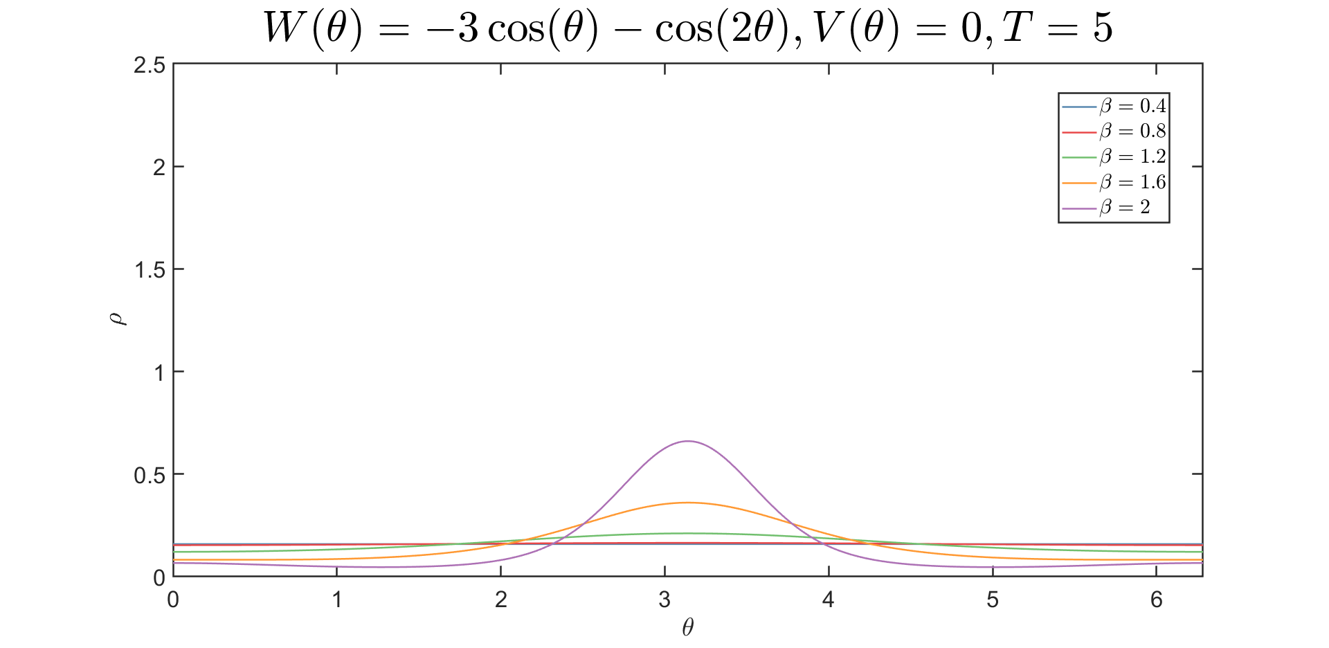
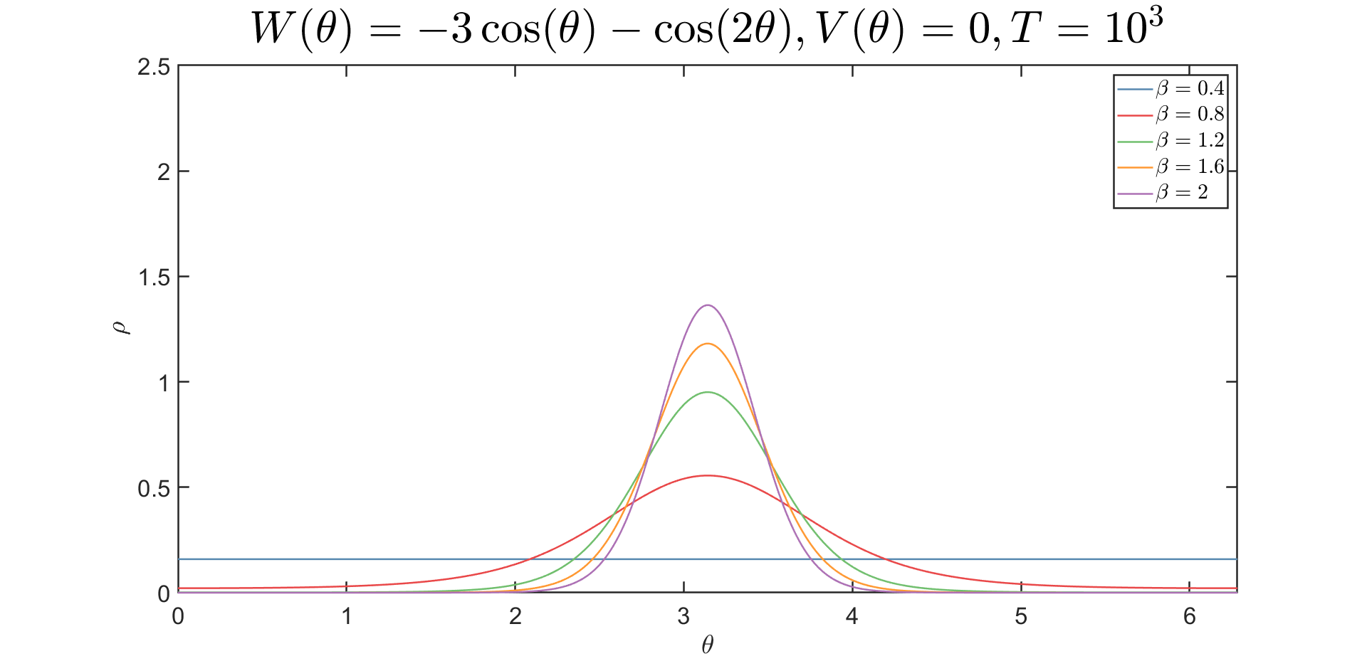
Figure 4: PDE dynamics for different values of $\beta$ for the interacting potential $W(\theta)=-3\cos(\theta)-\cos(2\theta),V(\theta)=0$ for times $T=5$ (left) and $T=10^{3}$ (right). The critical temperature is $\beta_{c}=\frac{2}{3}$.

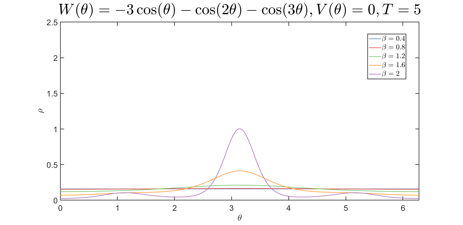
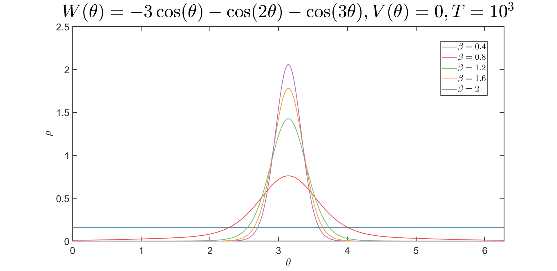
Figure 5: PDE dynamics for different values of $\beta$ for the interacting potential $W(\theta)=-3\cos(\theta)-\cos(2\theta)-\cos(3\theta),V(\theta)=0$ for times $T=5$ (left) and $T=10^{3}$ (right). The critical temperature is $\beta_{c}=\frac{2}{3}$.

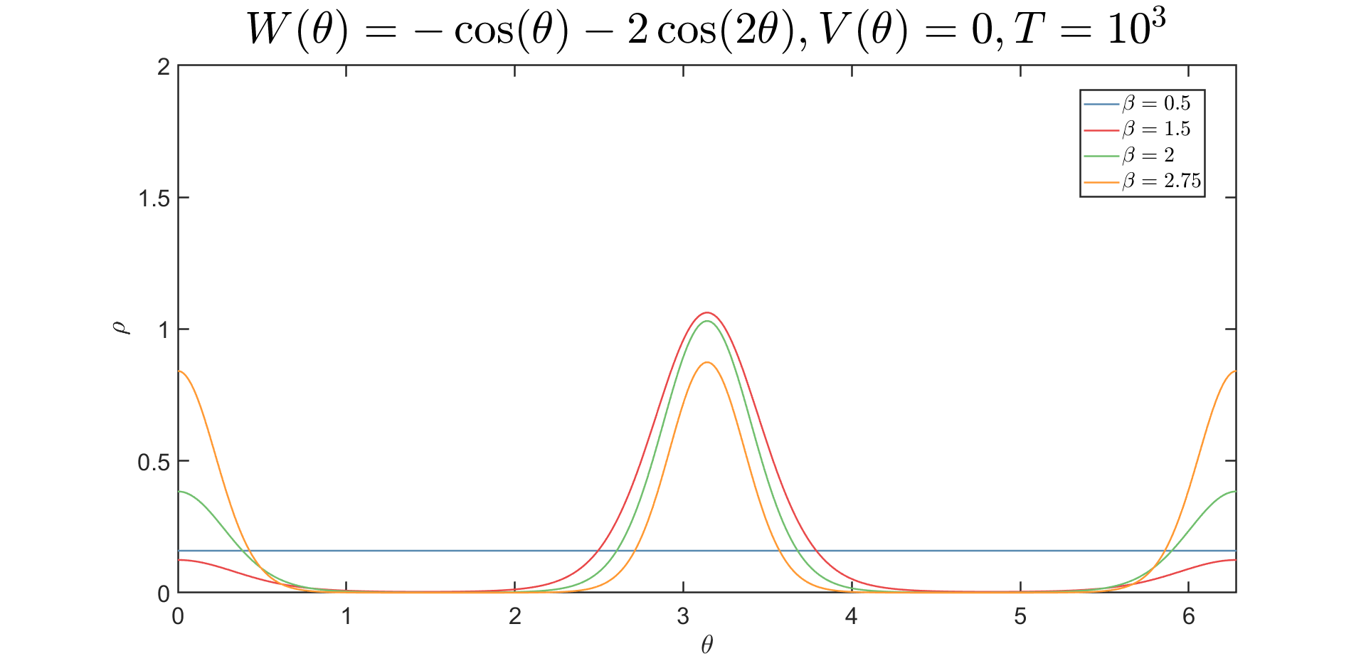
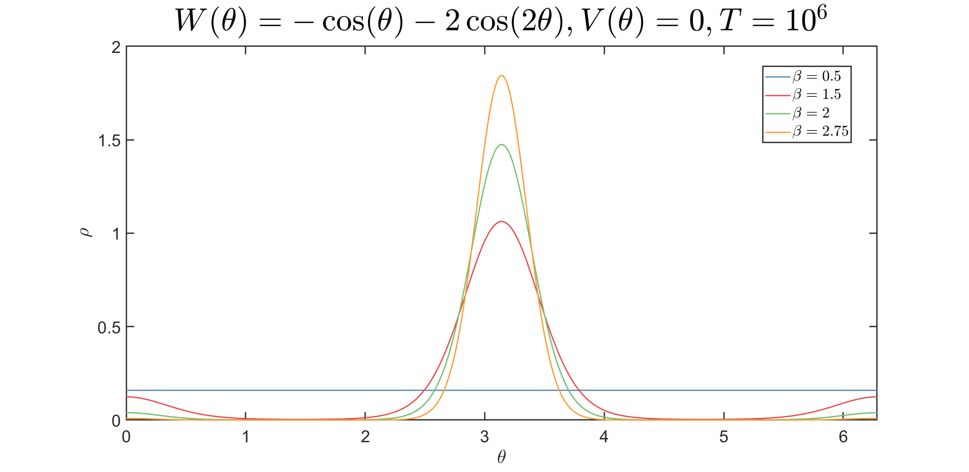
Figure 6: PDE dynamics for different values of $\beta$ for the interacting potential $W(x)=-\cos(x)-2\cos(2x),V(x)=0$, for times $T=10^{3}$ (left) and $T=10^{6}$ (right). The critical temperature is $\beta_{c}=1$.

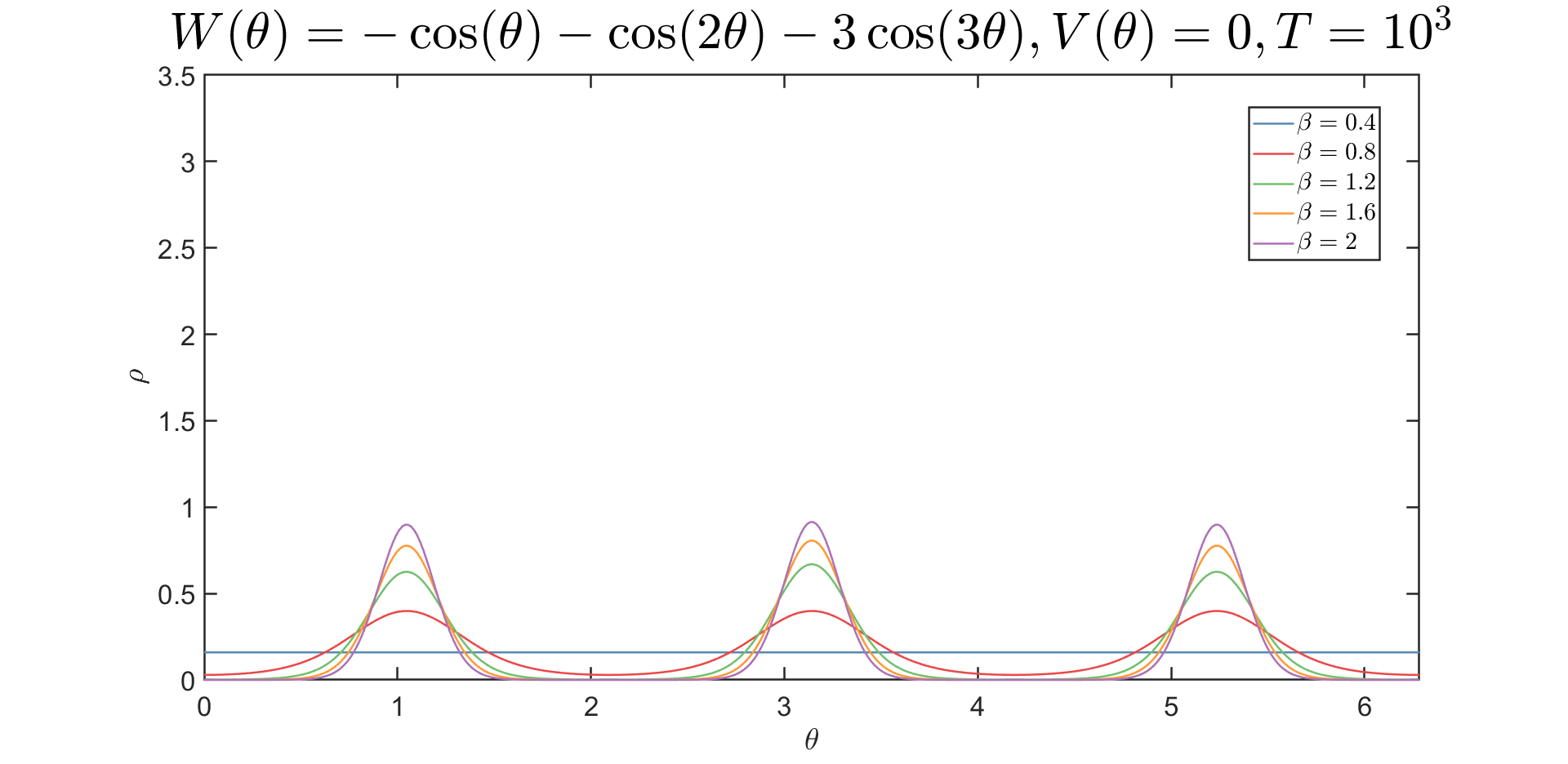
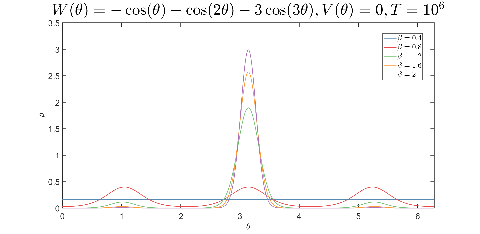
Figure 7: PDE dynamics for different values of $\beta$ for the interacting potential $W(x)=-\cos(x)-\cos(2x)-3\cos(3x),V(x)=0$, for times $T=10^{3}$ (left) and $T=10^{6}$ (right). The critical temperature is $\beta_{c}=\frac{2}{3}$.

Figures 4-7 only show stable steady states with one single peak. It is possible to construct models with stable multipeak stationary distributions by simply rescaling the domain of the interaction potential, i.e. by considering potentials with higher harmonics and with a zero first Fourier mode. For example, the interaction potential $W(x)=-\cos(2x)$ will have a two-peak stable steady state.

5.2 Comparison with Monte Carlo Simulations

In this section we compare the dynamics of the PDE, (1), with those of the underlying interacting particle SDE, (5). The aim here is twofold: we will (i) demonstrate the effects of translational invariance on the results of stochastic sampling, and (ii) compare the PDE and SDE dynamics directly for a single initial condition with a large number of particles; this is a numerical demonstration of the mean-field limiting dynamics agreeing.

We will also investigate systems which have a non-zero confining potential. For a non-trivial potential, this breaks the translational invariance and allows us to demonstrate very good agreement between the two solutions by performing multiple runs of the stochastic dynamics and averaging. This is computationally much cheaper than performing a single run with a larger number of particles: For $N$ particles and $R$ runs, the computational cost scales approximately as $N^{2}R$ (where the $N^{2}$ scaling results from having to compute the interaction potential), so increasing the number of runs is much cheaper than increasing the number of particles.

To numerically solve the SDE  (5), we use the Euler-Maruyama method [23] and compare our findings with the results obtained from the PDE solver. Unless otherwise stated, in all the simulations we use 500 particles, and a timestep of $0.01$. The initial condition is generated by sampling from the same initial condition $\rho_{0}$ as for the PDE given in Section 5.1 using Monte-Carlo slice sampling [27].

We first consider the interaction potential $W(x)=-\cos(x)-\frac{1}{2}\cos(2x)$, with no confining potential, an interaction strength $K=1$, and inverse temperature $\beta=3$. We run the dynamics up to a final time $T=200$.

As mentioned, in the absence of a confining potential, the problem is translationally invariant. This means, in particular, that above the phase transition we have infinitely many stationary states parameterized by an angle $\theta\in[0,2\pi]$ [5]. Consequently, when performing particle simulations, if we average over many realizations of the noise, we obtain (approximately) the uniform distribution; see the left plot in Figure 8. On the other hand, if we perform a single simulation, with a sufficiently large number of particles, then the results of the stochastic simulations are in good agreement with the results of the PDE, up to a translation in space; see the right plot in Figure 8. Note that, in order to more clearly demonstrate the agreement, we have adjusted the PDE initial condition through a translational shift so that the positions of the peaks (approximately) align. This gives exactly the same result as simply re-plotting the PDE (or SDE) solution on a translated axis.

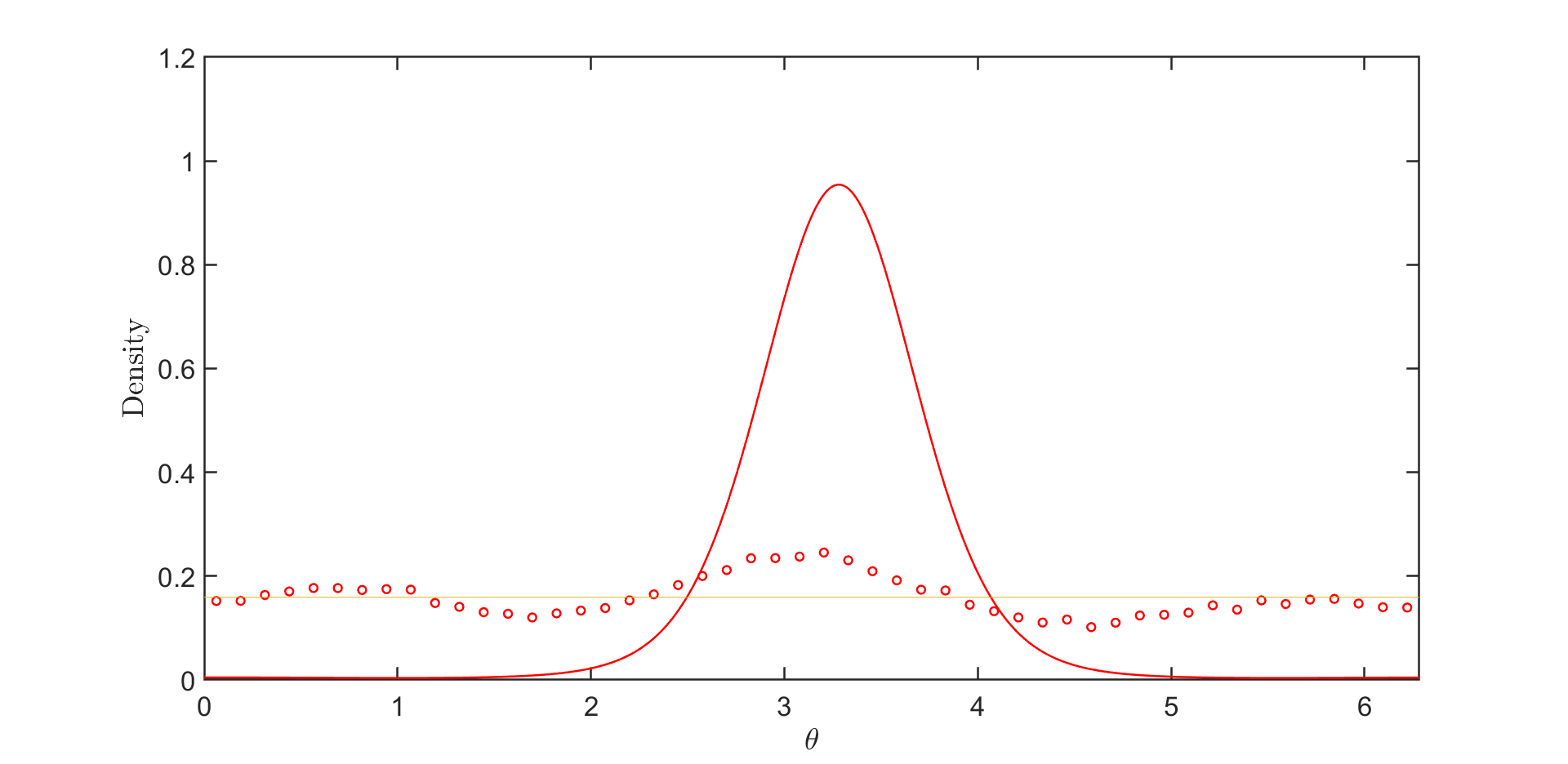
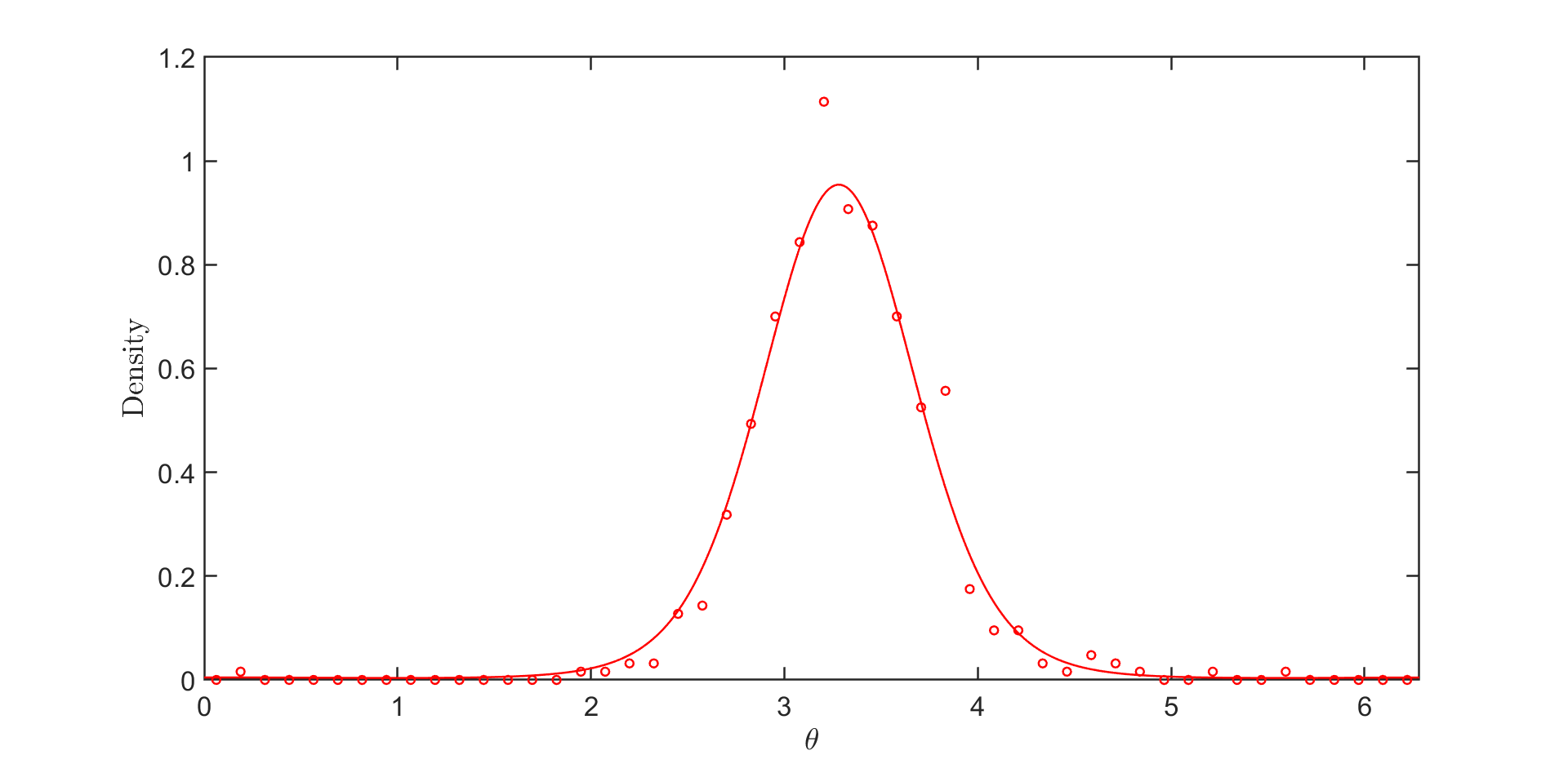
Figure 8: PDE and SDE dynamics for $W(x)=-\cos(x)-\frac{1}{2}\cos(2x)$ for 500 particles and 100 runs (left) and 1 run (right).

We now compare the PDE and SDE dynamics for a range of other interactions and no external potential. Our next example concerns the interaction potential $W(x)=-\frac{1}{4}\cos(4x)-\frac{1}{6}\cos(6x)$, and is chosen to demonstrate the agreement for multi-peaked solutions. We integrate up to $T=200$, with a timestep $\Delta t=0.01$. As can be seen in Figure 9, the agreement between the PDE and SDE is very good. Note that here we did not need to shift the PDE solution to align the peaks; this would not be true for a different realisation of the noise.

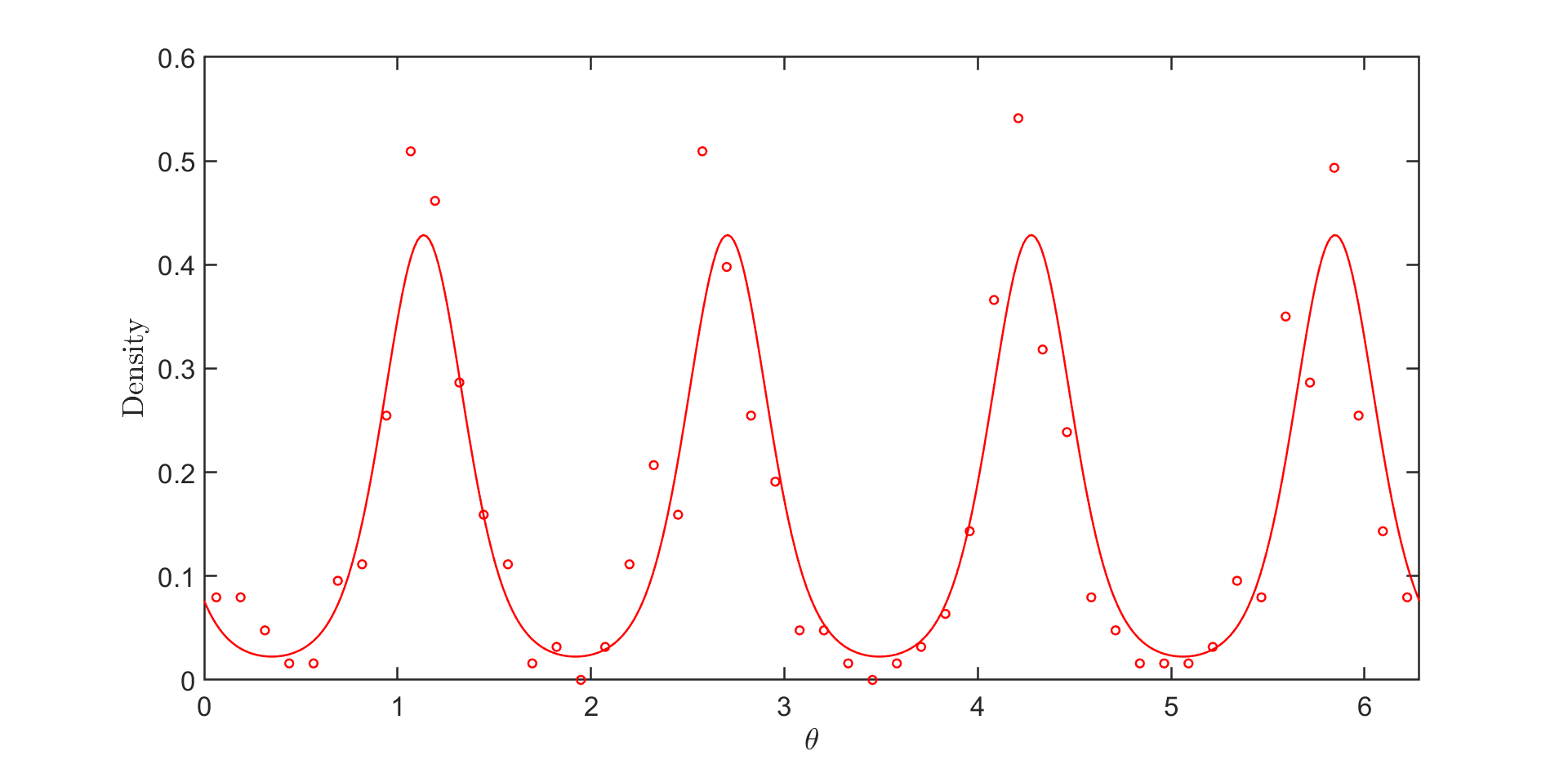
Figure 9: PDE and SDE dynamics with one run for $W(x)=-\frac{1}{4}\cos(4x)-\frac{1}{6}\cos(6x),V(x)=0,\beta=10$.

Our next example is chosen from [35] concerning Hodgkin-Huxley oscillators, where the second Fourier mode now has positive sign. We take $W(x)=-\cos(x)+\frac{1}{2}\cos(2x)$. Our numerical experiments (not shown) agree with the result of the paper that there is a phase transition at $\beta_{c}=2$. We plot here the density for $\beta=3$, with $100$, T = $200$, and $\Delta t=0.01$. The results are shown in Figure 10; again, the agreement between the SDE and PDE is very good.

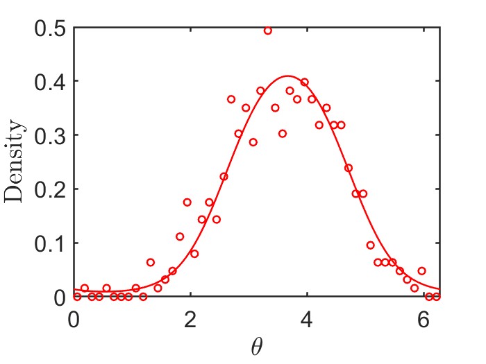
Figure 10: PDE and SDE dynamics for $W(x)=-\cos(x)+\frac{1}{2}\cos(2x),V(x)=0,\beta=3$.

In contrast to the examples presented so far, the presence of an external/confining potential breaks translation invariance. Consequently, averaging over many realization of the noise in the particle simulations leads to a non-uniform stationary state. We now consider two such examples, averaging solutions for 500 particles over 10 runs in each case.

For the first example we consider the Brownian mean field model in a magnetic field, (7), with $W(x)=-\cos(x)$ and $V(x)=0.2\cos(x+\pi)$. We integrate up to $T=1000$ with $\Delta t=0.01$. The results are shown in Figure 11, where we once again have excellent agreement between the PDE and SDE.

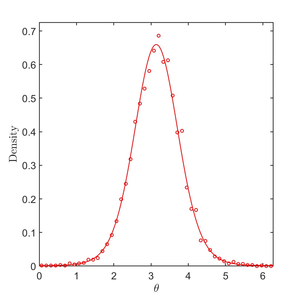
Figure 11: PDE and SDE dynamics for $W(x)=-\cos(x)$ with confining potential $V(x)=0.2\cos(x+\pi),\beta=3$, 500 particles, 10 runs.

Finally for long time solutions, we consider an example taken from [1]. Here $W(x)=-2\cos(2x)$ and $V(x)=\cos(x)$. In this case the dynamics converge more slowly and we take a final time of $T=7000$ and $\Delta t=0.01$. Figure 12 demonstrates the excellent agreement between the dynamics at long times.

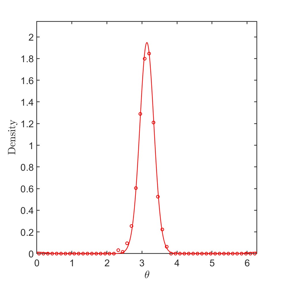
Figure 12: PDE and SDE dynamics for $W(x)=-2\cos(x)$ with confining potenital $V(x)=\cos(x+\pi),\beta=3,500$ particles.

Of course, one is often interested not only in long time dynamics, but also in the full evolution of the density. In Figure 13 we compare the PDE and SDE dynamics at a number of times for two different combinations of interaction and external potentials. As previously discussed, the agreement between the two dynamics is better in the second picture as we have a confining potential which breaks translation invariance, and a simpler interaction potential.

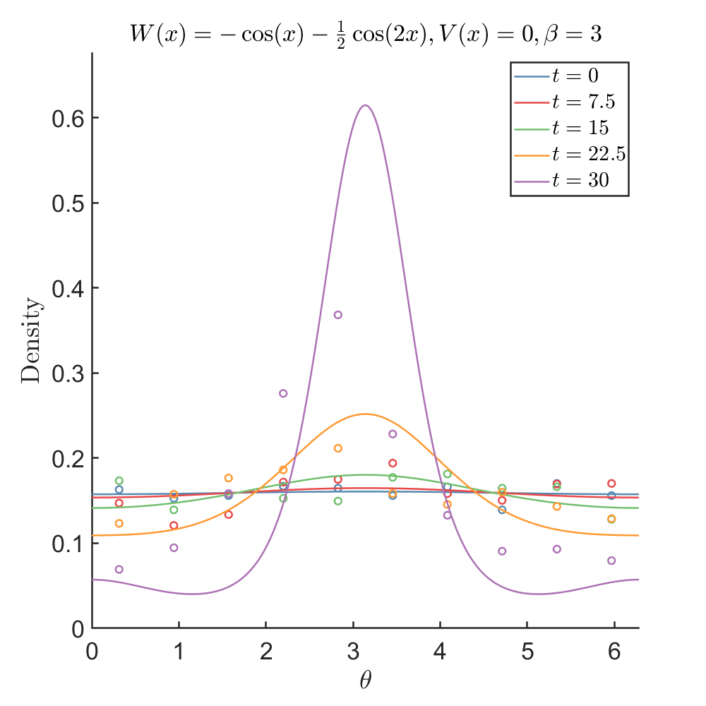
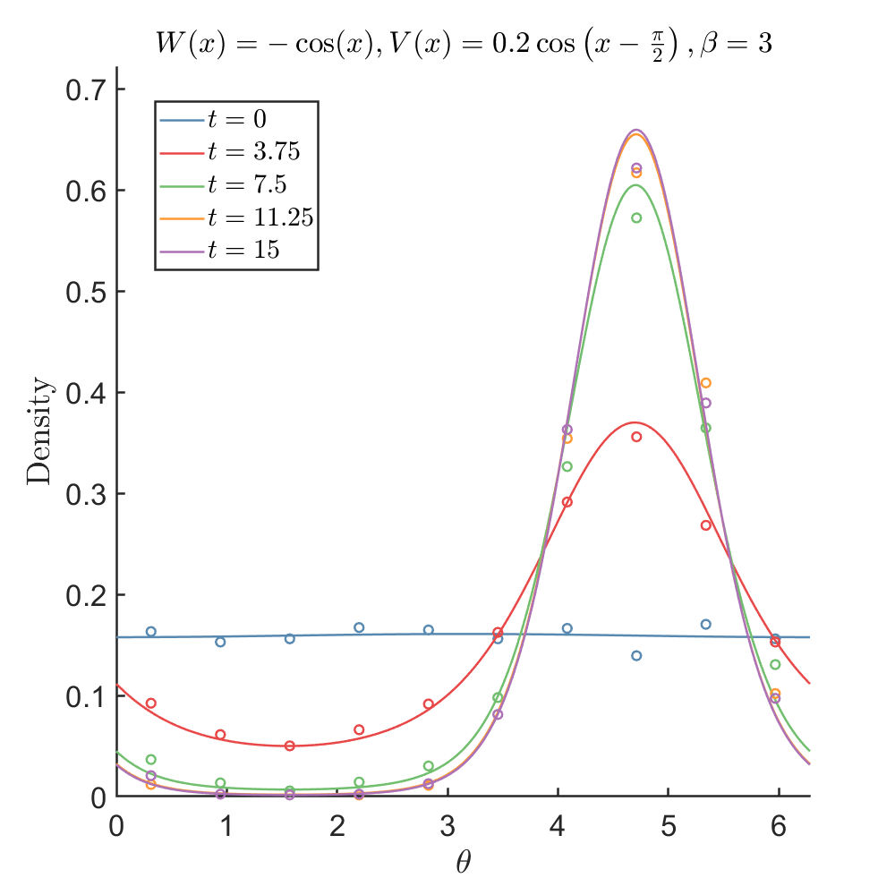
Figure 13: PDE and SDE dynamics for a different range of times, $\beta=3$, for $W(x)=-\cos(x)-\frac{1}{2}\cos(2x),V(x)=0$ (left) and for $W(x)=-\cos(x)$, $V(x)=0.2\cos\left(x-\frac{\pi}{2}\right)$ (right).

5.3 PDE simulations for the HKB model

Another model with confining potential is the Haken–Kelso–Bunz (HKB) (see Chapter 5, [18]). Here $W(x)=-\cos(x)$, $V(x)=-\alpha\cos(x+\pi)-\gamma\cos(2x)$. We plot the stationary states of the Fokker-Planck PDE for different values of $\alpha,\gamma$.

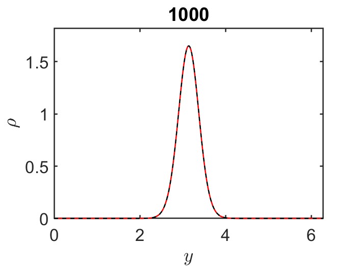
Figure 14: PDE dynamics for the HKB model with $\alpha,\gamma=1$, $\beta=3$.

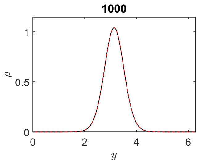
Figure 15: PDE dynamics for the HKB model with $\alpha=1,\gamma=\frac{1}{8}$, $\beta=3$.

6 Conclusions

In this paper, we studied the stability of steady states for McKean-Vlasov dynamics on the torus, for interaction potentials that contain multiple non-zero Fourier modes. It was shown, through the study of the self-consistency equations, of the free energy of the system and through a linear stability analysis, that there is a critical temperature value at which the constant stationary state of the system becomes unstable. Furthermore, the stability of non-constant stationary states was analysed by means of perturbation theory for higher harmonic and multichromatic interaction potentials. Finally, we verified these results with extensive numerical simulations of both the Fokker-Planck PDEs and the systems of SDEs involved.

The work presented in this paper can be extended in several interesting directions. First, we would like to study the effect of inertia on the formation and stability of multipeak solutions by considering the kinetic mean field PDE. Second, the impact of colored noise on the stability on the phase transitions and on the stability of non-uniform steady states is an important question, motivated by recent work on the modeling of collective organization in cyanobacteria [15]. More generally, we aim at applying our analytical and numerical methodologies to the study of active matter, e.g. [32]. All these topics are currently under investigation.

Acknowledgments

BB is funded by a studentship from the Imperial College London EPSRC DTP in Mathematical Sciences (Grant No. EP/W523872/1) and was supported by a Mary Lister McCammon summer research fellowship. GP is partially supported by an ERC-EPSRC Frontier Research Guarantee through Grant No. EP/X038645, ERC through Advanced Grant No. 247031.

References

- [1] L. Angeli, J. Barré, M. Kolodziejczyk and M. Ottobre “Well-posedness and stationary solutions of McKean-Vlasov (S) PDEs” In Journal of Mathematical Analysis and Applications 526.2 Elsevier, 2023, pp. 127301
- [2] R. Balescu “Statistical dynamics. Matter out of equilibrium” London: Imperial College Press, 1997
- [3] G. A. Battle “Phase transitions for a continuous system of classical particles in a box” In Comm. Math. Phys. 55.3, 1977, pp. 299–315 DOI: 10.1007/BF01614553
- [4] F. Bavaud “Equilibrium properties of the Vlasov functional: the generalized Poisson-Boltzmann-Emden equation” In Rev. Modern Phys. 63.1, 1991, pp. 129–148 DOI: 10.1103/RevModPhys.63.129
- [5] L. Bertini, G. Giacomin and K. Pakdaman “Dynamical aspects of mean field plane rotators and the Kuramoto model” In Journal of Statistical Physics 138 Springer, 2010, pp. 270–290
- [6] J. Binney and S. Tremaine “Galactic Dynamics” Princeton: Princeton University Press, 2008
- [7] J.P. Boyd “Chebyshev and Fourier spectral methods” Courier Corporation, 2001
- [8] J. A. Carrillo, M. G. Delgadino and G. A. Pavliotis “A -convexity based proof for the propagation of chaos for weakly interacting stochastic particles” In J. Funct. Anal. 279.10, 2020, pp. 108734 DOI: 10.1016/j.jfa.2020.108734
- [9] J. A. Carrillo, R. S. Gvalani, G. A. Pavliotis and A. Schlichting “Long-time behaviour and phase transitions for the Mckean-Vlasov equation on the torus” In Arch. Ration. Mech. Anal. 235.1, 2020, pp. 635–690 DOI: 10.1007/s00205-019-01430-4
- [10] P. Chavanis “The Brownian mean field model” In The European Physical Journal B 87 Springer, 2014, pp. 1–33
- [11] P. Constantin, I. G. Kevrekidis and E. S. Titi “Asymptotic states of a Smoluchowski equation” In Arch. Ration. Mech. Anal. 174.3, 2004, pp. 365–384 DOI: 10.1007/s00205-004-0331-8
- [12] F. A. Davidson and N. Dodds “Spectral properties of non-local differential operators” In Appl. Anal. 85.6-7, 2006, pp. 717–734 DOI: 10.1080/00036810600555171
- [13] F. A. Davidson and N. Dodds “Spectral properties of non-local uniformly-elliptic operators” In Electron. J. Differential Equations, 2006, pp. No. 126, 15
- [14] M. G. Delgadino, R. S. Gvalani and G. A. Pavliotis “On the Diffusive-Mean Field Limit for Weakly Interacting Diffusions Exhibiting Phase Transitions” In Arch. Ration. Mech. Anal. 241.1, 2021, pp. 91–148 DOI: 10.1007/s00205-021-01648-1
- [15] M. K. Faluweki, J. Cammann, M. G. Mazza and L. Goehring “Active Spaghetti: Collective Organization in Cyanobacteria” In Phys. Rev. Lett. 131 American Physical Society, 2023, pp. 158303 DOI: 10.1103/PhysRevLett.131.158303
- [16] I. Fatkullin and V. Slastikov “A note on the Onsager model of nematic phase transitions” In Commun. Math. Sci. 3.1, 2005, pp. 21–26 URL: http://projecteuclid.org/euclid.cms/1111095638
- [17] I. Fatkullin and V. Slastikov “Critical points of the Onsager functional on a sphere” In Nonlinearity 18.6, 2005, pp. 2565–2580 DOI: 10.1088/0951-7715/18/6/008
- [18] T.D. Frank “Nonlinear Fokker-Planck equations”, Springer Series in Synergetics Berlin: Springer-Verlag, 2005, pp. xii+404
- [19] J. Garnier, G. Papanicolaou and T. Yang “Consensus convergence with stochastic effects” In Vietnam Journal of Mathematics 45 Springer, 2017, pp. 51–75
- [20] E. Geigant and M. Stoll “Stability of peak solutions of a non-linear transport equation on the circle” In Electronic Journal of Differential Equations 2012.157 Citeseer, 2012, pp. 1–41
- [21] B. D. Goddard, A. Nold and S. Kalliadasis “2DChebClass [Software]” Edinburgh DataShare, 2017 URL: http://dx.doi.org/10.7488/ds/1991
- [22] B. D. Goddard, B. Gooding, H. Short and G. A. Pavliotis “Noisy bounded confidence models for opinion dynamics: the effect of boundary conditions on phase transitions” hxab044 In IMA Journal of Applied Mathematics, 2021 DOI: 10.1093/imamat/hxab044
- [23] P.E. Kloeden and E. Platen “Numerical Solution of Stochastic Differential Equations”, Stochastic Modelling and Applied Probability Springer Berlin Heidelberg, 2013 URL: https://books.google.co.uk/books?id=r9r6CAAAQBAJ
- [24] D. Lacker “Hierarchies, entropy, and quantitative propagation of chaos for mean field diffusions” In Probab. Math. Phys. 4.2, 2023, pp. 377–432 DOI: 10.2140/pmp.2023.4.377
- [25] M. Lucia and J. Vukadinovic “Exact multiplicity of nematic states for an Onsager model” In Nonlinearity 23.12, 2010, pp. 3157–3185 DOI: 10.1088/0951-7715/23/12/009
- [26] N. Martzel and C. Aslangul “Mean-field treatment of the many-body Fokker-Planck equation” In J. Phys. A 34.50, 2001, pp. 11225–11240 DOI: 10.1088/0305-4470/34/50/305
- [27] R. M. Neal “Slice sampling” In The annals of statistics 31.3 Institute of Mathematical Statistics, 2003, pp. 705–767
- [28] A. Nold et al. “Pseudospectral methods for density functional theory in bounded and unbounded domains” In J. Comput. Phys. 334 Elsevier, 2017, pp. 639–664
- [29] K. Oelschlager “A martingale approach to the law of large numbers for weakly interacting stochastic processes” In The Annals of Probability JSTOR, 1984, pp. 458–479
- [30] K. J. Painter, T. Hillen and J. R. Potts “Biological modeling with nonlocal advection-diffusion equations” In Math. Models Methods Appl. Sci. 34.1, 2024, pp. 57–107 DOI: 10.1142/S0218202524400025
- [31] G. A. Pavliotis “Stochastic processes and applications” Diffusion processes, the Fokker-Planck and Langevin equations 60, Texts in Applied Mathematics Springer, New York, 2014, pp. xiv+339 DOI: 10.1007/978-1-4939-1323-7
- [32] F. Peruani, A. Deutsch and M. Bär “A mean-field theory for self-propelled particles interacting by velocity alignment mechanisms” In The European Physical Journal Special Topics 157 Springer, 2008, pp. 111–122
- [33] I. Primi, A. Stevens and J.L. Velazquez “Mass-selection in alignment models with non-deterministic effects” In Communications in Partial Differential Equations 34.5 Taylor & Francis, 2009, pp. 419–456
- [34] J. Vukadinovic “Inertial manifolds for a Smoluchowski equation on the unit sphere” In Comm. Math. Phys. 285.3, 2009, pp. 975–990 DOI: 10.1007/s00220-008-0460-2
- [35] J. Vukadinovic “Phase transition for the McKean-Vlasov equation of weakly coupled Hodgkin-Huxley oscillators” In Discrete and Continuous Dynamical Systems DiscreteContinuous Dynamical Systems, 2023, pp. 0–0