Approximate Bayesian Computation with Deep Learning and Conformal prediction

Abstract

Approximate Bayesian Computation (ABC) methods are commonly used to approximate posterior distributions in models with unknown or computationally intractable likelihoods. Classical ABC methods are based on nearest neighbor type algorithms and rely on the choice of so-called summary statistics, distances between datasets and a tolerance threshold. Recently, methods combining ABC with more complex machine learning algorithms have been proposed to mitigate the impact of these "user-choices". In this paper, we propose the first, to our knowledge, ABC method completely free of summary statistics, distance and tolerance threshold. Moreover, in contrast with usual generalizations of the ABC method, it associates a confidence interval (having a proper frequentist marginal coverage) with the posterior mean estimation (or other moment-type estimates).

Our method, ABCD-Conformal, uses a neural network with Monte Carlo Dropout to provide an estimation of the posterior mean (or others moment type functional), and conformal theory to obtain associated confidence sets. Efficient for estimating multidimensional parameters, we test this new method on three different applications and compare it with other ABC methods in the literature.

Keywords: Likelihood-free inference · Approximate Bayesian computation · Convolutional neural networks · Dropout · Conformal prediction · probability matching criterion.

1 Introduction

In many situations, the likelihood function plays a key role in both frequentist or Bayesian inference. However, it is not unusual that such likelihood is difficult to work with either because no closed form expression exists, e.g., the corresponding statistical model is too complex, or because its computational cost is prohibitive. For example, the first situation occurs with max-stable processes [de Haan,, 1984] or Gibbs random fields [Besag,, 1974; Grelaud et al.,, 2009], while the second case frequently occurs with mixture models [Simola et al.,, 2021].

In this paper, we will restrict our attention to parameter inference in the Bayesian framework and in particular to Approximate Bayesian Computation (ABC), which is one of the most popular likelihood-free parameter inference method. Indeed, ABC can be an efficient alternative to overcome the situation of intractable likelihood functions [Marin et al.,, 2012]. Within the ABC framework, the need for computing the likelihood function is substituted by the need to be able to simulate from the statistical model under consideration. The first proposed ABC methods enabled to obtain an approximation of the posterior distribution of interest, from simulations [Pritchard et al.,, 1999]. For these early methods, the degree of approximation depends strongly on the choices of the tolerance threshold, the distance and of the so-called summary statistics used during the ABC estimation. Unfortunately, identifying the most relevant summary statistics is problem dependent and in many situations the statistics are chosen by the practitioner, even if several studies provide guidance in this choice, see for instance Joyce and Marjoram, [2008], McKinley et al., [2009], Blum et al., [2012], Fearnhead and Prangle, [2012] among others.

Recently, several approaches managed to mitigate the need of identifying relevant summary statistics. These approaches combine the ABC framework with machine learning methods, such as random forests or neural networks. For instance, Raynal et al., [2018] propose an automatic selection of relevant summary statistics. They propose to consider a large set of potentially relevant summary statistics and use the random forest framework as a black box to get some point estimates of the posterior distribution given these summary statistics. Another approach of interest is the one of Akesson et al., [2022], which uses the estimated posterior mean as a summary statistic, this posterior mean being estimated through a Convolutional Neural Network (CNN). Consequently, since the emergence of ABC methods, a wide variety of methods have been proposed, from the standard "basic" ABC to methods using random forests or neural networks, and including those using MCMC or filtering algorithms (see Marjoram et al., [2003], Sisson et al., [2007], Baragatti and Pudlo, [2014] and references therein).

To quantify the uncertainties, Bayesian methods provide posterior credible intervals from the posterior distribution, through posterior quantiles or highest posterior density regions. This can be justified because, in many simple parametric models, the Bernstein-von Mises theorem ensures that posterior credible intervals are asymptotically as well, reconciling the frequentist and Bayesian approaches. However, these credible intervals are not necessarily relevant in practice. Indeed, note for instance that in nonparametric and high-dimensional models, research is still ongoing to understand better the link between the coverage of credible intervals and the coverage of frequentist , see Rousseau and Szabo, [2016]; Datta et al., [2000]; Hoff, [2023] among others. Indeed, the posterior coverage probability of a Bayesian credible interval does not always match with the corresponding frequentist coverage probability. Quite often, they can even diverge in nontrivial ways, see for instance Wasserman, [2011]. In this case, we say that the probability matching criterion is not verified. This criterion can be hard to check when the exact posterior distribution is known, and even more so when the posterior is approximated [Frazier et al.,, 2018], which is the cases of most applications requiring an ABC method. Another drawback of using posterior credible intervals in ABC methods is that they only take into account the inherent randomness of the model when estimating the prediction uncertainty. Nevertheless, by definition of the method, the a posteriori distribution is approximated, so there is an error due to the method to take into account.

Our contribution.

In this paper, we propose a new ABC implementation that does not require summary statistics, tolerance threshold and distance. Our method produce point estimates of the posterior distribution e.g. mean, variance, quantiles, without aiming to approximate the whole posterior distribution. It also provide associated confidence sets of the estimates. The estimates are obtained using neural networks with Monte Carlo Dropout while the confidence sets are obtained through conformal prediction. Our ABC estimation method only requires a 1) sampling function, 2) a neural network (NN) whose architecture is tailored for the problem of interest e.g. CNN for images, GNN for data with a graph structure, RNN for sequential data, and 3) a confidence level. While 1) and 3) are common to all ABC methods, requirement 2) is more original, but still easy to implement because well known architectures can be used with minimal changes, i.e. the inclusion of Dropout (or concrete Dropout) layers. Another originality of this work is that it produces directly confidence sets with proper marginal coverage.

We test the proposed ABCD-conformal algorithm in three different problems. We compare the results against the standard ABC, the ABC Random Forest (ABC-RF) of Raynal et al., [2018] and the ABC-CNN of Akesson et al., [2022]. We measure both the accuracy of the estimation and the frequentist coverage of confidence sets.

The paper is organized as follows. In section 2 we briefly present some existing ABC methods: standard ABC, ABC-CNN and ABC-RF. In section 3, we propose the ABCD-conformal methodology, combining neural networks and conformal prediction in a likelihood-free framework. Then, we illustrate and compare all these methods on three examples in section 4, before a discussion in section 5.

2 A few approaches of Approximate Bayesian Computation

2.1 Standard ABC: assets and drawbacks

Consider a parametric statistical model $\{f(x\mid\theta)\colon x\in\mathbb{R}^{d},\theta\in\Theta\}$ on which we assume a prior distribution $\pi$ on the parameter $\theta$ leading to the Bayesian parametric model $\{f(\cdot\mid\theta),\pi\}$. Based on the sample $\mathbf{x}=(x_{1},\ldots,x_{n})$, the cornerstone of any Bayesian inference is the posterior distribution

$$\pi(\theta\mid\mathbf{x})=\frac{f(\mathbf{x}\mid\theta)\pi(\theta)}{\int_{\Theta}f(\mathbf{x}\mid\theta)\pi(\theta)\mbox{d$\theta$}}\propto f(\mathbf{x}\mid\pi)\pi(\theta),$$ (1)

where $f(\mathbf{x}\mid\theta)$ denotes the likelihood function for the sample $\mathbf{x}$ and parameter $\theta$. In a setting where we assume that the likelihood is not tractable, the simple, standard ABC methodology was the first powerful algorithm to bypass this hurdle (see Pritchard et al., [1999] or Marin et al., [2012]) and, in one of its simplest form, is described in Algorithm 1.

1

Input : A Bayesian parametric model $\{f(\cdot\mid\theta),\pi\}$, a data sample $\mathbf{x}$, the size of the training set $N_{\text{train}}$, summary statistics $\eta:\mathbb{R}^{d}\to\mathbb{R}^{l}$, a (pseudo)-distance $d$ on $\mathbb{R}^{l}$, and a tolerance threshold $\alpha\in(0,1]$.

2

Output : A set $\theta_{1},\ldots,\theta_{[N_{\text{train}}\alpha]}$ whose distribution is approximately $\pi(\theta\mid\mathbf{x})$

3

4Generation of a reference table :

5 for $j\leftarrow 1$ to $N_{\text{train}}$ do

6       Draw $\theta_{j}\sim\pi$;

7      

8      Draw synthetic sample $\mathbf{x}_{j}=(x_{1,j},\ldots,x_{d,j})^{\top}$ from the model $f(\cdot\mid\theta_{j})$ 

9 end for

10Summary statistics and distances :

11 for $j\leftarrow 1$ to $N_{\text{train}}$ do

12       Compute the vector of summary statistics $\eta(\mathbf{x}_{j})$;

13      

14      Compute the (pseudo)-distance $d_{j}=d(\eta(\mathbf{x}),\eta(\mathbf{x}_{j}))$ 

15 end for

16

17Order these distances, i.e., $d_{(1)}<d_{(2)}<\cdots<d_{(N_{\text{train}})}$;

18

Keep the $\theta_{j}$ corresponding to the $\lfloor N_{\text{train}}\alpha\rfloor$ smallest distances.

Algorithm 1 Pseudo code for the standard ABC sampler

In Algorithm 1, $d$ is typically a pseudo distance of the form

$$d\colon\mathbb{R}^{l}\times\mathbb{R}^{l} \longrightarrow\mathbb{R}_{+}$$

$$(\eta(\mathbf{x}),\eta(\mathbf{x})) \longmapsto\|\eta(\mathbf{x})-\eta(\mathbf{x})\|,$$

where $\eta$ summarizes the data and is called the vector of summary statistics. $\|\cdot\|$ is typically the usual Euclidean norm.

This algorithm samples $\theta$ and $\mathbf{x}$ from the joint posterior density

$$\pi_{\alpha,d}(\theta,\mathbf{x}\mid\eta(\mathbf{x}))=\frac{\pi(\theta)f(\mathbf{x}\mid\theta)\mathbf{1}_{\alpha,d}(\mathbf{x})}{\int\pi(\theta)f(\mathbf{x}\mid\theta)\mathbf{1}_{\alpha,d}(\mathbf{x})d\mathbf{x}d\theta},$$

where $\mathbf{1}_{\alpha,d}(\mathbf{x})=\mathbf{1}\big{[}d\big{(}\eta(\mathbf{x}),\eta(\mathbf{x})\big{)}<d_{([\alpha N]+1)}\big{]}$. The approximate Bayesian computation posterior density is defined as:

$$\pi_{\alpha,d}(\theta\mid\eta(\mathbf{x}))=\int\pi_{\alpha,d}(\theta,\mathbf{x}\mid\eta(\mathbf{x}))d\mathbf{x}$$

The basic idea behind ABC is that using a representative (enough) summary statistic $\eta$ coupled with a small (enough) tolerance $\alpha$ should produce a good (enough) approximation to the posterior distribution; that is $\pi_{\alpha,d}(\theta\mid\eta(\mathbf{x}))\approx\pi(\theta\mid\mathbf{x})$. This approximation has been validated by different theoretical results. Let us cite the work of Frazier et al., [2018] which prove that the posterior distribution concentrates on sets containing the true parameter under general assumptions and with some rates of convergence. Cite also Fearnhead and Prangle, [2012] which describe the best summary statistics to perform this approximation.

Nevertheless, for the algorithm to give a valid approximation of the true posterior distribution, not only $\pi_{\alpha,d}$ has to be close to $\pi$, but also the Monte Carlo approximation error :

$$\frac{1}{\lfloor N\alpha\rfloor}\sum_{j,d_{j}\leq d_{(\lfloor N\alpha\rfloor)}}\delta_{\widetilde{\theta_{j}}}\approx\pi_{\alpha,d}$$ (2)

needs to be considered. In Eq. (2), $d_{j}$ and $d_{(.)}$ are defined in Algorithm 1. Here it only corresponds to the rate of convergence of the empirical measure in the classical law of large number. This question has recently attracted a great deal of attention Fournier and Guillin, [2015]; Dereich et al., [2013]; Weed and Bach, [2019]. There is a unavoidable curse of dimensionality : the empirical measure over a $n$-sample (here $n=\lfloor N\alpha\rfloor$) is at distance $n^{-1/d}$ to the target measure. This explain why the standard ABC lacks efficiency when the dimension of $\mathbf{x}$ is large or when the dimension of the summaries is large. This also induces high computation times. Using a small number of relevant summaries is then crucial, but, when the size of the data tends to infinity, these summaries should converge toward an injective mapping from parameters to summaries. This injectivity depends on both the true structural model and the particular choice of $\eta(\cdot)$, hence there is no general method for finding such statistics $\eta(\cdot)$. This can restrict the (computational) use or the validity of the standard ABC algorithm, because without this condition posterior concentration is not guaranteed.

2.2 Towards a preprocessing summary statistics free ABC

In this section, we briefly review two attempts in the ABC literature to obtain methods depending less on the summary statistics choice (and distance) than the original ABC method.

2.2.1 ABC-Convolutional Neural Network (Akesson et al., [2022])

The earliest work to bypass the choice of summary statistics in the ABC method is maybe the one of Fearnhead and Prangle, [2012]. Indeed, they showed that the optimal summary statistic is the true posterior mean of the parameter of interest. Although it cannot be calculated analytically, they proposed an extra stage of simulation to estimate it. This estimates is then used as a summary statistic within a standard ABC algorithm. In practice, they used linear regression to estimate the posterior mean, with appropriate functions of the data as predictors. This approach has inspired Jiang et al., [2017] who proposed to estimate the posterior means using deep Neural Networks (NN) instead of linear regression. Akesson et al., [2022] goes a bit further by proposing to estimate them using Convolutional Neural Networks (CNN). Indeed, CNNs are often more effective than classical dense NNs for tasks involving structured grid data, such as images, audio, video and time-series data (see for example LeCun et al., [1999] or Boston et al., [2022]). The approach of Akesson et al., [2022] is then a slight modification of the standard ABC: CNN are used to estimate the posterior mean of a parameter, which is then used as a summary statistic. Hence to have asymptotic consistency and valid frequentist coverages, the same kind of conditions are needed than for Algorithm 1. For sake of completeness, this algorithm is briefly described and commented in appendix, see Algorithm 3.

2.2.2 ABC-Random Forest [Raynal et al.,, 2018]

Another interesting approach is the one of Raynal et al., [2018]. Their goal is slightly different from the goal of standard ABC, as they do not seek to approximate the full posterior distribution. Instead, they focused on functional of the posterior distribution, like posterior mean, posterior variance or posterior quantiles. Indeed, they are easier to interpret and report than the whole posterior distribution, and are the main interest of practitioners. Formally, they predict a scalar transform $T(\theta)$ of a multidimensional parameter $\theta$. Without loss of generality, their interest is in

$$\psi(\mathbf{x})=\mathbb{E}_{\pi}[T(\theta)\mid\mathbf{x}]=\int_{\Theta}T(\theta)\pi(\theta\mid\mathbf{x})\mbox{d$\theta$}=c(\mathbf{x})\int_{\Theta}T(\theta)f(\mathbf{x}\mid\theta)\pi(\theta)\mbox{d$\theta$},$$ (3)

where $c(\mathbf{x})$ is a normalizing constant. From this functional, we easily recover posterior mean, posterior variance or posterior quantiles using respectively $T(\theta)=\theta$, $T(\theta)=\theta^{2}$ and $T(\theta)=\theta$, and $T(\theta)=\mathbf{1}_{\theta\leq q}$.

To mitigate the curse of dimensionality, the dimension of (3) can be reduced by using summary statistics, i.e., the focus is now on

$$\psi_{\eta}(\mathbf{x})=\mathbb{E}_{\pi}[T(\theta)\mid\eta(\mathbf{x})]=\int_{\Theta}T(\theta)\pi\{\theta\mid\eta(\mathbf{x})\}\mbox{d$\theta$}=c_{\eta}(\mathbf{x})\int_{\Theta}T(\theta)f\{\eta(\mathbf{x})\mid\theta\}\pi(\theta)\mbox{d$\theta$},$$ (4)

which is hoped to be a good approximation of $\psi(\mathbf{x})$ but much simpler to estimate. Although many studies focus on how to calculate efficiently an average from a sample see for example Gobet et al., [2022] and references therein, the idea of directly approximating the functional of interest in Eq. (3) (or similarly in Eq. (4)) bypasses the costly step of approximating the empirical measure Eq. (2), especially when the dimension is large.

Raynal et al., [2018] then proposed approximations of $\psi_{\boldsymbol{\eta}}(\mathbf{x})$, of the posterior variance $\mathbb{V}_{\pi}[T(\theta)\mid\eta(\mathbf{x})]$ and of posterior quantiles, using (regression) random forests [Breiman,, 2001]. Their algorithm is briefly described and commented in Algorithm 4. A drawback of this method (as presented in Raynal et al., [2018] ) is that it only works on unidimensional parameter inference. When the parameter $\theta$ of interest is multidimensional, Raynal et al., [2018] recommend to construct one random forest (RF) for each unidimensional component of $\theta$, and covariance between components is not taken into account. Additional RFs might be constructed if one is interested by estimating posterior covariance between pairs of components. Piccioni et al., [2022] used for instance this approach with an additional sensitivity analysis. To quantify the uncertainty of their estimation, Raynal et al., [2018] proposes, as usual, to use their approximated estimation of quantiles and variances (in Raynal et al., [2018, Section 2.3.3]) but also to use the so-called out-of-bag simulations inherent from RF algorithms (in Raynal et al., [2018, Section 2.3.4]). This latter gives a first hint to quantify uncertainty without giving nevertheless precise confidance intervals.

3 The ABCD-conformal algorithm

In this section we propose a new ABC method based on Deep learning with Dropout and conformal prediction, entitled ABCD-conformal.

3.1 Motivation and principle

Like Raynal et al., [2018], instead of approximating the whole posterior $\pi(\theta\mid\mathbf{x})$, we are interested in estimating functional of the form $\psi(\mathbf{x})=\mathbb{E}_{\pi}[T(\theta)\mid\mathbf{x}]$ (see equation Eq. (3)). The ABCD-conformal method will both output a prediction and an associated exact confidence interval.

Our method uses Neural Networks (NN), similarly to Akesson et al., [2022]. However, in contrast to their approach, the NN directly outputs the functional of interest and an associated uncertainty, enabling us to bypass the nearest neighbors step detailed in Section 2.1 to overcome the shortcomings of standard ABC.

To use conformal prediction, we need both a prediction and an associated measure of uncertainty that we will name heuristic uncertainty and denote $\widehat{\mathbb{V}}(\mathbf{x})$. To this end, we will use neural networks with Dropout layers. Dropout layers are classically used to prevent overfitting for neural networks, see Hinton et al., [2012] and Srivastava et al., 2014a . However, they can also be used to associate uncertainties e.g. variance with predictions from neural networks, see the Bayesian Neural Network literature [Gal,, 2016]. We can then obtain valid confidence sets using these uncertainties through conformal prediction [Angelopoulos and Bates,, 2023]. These two steps are described in Sections 3.2 and 3.3.

3.2 Prediction and heuristic uncertainty using Monte Carlo Dropout

For an introduction to Deep Learning, we refer the reader to Courville et al., [2016]; Guéron, [2019] and references therein. Neural networks have a strong predictive power however they are often regarded as black boxes making their predictions not explainable and without uncertainty. This is an issue in many areas like medicine or autonomous vehicles where false predictions can have big consequences Filos et al., [2020].

A lot of efforts have been made recently either to explain predictions, see the Explainable AI [Xu et al.,, 2019; Dantas et al.,, 2023] literature or to associate an uncertainty with the prediction, see Izmailov et al., [2021] or Kompa et al., [2021] among many others approaches.

In this paper we focus on the Dropout method proposed in Gal, [2016] and Gal and Ghahramani, [2016] even if more recent uncertainty methods might be more powerful as for example Variational BNN methods Folgoc et al., [2021]; Jospin et al., [2022]. We choose the classical Dropout method as it is generic, simple to implement and to integrate into an already existing NN architecture. As explained in Section 3.3, using conformal prediction will enable us to compensate the shortcomings of Dropout.

At every training step, Dropout layers randomly drop (set to zero) some neurons (elements of the weights matrices) [Hinton et al.,, 2012; Srivastava et al., 2014b, ] according to some user-choice parameters (such as the Dropout probability). This mechanism prevents complex co-adaptations on the training data: an input or hidden unit cannot rely on other hidden units being present, this can also be seen as a regularization method during the training, to prevent overfitting. Standard Dropout layers are deactivated during test/prediction phase. In their seminal paper Gal and Ghahramani, [2016] proposed to activate Dropout during test, introducing randomness in the NN, hence in the ouput. Repeating the same prediction task several times produces a distribution and is sometimes called Monte Carlo Dropout (MC Dropout).

We briefly describe the MC Dropout procedure. Let $D=\{(\mathbf{x}_{j},\theta_{j}),j=1,\ldots,N\}$ be the training set, containing inputs $x$ and outputs $\theta$, where $x$ corresponds in the ABC framework to the sampled data and $\theta$ (or a transformation $T(\theta)$) to the unknown parameter of interest. The vector of parameters of the network (weights and bias) is denoted $\mathbf{\omega}$. During training, the goal is to find parameters of the network $\mathbf{\omega}$ that are likely to have generated the outputs $(\tilde{\theta}_{j},j=1,\ldots,N)$, given the inputs $(\mathbf{x}_{j},j=1,\ldots,N)$. For this goal, we use another Bayesian inference model to infer such $\omega$ and we then aim to estimate the distribution $\pi(\mathbf{\omega}\mid D)$. After training, the goal is then to predict the parameter of interest $\theta$ associated to a new $\mathbf{x}$.
The posterior distribution of interest is then:

$$\pi(\theta\mid\mathbf{x},D)=\int\pi(\theta\mid\mathbf{x},\mathbf{\omega})\pi(\mathbf{\omega}\mid D)d\mathbf{\omega}.$$ (5)

The density $\pi(\mathbf{\omega}\mid D)$ is quite complex and cannot be evaluated analytically. It is approximated using a variational approach by $q(\mathbf{\omega})$. The approximate posterior distribution of interest is then given by

$$q(\theta\mid\mathbf{x})=\int\pi(\theta\mid\mathbf{x},\mathbf{\omega})q(\mathbf{\omega})d\mathbf{\omega}.$$ (6)

The first two moments of this distribution can be estimated empirically following Monte Carlo integration with $K$ samples. For each Monte Carlo sample, different units of the network are randomly dropped out Hinton et al., [2012], we note $\widehat{\mathbf{\omega}_{k}}$ the estimated weights of the associated network with dropped units.

Hence, these weights $\widehat{\mathbf{\omega}_{k}}$ are different for each Monte Carlo iteration. Denote by $\mathbf{f}^{\mathbf{\omega}}(\mathbf{x})$ the model’s stochastic output for input $\mathbf{x}$ and parameters $\mathbf{\omega}$. Assuming that $\theta\mid\mathbf{x},\mathbf{\omega}\sim\mathcal{N}(\mathbf{f}^{\mathbf{\omega}}(\mathbf{x}),\tau^{-1}\mathbf{I})$ and $\widehat{\mathbf{\omega}_{k}}\sim q(\mathbf{\omega})$, $t=1,\ldots,K$; an unbiased (consistent) estimator for $\mathbb{E}_{q(\theta\mid\mathbf{x})}[\theta\mid\mathbf{x}]$ is given by:

$$\widehat{\theta}(\mathbf{x})=\frac{1}{K}\sum_{k=1}^{K}\mathbf{f}^{\widehat{\mathbf{\omega}_{k}}}(\mathbf{x}),$$ (7)

which corresponds to the average of $K$ stochastic forward passes through the network with Dropout. An unbiased (consistent) estimator for the second moment $\mathbb{E}_{q(\theta\mid\mathbf{x})}[\theta^{T}\theta]$ is given by:

$$\widehat{\mathbb{E}}[\theta^{T}\theta\mid\mathbf{x}]=\tau^{-1}\mathbf{I}+\frac{1}{K}\sum_{k=1}^{K}\mathbf{f}^{\widehat{\mathbf{\omega}_{k}}}(\mathbf{x})^{T}\mathbf{f}^{\widehat{\mathbf{\omega}_{k}}}(\mathbf{x})$$

Then to obtain a variance associated with the prediction of $\theta$ we can use the following unbiased (consistent) estimator:

$$\widehat{\mathbb{V}}[\theta\mid\mathbf{x}]=\underbrace{\tau^{-1}\mathbf{I}}_{\widehat{\mathbb{V}}_{a}[\theta\mid\mathbf{x}]}+\underbrace{\frac{1}{K}\sum_{k=1}^{K}\mathbf{f}^{\widehat{\mathbf{\omega}_{k}}}(\mathbf{x})^{T}\mathbf{f}^{\widehat{\mathbf{\omega}_{k}}}(\mathbf{x})-\widehat{\theta}(\mathbf{x})^{T}\widehat{\theta}(\mathbf{x})}_{\widehat{\mathbb{V}}_{e}[\theta\mid\mathbf{x}]},$$ (8)

which corresponds to the inverse model precision plus the sample variance of $K$ stochastic forward passes through the network with Dropout. Hence, using Dropout and its associated randomness, we can obtain an estimate of $\mathbb{E}_{q(\theta\mid\mathbf{x})}[\theta]$, as well as associated uncertainty. This estimate can be considered as an approximation of $\mathbb{E}_{\pi}[\theta]$ because $q(\theta\mid\mathbf{x})$ is an approximation of the posterior of interest $\pi(\theta\mid\mathbf{x},D)$. Moreover, Gal, [2016] interprets the uncertainty Eq. (8) as the sum of an aleatoric uncertainty $\widehat{\mathbb{V}}_{a}[\theta\mid\mathbf{x}]$ and an epistemic uncertainty $\widehat{\mathbb{V}}_{e}[\theta\mid\mathbf{x}]$. The aleatoric uncertainty $\widehat{\mathbb{V}}_{a}[\theta\mid\mathbf{x}]$ is interpreted as the noise in the data, it is the result of measurement imprecision (it is often modelled as part of the likelihood, and this is often a Gaussian corrupting noise). The epistemic uncertainty $\widehat{\mathbb{V}}_{e}[\theta\mid\mathbf{x}]$ is interpreted as the model uncertainty: uncertainty in the model parameters or in the structure of the model. The total predictive uncertainty $\widehat{\mathbb{V}}[\theta\mid\mathbf{x}]$ combines these both types of uncertainties and will be used as our heuristic uncertainty $\widehat{\mathbb{V}}(\mathbf{x})$.

In practice, for each of the $K$ Monte Carlo iterations, the weigths $\widehat{\mathbf{\omega}_{k}}$ are different, and the NN with input $\mathbf{x}$ gives as outputs $\mathbf{f}^{\widehat{\mathbf{\omega}_{k}}}(\mathbf{x})$ and $\tau_{\widehat{\mathbf{\omega}_{k}}}^{-1}$. The aleatoric uncertainty $\tau^{-1}$ is estimated by the mean of the $\tau_{\widehat{\mathbf{\omega}_{k}}}^{-1}$, and the epistemic uncertainty by the sample variance of the $\mathbf{f}^{\widehat{\mathbf{\omega}_{k}}}(\mathbf{x})$.

The main drawback of Dropout layers is that the Dropout probability is a new model hyperparameter. To circumvent this issue, Gal et al., [2017] propose a Dropout variant, called Concrete Dropout, that allows for automatic tuning of this probability in large models, using gradient methods. It improves performance and tunes automatically the Dropout rate, producing better uncertainties compared to classical Dropout. This is the Dropout version we will be using in the following.

Remark 1.

Gal, [2016] and Gal and Ghahramani, [2016] showed that optimising any neural network with Dropout is equivalent to a form of approximate inference in a probabilistic interpretation of the model. In other words, the optimal parameters found through the optimisation of a Dropout neural network are the same as the optimal variational parameters in a probabilistic Bayesian neural network with the same structure (the parameters are found through a variational inference approach). It means that a network trained with Dropout is equivalent to a Bayesian Neural Network and possesses all the properties of such a network (see MacKay, [1992] or Neal, [2012] concerning Bayesian Neural Networks). For this equivalence to be true, only one condition should be verified in the variational inference approach, which is about the Kullback-Leibler divergence between the prior distribution of the parameters $\mathbf{\omega}$ and an approximating distribution for $\mathbf{\omega}$. We will not need to verify such assumption because the theoretical guaranty of our confidence sets will be assured through the conformal prediction.

3.3 Conformal prediction

For a test input $\mathbf{x}$, the NN with concrete Dropout method enables us to obtain an approximation $\widehat{\theta}(\mathbf{x})$ of $\mathbb{E}_{\pi}[\theta\mid\mathbf{x}]$, as well as associated heuristic uncertainties $\widehat{\mathbb{V}}(\mathbf{x})$. However, it does not give valid confidence sets. In order to obtain such confidence sets, we propose to apply a conformal procedure, as explained in Angelopoulos and Bates, [2023]. Conformal prediction is indeed a straightforward way to generate valid confidence sets for wide variety of models from a proxy of the uncertainty. The better this proxy will be, the smaller confidence interval will be.

It requires a small amount of additional calibration data $\big{(}(\theta_{j},\mathbf{x}_{j}),j=1,\ldots,N_{\text{{cal}}}\big{)}$, hundreds of calibration data are theoretically enough (see Eq. (12) below). We propose to use as heuristic uncertainties $\widehat{\mathbb{V}}(\mathbf{x})$ one of the variances obtained from the NN with Dropout in Section 3.2, see Eq. (8).

This heuristic uncertainty can be transformed into a rigorous confidence interval $\mathcal{C}(\mathbf{x})$ through the following conformal procedure.

Using the heuristic uncertainty $\widehat{\mathbb{V}}(\mathbf{x})$, we compute a score $s(\theta,\mathbf{x})$ for each data sample in the calibration set, from these scores we can define $\widehat{q}$ the conformal quantile and then a confidence set. More precisely, as in Messoudi et al., [2022], the score function will be

$$s(\theta,\mathbf{x})=\sqrt{(\theta-\widehat{\theta}(\mathbf{x}))^{t}\widehat{\mathbb{V}}(\mathbf{x})^{-1}(\theta-\widehat{\theta}(\mathbf{x}))}.$$ (9)

We can then define $\widehat{q}$ as the $\frac{\lceil(N_{\text{cal}}+1)(1-\alpha)\rceil}{N_{\text{cal}}}$ quantile of $\big{\{}s(\theta_{j},\mathbf{x}_{j}),j=1,\ldots,N_{\text{{cal}}}\big{\}}$ to have as the confidence set :

$$\mathcal{C}(\mathbf{x})=\{\theta\ |\ s(\theta,\mathbf{x})\leq\widehat{q}\}.$$ (10)

This corresponds to an ellipsoid which center is $\widehat{\theta}(\mathbf{x})$ and covariance matrix is $\widehat{\mathbb{V}}(\mathbf{x})^{-1}/\widehat{q}^{2}$. In one dimension, we have $s(\theta,\mathbf{x})=|\theta-\widehat{\theta}(\mathbf{x})|/\sqrt{\widehat{\mathbb{V}}(\mathbf{x})}$, and

$$\mathcal{C}(\mathbf{x})=\Big{[}\widehat{\theta}(\mathbf{x})-\widehat{q}\sqrt{\widehat{\mathbb{V}}(\mathbf{x})};\widehat{\theta}(\mathbf{x})+\widehat{q}\sqrt{\widehat{\mathbb{V}}(\mathbf{x})}\Big{]}.$$ (11)

This confidence set satisfies the marginal coverage property, i.e. for a chosen $\delta\in[0,1]$ :

$$1-\delta\leq\mathbb{P}[\theta\in\mathcal{C}(\mathbf{x})]\leq 1-\delta+\frac{1}{N_{\text{{cal}}}+1}.$$ (12)

Indeed, see [Angelopoulos and Bates,, 2023, Appendix D] (in particular the right hand side inequality needs that random variables $s(\theta_{j},\mathbf{x}_{j})$ to be continuous). This probability is marginal over the randomness in the calibration and test points [Angelopoulos and Bates,, 2023], see Algorithm 2. One great advantage of this procedure is that it is easy to implement, fast and generic. Moreover, the obtained prediction intervals are non-asymptotic, with no distributional or model assumptions. The only assumption needed is that the calibration data and the test data are i.i.d [Vovk et al.,, 1999] which is naturally the case in our setting. Finally, this procedure provides a frequentist perspective on a Bayesian approach, reconciling the two points of view.
The performance of this approach in terms of intervals length depends only on the quality of the uncertainty measure used. A "good" uncertainty measure should reflect the magnitude of model error: it should be smaller for easy input, and larger for hard ones. If the uncertainty measure is "bad", then the intervals obtained by the conformal procedure will be quite large and their lengths will not differ a lot between easy and hard inputs. From the previous MC Dropout method, three types of uncertainties were obtained: epistemic, aleatoric and overall (sum of aleatoric and epistemic). In section 4, we show that depending on the examples, one or the other of these uncertainties will produce the best results.

Remark 2.

Note that a conditional coverage would be preferable, that is:

$$\mathbb{P}[\theta\in\mathcal{C}(\mathbf{x})\mid\mathbf{x}]\geq 1-\delta.$$ (13)

Indeed, marginal coverage does not guarantee the coverage of $\mathcal{C}(\mathbf{x})$ for any specific $\mathbf{x}$, only the average coverage over the whole domain. However, this conditional property is not guaranteed by the conformal procedure in general, but some metrics can be used to check how close we are to this stronger property, see Angelopoulos and Bates, [2023].

3.4 Implementation of ABCD-conformal

The training step of the proposed method is as follows. a) Generate the training dataset i.e. reference table in ABC vocabulary and the calibration dataset, of sizes $N_{\text{{train}}}$ and $N_{\text{{cal}}}$ respectively. b) The NN with Dropout is trained using the reference table. In principle, one could select the network architecture using an extra validation dataset. c) Monte Carlo Dropout prediction is performed, that is each sample of the calibration dataset is passed through the trained network with Dropout, $K$ times. For each of these samples, an approximation of $\mathbb{E}_{\pi}[\theta\mid\mathbf{x}]$ is obtained as the average of the $K$ predictions (see Eq. (7)), associated with an heuristic uncertainty which is here the variance, see Eq. (8). d) Using this approximation and associated uncertainty, the score of each sample of the calibration dataset is calculated. The conformal quantile is then the $\frac{\lceil(N_{\text{{cal}}}+1)(1-\delta)\rceil}{N_{\text{{cal}}}}$ quantile of the calibration scores.

Then, for a new data sample $\mathbf{x}$, to approximate $\mathbb{E}_{\pi}[\theta\mid\mathbf{x}]$ and obtain an associated confidence interval: e) Monte Carlo Dropout prediction is performed to obtain an approximation of $\mathbb{E}_{\pi}[\theta\mid\mathbf{x}]$ (average of the predictions) and the associated heuristic uncertainty (variance of the predictions). A confidence interval is then calculated using the conformal quantile calculated in d) Eq. (11).

The pseudo-code of the algorithm proposed is detailed in Algorithm 2.

1

Input : A Bayesian parametric model $\{f(\cdot\mid\theta),\pi\}$, a data sample $\mathbf{x}$, integers $N_{\text{{train}}}$, $N_{\text{{cal}}}$ and $K$ representing sizes of training and calibration sets, and the number of stochastic passes for the Dropout. $\delta$ between 0 and 1 to obtain $(1-\delta)$% confidence sets.

2

Output : An approximation of the posterior expected value $\mathbb{E}_{\pi}[\theta\mid\mathbf{x}]$ and a confidence interval for $\theta$.

3

4a) Generation of a reference table (training dataset) and a calibration dataset :

5 These datasets are of sizes $N_{\text{{train}}}$, $N_{val}$ and $N_{\text{{cal}}}$ respectively. For the reference table for instance:

6 for $j\leftarrow 1$ to $N_{\text{{train}}}$ do

7       Draw $\theta_{j}\sim\pi$;

8      

9      Draw synthetic sample $\mathbf{x}_{j}=(x_{1,j},\ldots,x_{d,j})^{\top}$ from the model $f(\cdot\mid\theta_{j})$;

10      

11 end for

12

13b) Train a CNN with concrete Dropout on the reference table: inputs are the $\left\{\mathbf{x}_{j},j=1,\ldots,N_{\text{{train}}}\right\}$, and the outputs are the $\left\{\theta_{j},j=1,\ldots,N_{\text{{train}}}\right\}$.

14c) Monte Carlo Dropout prediction on the calibration set:

15 for $j\leftarrow 1$ to $N_{\text{{cal}}}$ do

16       for $k\leftarrow 1$ to $K$ do

17             $\mathbf{x}_{j}$ is given as input to the trained network with Dropout to obtain outputs $\mathbf{f}^{\widehat{\mathbf{\omega}_{k}}}(\mathbf{x}_{j})$ and $\tau_{\widehat{\mathbf{\omega}_{k}}}^{-1}$;

18            

19       end for

20      Obtain $\widehat{\theta_{j}}$ by averaging the $\mathbf{f}^{\widehat{\mathbf{\omega}_{k}}}(\mathbf{x}_{j})$ outputs (see eq. (7))), $\tau^{-1}$ by averaging the $\tau_{\widehat{\mathbf{\omega}_{k}}}^{-1}$ ;

21       and an associated uncertainty $\widehat{\mathbb{V}}(\mathbf{x}_{j})$ that can be $\widehat{\mathbb{V}}_{a}[\theta_{j}\mid\mathbf{x}_{j}],\widehat{\mathbb{V}}_{e}[\theta_{j}\mid\mathbf{x}_{j}]$ or $\widehat{\mathbb{V}}[\theta_{j}\mid\mathbf{x}_{j}]$ (see eq. (8)).

22 end for

23d) Computation of the conformal quantile on the calibration set :

24 for $j\leftarrow 1$ to $N_{\text{{cal}}}$ do

25       Compute the calibration score $s_{j}$ using the score function, see eq. (9):

$$s_{j}=\sqrt{(\theta_{j}-\widehat{\theta_{j}})^{t}\widehat{\mathbb{V}}(\mathbf{\mathbf{x}_{j}})^{-1}(\theta_{j}-\widehat{\theta_{j}})},$$

26 end for

27Compute the conformal quantile $\widehat{q}$ as the $\frac{\lceil(N_{\text{{cal}}}+1)(1-\delta)\rceil}{N_{\text{{cal}}}}$ quantile of the calibration scores $s_{1},\ldots,s_{N_{\text{{cal}}}}$.

28e) For the new data sample $\mathbf{x}$, approximation of $\mathbb{E}_{\pi}[\theta\mid\mathbf{x}]$ and confidence set for $\theta$ :

29 for $k\leftarrow 1$ to $K$ do

30       $\mathbf{x}$ is given as input to the trained network, to obtain an output $\mathbf{f}^{\widehat{\mathbf{\omega}_{k}}}(\mathbf{x})$;

31      

32 end for

33Obtain $\widehat{\theta}(\mathbf{x})$ an approximation of $\mathbb{E}_{\pi}[\theta\mid\mathbf{x}]$ by averaging these outputs (see eq. (7)), and an associated uncertainty $\widehat{\mathbb{V}}(\mathbf{x})$ (using eq. (8));

The confidence set for $\theta$ is an ellipsoid which center is $\widehat{\theta}(\mathbf{x})$ and covariance matrix is $\widehat{\mathbb{V}}(\mathbf{x})^{-1}/\widehat{q}^{2}$, see eq. (10).

Algorithm 2 Pseudo code for ABCD-conformal

4 Applications

In this section, we will illustrate our model on three examples: The Moving Average 2 model (Section 4.1), a two-dimensional Gaussian random field (Section 4.2) and a Lokta-Volterra model (Section 4.3).

For all these examples, we compare the ABCD-Conformal algorithm with the standard ABC, the ABC-CNN of Akesson et al., [2022] and the ABC-RF of Raynal et al., [2018] (only for the two-dimensional Gaussian random field of Section 4.2 because it is not designed for multidimensional output).

We simulate a reference table (training set) of size $N_{\text{train}}$. For the ABC-CNN and the ABCD-conformal we need a validation set of size $N_{\text{val}}$, plus a calibration set of size $N_{\text{cal}}$ for the ABCD-conformal. We will test these methods on a test set of size $N_{\text{test}}$. The sizes used in the different examples are given in Table 1). These datasets are the same for the different methods studied. To approximate the posterior, the standard ABC and the ABC-CNN are used with a $\alpha$ acceptance ratio, hence $\alpha\times N_{\text{train}}$ generated samples are kept to approximate the posterior distribution.

Also, the type of results obtained with the different methods are not exactly the same. Using the standard ABC approach and the ABC-CNN, we obtain approximations of the whole posterior distributions. Using ABC-RF or ABCD-conformal approach, we obtain directly estimates of some posterior functional estimate of the parameter of interest $\theta$, in particular the posterior expected values $\mathbb{E}_{\pi}[\theta\mid\mathbf{x}]$ which can be used to estimate the true parameters $\theta$. To compare the methods, we then compute estimates of the posterior expected values from the approximated posterior distributions obtained with standard ABC and ABC-CNN. Performing that for the $N_{\text{test}}$ datasets of the test set, we can compare these estimates with the true values of the parameters used to generate these datasets. We compute NMAE as well as standard deviations of the absolute differences between the estimates and the true values of the parameters. More precisely, for a parameter of interest $\theta$, we compute

$$\text{NMAE}=\frac{\sum_{i=1}^{N_{\text{test}}}\mid\theta_{i}-\widehat{\theta}_{i}\mid}{\sum_{i=1}^{N_{\text{test}}}\theta_{i}},$$

where $\theta_{i}$ is the true value of $\theta$ for the $i^{th}$ dataset, and $\widehat{\theta}_{i}$ the estimate of $\theta$ for the $i^{th}$ dataset. Note that this NMAE is defined for unidimensional parameters. Hence, in case of parameters of interest that are multidimensional, we calculate it for each marginal of $\theta$ separately. For standard ABC and ABC-CNN, $\widehat{\theta}_{i}$ corresponds to the empirical mean of the $\theta$ corresponding to the $\alpha N_{\text{train}}$ samples kept to approximate the posterior distribution of $\theta$ given the $i^{th}$ dataset. For ABCD-conformal, $\widehat{\theta}_{1,i}$ is the empirical mean of $N_{\text{val}}$ stochastic forward passes through the network with Dropout, given the $i^{th}$ dataset as input (see Eq. (7)). To have an idea of the variability of the absolute errors, we compute $sd(|\theta-\widehat{\theta}|)$ where

$$sd(|\theta-\widehat{\theta}|)=\sqrt{\frac{1}{N_{\text{test}}}\sum_{i=1}^{N_{\text{test}}}(\theta-\widehat{\theta}_{i})^{2}}.$$

Finally, as we are interested by the uncertainty associated with an estimate, we also want to compare credible and confidence sets for the three methods. Concerning ABC-RF and ABCD-conformal, confidence sets (for marginals of $\theta$) are directly given by the proposed method and we used $\delta=0.05$. Two uncertainty measures were used for comparison in ABCD-conformal: the overall uncertainty and the epistemic uncertainty returned by the Dropout procedure. Concerning standard ABC and ABC-CNN, we used the $\delta/2$ and $1-\delta/2$ quantiles of the approximated posterior distributions to obtain credible intervals. We then compare the coverage of these credible and confidence sets for these methods, as well as the mean lengths of these sets. The coverage is estimated by the number of true values of marginals of $\theta$ in the obtained sets, for the $N_{\text{test}}$ simulations from the test set.

All the parameters used in the different examples are synthesized in Table 1.

Example	$N_{\text{train}}$	$N_{\text{val}}$	$N_{\text{cal}}$	$N_{\text{test}}$	$\alpha$
Section 4.1	$10^{4}$	$10^{3}$	$10^{3}$	$10^{3}$	0.01
Section 4.2	$7\times 10^{3}$	$1900$	$10^{3}$	$10^{2}$	$0.01$
Section 4.3	$10^{5}$	$10^{3}$	$10^{3}$	$10^{3}$	$0.005$

Table 1: Sizes of datasets used for the different methods: $N_{\text{train}}$ for the training set, $N_{\text{val}}$ for the validation set, $N_{\text{cal}}$ for the calibration set and $N_{\text{test}}$ for the test set, and $\alpha$ the tolerance threshold used for the ABC standard and ABC-CNN.

4.1 The Moving Average 2 model

4.1.1 The model

The Moving Average 2 model (MA(2)) is a simple benchmark example used in Bayesian and ABC literature (Marin and Robert, [2007], Marin et al., [2012], Jiang et al., [2017], Wiqvist et al., [2019] or Akesson et al., [2022] for instance). It is defined for observations $X_{1},\ldots,X_{p}$;

$$X_{j}=Z_{j}+\theta_{1}Z_{j-1}+\theta_{2}Z_{j-2},j=1,\ldots,p,$$

where $(Z_{j})_{-2<j\leq p}$ is an i.i.d. sequence of standard Gaussians $\mathcal{N}(0,1)$. This model is identifiable in the following triangular region $\mathcal{D}$:

$$-2<\theta_{1}<2,\quad\theta_{1}+\theta_{2}>-1,\quad\theta_{1}-\theta_{2}<1{\color[rgb]{1,0,0};}$$

See for instance Marin and Robert, [2007][Chapter 5] or [Marin et al.,, 2012, Section 2]. We assume that the prior distribution on $(\theta_{1},\theta_{2})$ is the uniform distribution over this triangular region. This model allows for exact calculation of the posterior $(\theta_{1},\theta_{2})\mid X$.

The goal is to obtain posterior estimates of the bi-dimensional vector of parameters $(\theta_{1},\theta_{2})$ from an observed dataset of length $p$, $(X_{1},\ldots,X_{p})$. In the following, we will use $p=100$.

4.1.2 Algorithm parametrization

Number of used samples are resumed in Table 1. For the standard ABC, the summary statistics chosen are the first two autocovariances:

$$\tau_{1}=\sum_{j=2}^{p}x_{j}x_{j-1}\qquad\textrm{and}\qquad\tau_{2}=\sum_{j=3}^{p}x_{j}x_{j-2}.$$

To compare two samples, we then use the $\mathbb{L}^{2}$ distance between the two associated vector of summary statistics.

In ABC-CNN method, the distance function between a sample from the test set and a sample from the training set is the quadratic distances $\mathbb{L}^{2}$ distance between the parameters predicted by the CNN for the test sample, and true parameters used to simulate the training sample.

Concerning ABC-CNN and ABCD-conformal, architectures of neural networks are the same for the two methods: 3 convolutional 1D layers with 64 neurons and a kernel size of 3 followed by max-pooling for the first two layers and by a flatten layer for the third one. Then, 3 dense layers of 100 neurons. Each of the layers use the relu activation function. The raw samples of length $p=100$ are the inputs of the neural networks, and the outputs are the bi-dimensional associated vectors of parameters $(\theta_{1},\theta_{2})$.

4.1.3 Results

All indicators detailed in the beginning of Section 4 are presented in Table 2. Figure 1 shows the predicted parameters $\widehat{\theta_{1}}$ and $\widehat{\theta_{2}}$ estimated by the ABCD-conformal method against the true values for the 1000 test samples, and confidence sets using gray intervals.

To highlight the sharpness of the marginal coverage from the ABCD-Conformal algorithm, we have repeated the experiment with 10 different calibration and test sets, and we obtain (in mean) coverages of $94.76\%$ for $\theta_{1}$ and $94.68\%$ for $\theta_{2}$.

	Standard ABC	ABC-CNN	ABCD-conformal	ABCD-conformal
			overall	epistemic
$\text{NMAE}_{1}$	0.1852	0.1963	0.2008	0.2008
$\text{NMAE}_{2}$	0.2644	0.2709	0.2627	0.2627
$sd(|\theta_{1}-\widehat{\theta_{1}}|)$	0.0953	0.1001	0.0994	0.0994
$sd(|\theta_{2}-\widehat{\theta_{2}}|)$	0.1061	0.1098	0.1046	0.1046
mean length confidence sets $\theta_{1}$	0.6003	0.2889	0.7001	0.6368
mean length confidence sets $\theta_{2}$	0.6385	0.2891	0.7771	0.6621
coverage confidence sets $\theta_{1}$	$94.8\%$	$62.1\%$	$94.8\%$	$93.0\%$
coverage confidence sets $\theta_{2}$	$93.7\%$	$61.2\%$	$94.4\%$	$94.6\%$

Table 2: Moving Average 2 example: comparison of standard ABC, ABC-CNN and ABCD-conformal (using overall or epistemic uncertainty as uncertainty heuristic for the conformal procedure). These indicators are computed on a test set of size $10^{3}$.

We can see in Table 2 that the three methods obtain quite similar results concerning NMAE and standard deviation of the absolute error. Some differences can be noted for the coverages, and the mean lengths of the confidence sets. The coverage is sharp for standard ABC and ABCD-conformal. However, it is too small for ABC-CNN. This is because the approximated posteriors were too peaked using this method, the dispersions around the mean values were too small, leading to too narrow (hence useless) confidence sets. Concerning the mean lengths, ABC-CNN has the smallest ones, but as the confidence sets are too narrow we can not say that this method outperforms the others. The standard ABC gives the best results in terms of mean lengths, followed closely by ABCD-conformal using the epistemic uncertainty, then by ABCD-conformal using the overall uncertainty. Concerning the particularly good results of the standard ABC, it is not surprising, as we used good summary statistics. Moreover, as showed by Frazier et al., [2018], conditions for good asymptotic properties are verified on this example, which is quite rare.

To sum up, ABC-CNN does not provide sufficient guarantees for these confidence sets, and ABCD-Conformal is performing as well as the standard ABC, which is here in favourable estimation conditions.

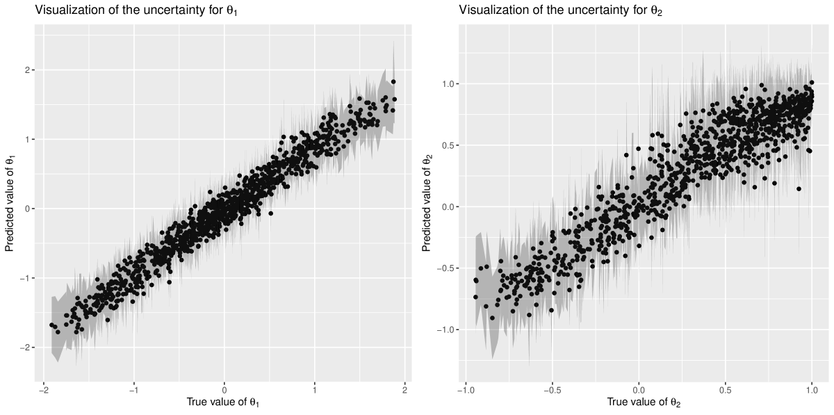
Figure 1: Moving Average 2 example: predicted parameters $\widehat{\theta_{1}}$ and $\widehat{\theta_{2}}$ estimated by the ABCD-conformal against the true values for the 1000 test samples, and confidence sets obtained by the conformal procedure (in gray intervals, for the epistemic uncertainty).

4.2 Two-dimensional Gaussian random field

4.2.1 The model

We study stationary isotropic Gaussian random fields on the domain $[0,5]\times[0,5]$ with a regular grid of size 100$\times$100, with exponential covariance functions [Wood and Chan,, 1994]. This covariance between two points $z_{1}$ and $z_{2}$ is given by:

$$C(z_{1},z_{2})=\exp\Big{(}\Big{|}\Big{|}\frac{z_{1}-z_{2}}{\theta}\Big{|}\Big{|}^{2}\Big{)},$$

with $\theta$ the range (or scale) parameter, which is the unknown parameter. We assume that the prior distribution on $\theta$ is the uniform distribution between 0 and 1.

4.2.2 Algorithm parametrization

Number of used samples are resumed in Table 1. Concerning the standard ABC and the ABC-RF, we use two summary statistics: the Moran’s $I$ statistics from lag 1 to 5 (that is the Moran’s correlogram from lags 1 to 5), and the semi-variogram up to a distance of 20 (15 values kept per variogram) (see Cliff and Ord, [1981] for these notions). We assume the spatial weights matrix to be row-standardised, and the neighbors of a pixel being the 4-nearest pixels. As all Gaussian fields are simulated on the same grid, the variograms of the different fields are calculated at exactly the same distances, so they are comparable. For the standard ABC, the distance used to compare two Gaussian random fields is the sum of the quadratic distance between their Moran’s correlograms and of the quadratic distance between their semi-variograms.

Concerning the architectures of neural networks for ABC-CNN and ABC-Dropout, we used 3 convolutional layers having 32, 64 and 64 neurons and the relu activation function, followed by 2 dense layers having both 64 neurons and the relu activation function. The raw samples given as inputs of the neural networks are the 2D Gaussian random fields, and the associated outputs are the estimations of the parameter $\theta$.

4.2.3 Results

All indicators detailed in the beginning of Section  4 are presented in Table 3. Figure 2 shows the predicted parameters $\widehat{\theta}$ estimated by the ABCD-conformal method against the true values for the 100 test samples, and using gray intervals.

	Standard	ABC-CNN	ABC-RF	ABCD-conformal	ABCD-conformal
	ABC			overall	epistemic
NMAE	0.0436	0.0223	0.0154	0.0303	0.0303
$sd(|\theta-\widehat{\theta}|)$	0.0229	0.0106	0.0077	0.0141	0.0141
coverage confidence sets $\theta$	100$\%$	88$\%$	99$\%$	93$\%$	95$\%$
mean length confidence sets $\theta$	0.1313	0.0307	0.0414	0.0684	0.0718

Table 3: Comparison of standard ABC, ABC-CNN, ABC-RF and ABCD-conformal on the two-dimensional Gaussian random field 2 example. These indicators are computed on a test set of size $10^{2}$.

In Table 3, we see that on this example, ABC-RF outperforms the others methods, with the smallest NMAE and $sd(|\theta-\widehat{\theta}|)$, while having a very good coverage, 99%, which is better than the expected coverage of 95%. The standard ABC and ABC-CNN do not give satisfactory results. Indeed, while having a coverage of 100%, the standard ABC has the largest NMAE and $sd(|\theta-\widehat{\theta}|)$, and the good coverage is due to too large . Concerning the ABC-CNN, like in the previous example, the NMAE, $sd(|\theta-\widehat{\theta}|)$ and the mean lengths of the confidence sets are quite small, but it is counterbalanced by a too small coverage (88%). Finally, the results given by the ABCD-conformal approach are sharp, with coverages of exactly 95% (for the epistimic uncertainty). The overall and the epistemic uncertainty give quite similar results in the conformal procedure.

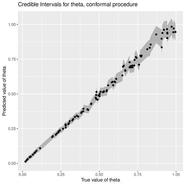
Figure 2: Predicted parameters $\widehat{\theta}$ estimated by the ABCD-conformal against the true values for the 100 test samples, and (in gray intervals, for the overall uncertainty).

To sum up, the ABC-RF is efficient here on all criteria. ABCD-Conformal and ABC-CNN give good predictions, but ABCD-Conformal is much better on . Standard ABC is unsatisfactory on all criteria.

4.3 Lokta-Volterra model

4.3.1 The model

The Lokta-Volterra model describes the dynamics of biological systems in which two species interact, one as a predator and the other as a prey. Here we consider a stochastic Markov jump process version of this model with state $(X_{1},X_{2})\in\mathbb{Z}^{2}$ representing prey and predator population sizes, and three parameters $c_{1},c_{2}$ and $c_{3}$. Three transitions are possible, with hazard rates $c_{1}X_{1}$, $c_{2}X_{1}X_{2}$ and $c_{3}X_{2}$ respectively:

$$(X_{1},X_{2}) \overset{c_{1}X_{1}}{\longrightarrow}(X_{1}+1,X_{2})\textrm{\qquad(prey growth)}$$

$$(X_{1},X_{2}) \overset{c_{2}X_{1}X_{2}}{\longrightarrow}(X_{1}-1,X_{2}+1)\textrm{\qquad(predation interaction)}$$

$$(X_{1},X_{2}) \overset{c_{3}X_{2}}{\longrightarrow}(X_{1},X_{2}-1)\textrm{\qquad(predator death)}$$

The estimation of the parameters of this Lokta Volterra model has been studied by several authors in an ABC framework, see for instance Prangle, [2017]. The initial conditions are $X_{1}(0)=50$ and $X_{2}(0)=100$ and a dataset corresponds to observations of state $(X_{1},X_{2})$ at times $0,2,4,\ldots,36$. As usual, all simulations with an extinction of either the preys or the predators were discarded : we are interested in the conditional law of survival. The prior distributions are independent uniforms $\mathcal{U}[-6,2]$ for the transformed parameters $\log(c_{1}),\log(c_{2})$ and $\log(c_{3})$.

We are interested here in the estimation of $\theta=(c_{1},c_{2},c_{3})$.

4.3.2 Algorithm parametrization

Number of used samples are resumed in Table 1. The Gillespie’s stochastic simulation algorithm is used to generate all the samples, using the Explicit tau-leap method from the package GillespieSSA2 [Cannoodt et al.,, 2021]. To improve performances of the algorithm, once simulations have been done, we used standardised versions of the parameters. The goal is then to obtain posterior estimates of the tri-dimensional vector of normalized parameters $(c_{1},c_{2},c_{3})$, from an observed sample consisting of two time series of sizes 19.

Concerning the standard ABC, there is no obvious summary statistics. Instead, the distance function $d\Big{(}(x_{1},x_{2}),(x_{1d},x_{2d})\Big{)}$ between a sample from the test set $\big{(}\{x_{1d}[i],x_{2d}[i]\},i=1,\ldots,19\big{)}$ and a sample from the training set $\big{(}\{x_{1}[i],x_{2}[i]\},i=1,\ldots,19\big{)}$ , is given by the sum of squared differences:

$$d\Big{(}(x_{1},x_{2}),(x_{1d},x_{2d})\Big{)}=\sum_{i=1}^{19}\Big{(}\big{(}x_{1}[i]-x_{1d}[i]\big{)}^{2}+\big{(}x_{2}[i]-x_{2d}[i]\big{)}^{2}\Big{)}$$

Concerning ABC-CNN, the distance function between a sample from the test set and a sample from the training set is the quadratic distances between the parameters predicted by the CNN for the test sample, and the true parameters used to simulate the training sample.

The architectures used for the neural networks are the same for the ABC-CNN and the ABCD-conformal: 3 convolutional 1D layers with 128 neurons and a kernel size of 2, followed by max-pooling for the first two layers, and by a flatten layer for the third one. Then, 3 dense layers of 100 neurons. Each of the layers use the tanh activation function. The raw samples consisting of two time series of lengths 19 are the inputs of the neural networks, and the outputs are the tri-dimensional associated vectors of parameters $(c_{1},c_{2},c_{3})$.

4.3.3 Results

All indicators detailed in the beginning of Section  4 are presented in Table 4. Figure 3 shows the predicted normalized parameters and associated confidence sets obtained with standard ABC, ABC-CNN and ABCD-conformal methods respectively for the 1000 test samples, and associated confidence sets.

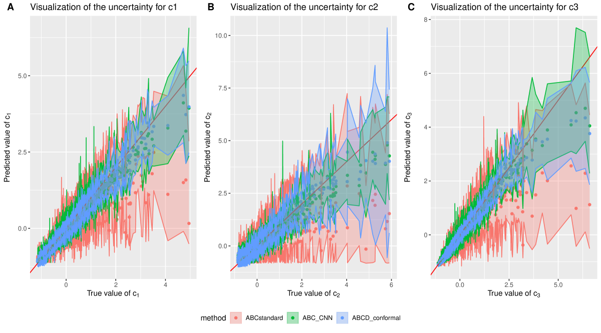
Figure 3: Lokta Volterra example: predicted normalized parameters $\widehat{c_{1}}$, $\widehat{c_{2}}$ and $\widehat{c_{3}}$ estimated by the standard ABC, the ABC-CNN and the ABCD-conformal methods, against the true values for the 1000 test samples. In gray are represented, for the overall uncertainty.

	Standard ABC	ABC-CNN	ABCD-conformal	ABCD-conformal
			overall	epistemic
$NMAE_{1}$	0.2647	0.1516	0.1294	0.1294
$NMAE_{2}$	0.3974	0.2421	0.1966	0.1966
$NMAE_{2}$	0.2770	0.1400	0.1206	0.1206
$sd(|c_{1}-\widehat{c_{1}}|)$	0.3735	0.1319	0.1106	0.1106
$sd(|c_{2}-\widehat{c_{2}}|)$	0.4865	0.1940	0.1714	0.1714
$sd(|c_{3}-\widehat{c_{3}}|)$	0.4368	0.1485	0.1534	0.1534
mean length confidence sets $c_{1}$	0.999	0.6847	0.4699	0.4956
mean length confidence sets $c_{2}$	1.447	0.8447	0.7671	1.0184
mean length confidence sets $c_{3}$	1.012	0.6218	0.3807	0.4176
coverage confidence sets $c_{1}$	$91.7\%$	$91.7\%$	$92.1\%$	$91.0\%$
coverage confidence sets $c_{2}$	$94.2\%$	$93.3\%$	$95.6\%$	$96.3\%$
coverage confidence sets $c_{3}$	$95.9\%$	$97.2\%$	$91.9\%$	$90.1\%$

Table 4: Lokta Volterra example: comparison of standard ABC, ABC-CNN and ABCD-conformal (using overall or epistemic uncertainty as uncertainty heuristic for the conformal procedure). These indicators are computed on a test set of size $10^{3}$.

We can see in table 4 that ABCD-conformal outperforms standard ABC and obtains quite better results than ABC-CNN, when looking at NMAE and standard deviations of the absolute errors. Predictions of ABC-CNN and ABCD-conformal are better than those of the standard ABC, thanks to the power of CNN, and because we do not have relevant summary statistics for the standard ABC. Thanks to Dropout, the predictions are even better for ABCD-conformal than for ABC-CNN.
The confidence sets coverages appear similar for the three methods. But the mean lengths of confidence sets are different depending on the method and on the parameter. Using this criterion, ABCD-conformal is the best, followed by ABC-CNN then by standard ABC, for the three parameters. In this example, there is also an impact of the heuristic uncertainty measure used for the conformal procedure: the overall variance gives slightly better results than the epistemic variance for $c_{1}$ and $c_{3}$, and this impact is bigger for $c_{2}$.
We also note that the lengths of the confidence sets are quite different depending on the regions of the normalized parameters, for all methods. To understand in more detail what’s happening, we compute the mean lengths of confidence sets, as well as coverages, for different regions of the normalized parameter $c_{3}$. The results are summarized in Table 5, and similar results were obtained for the two other parameters $c_{1}$ and $c_{2}$.
We can understand that the performances of the different methods can vary a lot depending on the region of the parameter. The coverages on the whole domain are quite different from the coverages on some specific regions. For instance, the coverage of standard ABC (resp. ABCD conformal) on the whole domain is $95.9\%$ (resp $91.9\%$), while it is only $53.3\%$ for $c_{3}>3$ (resp $80.0\%$). Hence, even if in theory ABCD-conformal gives marginal coverage and standard ABC gives conditional coverages, in this example standard ABC also does not give similar coverages depending on the region.

		Standard ABC	ABC-CNN	ABCD-conformal overall
$c_{3}<1$	mean length confidence sets	0.7271	0.4970	0.2808
860 datasets	coverage	$96.3\%$	$96.7\%$	$91.9\%$
$1<c_{3}<3$	mean length confidence sets	2.5856	1.2039	0.8366
125 datasets	coverage	$98.4\%$	$100\%$	$93.6\%$
$3<c_{3}$	mean length confidence sets	4.2436	2.9231	2.3087
15 datasets	coverage	$53.3\%$	$100\%$	$80.0\%$

Table 5: Lokta Volterra example: comparison of standard ABC, ABC-CNN and ABCD-conformal (using overall uncertainty as uncertainty heuristic for the conformal procedure), in different regions for the normalized parameter $c_{3}$. These indicators are computed on a test set of size $10^{3}$.

To sum up, ABCD-Conformal is better than the other methods in this example, with better predicitons and narrower confidences sets, for similar coverages. We noted that the coverages are quite different in different regions of the parameters, illustrating the marginality of the coverage, but this is the case for ALL methods.

5 Discussion

In this article we propose a new ABC method that combines several approaches: the ABC framework, Neural Networks with Monte Carlo Dropout and a conformal procedure. This method is free of any summary statistic, distance or tolerance threshold. It is able to deal with multidimensional parameters, and gives exact non-asymptotic confidences sets.

In practice, this method is computationally efficient, and obtains good results. We test the method on three examples and compare its performances with other approaches: standard ABC, ABC-RF and ABC-CNN. We observe that depending on the problem at hand, standard ABC or ABC-RF can have slightly better accuracy. However, we also see in the Lokta-Volterra example that ABCD-conformal can also outperforms them. Regarding ABC-CNN, on all examples it never outperfoms the ABCD-conformal, either because of bad coverages of confidence sets, or because of larger mean lengths of these intervals. In contrast with the other methods, ABCD-conformal is the only one with guaranteed coverages for confidence sets. A big advantage of ABCD-conformal in our practice, is that it always gives both a good estimation accuracy and a good marginal frequentist coverage, which is not always the case for the other methods. It is an alternative to other methods when there is no obvious summary statistic. Moreover, the computing time is comparable with ABC-CNN and ABC-RF. The choice of the summary statistics is replaced by the choice of a network architecture. This choice can be guided by common Deep Learning architectures (imaging, time series, …) and the massive associated literature. A drawback of our proposed method is that the coverage of the confidence sets is valid marginally, and not conditionally to some values of the parameters of interest. Indeed, on the Lokta-Volterra example we have seen that the performances of the methods can vary a lot depending on the region of the parameter. However, note that this was the case for ALL methods studied.
For a more detailed comparison between the four ABC methods used, the reader can refer to Appendix B.

The ABCD-conformal algorithm proposed is promising. However, several improvements and modifications could be considered mostly at the level of the uncertainty proxy outputted by the neural network and the conformal procedure.

Concerning the neural network, we can imagine to use the Dropconnect technique instead of Dropout. These two techniques prevent "co-adaptation" of units in a neural network. Dropout randomly drops hidden nodes, and Dropconnect drops connections (but all nodes can remain partially active). Dropconnect is a generalization of Dropout since there are more possible connections than nodes in a neural network. Another possibility to be explored, could be to use ensembles of neural networks (or deep ensembles) to obtain a random estimation of the parameter of interest and associated uncertainties, see Lakshminarayanan et al., [2017]. As explained by Srivastava et al., 2014c , Dropout can even be interpreted as ensemble model combination.

Regarding the conformal procedure, in this article we focused on conformalizing a scalar uncertainty estimate, because the parameter of interest $\theta$ is a vector of scalars. But we can also use conformalized quantile regression (see Angelopoulos and Bates, [2023] for a presentation of this procedure). Finally, in the method proposed, we have considered a split conformal procedure. This is computationally attractive, as the model needs to be fitted only one time. But it requires to have a calibration set, in addition to the training and validation ones (even if in general this set is quite small compared to the training set). Full conformal procedure could avoid these extra simulations, at the cost of many more model fits, see Angelopoulos and Bates, [2023]. Hence, choosing between split or full conformal procedure could depend on the problem at hand.

Appendix A Pseudo-codes for ABC-CNN and ABC-RF and some comments

A.1 ABC-CNN

1

Input : A Bayesian parametric model $\{f(\cdot\mid\theta),\pi\}$, a data sample $\mathbf{x}$, integers $N_{\text{train}}$ and $N_{val}$ representing sizes of training, and validation sets, a (pseudo)-distance $d$ between two samples, and a tolerance threshold $\alpha\in(0,1]$.

2

Output : A set $\theta_{1},\ldots,\theta_{[N_{\text{train}}\alpha]}$ whose distribution is approximately $\pi(\theta\mid\mathbf{x})$

3

4Generation of a reference table (training dataset) :

5 for $j\leftarrow 1$ to $N_{\text{train}}$ do

6       Draw $\theta_{j}\sim\pi$;

7      

8      Draw synthetic sample $\mathbf{x}_{j}=(x_{1,j},\ldots,x_{d,j})^{\top}$ from the model $f(\cdot\mid\theta_{j})$;

9      

10 end for

11

12Generation of a validation dataset :

13 for $j\leftarrow 1$ to $N_{val}$ do

14       Draw $\theta_{j}\sim\pi$;

15      

16      Draw synthetic sample $\mathbf{x}_{j}=(x_{1,j},\ldots,x_{d,j})^{\top}$ from the model $f(\cdot\mid\theta_{j})$;

17      

18 end for

19

20Train a CNN on the reference table: inputs of the CNN are the $\left\{\mathbf{x}_{j},j=1,\ldots,N_{\text{train}}\right\}$, and the outputs are the $\left\{\theta_{j},j=1,\ldots,N_{\text{train}}\right\}$. The validation set is used to choose the architecture of the CNN.

21Summary statistics and distances :

22 for $j\leftarrow 1$ to $N_{\text{train}}$ do

23       $\mathbf{x}_{j}$ is given as input to the trained CNN $\eta_{\mathrm{CNN}}$ to obtain an estimate of the posterior expected value for $\theta_{j}=\eta_{\mathrm{CNN}}(\mathbf{x}_{j})$. ;

24      

25      Compute the distance $d_{j}=d(\eta_{\mathrm{{CNN}}}(\mathbf{x}),\eta_{\mathrm{{CNN}}}(\mathbf{x}_{j}))$ ;

26 end for

27

28Order these distances, i.e., $d_{(1)}<d_{(2)}<\cdots<d_{(N_{\text{train}})}$;

29

Keep the $\theta_{j}$ corresponding to the $\lfloor N_{\text{train}}\alpha\rfloor$ smallest distances.

Algorithm 3 Pseudo code for CNN as Summary Statistics for ABC [Akesson et al.,, 2022]

The approach of Akesson et al., [2022] is simply a small modification of the standard ABC, where CNNs are used to estimate the posterior mean of a parameter, which is then used as a summary statistic. The line 8 of the standard ABC algorithm (Algorithm 1) to compute summary statistics, is replaced by the prediction of a CNN trained on the reference table, see lines 11, 14 and 15 of Algorithm 3. The output of the algorithm is similar to the one of the standard ABC: for a given data sample $\mathbf{x}$ and a tolerance threshold, we hope that the parameters $\theta$ accepted during the process are approximately distributed from the posterior distribution $\pi(\theta\mid\mathbf{x})$. Hence to have asymptotic consistency and valid frequentist coverages, the same kind of conditions are needed than for Algorithm 1. But it’s harder to check these conditions for ABC-CNN than for standard ABC, because the summary statistic used in the ABC-CNN is the output of a CNN which is a "black-box". It is therefore practically impossible to verify anything about this summary statistic.

Although, there are some important differences that are worth highlighting between the two methods. The main and most important one is that it is not necessary to give summary statistics, thanks to the use of a CNN which automatically generates a relevant one. However, a distance $d$ for comparing two data samples and a tolerance threshold $\alpha$ are still required. In practice, this distance is often simpler to determine in the case of ABC-CNN than in the case of standard ABC, because comparing two parameters is often simpler than comparing two sets of summary statistics, which can be numerous and very diverse. Theoretically, as explained by Frazier et al., [2018], for a fixed choice of summaries, the two-stage procedure advocated by Fearnhead and Prangle, [2012] and used by Akesson et al., [2022], will not reduce the asymptotic variance over a point estimate of a parameter produced via Algorithm 1. However, this two-stage procedure does reduce the Monte Carlo error inherent in estimating the approximate posterior distribution $\pi_{\alpha,d}(.\mid\eta(\mathbf{x}))$ by reducing the dimension of the statistics on which the matching in approximate Bayesian computation is based. Using this approach, we can hope to have a smaller global error of approximation of the true posterior, compared to standard ABC.

Moreover, a CNN can deal with different types of data, in particular high dimensional and complex data, like temporal or spatial data. Parameters can be easily estimated from these complex data by a CNN, while it can be difficult to find appropriate summary statistics to be used in a classical ABC.

Another difference with the standard ABC is that a validation dataset should be generated, to be used to choose the network architecture, as usual for neural networks. This dataset is generally much smaller in size than the reference table used as a training set. Therefore, it generally adds little computation time compared with the effort required to generate the reference table. This lost computation time can be recovered, and time can even be saved, in the classical ABC step. Indeed, in this step, the sample of interest $\mathbf{x}$ for which we want to approximate the posterior $\pi(\theta\mid\mathbf{x})$ should be compared with all the samples in the reference table (lines 9 of Algorithm 1 and 15 of Algorithm 3). This comparison can be time consuming, depending on the distance used between summary statistics and the size of the reference table. If there are many summary statistics to be used by the standard ABC, the ABC-CNN which uses only one summary statistic, will be much faster. The larger the reference table, the greater the difference. This is why, in many cases, ABC-CNN will often be faster than standard ABC, despite the generation of a validation set. However, we can not generalise and it clearly depends on the problem at hand.

A.2 ABC-RF

Raynal et al., [2018] who propose to conduct likelihood-free Bayesian inferences about parameters with no prior selection of the relevant components of summary statistics and bypassing the derivation of the associated tolerance threshold. The approach relies on the random forest (RF) methodology of Breiman, [2001] applied in a regression setting.

1

Input : A Bayesian parametric model $\{f(\cdot\mid\theta),\pi\}$, a data sample $\mathbf{x}$, $N_{\text{train}}$ the size of the training set, summary statistics $\eta:\mathbb{R}^{d}\to\mathbb{R}^{l}$.

2

Output : For $T(\theta)$ a scalar transform of $\theta$, approximations of the posterior expected value $\psi_{\eta}(\mathbf{x})=\mathbb{E}_{\pi}[T(\theta)\mid\eta(\mathbf{x})]$, the posterior variance $\mathbb{V}_{\pi}[T(\theta)\mid\eta(\mathbf{x})]$, and posterior quantiles.

3

4Generation of a reference table :

5 for $j\leftarrow 1$ to $N_{\text{train}}$ do

6       Draw $\theta_{j}\sim\pi$;

7      

8      Draw synthetic sample $\mathbf{x}_{j}=(x_{1,j},\ldots,x_{d,j})^{\top}$ from the model $f(\cdot\mid\theta_{j})$ 

9 end for

10

11Summary statistics :

12 for $j\leftarrow 1$ to $N_{\text{train}}$ do

13       Compute the vector of summary statistics $\eta(\mathbf{x}_{j})$ 

14 end for

15

16Train a random forest: inputs of the random forest are the $\left\{\eta(\mathbf{x}_{j}),j=1,\ldots,N_{\text{train}}\right\}$, and the outputs are the $\left\{T(\theta_{j}),j=1,\ldots,N_{\text{train}}\right\}$.

Approximate $\psi_{\eta}(\mathbf{x})$: give $\eta(x)$ as input of the trained random forest: the output of the RF allows to obtain easily approximations of $\psi_{\eta}(\mathbf{x})=\mathbb{E}_{\pi}[T(\theta)\mid\eta(\mathbf{x})]$, $\mathbb{V}_{\pi}[T(\theta)\mid\eta(\mathbf{x})]$ and of posterior quantiles (hence credible intervals).

Algorithm 4 Pseudo code for an Approximate Bayesian Computation - Random Forest sampler

This algorithm automatises the inclusion of summary statistics and do not need the definition of a distance or the choice of a tolerance threshold. It appears mostly insensitive to the presence of non relevant summary statistics. It can then deal with a large number of summary statistics, by-passing any form of pre-selection. However, it is mandatory that relevant ones are present in the initial pool of summary statistics to be considered. To obtain posterior quantiles and then credible intervals, this ABC-RF method uses quantile regression forests to approximate the posterior cumulative distribution function of $T(\theta)$ given $\eta(\mathbf{x})$, $F(T(\theta)\mid\eta(\mathbf{x}))$. The asymptotic consistency of this approach has been established by Meinshausen, [2006], under some conditions. In particular, $F(T(\theta)\mid\eta(\mathbf{x}))$ should be Lipschitz continuous and strictly monotonously increasing in $T(\theta)$. Such conditions are practically unverifiable in an ABC framework where the likelihood is unknown or intractable.

In practice, Raynal et al., [2018] showed on several examples that the approximations of posterior expectations obtained by ABC-RF were quite accurate, while posterior variances were slightly overestimated, and confidence sets slightly conservative (larger than the exact ones).

Appendix B Detailed comparison of the four ABC methods used in the examples

Below the four methods used (standard ABC, ABC-CNN, ANC-RF and ABCD-conformal) are compared in details on different points, with a practical point of view. Table 4 summarizes these reflexions.

Output of the algorithm
First, one big difference between these methods is what is obtained from the algorithm: for standard ABC and ABC-CNN an approximation of the whole posterior distribution of the parameter of interest is obtained. Concerning ABC-RF and ABCD-conformal, these methods focus on the approximation of transforms of interest of the posterior, like posterior mean, posterior variance or posterior quantiles for instance. It is rather common that only transforms of the posterior are of interest for practionners, and in this case all four methods can be used. But if the whole posterior would be studied, ABC-RF and ABCD-conformal will not be adapted. Note that to obtain a good approximation of the whole posterior, in general more simulations are required than for simply estimating transforms of the posterior.

Need of relevant summary statistic
Standard ABC need summary statistics to be able to compare simulations and observed data. Sometimes obvious relevant statistics exist (like in the MA2 example for instance), and the best is to have exhaustive statistics. But most of the time, it is not easy to find such relevant statistics and it is a serious bottleneck when performing inference on complex and high-dimensional problems. As explained in section 2.1, it is preferable to have a small number of summary statistics to avoid the burden of multidimensionality, and these statistics should be sufficiently informative [Fearnhead and Prangle,, 2012]. Concerning ABC-RF, it enables to automatise the inclusion of summary statistics in an ABC algorithm. But it is necessary to have a set of statistics from which to select relevant ones: relevant statistics should be in the set, and this is a limitation. ABC-CNN and ANCD-conformal do not need any summary statistic, which is an advantage as the choice of these summaries have been proven to be crucial to obtaining good results.

Need for a distance
A distance to compare simulations and observed data is needed for standard ABC. This distance depends on the summary statistics used and on the problem at hand. Specific distances can be used for genetics problem for instance. In general, a good knowledge of the problem in question and discussions with experts are necessary to define a relevant distance. In case of low-dimensional statistics, relevant distances are generally faster to compute. But in case of high-dimensional statistics, they can be quite long to compute. This is the case of the Lokta-Volterra example: we did not really used summary statistics as datasets and simulations were directly compared using an euclidian distance. But as the dataset was of dimension fourty (two series of twenty times), it was computationaly demanding: the standard ABC was the method which took more computing time. Concerning the ABC-CNN algorithm, a summary statistic is obtained through the network, and the distance to be used is in general quite simple and fast to be computed. Of course computing time increases with the dimension of the parameters of interest, but in our examples with a maximum parameter dimension of three, it was very fast. ABC-RF and ABCD-conformal do not need any distance, which can avoid a tricky choice and can save computational time.

Need for a tolerance threshold
For standard ABC and ABC-CNN, a tolerance threshold is also needed and its choice affects the degree of approximation obtained for the whole distribution. Usually, for practical reasons, quantile-based acceptance thresholds are used (quantiles of the distances between the observed data set and simulations in the training set). ABC-RF and ABCD-conformal do not need a tolerance threshold, as they do not use a distance.

Dealing with multidimensional parameters
Concerning the parameter of interest, the ABC-RF method can estimate only uni-dimensional transforms of interest, usually a projection on a given coordinate of the parameter. In the discussion of their article, Raynal et al., [2018] explained that their attempts to deal with multidimensional parameters were so far unfruitful. The standard ABC can deal with multidimensional parameter, but it suffers from the burden of multidimensionality, as summary statistics and distances are more difficult to define, and take more time to be computed in high dimension. ABC-CNN, despite having a standard ABC step in the algorithm, suffers less from this burden, as the summary statistic obtained through the CNN is of the same dimension than the parameter of interest (no more than dimension three in our exmaples). Concerning ABCD-conformal, multidimensionality is not a problem, as the computing time for the CNN with droupout and the conformal procedure does not really increases with the dimension (at least on the examples studied, with a maximum dimension of three).

Choose network or random forest architecture
ABC-CNN and ABCD-conformal are based on neural networks. Hence the architecture of the networks to be used should be chosen: mainly the number of layers, the type of layer, the number of neurons in a layers, the size of the kernel for convolutional layers, and the activation functions. For the Dropout rate, we do not need to choose it when using the concrete Dropout approach of Gal et al., [2017]. In practice, for the examples studied, we did not spend too much time to choose the architecture, as it is quite fast to train different networks and to compare them on the validation set. The most influential parameters for us in our examples were the type of layers (convolutional or dense), and the activation functions. Similarly, to use ABC-RF some parameters should be chosen for the random forest, mainly the number of trees, the minimum node size and the proportion of summary statistics sampled at each split. For this method also, we did not encounter difficulties to set these parameters, standard values making the job on our example.

Needed datasets
Standard ABC and ABC-RF need a training set of simulations, to be compared with the observed data. ABC-CNN also needs a validation set, which is used to choose the network architecture. Concerning the ABCD-conformal, it also needs a calibration set for the conformal procedure. This calibration set is usually of size 500 or 1000 depending on the accuracy we want for the marginal coverage [Angelopoulos and Bates,, 2023]. Therefore, more simulations are needed for ABC-CNN than for standard ABC and ABC-RF, and even more for ABCD-conformal. However, the sizes of the validation and of the calibration sets are generally quite smaller than the size of the training set, and the increase in simulation time is small compared to what is required for the training set. This time can often be recovered in other steps of the algorithm.

Theoretical justification of the methods
In this article, we are particularly interested by the estimation of parameters of interest, with associated confidence sets. The question of the frequentist coverage of the obtained intervals matters, as the intervals represent our uncertainty of our estimation. We then compared the frequentist coverage of the obtained intervals for the different methods, on three examples, and we studied the bibliography for the theoretical justification of all these methods.

As detailed in section 2.1, Frazier et al., [2018] studied asymptotic properties of standard ABC and gave conditions under which Bayesian confidence sets have valid frequentist coverage levels. Hence, in theory and asymptotically, under some regularity conditions, standard ABC and ABC-CNN methods enable posterior concentration and the probability matching criterion. But these conditions can not be verified in general, and this restricts the use and validity of these methods.

Concerning the ABC-RF, as said in section 2.2.2, it is based on quantile regression forests whose asymptotic consistency has been proved by Meinshausen, [2006] under some conditions. But these conditions are practically unverifiable in an ABC framework.

On the opposite, the ABCD-conformal method guarantees a non-asymptotic marginal frequentist coverage, without any distributional or model assumption. The test points should solely come from the same distribution as the calibration points. Only the efficiency of the conformal procedure is in question, as the lengths of the confidence sets will depend on the quality of the uncertainty measure used in the procedure. This guaranteed coverage is a great advantage compared to the other methods. However, this coverage is guaranteed marginally, and not conditionally. Nevertheless, some metrics can be computed to check how close we are to conditional marginality, see Angelopoulos and Bates, [2023].

Benefits of using concrete Dropout
Apart from the fact that epistemic and aleatoric uncertainties are used to obtain credibility intervals during the conformal procedure, their values themselves and the distinction between these uncertainties are interesting for effective exploration of the uncertainty: which part can be attributed to the model or to the noise in the data, in which circumstances?

Est ce que dans le tableau je rajoute un point "Simplicity of method coding"? Ou bien j’en parle juste dans le texte? Car la simplicité d’utilisation dépend de la complexité de la méthode en elle-même, mais aussi du fait de devoir trouver/calculer des summary stats pour les méthodes ABC standard et ABC-CNN. En gros ABC-CNN et ABCD-conformal peuvent paraitre plus complexes, mais en même temps elles ne nécessitent aucun traitement préalable des données. Donc dur de mettre un smiley généralisant dans le tableau.

Point of comparison	Standard ABC	ABC-CNN	ABC-RF	ABCD-conformal
Approx. of the whole posterior	whole	whole	transforms	transforms
or of transforms of interest	posterior	posterior	of interest	of interest
No need of relevant
summary stat	✗	✓	✗	✓
No need of a
distance	✗	✓	✓	✓
No need of a
tolerance threshold	✗	✗	✓	✓
Deal with multidimensional
parameters	✓	✓	✗	✓
No need to choose network or
random forest architecture	✓	✗	✗	✗
Datasets needed	1: training	2: training,	1: training	3: training,
		validation		validation,
				calibration
Justification of	asymptotic	asymptotic	asymptotic	non asymptotic
the method,	under conditions	conditions too dif-	conditions too dif-	no condition
guarantees		ficult to check	ficult to check
Adapted for different types	difficult		difficult
of data and high-dim data	✗	✓	✗	✓
Computing time	difficult to compare, it depends on examples.

Table 6: Summary table comparing the four methods: standard ABC, ABC-CNN, ABC-RF and ABCD-conformal.

References

- Akesson et al., [2022] Akesson, M., Singh, P., Wrede, F., and Hellander, A. (2022). Convolutional neural networks as summary statistics for approximate bayesian computation. IEEE/ACM Transactions on Computational Biology and Bioinformatics, 19(06):1–1.
- Angelopoulos and Bates, [2023] Angelopoulos, A. N. and Bates, S. (2023). Conformal prediction: A gentle introduction. Foundations and Trends® in Machine Learning, 16(4):494–591.
- Baragatti and Pudlo, [2014] Baragatti, M. and Pudlo, P. (2014). An overview on approximate bayesian computation*. ESAIM: Proc., 44:291–299.
- Besag, [1974] Besag, J. (1974). Spatial interactions and the statistical analysis of lattice systems. Journal of the Royal Statistical Society. Series B. Statistical methodology, 148:1–36.
- Blum et al., [2012] Blum, M., Nunes, M., Prangle, D., and Sisson, S. (2012). A comparative review of dimension reduction methods in approximate bayesian computation. stat sci 28: 189-208. Statistical Science, 28.
- Boston et al., [2022] Boston, T., Dijk, A., Larraondo, P., and Thackway, R. (2022). Comparing cnns and random forests for landsat image segmentation trained on a large proxy land cover dataset. Remote Sensing, 14:3396.
- Breiman, [2001] Breiman, L. (2001). Random forests. Machine Learning, 45:5–32.
- Cannoodt et al., [2021] Cannoodt, R., Saelens, W., Deconinck, L., and Saeys, Y. (2021). Spearheading future omics analyses using dyngen, a multi-modal simulator of single cells. Nature Communications.
- Cliff and Ord, [1981] Cliff, A. D. and Ord, J. K. (1981). Spatial processes: models and applications. Pion Ltd, London, UK.
- Courville et al., [2016] Courville, A., Goodfellow, I., and Bengio, Y. (2016). Deep Learning. Adaptive computation and machine learning series. MIT Press.
- Dantas et al., [2023] Dantas, C. F., Drumond, T. F., Marcos, D., and Ienco, D. (2023). Counterfactual explanations for remote sensing time series data: An application to land cover classification. In Joint European Conference on Machine Learning and Knowledge Discovery in Databases, pages 20–36. Springer.
- Datta et al., [2000] Datta, G. S., Ghosh, M., Mukerjee, R., and Sweeting, T. J. (2000). Bayesian prediction with approximate frequentist validity. The Annals of Statistics, 28(5):1414 – 1426.
- de Haan, [1984] de Haan, L. (1984). A spectral representation for max-stable processes. The Annals of Probability, 12(4):1194–1204.
- Dereich et al., [2013] Dereich, S., Scheutzow, M., and Schottstedt, R. (2013). Constructive quantization: Approximation by empirical measures. In Annales de l’IHP Probabilités et statistiques, volume 49, pages 1183–1203.
- Fearnhead and Prangle, [2012] Fearnhead, P. and Prangle, D. (2012). Constructing summary statistics for approximate bayesian computation: semi-automatic approximate bayesian computation. Journal of the Royal Statistical Society: Series B (Statistical Methodology), 74(3):419–474.
- Filos et al., [2020] Filos, A., Tigkas, P., McAllister, R., Rhinehart, N., Levine, S., and Gal, Y. (2020). Can autonomous vehicles identify, recover from, and adapt to distribution shifts? In International Conference on Machine Learning, pages 3145–3153. PMLR.
- Folgoc et al., [2021] Folgoc, L. L., Baltatzis, V., Desai, S., Devaraj, A., Ellis, S., Manzanera, O. E. M., Nair, A., Qiu, H., Schnabel, J., and Glocker, B. (2021). Is mc dropout bayesian? arXiv preprint arXiv:2110.04286.
- Fournier and Guillin, [2015] Fournier, N. and Guillin, A. (2015). On the rate of convergence in wasserstein distance of the empirical measure. Probability theory and related fields, 162(3):707–738.
- Frazier et al., [2018] Frazier, D. T., Martin, G. M., Robert, C. P., and Rousseau, J. (2018). Asymptotic properties of approximate Bayesian computation. Biometrika, 105(3):593–607.
- Gal, [2016] Gal, Y. (2016). Uncertainty in deep learning. PhD thesis, University of Cambridge.
- Gal and Ghahramani, [2016] Gal, Y. and Ghahramani, Z. (2016). Dropout as a bayesian approximation: Representing model uncertainty in deep learning. In international conference on machine learning, pages 1050–1059.
- Gal et al., [2017] Gal, Y., Hron, J., and Kendall, A. (2017). Concrete dropout. 31st Conference on Neural Information Processing System.
- Gobet et al., [2022] Gobet, E., Lerasle, M., and Métivier, D. (2022). Mean estimation for randomized quasi monte carlo method. Hal preprint hal-03631879v2.
- Grelaud et al., [2009] Grelaud, A., Marin, J.-M., Robert, C. P., Rodolphe, F., and Taly, J.-F. (2009). ABC likelihood-free methods for model choice in gibbs random fields. Bayesian Analysis, 4.
- Guéron, [2019] Guéron, A. (2019). Hands-On Machine Learning with Scikit-Learn, Keras, and TensorFlow, 2nd Edition. O’Reilly Media, Inc.
- Hinton et al., [2012] Hinton, G. E., Srivastava, N., Krizhevsky, A., Sutskever, I., and Salakhutdinov, R. (2012). Improving neural networks by preventing co-adaptation of feature detectors. CoRR, abs/1207.0580.
- Hoff, [2023] Hoff, P. (2023). Bayes-optimal prediction with frequentist coverage control. Bernoulli, 29(2):901 – 928.
- Izmailov et al., [2021] Izmailov, P., Vikram, S., Hoffman, M. D., and Wilson, A. G. G. (2021). What are bayesian neural network posteriors really like? In International conference on machine learning, pages 4629–4640. PMLR.
- Jiang et al., [2017] Jiang, B., Wu, T.-Y., Zheng, C., and Wong, W. H. (2017). Learning summary statistic for approximate bayesian computation via deep neural network. Statistica Sinica, 27:1595–1618.
- Jospin et al., [2022] Jospin, L. V., Laga, H., Boussaid, F., Buntine, W., and Bennamoun, M. (2022). Hands-On Bayesian Neural Networks—A Tutorial for Deep Learning Users. IEEE Computational Intelligence Magazine, 17(2):29–48.
- Joyce and Marjoram, [2008] Joyce, P. and Marjoram, P. (2008). Approximately sufficient statistics and bayesian computation. Statistical applications in genetics and molecular biology, 7:Article26.
- Kompa et al., [2021] Kompa, B., Snoek, J., and Beam, A. L. (2021). Empirical frequentist coverage of deep learning uncertainty quantification procedures. Entropy, 23(12).
- Lakshminarayanan et al., [2017] Lakshminarayanan, B., Pritzel, A., and Blundell, C. (2017). Simple and scalable predictive uncertainty estimation using deep ensembles. In Proceedings of the 31st International Conference on Neural Information Processing Systems, NIPS’17, page 6405–6416, Red Hook, NY, USA. Curran Associates Inc.
- LeCun et al., [1999] LeCun, Y., Haffner, P., Bottou, L., and Bengio, Y. (1999). Object Recognition with Gradient-Based Learning, pages 319–345. Springer Berlin Heidelberg, Berlin, Heidelberg.
- MacKay, [1992] MacKay, D. J. (1992). A practical bayesian framework for backpropagation networks. Neural computation, 4(3):448–472.
- Marin et al., [2012] Marin, J.-M., Pudlo, P., Robert, C. P., and Ryder, R. J. (2012). Approximate bayesian computational methods. Statistics and computing, 22(6):1167–1180.
- Marin and Robert, [2007] Marin, J.-M. and Robert, C. (2007). Bayesian Core: A Practical Approach to Computational Bayesian Statistics. Springer New York, NY.
- Marjoram et al., [2003] Marjoram, P., Molitor, J., Plagnol, V., and Tavaré, S. (2003). Markov chain Monte Carlo without likelihoods. Proceedings of the National Academy of Sciences of the USA, 100(26):15324–15328.
- McKinley et al., [2009] McKinley, T., Cook, A. R., and Deardon, R. (2009). Inference in epidemic models without likelihoods. The International Journal of Biostatistics, 5(1).
- Meinshausen, [2006] Meinshausen, N. (2006). Quantile regression forests. Journal of Machine Learning Research, 7(35):983–999.
- Messoudi et al., [2022] Messoudi, S., Destercke, S., and Rousseau, S. (2022). Ellipsoidal conformal inference for multi-target regression. In Conformal and Probabilistic Prediction with Applications, pages 294–306. PMLR.
- Neal, [2012] Neal, R. M. (2012). Bayesian learning for neural networks, volume 118. Springer Science & Business Media.
- Piccioni et al., [2022] Piccioni, F., Casenave, C., Baragatti, M., Cloez, B., and Vinçon-Leite, B. (2022). Calibration of a complex hydro-ecological model through approximate bayesian computation and random forest combined with sensitivity analysis. Ecological Informatics, 71:101764.
- Prangle, [2017] Prangle, D. (2017). Adapting the ABC Distance Function. Bayesian Analysis, 12(1):289 – 309.
- Pritchard et al., [1999] Pritchard, J., Seielstad, M., Perez-Lezaun, A., and Feldman, M. (1999). Population growth of human Y chromosomes: a study of Y chromosome microsatellites. Molecular Biology and Evolution, 16:1791–1798.
- Raynal et al., [2018] Raynal, L., Marin, J.-M., Pudlo, P., Ribatet, M., Robert, C. P., and Estoup, A. (2018). ABC random forests for Bayesian parameter inference. Bioinformatics, 35(10):1720–1728.
- Rousseau and Szabo, [2016] Rousseau, J. and Szabo, B. (2016). Asymptotic frequentist coverage properties of bayesian credible sets for sieve priors in general settings. Annals of Statistics, 48.
- Simola et al., [2021] Simola, U., Cisewski-Kehe, J., and Wolpert, R. L. (2021). Approximate bayesian computation for finite mixture models. Journal of Statistical Computation and Simulation, 91(6):1155–1174.
- Sisson et al., [2007] Sisson, S. A., Fan, Y., and Tanaka, M. M. (2007). Sequential monte carlo without likelihoods. Proceedings of the National Academy of Sciences, 104(6):1760–1765.
- [50] Srivastava, N., Hinton, G., Krizhevsky, A., Sutskever, I., and Salakhutdinov, R. (2014a). Dropout: a simple way to prevent neural networks from overfitting. The journal of machine learning research, 15(1):1929–1958.
- [51] Srivastava, N., Hinton, G., Krizhevsky, A., Sutskever, I., and Salakhutdinov, R. (2014b). Dropout: A simple way to prevent neural networks from overfitting. Journal of Machine Learning Research, 15(56):1929–1958.
- [52] Srivastava, N., Hinton, G., Krizhevsky, A., Sutskever, I., and Salakhutdinov, R. (2014c). Dropout: a simple way to prevent neural networks from overfitting. J. Mach. Learn. Res., 15(1):1929–1958.
- Vovk et al., [1999] Vovk, V., Gammerman, A., and Saunders, C. (1999). Machine-learning applications of algorithmic randomness. In Sixteenth International Conference on Machine Learning (ICML-1999) (01/01/99), pages 444–453.
- Wasserman, [2011] Wasserman, L. (2011). Frasian inference. Statistical Science, 26(3):322–325.
- Weed and Bach, [2019] Weed, J. and Bach, F. (2019). Sharp asymptotic and finite-sample rates of convergence of empirical measures in Wasserstein distance. Bernoulli, 25(4A):2620 – 2648.
- Wiqvist et al., [2019] Wiqvist, S., Mattei, P.-A., Picchini, U., and Frellsen, J. (2019). Partially exchangeable networks and architectures for learning summary statistics in approximate Bayesian computation. In Chaudhuri, K. and Salakhutdinov, R., editors, Proceedings of the 36th International Conference on Machine Learning, volume 97 of Proceedings of Machine Learning Research, pages 6798–6807. PMLR.
- Wood and Chan, [1994] Wood, A. T. A. and Chan, G. (1994). Simulation of stationary gaussian processes in [0, 1] d. Journal of Computational and Graphical Statistics, 3:409–432.
- Xu et al., [2019] Xu, F., Uszkoreit, H., Du, Y., Fan, W., Zhao, D., and Zhu, J. (2019). Explainable AI: A brief survey on history, research areas, approaches and challenges. In Tang, J., Kan, M.-Y., Zhao, D., Li, S., and Zan, H., editors, Natural Language Processing and Chinese Computing, pages 563–574, Cham. Springer International Publishing.