Normal-guided Detail-Preserving Neural Implicit Functions for High-Fidelity 3D Surface Reconstruction

Abstract

Neural implicit representations have emerged as a powerful paradigm for 3D reconstruction. However, despite their success, existing methods fail to capture fine geometric details and thin structures, especially in scenarios where only sparse multi-view RGB images of the objects of interest are available. We hypothesize that current methods for learning neural implicit representations from RGB images produce 3D surfaces with missing parts and details because they only rely on 0-order differential properties, i.e., the 3D surface points and their projections, as supervisory signals. Such properties, however, do not capture the local 3D geometry around the points and also ignore the interactions between points. In this paper, we demonstrate that training neural representations with first-order differential properties, i.e., surface normals, leads to highly accurate 3D surface reconstruction even in situations where only as few as two RGB (front and back) images are available. Given multi-view RGB images of an object of interest, we first compute the approximate surface normals in the image space using the gradient of the depth maps produced using an off-the-shelf monocular depth estimator such as the Depth Anything model [1]. An implicit surface regressor is then trained using a loss function that enforces the first-order differential properties of the regressed surface to match those estimated from the Depth Anything model. Our extensive experiments on a wide range of real and synthetic datasets show that the proposed method achieves an unprecedented level of reconstruction accuracy even when using as few as two RGB views with minimum overlap. The detailed ablation study also demonstrates that normal-based supervision plays a key role in this significant improvement in performance, enabling the 3D reconstruction of intricate geometric details and thin structures that were previously challenging to capture. Source code, data and additional results are available at https://sn-nir.github.io.

I Introduction

Accurate and efficient 3D surface reconstruction from partial observations such as RGB images is an ill-posed problem that has been extensively investigated in machine learning, computer vision, and graphics. In particular, in recent years, we have seen a surge in methods that formulate the 3D reconstruction problem as that of finding a function that maps the input RGB images to 3D, parameterizing the mapping function using deep neural networks, and learning the parameters of the neural network from training data composed of images and their corresponding ground-truth 3D labels [2]. Early deep learning-based methods relied on discrete representations like polygonal meshes [3, 4, 5], point clouds [6, 7, 8, 9, 10], or voxel grids [11, 12], which often struggle to capture complex topologies and fine-grained geometric details while maintaining memory efficiency. In recent years, neural implicit representations have emerged as a promising alternative, leveraging the powerful representation capabilities of deep neural networks as universal approximators. Unlike traditional discrete representations, these methods represent surfaces as continuous decision boundaries of neural networks, offering several advantages such as memory efficiency, resolution-agnostic output, and the ability to represent complex topologies.

Neural implicit surface reconstruction methods typically learn, in a self-supervised manner, a mapping from 3D coordinates to a geometric representation, such as occupancy values [13] or Signed Distance Field (SDF) [14, 15]. This mapping is parametrized by a neural network that is trained on partial observations of the target 3D shape, often in the form of multi-view RGB images [16, 17], point clouds [18], or a combination thereof [19]. At inference time, the learned neural implicit function can be queried at arbitrary 3D locations to reconstruct the complete surface geometry.

Despite their impressive capabilities and performance, existing neural implicit reconstruction approaches need to be trained on a large number of views of the object. Also, they often struggle to capture fine geometric details, especially in challenging scenarios with sparse multi-view inputs or complex scene geometries. This limitation stems from the inherent difficulty in accurately reconstructing intricate surface features from limited and potentially noisy observations.

To address these challenges, this paper explores the benefits of incorporating high-order differential properties, e.g., surface normals, into the reconstruction pipeline. Our key insight is that high-order differential properties carry richer information about the local surface geometry compared to zero-order properties such as surface points. Thus, by explicitly integrating these properties into the neural network’s supervision, one can significantly improve the network’s ability to capture intricate surface details and generate high-quality reconstructions, even in scenarios where only a limited number of input views, e.g., as few as two RGB images, of the object of interest are available.

Thus, in this paper, we revisit the standard neural implicit surface reconstruction pipeline by incorporating a surface normal estimation block that will guide the training of the geometry estimation network. This will enable us to effectively incorporate geometric constraints that will enable the neural network to better approximate the underlying surface geometry. To train the network, we leverage off-the-shelf monocular depth estimation networks to obtain the necessary normal information for supervision. Given input RGB images, we first generate depth maps using a pre-trained depth estimation model such as Depth Anything [1]. These depth maps are then used to estimate the corresponding surface normal maps, providing the required geometric cues for our normal-guided reconstruction process.

By guiding the reconstruction process using surface normals, we achieve unprecedented accuracy even in situations where only two RGB images with minimum overlap, e.g., the front and back images of the object, are available. We demonstrate the effectiveness of the proposed approach through comprehensive qualitative and quantitative evaluations on challenging multi-view datasets, including DiLiGent-MV [20], BlendedMVS [21] and DTU [22]. Our experimental results show that the proposed normal-guided neural implicit surface reconstruction method outperforms state-of-the-art techniques, including both mutliview stereo (MVS) and multi-view photometric stereo (MVPS) methods, achieving high-accuracy surface reconstructions, particularly in complex scenes with intricate geometries and topologies.

The main contributions of this paper can be summarized as follows:

• We propose a novel neural implicit surface reconstruction method that is explicitly supervised using high-order differential properties, such as surface normals, directly estimated from the input RGB images.

• The proposed method is fully self-supervised, eliminating the need for 3D ground truth labels during the training process, and achieves state-of-the-art performance that surpasses traditional photometric stereo-based methods.

• We conduct comprehensive qualitative and quantitative evaluations on challenging multi-view datasets, including the DiLiGent-MV [20], BlendedMVS [21] and DTU [22] benchmarks. Our experimental results demonstrate that the proposed normal-guided neural implicit surface reconstruction method outperforms state-of-the-art techniques, both MVS and MVPS, achieving high-accuracy surface reconstructions, particularly in complex scenes with intricate geometric and topological details and in the challenging sparse multi-view stereo scenario with little overlap between the views.

The remainder of the paper is organized as follows. Section II reviews the related work. Section III describes in detail the proposed methodology. Section IV presents the experimental results and qualitatively and quantitatively evaluates the performance of the proposed method. Section V concludes the paper by summarizing its main findings and discussing its limitations and future directions for research.

II Related work

There is a rich literature on 3D reconstruction from images. In this section, we focus on dense multi-view stereo (MVS) techniques, which require a large number of RGB images captured from different viewing angles, sparse MVS techniques, which require as few as three RGB images, and finally, neural field-based Multi-view Photometric Stereo (MVPS) methods.

II-A Neural surfaces from dense and sparse MVS

Early deep learning-based multi-view stereo (MVS) methods [23] replace one or multiple blocks of the traditional MVS pipeline [24, 25] with deep neural networks. The aim is to improve (1) the discrimination power of the features used to characterize image regions, and (2) the efficiency of the similarity measures used to match features across images. For example, one can replace (1) the hand-crafted features by CNN-based learned features as in [26, 27, 28, 29], and/or (2) the hand-crafted similarity measures by learned similarity metrics, e.g., learned from the feature volume using convolutional networks [30], deformable convolution neural network [31], or Feature Matching Transformer (FMT) networks [32, 33]. Cascade-based neural architectures [34, 29, 35, 36] have also been recently applied in such a way that depth maps are computed in a coarse-to-fine manner, improving accuracy and reducing computational complexity. However, although these methods have shown promising results, they still face challenges in recovering fine geometric details and reconstructing thin structures.

Neural implicit functions [14, 37] have emerged as a powerful continuous, memory-efficient, and detail-preserving representation for 3D reconstruction from dense multi-view images. The idea is to represent the surface of a 3D object as the zero-level set of its Signed Distance Function (SDF) [14] or occupancy probability [13, 18] and then train, from a large number of multi-view RGB images, a Multi-Layer Perceptron (MLP) to learn a function that maps any point $\textbf{x}\in^{3}$ to its SDF or occupancy probability. A Neural Radiance Field (NeRF) [37], on the other hand, learns a 5D neural function that maps a 3D point and a viewing direction to its view-independent geometry, in the form of densities, and view-dependent appearance. This powerful representation enables both 3D reconstruction and novel view synthesis [38, 17, 39, 40]. It has been extended in many ways to enable the representation and reconstruction of dynamic scenes [41] and large, unbounded scenes [42], and improve the computation time [38, 17, 39, 43, 44] and reconstruction accuracy [40, 45, 46].

To reconstruct high-quality meshes, [40] introduced Neural Implicit Surfaces (NeuS), which uses the volume rendering approach of NeRF but replaces the density-based geometry representation with the Signed Distance Function (SDF). To speed up the training time, NeuS has been later extended [44] by employing multi-resolution hash encodings [43] and CUDA-parallelism. Darmon et al. [45] observed that despite their high performance, NeuS-based methods struggle to learn and render high-frequency textures. They addressed this issue by adding a loss term that enforces photo-consistency across different views to the standard neural rendering optimization. To make the geometry of the SDF field more precise, MonoSDF [47] and Geo-NeuS  [48] add a geometric loss in addition to the photometric loss, which reduces the possible bias in the volume rendering process. Neuralangelo [46] combines the representation power of multi-resolution 3D hash grids with neural surface rendering to achieve highly accurate 3D reconstructions.

All these methods require a dense multi-view stereo input. This significantly limits their application in real-world scenarios where, often, only fewer views, with little overlap across the views, can be captured and used for reconstruction. To enable 3D reconstruction from sparse RGB views, e.g., as few as three RGB images per scene, SparseNeuS [49] and VolRecon [50] learn generalized geometric priors from images of a large number of scenes, and then fine-tune on new scenes. Instead of using the costly large training priors, NeuSurf [51] exploits the prior of surface points, obtained using Structure-from-Motion (SfM) methods such as COLMAP [52], to optimize the neural surface representation both globally and locally. The method operates in two stages. It first trains a neural network to learn a global SDF from on-surface points obtained from SfM. This global SDF then serves as coarse geometric constraints for the second stage that focuses on on-surface local geometry.

Unlike previous works, our method does not rely on the costly large training priors, as in SparseNeuS [49] and VolRecon [50] and is a single-stage approach, unlike NeuSurf [51]. It attempts to exploit high-order differential properties of surfaces to learn a neural surface representation, achieving unprecedented results even when as few as two RGB images, with minimum overlap, are available.

II-B Neural surfaces from multi-view photometric stereo

Photometric Stereo (PS)-based methods, which require multiple RGB images acquired under varying lighting conditions, excel in the recovery of high-frequency details in the form of normal maps. Also, the integration of MVS and PS, known as Multi-View Photometric Stereo (MVPS), enables the reconstruction of highly detailed geometry from multiple views. Traditional MVPS methods [53, 54, 55, 56, 57, 58] first use MVS to reconstruct an approximate 3D shape from multiple images captured from different viewpoints. They then employ PS to estimate the surface normals for each viewing direction, using images captured under varying lighting conditions. Finally, they refine and improve the initial coarse 3D geometry by incorporating the surface normal information obtained through the PS step.

Kaya et al. [59] was among the first to tackle the MVPS problem using Neural Radiance Fields. The method infers surface normals using a pre-trained deep-PS network and then recovers the 3D geometry by conditioning the multi-view image rendering on the predicted surface normals. The method, however, does not produce high-quality 3D geometry. Kaya et al. [60] improved [59] by taking advantage of an uncertainty-aware deep neural network that integrates MVS depth maps with PS normal maps to reconstruct the 3D geometry. Both methods require a large number of images per view where each image is captured under varying lighting conditions and illuminated with calibrated light sources. PS-NeRF [61] introduced a neural inverse rendering method for MVPS under uncalibrated lights. The method uses the normal maps from PS to regularize the gradient of UNISURF [38] while relying on MLPs to explicitly model surface normals, BRDF, illumination, and visibility. These methods, however, remain computationally expensive and require a large number of views and a large number of images captured under varying lighting conditions per view. These conditions are very hard to achieve in practice. A more recent work, termed RNb-NeuS [62], integrates multi-view reflectance and normal maps acquired through photometric stereo into the NeuS [40] framework. The idea is to take the normal maps and reflectance maps provided for each view by PS, and fuse them by combining volume rendering with pixel-wise re-parameterization of the inputs using physically-based rendering. This significantly reduces the number of views required to as few as five. However, the method still requires a large number of images with varying lighting per view. Also, as shown in Section IV, the reconstruction accuracy significantly drops when using less than five views.

In summary, MVPS-based methods can generate high-quality reconstructions by exploiting the surface information available in the normal maps produced by PS. They, however, require a large number of images per view. The images need to be captured under varying (calibrated or uncalibrated) lighting conditions. This is not practical in real-world scenarios where one has limited to no control over the lighting conditions. Also, their reconstruction accuracy significantly drops in sparse MVS and sparse MVPS setups, e.g., when using less than five views with little overlap between views. Our proposed approach addresses these fundamental limitations by proposing a sparse multi-view stereo-based approach that only requires as few as two views and only one single RGB image per view captured in normal lighting conditions. We demonstrate that by exploiting the surface normals, estimated with off-the-shelf depth estimator such as Depth Anything [1], we can achieve highly accurate 3D reconstructions, even from as few as two images, and outperform the state-of-the-art MVS and MVPS methods in both sparse and dense multi-view settings.

III Method

Figure 1: An overview of our method. Our method involves the following steps: (a) We cast camera rays from each pixel into the scene while sampling $m$ points along the ray. (b) For each sampled point, we find the corresponding SDF $\hat{q}$ and rendered RGB color $\hat{c}$ using an SDF and Neural Renderer network, respectively. Then, we use volume rendering in a differentiable manner to find the rendered color for each pixel. (c) Finally, we additionally supervise our network with Depth-Normal Consistency loss that enables the 3D reconstruction of intricate geometric details and thin structures.

III-A Overview

The aim of our method is to accurately reconstruct, from multi-view RGB images, the 3D surface of objects with fine geometric details. To do so, we resort to a neural implicit surface representation but supervised using the first-order differential properties, i.e., normals, of the surface. Traditionally, such properties are obtained using photometric stereo. In this paper, we estimate them from depth maps obtained directly from the input RGB images using off-the-shelf depth estimators such as Depth Anything [1]. We particularly show that normal-based supervision outperforms the commonly used image-based supervision. We also show that it even significantly outperforms depth-based supervision as well as dense multi-view photometric stereo-based methods.

Figure 1 provides an overview of the proposed framework. Given $n$ calibrated multi-view RGB images $\mathcal{I}=\{I_{i}\}_{i=1}^{n}$ of an object, we aim to train a neural network that learns a function $f$ that maps any point $\textbf{x}\in^{3}$ and view direction $v\in\mathcal{S}^{2}$ to its signed distance function (SDF) at x and color as viewed from $v$. The surface is then defined as the zero-level set of the SDF $f$. Our primary contribution is in how the neural network that parameterizes $f$ is trained. Traditionally, this is done using a reprojection loss that involves an appearance (color) loss along with 2D Chamfer loss and regularization loss. These loss terms, however, do not characterize the local geometry and local interactions between neighboring surface points. Thus, we introduce a depth-normal consistency loss term to explicitly enforce the normals of the estimated geometry to match with the normals of the target 3D surface, resulting in highly accurate 3D reconstructions.

In what follows, Section III-B describes in detail the proposed normal-guided neural surfaces. Section III-C describes the proposed training procedure while Section III-D discusses the implementation details.

III-B Normal-guided neural surfaces

In this section, we introduce our neural surface representation of 3D objects, which is guided by the normal maps of their underlying surfaces. Vanilla Neural Radiance Fields (NeRF) [37]-based methods use a set of images and corresponding camera poses to train an MLP network that takes a 3D point $\textbf{x}\in^{3}$ and a 2D viewing direction $v\in\mathcal{S}^{2}$, and outputs the volume density $\sigma$ at x and its radiance as viewed from $v$. To render a pixel, a ray $r$ is cast from the camera center $o$ through the pixel. A 3D point along the ray $r$ through the corresponding pixel is represented as:

$$\textbf{x}(t)=o+tv,\text{ with }t\geq 0.$$ (1)

Here, $t$ is the distance between $o$ and x. NeRF samples ${n_{p}}$ points $\{\textbf{x}_{j}\}_{j=1}^{n_{p}}$ along the ray $r$. The density $\sigma_{j}$ and appearance $c_{j}$ are predicted by querying the network for the point $\textbf{x}_{j}$ and direction $v=(\theta,\phi)$. Then, $\alpha$ compositing [63] accumulates these values for each point along the ray $r$ to estimate the pixel’s RGB color as:

$$\mathbf{C}(r)=\sum_{i=1}^{{n_{p}}}T_{i}\alpha_{i}c_{i},\text{ where }T_{i}=\exp\left(-\sum_{j=1}^{i-1}\alpha_{j}\delta_{j}\right).$$ (2)

Here, $T_{i}$ denotes the transmittance accumulated up to point $\textbf{x}_{i}$ and $\alpha_{i}=1-\exp(-\sigma_{i}\delta_{i})$ denotes the alpha value of the sampled point. ${n_{p}}$ is the number of points sampled along the ray and $\delta$ is the distance between neighboring sample points.

While density-based volume rendering methods such as NeRF [37] can achieve high-quality novel view synthesis, they fail to capture accurate surface details due to their lack of distinct definition of a surface. NeuS [40] showed that by replacing the density at a point x by its signed distance function (SDF) value, one can significantly enhance the 3D reconstruction accuracy of neural-based representations.

Building on the recent success of NeuS [40] for 3D shape representation, we choose to represent the shape of the object using its SDF. The SDF $f(\textbf{x})$ of the shape at a point $\textbf{x}\in^{3}$ is defined as:

$$f:^{3}\mapsto,\quad f(\textbf{x})=s(\textbf{x})\cdot d(\textbf{x}),$$ (3)

where $d(\textbf{x})$ is the Euclidean distance from x to its nearest point on the surface, and $s(\textbf{x})$ is the sign function that takes the value of $-1$ if x is inside the surface and $+1$ if it is outside. We parametrize the SDF function $f$ using an MLP [14] $f_{\Theta}$, referred to as the SDF network, of the form:

$$\hat{q}=f_{\Theta}(\gamma(\textbf{x})),$$ (4)

where $\Theta$ are the learnable parameters of the MLP and $\gamma$ corresponds to positional encoding [37, 64] that maps $\textbf{x}\in^{3}$ to a higher dimensional space. The SDF network also outputs a 256-dimensional feature vector $\hat{z}$ that characterizes the geometry of the 3D shape.

In addition to predicting the SDF value, we use another MLP $g_{\Theta}$, hereinafter referred to as the Neural Renderer network, to predict the RGB color value of the point x as viewed from the viewing direction $v$. It is represented as $g_{\Theta}$:

$$\hat{\mathbf{c}}=g_{\Theta}(\textbf{x},v,\hat{\mathbf{n}},\hat{z}).$$ (5)

The final RGB color at x as viewed from $v$ is then estimated using Eq. (2). Note that we also condition the neural renderer network on the normal field $\hat{\mathbf{n}}$ derived from the gradient of the estimated SDF, i.e., $\hat{\mathbf{n}}=\nabla f$.

III-C Depth-Normal consistency-based supervision

As will be demonstrated in Section IV, training neural surfaces-based methods such as NeuS [40] and its variants requires a dense multi-view stereo setup, i.e., one needs to capture a large number of images from multiple viewpoints and with a significant overlap between the images. Still, these methods fail to capture surface details and can result in large reconstruction errors. These reconstruction errors can become very significant when we reduce the number of images or reduce the overlap between the images. We argue that this is mainly because the supervisory signals used in these methods, whether they are based on photometric loss, chamfer distance-based geometric loss, or depth- or 3D point-based losses, are of 0-order, i.e., they are a property of isolated points and thus do not capture the shape of the local geometry.

III-C1 Normal-based supervision

We propose to use, as supervisory signals, the first-order differential properties of surfaces, i.e., surface normals. By explicitly enforcing the gradient of the estimated signed distance field to align with the normals of the target surface, one can achieve highly accurate 3D reconstruction even in scenarios where only as few as two images of the object are available. Unlike points, normals are the property of local patches around a point and their benefits and ability to capture local surface details have been already demonstrated in photometric stereo-based methods.

We measure the depth-normal consistency loss between groundtruth normals $\mathbf{n}$ and volume-rendered normals $\hat{\mathbf{n}}$ as:

$$\mathcal{L}_{dnc}=\frac{1}{m}\sum_{i=1}^{m}\lVert\mathbf{T}_{c\rightarrow w}(\mathbf{n}_{i})-\hat{\mathbf{n}}_{i}\rVert_{2},$$ (6)

where $m$ is the number of pixels sampled from the image of the current view under consideration, and $\mathbf{T}_{c\rightarrow w}$ for the view transforms the normals from camera coordinates to world coordinates.

We estimate the groundtruth normals $\mathbf{n}$ directly from the input RGB images without relying on auxilary input or on photometric stereo. Given $n$ multi-view RGB images captured around the object of interest, we use a pre-trained off-the-shelf depth estimator, namely Depth Anything model [1], to estimate the depth image $D$ for each image. Depth Anything is a monocular depth estimator and thus it returns depth values in the Normalized Device Coordinates (NDC), with values in the range of $[0,1]$. Thus, to estimate a normal map from a Depth Anything depth map, we first lift each pixel $i$ and its corresponding depth value to a 3D point $\textbf{x}_{i}$. This will result in a 3D point cloud. We estimate the normal at each 3D point by first fitting a plane to the neghborhood of that point. We collect all the points within a certain radius and perform PCA. The first two leading eigenvectors $v_{i,1}$ and $v_{i,2}$ define a tangent plane to the surface of the object at $\textbf{x}_{i}$. The normal vector $\mathbf{n}_{i}$ to the surface of the object at $\textbf{x}_{i}$ and thus for pixel $i$ is obtained by taking the cross product of the two tangent vectors $v_{i,1}$ and $v_{i,2}$.

We obtain the volume-rendered normals from the gradient of the estimated SDF function. To do so, we need to derive the surface point in a differentiable manner to enable end-to-end training. Classically, differentiable ray tracing [17] has been used to find the intersection point of a ray $r$ with the surface of the object. This, however, requires extra computation since we need to query the SDF network repeatedly to find the zero-level set. Instead, Mono-SDF [47] uses alpha compositing to estimate the depth and surface normals. However, this introduces inherent errors in the reconstructed surface as discussed in [40]. Thus, in this paper, we approximate the zero-level set by taking advantage of the SDF values predicted by the SDF network at each point sampled along the ray.

The idea is to first find two points $\textbf{x}(t_{k})$ and $\textbf{x}(t_{k+1})$ along the ray $r$ such that the SDF at the first point is positive and is negative at the second point. We only consider the first ray-surface intersection point, ignoring the subsequent intersections. Mathematically, it is defined as

$$k=\arg\min_{i}\{t_{i}~{}|~{}f(\textbf{x}(t_{i}))>0~{}\text{ and }~{}f(\textbf{x}(t_{i+1}))<0\}.$$ (7)

This way, we are guaranteed that the surface is localized in between these two points. The minimization over $i$ in Equation 7 ensures that we are finding the smallest possible index for $t$ such that the first ray-object intersection occurs between $t_{k}$ and $t_{k+1}$. We now know that the surface point along the ray $r$ is localized between the points $\textbf{x}(t_{i})$ and $\textbf{x}(t_{i+1})$. Thus, we estimate the intersection point $\hat{\textbf{x}}$ by using linear interpolation as:

$$\hat{\textbf{x}}=\begin{aligned} \textbf{x}(\bar{t})\text{ such that }\bar{t}=\frac{f(\textbf{x}(t_{k}))t_{k+1}-f(\textbf{x}(t_{k+1}))t_{k}}{f(\textbf{x}(t_{k}))-f(\textbf{x}(t_{k+1}))}\end{aligned}.$$ (8)

With this formulation, the smaller the distance between $t_{k}$ and $t_{k+1}$ is, the better the accuracy of the surface point localization will be. Thus, in our implementation, we take advantage of the hierarchical sampling. We first coarsely sample $n=16$ equidistant points along a ray and evaluate the importance of each sample based on its weight value. Regions with high importance, which correspond to points near the surface, are further subdivided into smaller regions and additional samples are placed within these intervals. This process is repeated multiple times, $16$ times in our implementation, so that we sample the points at fine intervals, providing accurate localization of the surface. Once the surface point $\hat{\textbf{x}}$ is localized, we can compute the unit normal vector $\hat{\mathbf{n}}$ to the surface at $\hat{\textbf{x}}$ in world coordinates as:

$$\hat{\mathbf{n}}=\frac{\nabla f(\hat{\textbf{x}})}{\|\nabla f(\hat{\textbf{x}})\|_{2}},$$ (9)

which is the gradient of the SDF.

III-C2 Total training loss

We train the proposed network in a fully self-supervised manner using a loss for a particular view:

$$\mathcal{L}=\mathcal{L}_{\text{color}}+\alpha\mathcal{L}_{\text{eik}}+\beta\mathcal{L}_{\text{dnc}}.$$ (10)

It is a weighted sum of three terms: a photmetric loss term $\mathcal{L}_{\text{color}}$, a Eikonal loss term $\alpha\mathcal{L}_{\text{eik}}$, and the depth-normal consistency loss $\mathcal{L}_{\text{dnc}}$. The latter is given by Equation 6.

Photometric Loss

Also referred to as the reconstruction loss, it measures, in terms of the $L_{1}$ metric, the discrepancy between the ground-truth pixel color $C_{i}$ and the rendered color $\hat{C}_{i}$ at the same pixel:

$$\mathcal{L}_{color}=\frac{1}{m}\sum_{i=1}^{m}\lVert C_{i}-\hat{C}_{i}\rVert_{1}.$$ (11)

Eikonal Loss

To encourage the learned SDF to be a valid distance field, we add an Eikonal regularization term [65] of the form:

$$\mathcal{L}_{eik}=\frac{1}{n_{B}}\sum_{\textbf{x}\in B}\left(\left\|\nabla f(\textbf{x})\right\|_{2}-1\right)^{2},$$ (12)

where $B$ represents the set of $m\times n_{p}$ points sampled along each ray in the image of the current view, and $n_{B}$ denotes the number of all sampled points in $B$.

Ours	RNb-NeuS [62]	Kaya23 [66]	PS-NeRF [61]	Kaya22 [60]	NeuS [40]	Li19 [58]	Park16 [56]

(a) Bear

(b) Buddha

(c) Reading

Figure 2: Reconstructed 3D meshes and corresponding angular errors of three objects from the DiLiGenT-MV benchmark using $20$ views per object. The methods highlighted in green are MVS-based, while the others are MVPS-based. Additional results are provided in the Supplementary Material.

III-D Implementation details

Similar to IDR [17], we use a neural network composed of two MLPs. The first one is an 8-layer MLP with $256$ channels to predict the SDF and a $256$-dimensional feature vector. Then, a second four-layered MLP, with $256$ neurons per layer, takes the feature vector, a 3D point x, a viewing direction $v$, and the gradient $\nabla f$ of the SDF $f$ at x to predict the RGB color value. We make sure that the target object of interest lies within the unit sphere as assumed by NeuS [40].

We train the entire network for $300$ epochs, which takes approximately $6.5$ hours on a single Nvidia A100 GPU. In all our experiments, we use $512$ rays per image and $256$ sample points per ray. We set the weights $\alpha$ and $\beta$ of Equation 10 to $0.1$ and $0.5$, respectively.

IV Results

We first present our experimental setup, then discuss the performance of the proposed method and compare it to the state-of-the-art, and finally undertake an ablation study to demonstrate the importance of each component of the proposed method.

IV-A Experimental setup

IV-A1 Datasets

We evaluate our approach on three datasets: the DiLiGenT-MV benchmark dataset [20], the BlendedMVS dataset [21] and the DTU dataset [22]:

(1) The DiLiGenT-MV benchmark [20] is a synthetic dataset that contains five objects (Bear, Buddha, Cow, Pot2, and Reading) with diverse shapes and materials. Each object has been imaged from $20$ different views, with $96$ images per view captured under varying light directions and intensities. Ground-truth meshes are provided. Previous photometric stereo-based approaches such as [61, 62] train their models on multi-view, multi-illumination conditions, i.e., using the $96$ images per view, each one captured under different lighting conditions. In contrast, we train our model on mono-illumination conditions, i.e., one single RGB image per view. Therefore, we not only significantly reduce the number of input images needed by a factor of $96$ but make the method more practical since, in practice, capturing photometric stereo images can be very challenging.

(2) The BlendedMVS dataset [21] is a real-world multi-view stereo data sets. In this dataset, each scene is captured from multiple viewpoints, with $24$ to $143$ RGB images per scene. Each RGB image has a resolution of $576\times 768$. We use 9 challenging scenes in our experiments, namely (Bear, Dog, Durian, Jade, Man, Clock, Stone, Fountain, and Gundam).

(3) The DTU dataset [22] contains $49$ to $64$ RGB images at a resolution of $1200\times 1600$ for each object scan with camera intrinsics and poses. when used for performance evaluation, different approaches differ in the choice of input views. In SparseNeuS setting [49], referred to as sparse MVS, with large overlap, views $23,24$, and $33$ of each scan are used. In this setting, the selected views are very close to each other and there is a large overlap between them. In PixelNeRF [67] setting. referred to sparse MVS, with little overlap, views $22,25$, and $28$ of each scan are used. In this setup, the views are scattered and there is little overlap between them. We conduct experiments on both settings.

IV-A2 Evaluation metrics

We quantitatively evaluate the performance of the proposed method using two metrics: the Chamfer Distance (CD) and the normal Mean Angular Error (MAE), which measure the quality of the 3D reconstruction results in terms of the geometric and surface normal accuracy. The Chamfer distance, measured in $mm$, quantifies the geometric similarity between the reconstructed and ground truth meshes. The MAE, measured in degrees, measures the deviation of the estimated surface normals from the ground truth normals provided in the DiLiGenT-MV dataset.

IV-B Comparisons with existing methods

To demonstrate the effectiveness of our method, we compare its performance and accuracy with the latest neural radiance field-based multi-view stereo (MVS) methods that are based on neural fields [40, 61, 51] and Gaussian splatting [68], and with multi-view photometric stereo (MVPS)-based reconstruction methods [58, 40, 60, 66, 61, 62].

IV-B1 Evaluation on the DiLiGenT-MV dataset

[20] We first evaluate our method on the DiLiGenT-MV dataset [20] and compare its performance to state-of-the-art MVS methods such as NeuS [40], Park16 [56], and MVPS methods such as Li19 [58], NeuS [40], Kaya22 [60], Kaya23 [66], PS-NeRF [61] and RNb-NeuS [62]. In this experiment, we use all the $20$ views per model.

Fig. 2 shows, for each example in the DiLiGenT-MV dataset [20], the reconstructed 3D mesh and a surface plot of the corresponding reconstruction error measured in terms of the angular error. Similar to ours, NeuS [40] is a MVS stereo. We can see that it achieves reasonable shape reconstructions, capturing quite well the overall 3D shape of the Bear and Reading. However, the reconstructed surfaces contain significant noise and have noticeable holes or missing regions, particularly in some parts of the Bear mesh. Moreover, NeuS fails to reconstruct the fine details, e.g., the toes of the Buddha. The plotted normal mean angular errors clearly confirm this observation since we can see many red areas that correspond to a high angular error between the vertex normals of the reconstructed and the ground-truth meshes.

On the other hand, PS-NeRF [61], which is an MVPS method, recovers better the fine details of the overall shape and achieves superior reconstruction results than NeuS. But upon closer inspection, we can see contour-like artifacts in the reconstructed meshes, especially around the nose of the $Bear$ and the stomach of the $Buddha$. The best-performing MVPS method is RNb-NeuS. Yet, we can clearly see that it fails to capture surface details; see, for example, the face and book of the Reading example (last row). From Fig. 2, we can clearly see that our method, which is MVS-based, reconstructs surfaces of better quality and is able to recover the fine details, outperforming both MVS methods, such as NeuS and MVPS methods, such as PS-NeRF and RNb-NeuS.

Fig. 3 provides zoom-in on the reconstructed meshes using our method and compares them to the reconstructions obtained using state-of-the-art methods for all objects in the DiLiGenT-MV dataset. We can clearly see from the figure that introducing surface normals greatly improves the reconstruction quality and helps in recovering fine surface geometric details. Our method is the only one that achieves high-fidelity reconstruction on the ears of Buddha, the eyes and lasso on the Cow’s face, the snout of Pot2, and the hairs of Reading.

TABLE I: Quantitative comparison, in terms of CD and MAE, of our method to various multi-view stereo (MS) and multi-view photometric stereo (MVPS) methods on the DiLiGenT-MV dataset. In this experiment, we use $20$ views per object. Note, however, that MVPS methods use multiple images per view, each one captured under different lighting conditions. Our method uses only one image per view. Best results are highlighted as 1st, 2nd, and 3rd.

	Chamfer Dist$\downarrow$						Normal MAE$\downarrow$
Method	Bear	Buddha	Cow	Pot2	Reading	Average	Bear	Buddha	Cow	Pot2	Reading	Average
NeuS [40] (MVS)	35.02	10.64	27.07	34.59	14.88	24.44	20.25	11.72	18.66	19.02	16.49	17.23
Park16 [56] (MVPS)	19.58	11.77	9.25	24.82	22.62	17.61	12.78	14.68	13.21	15.53	12.92	13.83
Li19 [58] (MVPS)	8.91	13.29	14.01	7.40	24.78	13.68	4.39	11.45	4.14	6.70	8.73	7.08
Kaya22 [60] (MVPS)	381.66	416.77	311.52	502.83	346.05	391.76	5.90	20.04	6.04	12.68	8.21	10.57
PS-NeRF [61] (MVPS)	8.65	8.61	10.21	6.11	12.35	9.19	5.48	11.7	5.46	7.65	9.13	7.88
Kaya23 [66] (MVPS)(	330.37	198.96	215.18	366.30	292.87	280.74	4.83	12.06	3.75	8.06	7.06	7.15
RNb-NeuS [62] (MVPS)	38.19	7.69	42.78	7.68	15.57	22.38	2.70	8.17	3.61	4.11	6.18	4.94
Ours (MVS)	8.62	4.82	8.99	5.54	7.60	7.11	0.87	3.49	1.09	1.85	4.04	2.27
Ours with depth supervision (MVS)	8.98	9.27	16.47	7.13	13.84	10.74	7.11	16.53	12.08	9.84	15.01	12.11

Input image	Park16 [56]	Li19 [58]	NeuS [40]	Kaya22 [60]	PS-NeRF [61]	Kaya23 [66]	RNb-NeuS [62]	Ours	GT

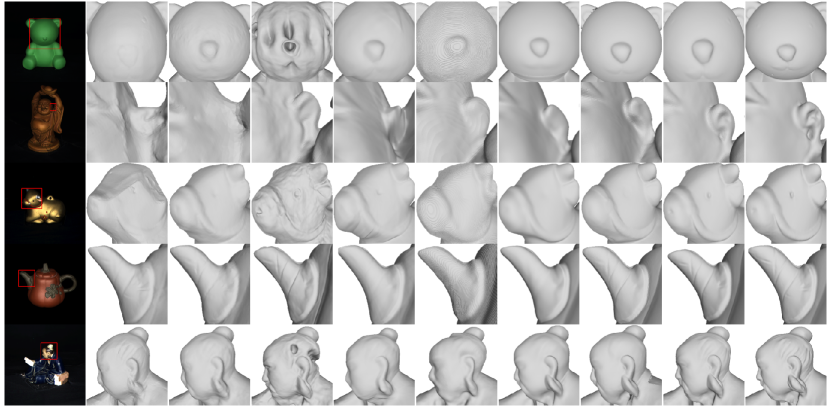
Figure 3: Qualitative comparison, on the DiLiGenT-MV dataset, between our results and the results obtained using state-of-the-art methods, with a zoom-in on parts of the meshes representing fine details. We use $20$ views per object for all methods. The methods highlighted in green are MVS-based, while the others are MVPS-based.

Table I shows the quantitative evaluation and comparison, in terms of CD and normal MAE, of these methods. In this experiment, we use $20$ views per object. Note, however, that MVPS methods use multiple images per view, each one captured under different lighting conditions. Our method uses only one image per view. The table clearly shows that our method significantly outperforms current state-of-the-art methods on all five objects by a large margin for both Chamfer distance and normal MAE metric. Our method improves the CD for $Buddha$ by $78\%$ to $4.82$mm. Moreover, our method improves the CD for the challenging $Reading$ object from $12.35$mm to $7.60$mm. A similar trend can be observed for the normal MAE where our method attains the lowest angular error for all five objects in the dataset.

	Input image	Ours		NeuS2 [44]		NeuS [40]

Figure 4: Qualitative comparison of surface reconstruction results on the BlendedMVS dataset.

IV-B2 Evaluation on BlendedMVS dataset

We undertake a qualitative and quantitative analysis of our method and compare its performance to state-of-the-art methods using BlendedMVS dataset [21], which is a multi-view stereo dataset of real objects. Since BlendedMVS is an MVS dataset, we only consider MVS methods such as NeuS [40] and its successor NeuS2 [44]. For the quantitative evaluation, we use the Chamfer distance and undertake two experiments. In the first one, we use all the views available for each object. In the second experiment, we only use $8$ views. Table II summarizes the results. Our method performs better than other methods in most cases using all views, while it outperforms all other methods when we only have sparse $8$ views. This shows that our method is particularly effective in sparse-view scenarios.

TABLE II: Quantitative evaluation, in terms of CD ($\downarrow$) of the reconstruction quality on the BlendedMVS dataset and comparison with the state-of-the-art MVS methods. Best results are highlighted as 1st and 2nd.

	Using all views			Using $8$ views
	Ours	NeuS	NeuS2	Ours	NeuS	NeuS2
Bear	2.27	3.13	3.25	3.56	3.91	4.34
Clock	2.54	2.77	2.92	5.78	7.09	7.41
Dog	2.48	2.76	3.06	4.64	5.16	6.02
Durian	2.18	3.17	3.34	6.67	7.12	7.66
Jade	3.47	4.27	4.06	6.29	8.50	8.05
Man	2.07	2.26	2.18	3.45	4.08	3.88
Stone	2.09	2.81	4.18	3.12	3.68	5.16
Fountain	3.21	3.65	4.44	5.54	7.61	5.49
Gundam	1.28	1.64	4.67	2.23	3.11	5.27
Mean	2.39	2.94	3.57	4.58	5.58	5.92

TABLE III: The quantitative comparison results of Chamfer Distances (CD$\downarrow$) on the DTU dataset for sparse views under large-overlap and little-overlap settings. Best results are highlighted as 1st, 2nd, and 3rd.

Scan ID	24	37	40	55	63	65	69	83	97	105	106	110	114	118	122	Mean
COLMAP [52]	2.88	3.47	1.74	2.16	2.63	3.27	2.78	3.63	3.24	3.49	2.46	1.24	1.59	2.72	1.87	2.61
SparseNeuS [49]	4.81	5.56	5.81	2.68	3.30	3.88	2.39	2.91	3.08	2.33	2.64	3.12	1.74	3.55	2.31	3.34
VolRecon [50]	3.05	4.45	3.36	3.09	2.78	3.68	3.01	2.87	3.07	2.55	3.07	2.77	1.59	3.44	2.51	3.02
NeuS [40]	4.11	5.40	5.10	3.47	2.68	2.01	4.52	8.59	5.09	9.42	2.20	4.84	0.49	2.04	4.20	4.28
VolSDF [39]	4.07	4.87	3.75	2.61	5.37	4.97	6.88	3.33	5.57	2.34	3.15	5.07	1.20	5.28	5.41	4.26
MonoSDF [47]	3.47	3.61	2.10	1.05	2.37	1.38	1.41	1.85	1.74	1.10	1.46	2.28	1.25	1.44	1.45	1.86
NeuSurf [51]	1.35	3.25	2.50	0.80	1.21	2.35	0.77	1.19	1.20	1.05	1.05	1.21	0.41	0.80	1.08	1.35
Gaussian Surfels [68]	4.96	4.72	4.41	3.84	4.84	4.38	5.56	6.49	4.75	5.39	4.42	6.76	4.25	3.31	4.16	4.82
Ours	1.54	2.01	1.46	0.74	2.14	1.25	0.75	0.92	1.13	0.88	0.78	0.95	0.56	0.70	0.82	1.11
(a) Sparse Multi-view Stereo with Little-overlap (PixelNeRF Setting)
Scan ID	24	37	40	55	63	65	69	83	97	105	106	110	114	118	122	Mean
COLMAP [52]	0.90	2.89	1.63	1.08	2.18	1.94	1.61	1.30	2.34	1.28	1.10	1.42	0.76	1.17	1.14	1.52
SparseNeuS [49]	2.17	3.29	2.74	1.67	2.69	2.42	1.58	1.86	1.94	1.35	1.50	1.45	0.98	1.86	1.87	1.96
VolRecon [50]	1.20	2.59	1.56	1.08	1.43	1.92	1.11	1.48	1.42	1.05	1.19	1.38	0.74	1.23	1.27	1.38
NeuS [40]	4.57	4.49	3.97	4.32	4.63	1.95	4.68	3.83	4.15	2.50	1.52	6.47	1.26	5.57	6.11	4.00
VolSDF [39]	4.03	4.21	6.12	0.91	8.24	1.73	2.74	1.82	5.14	3.09	2.08	4.81	0.60	3.51	2.18	3.41
MonoSDF [47]	2.85	3.91	2.26	1.22	3.37	1.95	1.95	5.53	5.77	1.10	5.99	2.28	0.65	2.65	2.44	2.93
NeuSurf [51]	0.78	2.35	1.55	0.75	1.04	1.68	0.60	1.14	0.98	0.70	0.74	0.49	0.39	0.75	0.86	0.99
Gaussian Surfels [68]	4.30	4.06	4.37	3.13	4.94	3.95	5.23	6.11	4.56	4.12	3.97	5.13	4.52	4.20	5.43	4.47
Ours	0.61	1.96	1.33	0.59	1.57	1.31	0.57	0.72	0.89	0.84	0.54	0.60	0.31	0.49	0.66	0.87
(b) Sparse Multi-view Stereo with Large-overlap (SparseNeuS Setting)

Fig. 4 shows a visual comparison of NeuS [40] and NeuS2 [44] with our method on three different objects from the BlendedMVS dataset, namely: Stone, Gundam, and Fountain. We observe that while NeuS2 [44] is significantly faster than the other two methods, it is unable to recover high-quality meshes of real-world objects. The reconstructed meshes have numerous errors and noise. In some instances, NeuS2 significantly fails when using specific views; see, for example, the second row of Fig. 4. While NeuS [40] outputs decent-quality meshes, we can see some artifacts at the top and shells of Stone (first row), and around the shoulders of Gundam (second row). Our method provides highly detailed and highly accurate meshes in regions such as the top of the ball in Stone, the separation between the arm and arm shield in Gundam, and the hand of the statue in Fountain.

IV-B3 Evaluation on the DTU dataset

We also evaluate the performance of our method on the DTU dataset, which is an MVS dataset. In this experiment, we are particularly interested in demonstrating the performance of our method in sparse MVS when there is a little overlap between the views and when there is a large overlap between the views. In both cases, we only use three views following PixelNeRF [67] and SparseNeuS [49] settings. Table III reports the comparison, in terms of CD, of our method against $8$ state-of-the-art methods including NeuSurf [51], which is based on neural surfaces, and Gaussian Surfels [68], which is based on Gaussian splatting. The former is specifically designed for sparse MVS settings. From this table, we can see that, on average, our method outperforms all the state-of-the-art methods both in the little as well as in the large overlap settings. We observe that in both settings, our method significantly outperforms Gaussian Surfels [68] in all scans and outperforms NeuSurf [51] in $12$ scans out of $15$.

Figures 3 and 4 in the Supplementary Material provide a visual comparison of the results of our method with the results of Gaussian Surfels [68]. As one can see, Gaussian Surfels significantly fail when in sparse multi-view stereo, both in the little-overlap setting (Figure 4) and in the large-overlap setting (Figure 5). Our method, on the other hand, recovers highly accurate 3D geometry in both settings.

IV-C Ablation study

In this section, we quantitatively and qualitatively analyze the importance of each component of the proposed method.

IV-C1 Normal supervision vs. depth supervision

In this paper, we estimate the surface normals for each input image by using the depth maps obtained using the of-the-shelf monocular depth estimator Depth Anything [1]. These normals are then used to supervise the 3D reconstruction of the surface geometry. Since we are using an off-the-shelf depth estimator from which normals are inferred, one can ask why we do not supervise our method directly with the estimated depth. What new information, which is not present in the depth maps, that the normal maps bring in? To demonstrate the importance of normal-based supervision, we undertake an ablation study in which we replace the normal loss with a depth loss. To do so, we first compute the surface points in world coordinates and then project them back to image coordinates to measure their depths. Finally, we supervise these points using the estimated sampled points from the Depth Anything depth estimation model.

BMVS Man Cow
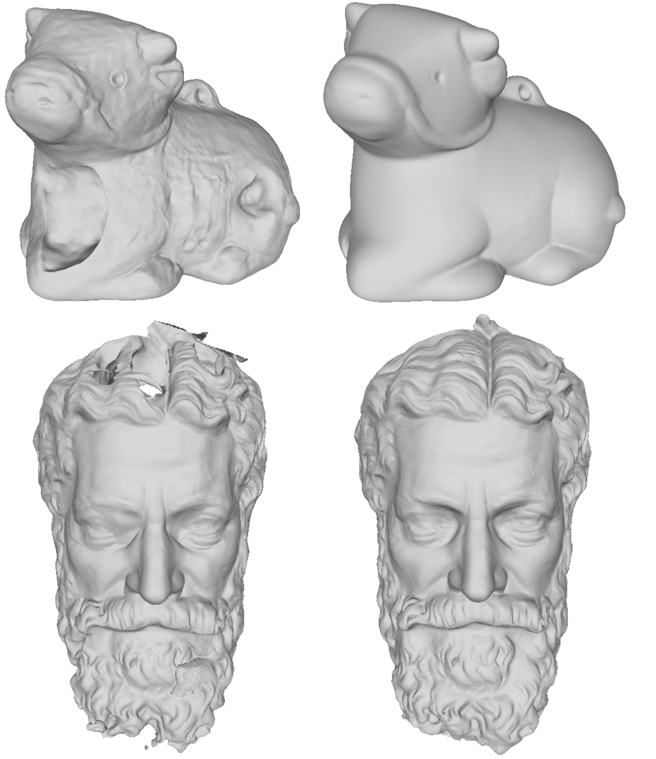
	Depth supervision	With normal supervision
		(Ours)

Figure 5: Comparison, on DiLiGenT-MV and BlendedMVS datasets, of the reconstruction quality when using depth supervision vs. normal (ours) supervision. When using depth supervision, we can clearly see artifacts in the form of holes or craters in the reconstructed meshes. However, when using the proposed normal-based supervision, we obtain high-quality reconstructions both in large areas (e.g., the cow body) as well as in areas that have fine details such as the eyes, hair, and beard of the BMVS man.

The last two rows of Table I show the accuracy of the reconstruction results, in terms of CD and normal MAE, when using normal supervision (second last row) vs. depth supervision (last row) on all the objects of the DiLiGenT-MV dataset. We can clearly see that supervision with normals outperforms depth-based supervision on both Chamfer distance and normal MAE by $51\%$ and $433\%$, respectively. This observation can also be visually confirmed in Figure 5, where we can clearly see that depth-based supervision produces holes or craters in the reconstructed mesh and distorts the geometry of their surfaces. We argue that this behavior is predictable since the 3D points used for 3D supervision do not carry information about the local geometry. On the other hand, first-order differential properties such as normals characterize the local geometry and thus ensure that the reconstructed surfaces are locally consistent and rich in geometric details.

IV-C2 Effect of the number of input views per object

(a) Bear	(b) Buddha	(c) Cow
(d) Pot2	(e) Reading

Figure 6: Quantitative comparison, on the DiLiGenT-MV dataset, of the performance of different methods when varying the number of input viewpoints from $20$ to $20$. Note that MVS methods such as ours and NeuS use one RGB image per view while MVPS methods use multiple images per view, each image is captured under different lighting conditions.

We evaluate how the performance of our method changes with the number of input views ($2,4,5,6,8,10,15$ and $20$ views) and compare it to existing methods such as RNb-NeuS [62], PS-NeRF [61], and NeuS [40].  Figure 6 shows how the Chamfer distance is affected by the number of views for each of the five objects from the DiLiGenT-MV dataset. Table IV provides the CD and normal MAE when using only two views. We can clearly see from Figure 6 and Table IV that while the performance of state-of-the-art methods degrades as the input views become sparser, our method shows stable performance even when using as few as two views, with only one RGB image per view. Moreover, the Chamfer distance of our method, when using only two views, significantly outperforms the current best multi-view photometric stereo model, namely RNb-NeuS [62].

TABLE IV: Results of different methods on the DiLiGenT-MV dataset when using only $2$ views with little overlap. Best results are highlighted as 1st, 2nd, and 3rd.

	Chamfer Dist$\downarrow$						Normal MAE$\downarrow$
Method	Bear	Buddha	Cow	Pot2	Reading	Average	Bear	Buddha	Cow	Pot2	Reading	Average
NeuS	142.44	71.55	130.19	131.58	156.26	126.40	35.84	37.23	32.25	32.37	42.85	36.11
PS-NeRF [61]	29.26	50.42	37.21	18.72	56.81	38.48	15.59	43.16	17.35	14.94	31.40	24.45
RNb-NeuS [62]	39.08	45.58	48.87	23.18	43.38	40.01	22.95	46.19	15.36	15.83	22.52	24.57
Ours	17.49	11.05	11.40	7.32	61.69	21.79	2.54	6.25	1.69	3.11	5.67	3.85
Ours (depth supervision)	116.62	165.57	132.31	90.66	111.13	123.26	58.18	76.08	65.60	35.35	69.04	60.85

Ours RNb-NeuS PS-NeRF NeuS
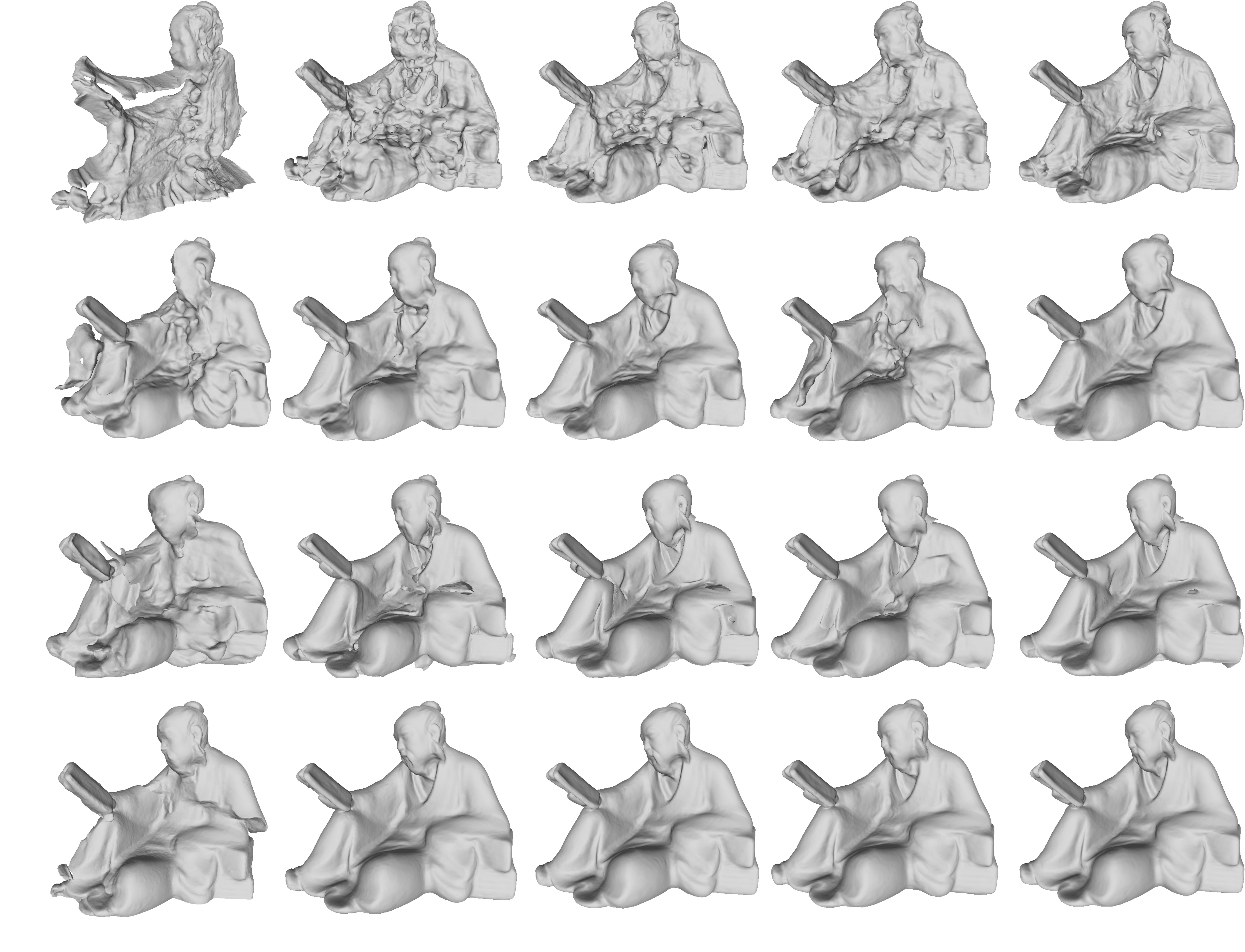
	2 views	5 views	10 views	15 views	20 views

Figure 7: Qualitative comparison of Reading between NeuS [40], PS-NeRF [61], RNb-NeuS [62] and our method for different numbers of input viewpoints.

Ours RNb-NeuS PS-NeRF NeuS
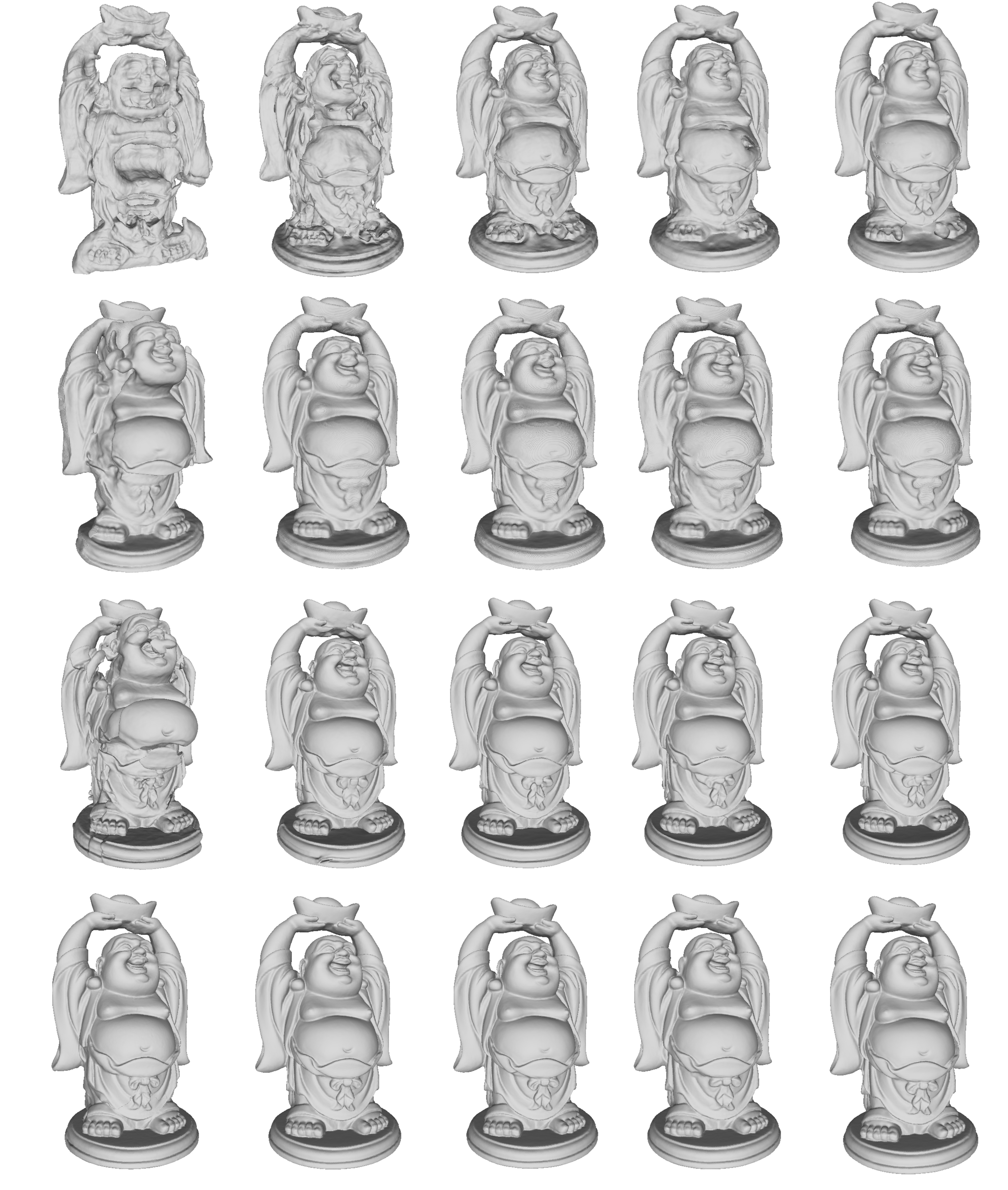
	2 views	5 views	10 views	15 views	20 views

Figure 8: Qualitative comparison of Buddha between NeuS [40], PS-NeRF [61], RNb-Neus [62] and our method, for different numbers of input viewpoints.

Since our method takes advantage of using surface normals as an additional supervision, it learns to better capture the local geometric details of the surface, such as the orientation and curvature at different points, even when the input views are sparse. This results in reconstructed surfaces that are smoother and more accurate, particularly in regions with high curvature or fine details. Figs. 7 and 8 visually show that while the reconstructed mesh quality deteriorates substantially for NeuS [40], PS-NeRF [61], and RNb-NeuS [62] as the input views become sparser (some of them such as NeuS just collapsed), our method outputs high-quality meshes even when the number of input views is as few as two.

V Conclusion

In this paper, we have proposed a new method for multi-view reconstruction of objects even in extremely sparse multi-view stereo scenarios where only as few as two images per object are available. We show that previous state-of-the-art multi-view stereo and multi-view photometric stereo methods produce 3D surfaces with missing parts and fail to recover fine details. We have demonstrated that incorporating high-order geometry cues in the form of surface normals results in highly accurate 3D surface reconstruction, even in situations where only as few as two RGB (front and back) images are available. Extensive evaluation on synthetic and real-world datasets shows that our method is able to recover high-fidelity meshes and outperforms, both qualitatively and quantitatively, the state-of-the-art multi-view stereo methods as well as multi-view photometric stereo.

Limitations. One main limitation of our method is that it only reconstructs parts that are visible from at least one camera. In other words, the proposed method does not infer invisible parts since it does not reason about the semantics of the shapes. Another limitation is computation time. Similar to NeuS [40] and most neural surfaces-based methods, our method takes a few hours to train over $300$ epochs. However, our method does not take advantage of CUDA acceleration as in [44]. Thus, as a future work, one will explore CUDA-based acceleration as well as multi-resolution hash encoding, which have the potential to improve the computation time from hours to seconds.

Appendix

This Supplementary Material provides additional results and evaluations that could not fit into the main manuscript. The dedicated anonymous Github site (https://sn-nir.github.io) provides the source code.

VI Effect of the number of views

Table V shows, in terms of Chamfer Distance (CD) and normal Mean Average Error (MAE), how our method is affected when reducing the number of views from $20$ to $4$. Compared to the state-of-the-art method on the DiLiGenT-MV dataset, we can clearly see that our method performs very well when we have a large number of views, outperforming even dense multiview photometric stereo methods (MVS). Importantly, unlike other methods, the performance of our method drops only slightly when we reducing the number of views from $20$ to $4$. Note that in this experiement, the views are distributed uniformly around the object. Thus, when they are sparse, they have little overlap. Yet, our method is able to recover the overall 3D shape as well as the surface details with very high accuracy.

TABLE V: Results of different methods on the DiLiGenT-MV dataset when using $15,10,8,6,5$ and $4$ views. Best results are highlighted as 1st, 2nd and 3rd.

	Chamfer Dist$\downarrow$						Normal MAE$\downarrow$
Method (with 15 views)	Bear	Buddha	Cow	Pot2	Reading	Average	Bear	Buddha	Cow	Pot2	Reading	Average
NeuS [40]	27.94	12.63	32.99	33.58	26.36	26.70	27.68	22.42	30.88	39.43	28.11	29.70
PS-NeRF [61]	7.49	10.82	15.37	8.03	20.69	12.48	6.77	19.02	10.97	12.00	13.89	12.53
RNb-NeuS [62]	36.32	8.78	39.39	5.93	14.32	20.95	3.45	13.66	4.57	6.96	9.31	7.59
Ours	9.19	7.79	10.15	6.35	8.34	8.36	1.11	4.10	1.20	2.02	4.11	2.51
Ours (depth supervision)	10.45	11.48	20.54	5.88	18.02	13.27	7.11	16.53	12.08	9.84	15.01	12.11

	Chamfer Dist$\downarrow$						Normal MAE$\downarrow$
Method (with 10 views)	Bear	Buddha	Cow	Pot2	Reading	Average	Bear	Buddha	Cow	Pot2	Reading	Average
NeuS [40]	38.62	15.48	55.45	47.58	25.13	27.94	22.12	27.88	33.18	38.34	28.16	27.94
PS-NeRF [61]	9.22	10.07	13.08	8.93	12.84	10.83	7.99	17.97	9.93	12.12	11.48	11.90
RNb-NeuS [62]	34.40	6.17	46.07	8.44	17.26	22.47	3.41	12.85	4.87	6.79	8.95	7.37
Ours	7.89	7.71	12.21	5.93	7.87	8.32	1.20	5.00	1.33	2.08	3.97	2.72
Ours (depth supervision)	13.32	12.72	22.90	20.13	23.53	18.52	15.07	23.01	22.89	17.69	22.37	20.21

	Chamfer Dist$\downarrow$						Normal MAE$\downarrow$
Method (with 8 views)	Bear	Buddha	Cow	Pot2	Reading	Average	Bear	Buddha	Cow	Pot2	Reading	Average
NeuS [40]	36.64	18.43	61.52	46.68	41.26	40.91	24.71	27.59	29.39	35.68	31.84	29.84
PS-NeRF [61]	8.61	10.68	15.51	8.53	15.76	11.82	8.08	18.16	11.14	12.60	12.65	12.52
RNb-NeuS [62]	38.31	7.79	46.91	12.58	17.85	24.68	3.49	12.95	5.05	7.79	8.55	7.56
Ours	9.09	8.06	12.52	4.56	7.35	8.31	1.08	4.22	1.27	2.09	4.67	2.66
Ours (depth supervision)	25.13	15.69	49.41	33.11	27.19	30.11	17.82	26.50	26.53	21.25	24.02	23.22

	Chamfer Dist$\downarrow$						Normal MAE$\downarrow$
Method (with 6 views)	Bear	Buddha	Cow	Pot2	Reading	Average	Bear	Buddha	Cow	Pot2	Reading	Average
NeuS [40]	42.86	20.12	63.24	49.26	40.46	43.18	21.69	30.78	27.36	32.01	31.40	28.65
PS-NeRF [61]	10.60	11.07	21.20	6.82	23.88	14.72	9.35	19.73	10.87	10.06	15.04	13.01
RNb-NeuS [62]	34.25	5.88	37.96	14.26	18.92	22.25	4.60	14.64	8.16	7.71	9.87	8.99
Ours	8.32	8.61	14.75	4.10	7.64	8.68	1.16	4.47	1.36	2.22	4.78	2.79
Ours (depth supervision)	30.28	17.56	37.22	29.60	26.58	28.25	18.33	35.28	27.68	20.69	25.21	24.44

	Chamfer Dist$\downarrow$						Normal MAE$\downarrow$
Method (5 views)	Bear	Buddha	Cow	Pot2	Reading	Average	Bear	Buddha	Cow	Pot2	Reading	Average
NeuS [40]	45.18	27.11	66.37	39.72	51.92	46.06	22.40	36.94	33.07	33.86	33.82	32.02
PS-NeRF [61]	11.97	12.43	21.78	9.42	16.37	14.39	9.21	19.17	12.89	13.41	13.97	13.73
RNb-NeuS [62]	29.00	7.65	41.26	9.34	23.54	22.16	78.10	15.23	6.20	8.29	10.92	23.75
Ours	8.89	8.72	11.52	4.56	7.58	7.11	1.27	4.73	1.44	2.16	4.18	2.76
Ours (depth supervision)	34.99	31.36	63.13	35.28	52.45	43.44	19.59	46.49	35.90	25.49	42.68	54.26

	Chamfer Dist$\downarrow$						Normal MAE$\downarrow$
Method (with 4 views)	Bear	Buddha	Cow	Pot2	Reading	Average	Bear	Buddha	Cow	Pot2	Reading	Average
NeuS [40]	60.76	40.10	66.14	39.52	49.18	51.14	30.79	39.46	30.76	32.97	33.92	33.58
PS-NeRF [61]	11.09	14.87	22.21	97.99	19.34	33.10	9.46	23.84	12.43	11.80	14.38	14.38
RNb-NeuS [62]	20.75	9.68	23.98	12.49	23.56	18.09	5.45	18.30	6.57	8.85	11.16	10.06
Ours	8.67	8.30	7.78	4.23	7.46	7.28	1.96	5.37	1.56	2.56	4.26	3.14
Ours (depth supervision)	57.98	39.68	70.01	39.83	38.54	49.21	26.74	55.07	43.90	31.15	39.15	39.20

VII Additional results

Figures 9 and 10 show two examples from the DiLiGenT-MV reconstructed from $20$ views. In this experiment, we also plot the vertex-wise reconstruction error, measured in terms of the deviation of the normals of the reconstructed mesh from those of the ground-truth mesh. As one can see, our method achieves significantly better reconstruction accuracy.

Ours	RNb-NeuS [62]	Kaya23 [66]	PS-NeRF [61]	Kaya22 [60]	NeuS [40]	Li19 [58]	Park16 [56]

Figure 9: Reconstructed 3D mesh and corresponding angular error of the Cow from the DiLiGenT-MV benchmark for 20 views.

Ours	RNb-NeuS [62]	Kaya23 [66]	PS-NeRF [61]	Kaya22 [60]	NeuS [40]	Li19 [58]	Park16 [56]

Figure 10: Reconstructed 3D mesh and corresponding angular error of the Pot2 from the DiLiGenT-MV benchmark for 20 views.

Figure 11: Qualitative comparison between our method and Gaussian Surfels [68] on the DTU dataset under little overlap setting.

Figure 12: Qualitative comparison between our method and Gaussian Surfels [68] on the DTU dataset under large overlap setting.

Finally, Figures 11 and 12 provide a visual comparison of the results of our method with the results of Gaussian Surfels [68]. As one can see Gaussian Surfels significantly fails when in sparse multiview stereo, both in the little-overlap setting (Figure 4) and in the large-overlap setting (Figure 5). Our method, on the other hand, recovers highly accurate 3D geometry in both settings.

References

- [1] L. Yang, B. Kang, Z. Huang, X. Xu, J. Feng, and H. Zhao, “Depth anything: Unleashing the power of large-scale unlabeled data,” in CVPR, 2024.
- [2] X.-F. Han, H. Laga, and M. Bennamoun, “Image-based 3d object reconstruction: State-of-the-art and trends in the deep learning era,” IEEE transactions on pattern analysis and machine intelligence, vol. 43, no. 5, pp. 1578–1604, 2021.
- [3] M. Kazhdan and H. Hoppe, “Screened poisson surface reconstruction,” ACM Trans. Graph., vol. 32, no. 3, jul 2013. [Online]. Available: https://doi.org/10.1145/2487228.2487237
- [4] P. Labatut, J.-P. Pons, and R. Keriven, “Efficient multi-view reconstruction of large-scale scenes using interest points, delaunay triangulation and graph cuts,” in 2007 IEEE 11th International Conference on Computer Vision, 2007, pp. 1–8.
- [5] W. E. Lorensen and H. E. Cline, “Marching Cubes: A High Resolution 3D Surface Construction Algorithm,” ACM SIGGRAPH Computer Graphics, Aug. 1987.
- [6] M. Attene and M. Spagnuolo, “Automatic surface reconstruction from point sets in space,” in Computer Graphics Forum, vol. 19, no. 3. Wiley Online Library, 2000, pp. 457–465.
- [7] R. Kolluri, J. R. Shewchuk, and J. F. O’Brien, “Spectral surface reconstruction from noisy point clouds,” in Proceedings of the 2004 Eurographics/ACM SIGGRAPH Symposium on Geometry Processing, ser. SGP ’04. New York, NY, USA: Association for Computing Machinery, 2004, p. 11–21. [Online]. Available: https://doi.org/10.1145/1057432.1057434
- [8] H. Huang, D. Li, H. Zhang, U. Ascher, and D. Cohen-Or, “Consolidation of unorganized point clouds for surface reconstruction,” ACM transactions on graphics (TOG), vol. 28, no. 5, pp. 1–7, 2009.
- [9] Y. Livny, F. Yan, M. Olson, B. Chen, H. Zhang, and J. El-Sana, “Automatic reconstruction of tree skeletal structures from point clouds,” in ACM SIGGRAPH Asia 2010 papers, 2010, pp. 1–8.
- [10] L. Nan and P. Wonka, “Polyfit: Polygonal surface reconstruction from point clouds,” in Proceedings of the IEEE International Conference on Computer Vision, 2017, pp. 2353–2361.
- [11] B. Curless and M. Levoy, “A volumetric method for building complex models from range images,” in Proceedings of the 23rd Annual Conference on Computer Graphics and Interactive Techniques, ser. SIGGRAPH ’96. New York, NY, USA: Association for Computing Machinery, 1996, p. 303–312. [Online]. Available: https://doi.org/10.1145/237170.237269
- [12] S. M. Seitz and C. R. Dyer, “Photorealistic scene reconstruction by voxel coloring,” International journal of computer vision, vol. 35, pp. 151–173, 1999.
- [13] L. Mescheder, M. Oechsle, M. Niemeyer, S. Nowozin, and A. Geiger, “Occupancy networks: Learning 3d reconstruction in function space,” in Proceedings of the IEEE/CVF conference on computer vision and pattern recognition, 2019, pp. 4460–4470.
- [14] J. J. Park, P. Florence, J. Straub, R. Newcombe, and S. Lovegrove, “Deepsdf: Learning continuous signed distance functions for shape representation,” in Proceedings of the IEEE/CVF conference on computer vision and pattern recognition, 2019, pp. 165–174.
- [15] J. Chibane, G. Pons-Moll et al., “Neural unsigned distance fields for implicit function learning,” Advances in Neural Information Processing Systems, vol. 33, pp. 21 638–21 652, 2020.
- [16] M. Niemeyer, L. Mescheder, M. Oechsle, and A. Geiger, “Differentiable volumetric rendering: Learning implicit 3d representations without 3d supervision,” in Proceedings of the IEEE/CVF conference on computer vision and pattern recognition, 2020, pp. 3504–3515.
- [17] L. Yariv, Y. Kasten, D. Moran, M. Galun, M. Atzmon, B. Ronen, and Y. Lipman, “Multiview neural surface reconstruction by disentangling geometry and appearance,” Advances in Neural Information Processing Systems, vol. 33, pp. 2492–2502, 2020.
- [18] S. Peng, M. Niemeyer, L. Mescheder, M. Pollefeys, and A. Geiger, “Convolutional occupancy networks,” in Computer Vision–ECCV 2020: 16th European Conference, Glasgow, UK, August 23–28, 2020, Proceedings, Part III 16. Springer, 2020, pp. 523–540.
- [19] Q. Wang, Z. Wang, K. Genova, P. P. Srinivasan, H. Zhou, J. T. Barron, R. Martin-Brualla, N. Snavely, and T. Funkhouser, “Ibrnet: Learning multi-view image-based rendering,” in Proceedings of the IEEE/CVF Conference on Computer Vision and Pattern Recognition, 2021, pp. 4690–4699.
- [20] M. Li, Z. Zhou, Z. Wu, B. Shi, C. Diao, and P. Tan, “Multi-view photometric stereo: A robust solution and benchmark dataset for spatially varying isotropic materials,” Trans. Img. Proc., vol. 29, p. 4159–4173, jan 2020. [Online]. Available: https://doi.org/10.1109/TIP.2020.2968818
- [21] Y. Yao, Z. Luo, S. Li, J. Zhang, Y. Ren, L. Zhou, T. Fang, and L. Quan, “Blendedmvs: A large-scale dataset for generalized multi-view stereo networks,” Computer Vision and Pattern Recognition (CVPR), 2020.
- [22] R. Jensen, A. Dahl, G. Vogiatzis, E. Tola, and H. Aanæs, “Large scale multi-view stereopsis evaluation,” in Proceedings of the IEEE conference on computer vision and pattern recognition, 2014, pp. 406–413.
- [23] H. Laga, L. V. Jospin, F. Boussaid, and M. Bennamoun, “A survey on deep learning techniques for stereo-based depth estimation,” IEEE transactions on pattern analysis and machine intelligence, vol. 44, no. 4, pp. 1738–1764, 2022.
- [24] Y. Furukawa and J. Ponce, “Accurate, dense, and robust multiview stereopsis,” IEEE Transactions on Pattern Analysis and Machine Intelligence, vol. 32, no. 8, pp. 1362–1376, 2010.
- [25] M. Goesele, N. Snavely, B. Curless, H. Hoppe, and S. M. Seitz, “Multi-view stereo for community photo collections,” in 2007 IEEE 11th International Conference on Computer Vision, 2007, pp. 1–8.
- [26] A. Kar, C. Häne, and J. Malik, “Learning a multi-view stereo machine,” Advances in neural information processing systems, vol. 30, 2017.
- [27] M. Ji, J. Gall, H. Zheng, Y. Liu, and L. Fang, “Surfacenet: An end-to-end 3d neural network for multiview stereopsis,” in 2017 IEEE International Conference on Computer Vision (ICCV), 2017, pp. 2326–2334.
- [28] Y. Yao, Z. Luo, S. Li, T. Fang, and L. Quan, “Mvsnet: Depth inference for unstructured multi-view stereo,” 2018.
- [29] X. Gu, Z. Fan, S. Zhu, Z. Dai, F. Tan, and P. Tan, “Cascade cost volume for high-resolution multi-view stereo and stereo matching,” in Proceedings of the IEEE/CVF conference on computer vision and pattern recognition, 2020, pp. 2495–2504.
- [30] Y. Zhang, J. Zhu, and L. Lin, “Multi-view stereo representation revist: Region-aware mvsnet,” in Proceedings of the IEEE/CVF Conference on Computer Vision and Pattern Recognition, 2023, pp. 17 376–17 385.
- [31] Y. Wang, Z. Zeng, T. Guan, W. Yang, Z. Chen, W. Liu, L. Xu, and Y. Luo, “Adaptive patch deformation for textureless-resilient multi-view stereo,” in Proceedings of the IEEE/CVF Conference on Computer Vision and Pattern Recognition, 2023, pp. 1621–1630.
- [32] Y. Ding, W. Yuan, Q. Zhu, H. Zhang, X. Liu, Y. Wang, and X. Liu, “Transmvsnet: Global context-aware multi-view stereo network with transformers,” in Proceedings of the IEEE/CVF Conference on Computer Vision and Pattern Recognition, 2022, pp. 8585–8594.
- [33] R. Peng, R. Wang, Z. Wang, Y. Lai, and R. Wang, “Rethinking depth estimation for multi-view stereo: A unified representation,” in Proceedings of the IEEE/CVF Conference on Computer Vision and Pattern Recognition, 2022, pp. 8645–8654.
- [34] S. Cheng, Z. Xu, S. Zhu, Z. Li, L. E. Li, R. Ramamoorthi, and H. Su, “Deep stereo using adaptive thin volume representation with uncertainty awareness,” in Proceedings of the IEEE/CVF Conference on Computer Vision and Pattern Recognition, 2020, pp. 2524–2534.
- [35] J. Yang, W. Mao, J. M. Alvarez, and M. Liu, “Cost volume pyramid based depth inference for multi-view stereo,” in Proceedings of the IEEE/CVF conference on computer vision and pattern recognition, 2020, pp. 4877–4886.
- [36] Z. Zhang, R. Peng, Y. Hu, and R. Wang, “Geomvsnet: Learning multi-view stereo with geometry perception,” in Proceedings of the IEEE/CVF Conference on Computer Vision and Pattern Recognition, 2023, pp. 21 508–21 518.
- [37] B. Mildenhall, P. P. Srinivasan, M. Tancik, J. T. Barron, R. Ramamoorthi, and R. Ng, “Nerf: Representing scenes as neural radiance fields for view synthesis,” Communications of the ACM, vol. 65, no. 1, pp. 99–106, 2021.
- [38] M. Oechsle, S. Peng, and A. Geiger, “Unisurf: Unifying neural implicit surfaces and radiance fields for multi-view reconstruction,” in Proceedings of the IEEE/CVF International Conference on Computer Vision, 2021, pp. 5589–5599.
- [39] L. Yariv, J. Gu, Y. Kasten, and Y. Lipman, “Volume rendering of neural implicit surfaces,” Advances in Neural Information Processing Systems, vol. 34, pp. 4805–4815, 2021.
- [40] P. Wang, L. Liu, Y. Liu, C. Theobalt, T. Komura, and W. Wang, “NeuS: Learning Neural Implicit Surfaces by Volume Rendering for Multi-view Reconstruction,” arXiv preprint arXiv:2106.10689, 2021.
- [41] A. Pumarola, E. Corona, G. Pons-Moll, and F. Moreno-Noguer, “D-nerf: Neural radiance fields for dynamic scenes,” in Proceedings of the IEEE/CVF Conference on Computer Vision and Pattern Recognition, 2021, pp. 10 318–10 327.
- [42] J. Gu, M. Jiang, H. Li, X. Lu, G. Zhu, S. A. A. Shah, L. Zhang, and M. Bennamoun, “Ue4-nerf: Neural radiance field for real-time rendering of large-scale scene,” Advances in Neural Information Processing Systems, vol. 36, 2024.
- [43] T. Müller, A. Evans, C. Schied, and A. Keller, “Instant neural graphics primitives with a multiresolution hash encoding,” ACM Trans. Graph., vol. 41, no. 4, pp. 102:1–102:15, Jul. 2022. [Online]. Available: https://doi.org/10.1145/3528223.3530127
- [44] Y. Wang, Q. Han, M. Habermann, K. Daniilidis, C. Theobalt, and L. Liu, “Neus2: Fast learning of neural implicit surfaces for multi-view reconstruction,” in Proceedings of the IEEE/CVF International Conference on Computer Vision, 2023, pp. 3295–3306.
- [45] F. Darmon, B. Bascle, J.-C. Devaux, P. Monasse, and M. Aubry, “Improving neural implicit surfaces geometry with patch warping,” in Proceedings of the IEEE/CVF Conference on Computer Vision and Pattern Recognition, 2022, pp. 6260–6269.
- [46] Z. Li, T. Müller, A. Evans, R. H. Taylor, M. Unberath, M.-Y. Liu, and C.-H. Lin, “Neuralangelo: High-fidelity neural surface reconstruction,” in Proceedings of the IEEE/CVF Conference on Computer Vision and Pattern Recognition, 2023, pp. 8456–8465.
- [47] Z. Yu, S. Peng, M. Niemeyer, T. Sattler, and A. Geiger, “Monosdf: Exploring monocular geometric cues for neural implicit surface reconstruction,” Advances in Neural Information Processing Systems (NeurIPS), 2022.
- [48] Q. Fu, Q. Xu, Y. S. Ong, and W. Tao, “Geo-neus: Geometry-consistent neural implicit surfaces learning for multi-view reconstruction,” Advances in Neural Information Processing Systems, vol. 35, pp. 3403–3416, 2022.
- [49] X. Long, C. Lin, P. Wang, T. Komura, and W. Wang, “SparseNeuS: Fast generalizable neural surface reconstruction from sparse views,” in European Conference on Computer Vision. Springer, 2022, pp. 210–227.
- [50] Y. Ren, T. Zhang, M. Pollefeys, S. Süsstrunk, and F. Wang, “Volrecon: Volume rendering of signed ray distance functions for generalizable multi-view reconstruction,” in Proceedings of the IEEE/CVF Conference on Computer Vision and Pattern Recognition, 2023, pp. 16 685–16 695.
- [51] H. Huang, Y. Wu, J. Zhou, G. Gao, M. Gu, and Y.-S. Liu, “NeuSurf: On-Surface Priors for Neural Surface Reconstruction from Sparse Input Views,” in Proceedings of the AAAI Conference on Artificial Intelligence, vol. 38, no. 3, 2024, pp. 2312–2320.
- [52] J. L. Schonberger and J.-M. Frahm, “Structure-from-motion revisited,” in Proceedings of the IEEE conference on computer vision and pattern recognition, 2016, pp. 4104–4113.
- [53] J. Lim, J. Ho, M.-H. Yang, and D. Kriegman, “Passive photometric stereo from motion,” in Tenth IEEE International Conference on Computer Vision (ICCV’05) Volume 1, vol. 2. IEEE, 2005, pp. 1635–1642.
- [54] C. Hernandez, G. Vogiatzis, and R. Cipolla, “Multiview photometric stereo,” IEEE Transactions on Pattern Analysis and Machine Intelligence, vol. 30, no. 3, pp. 548–554, 2008.
- [55] C. Wu, Y. Liu, Q. Dai, and B. Wilburn, “Fusing multiview and photometric stereo for 3d reconstruction under uncalibrated illumination,” IEEE transactions on visualization and computer graphics, vol. 17, no. 8, pp. 1082–1095, 2010.
- [56] J. Park, S. N. Sinha, Y. Matsushita, Y.-W. Tai, and I. S. Kweon, “Robust multiview photometric stereo using planar mesh parameterization,” IEEE transactions on pattern analysis and machine intelligence, vol. 39, no. 8, pp. 1591–1604, 2016.
- [57] F. Logothetis, R. Mecca, and R. Cipolla, “A differential volumetric approach to multi-view photometric stereo,” in Proceedings of the IEEE/CVF International Conference on Computer Vision, 2019, pp. 1052–1061.
- [58] M. Li, Z. Zhou, Z. Wu, B. Shi, C. Diao, and P. Tan, “Multi-view photometric stereo: A robust solution and benchmark dataset for spatially varying isotropic materials,” Trans. Img. Proc., vol. 29, p. 4159–4173, jan 2020. [Online]. Available: https://doi.org/10.1109/TIP.2020.2968818
- [59] B. Kaya, S. Kumar, F. Sarno, V. Ferrari, and L. Van Gool, “Neural radiance fields approach to deep multi-view photometric stereo,” in Proceedings of the IEEE/CVF winter conference on applications of computer vision, 2022, pp. 1965–1977.
- [60] B. Kaya, S. Kumar, C. Oliveira, V. Ferrari, and L. Van Gool, “Uncertainty-aware deep multi-view photometric stereo,” in Proceedings of the IEEE/CVF Conference on Computer Vision and Pattern Recognition, 2022, pp. 12 601–12 611.
- [61] W. Yang, G. Chen, C. Chen, Z. Chen, and K.-Y. K. Wong, “PS-NeRF: Neural inverse rendering for multi-view photometric stereo,” in European Conference on Computer Vision. Springer, 2022, pp. 266–284.
- [62] B. Brument, R. Bruneau, Y. Quéau, J. Mélou, F. Lauze, J.-D. Durou, and L. Calvet, “Rnb-neus: Reflectance and normal based reconstruction with neus,” in Proceedings of the IEEE/CVF International Conference on Computer Vision, 2024.
- [63] N. Max, “Optical models for direct volume rendering,” IEEE Transactions on Visualization and Computer Graphics, vol. 1, no. 2, pp. 99–108, 1995.
- [64] M. Tancik, P. Srinivasan, B. Mildenhall, S. Fridovich-Keil, N. Raghavan, U. Singhal, R. Ramamoorthi, J. Barron, and R. Ng, “Fourier features let networks learn high frequency functions in low dimensional domains,” Advances in neural information processing systems, vol. 33, pp. 7537–7547, 2020.
- [65] A. Gropp, L. Yariv, N. Haim, M. Atzmon, and Y. Lipman, “Implicit geometric regularization for learning shapes,” arXiv preprint arXiv:2002.10099, 2020.
- [66] B. Kaya, S. Kumar, C. Oliveira, V. Ferrari, and L. V. Gool, “Multi-view photometric stereo revisited,” in 2023 IEEE/CVF Winter Conference on Applications of Computer Vision (WACV). Los Alamitos, CA, USA: IEEE Computer Society, jan 2023, pp. 3125–3134. [Online]. Available: https://doi.ieeecomputersociety.org/10.1109/WACV56688.2023.00314
- [67] A. Yu, V. Ye, M. Tancik, and A. Kanazawa, “pixelnerf: Neural radiance fields from one or few images,” in Proceedings of the IEEE/CVF Conference on Computer Vision and Pattern Recognition, 2021, pp. 4578–4587.
- [68] P. Dai, J. Xu, W. Xie, X. Liu, H. Wang, and W. Xu, “High-quality surface reconstruction using gaussian surfels,” in SIGGRAPH 2024 Conference Papers. Association for Computing Machinery, 2024.