Auto-Multilift: Distributed Learning and Control for Cooperative Load Transportation With Quadrotors

Abstract

Designing motion control and planning algorithms for multilift systems remains challenging due to the complexities of dynamics, collision avoidance, actuator limits, and scalability. Existing methods that use optimization and distributed techniques effectively address these constraints and scalability issues. However, they often require substantial manual tuning, leading to suboptimal performance. This paper proposes Auto-Multilift, a novel framework that automates the tuning of model predictive controllers (MPCs) for multilift systems. We model the MPC cost functions with deep neural networks (DNNs), enabling fast online adaptation to various scenarios. We develop a distributed policy gradient algorithm to train these DNNs efficiently in a closed-loop manner. Central to our algorithm is distributed sensitivity propagation, which parallelizes gradient computation across quadrotors, focusing on actual system state sensitivities relative to key MPC parameters. We also provide theoretical guarantees for the convergence of this algorithm. Extensive simulations show rapid convergence and favorable scalability to a large number of quadrotors. Our method outperforms a state-of-the-art open-loop MPC tuning approach by effectively learning adaptive MPCs from trajectory tracking errors and handling the unique dynamics couplings within the multilift system. Additionally, our framework can learn an adaptive reference for reconfigurating the system when traversing through multiple narrow slots.

Supplementary Material

The source code of this work is available at https://github.com/RCL-NUS/Auto-Multilift.

I Introduction

Aerial transportation with multiple quadrotors typically offers greater load capacity and enhanced system robustness than employing a single quadrotor. Cables represent a promising mechanism for attaching the load to the quadrotors because they are lightweight, easy to design, and particularly suited for large-scale load deployment [1]. The multilift system, in which a group of quadrotors cooperatively transports a cable-suspended load (see Fig. 1-a), has therefore received increasing attention for potential applications such as rescue operations and logistics [2, 3, 4, 5].

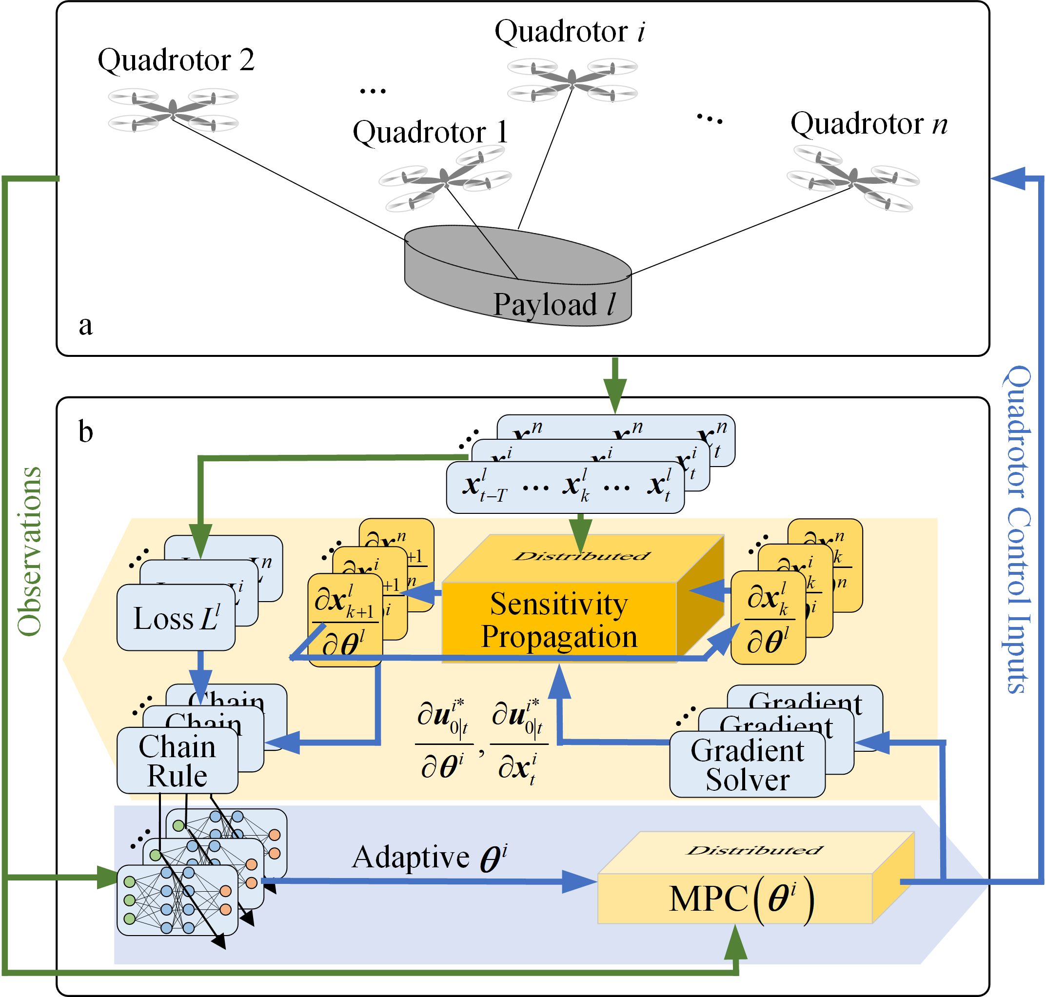
Figure 1: Illustration of a multilift system and Auto-Multilift learning pipelines. (a) Components and structure of a typical multilift system; (b) A block diagram of the proposed framework. We fuse DNNs with distributed MPC controllers to obtain adaptive cost function parameters online. These DNNs can be trained efficiently in a distributed and close-loop manner. This is achieved through distributed sensitivity propagation, a key module in our method that computes actual state sensitivities in parallel across the quadrotors.

Despite its advantages, the multilift system faces unique challenges due to the cables. The quadrotors’ motions are constrained by the cable length when taut and dynamically coupled with the load through the cable tensions. Moreover, the cables impart a hybrid nature to the system during transitions between slack and taut conditions, which significantly complicates the dynamics. These dynamic couplings and constraints require careful coordination among the quadrotors to maintain safe inter-robot separation and minimize slack-taut transitions. Other challenges include managing the quadrotor’s control constraints, avoiding obstacles, and scaling to a large number of quadrotors.

Research on motion planning and control of the multilift system has progressed over the years. Early works assumed the load as a point mass and treated the tensions as external disturbances on the quadrotors [6, 7]. Disturbance observers were used to estimate and counteract the tensions for maintaining the quadrotors’ trajectory tracking performance. This control method, which does not require a load model for simplicity, has recently regained attention [8, 9, 10]. However, ignoring the load dynamics in control design can compromise the system’s maneuverability, restricting this method to quasi-static or slow flights. To improve control performance in agile flights, Lee et al. [11, 12] developed a geometric control method that explicitly incorporates the dynamic couplings between the quadrotors and a point-mass load. Additionally, Jackson et al. [13] tackled the collision-free motion planning problem for a point mass load and proposed a distributed optimization approach that parallelizes trajectory planning across quadrotors. Nevertheless, methods based on the point mass assumption are limited to special cases where the load’s shape is negligible compared to the cable length, a condition often overly conservative for practical use.

On the other hand, treating the load as a rigid body with 6 degree-of-freedom (DoF) is more realistic but complicates the design of motion planning and control strategies. Achieving arbitrary control of a rigid-body load in 6 DoF requires at least three quadrotors [14]. A multilift system with more than two quadrotors introduces redundancy in the cable tensions [15], leading to their non-unique distribution across the quadrotors. In [16, 17, 18], the authors proposed the minimum-norm solution for distributing the cable tensions. In contrast, Geng et al. [19, 20] exploited this redundancy for a multilift system with four quadrotors to achieve optimal tension distribution while maintaining safe inter-rotor separation and respecting the quadrotor’s thrust limits. Furthermore, recent works [21, 22] included this redundancy in a centralized MPC framework, which not only ensures these safety constraints but also improves the system’s maneuverability by fully accounting for the nonlinear system dynamics. In addition, Geng et al. [23] recently developed an optimal motion planning method, aiming for even tension distribution and system dynamics compliance. However, its assumption of small load attitude angles prevents applicability to large load attitude maneuvers.

As demonstrated in the above works [13, 19, 20, 21, 22, 23], optimization methods are effective for multilift systems due to their ability to manage constraints and nonlinear dynamics. However, their performance significantly depends on the tuning of hyperparameters, including the weightings and references in cost functions. This tuning typically requires extensive manual effort, complicated by the large number of parameters and their dynamic interconnections from the cables. To simplify this, it often involves conservative assumptions such as treating the load as a point mass, assuming quasi-static flight, and even tension distribution, which can lead to suboptimal results. The challenge of manually selecting these parameters increases with more quadrotors and when their optimal values are dynamic and interconnected, such as when the load’s mass distribution is non-uniform and the system must dynamically adjust its configuration to avoid obstacles.

In this paper, we propose Auto-Multilift, a novel framework designed to automate the tuning of MPCs for multilift systems. We employ DNNs to dynamically adjust the weightings and references online within the MPC cost functions and present a highly efficient approach for training these DNNs using advanced machine learning techniques. Our method integrates the benefits of model-based control with end-to-end learning. Fig. 1-b illustrates the block diagram of Auto-Multilift and its learning pipelines. In the forward pass, distributed MPCs with these adaptive hyperparameters solve open-loop optimal control problems in parallel to generate control trajectories for a future horizon, but only the first control commands are applied to the system. In the backward pass, we develop a distributed policy gradient algorithm to efficiently train these DNNs. Central to our algorithm is distributed sensitivity propagation (DSP), which calculates the system state sensitivities relative to these hyperparameters using the closed-loop states and the gradients of the first control commands. We employ and tailor Safe-PDP [24] to obtain the gradients. These sensitivities, capturing the unique dynamics couplings within the multilift system, are solved in parallel, enabling the efficient training of the DNNs in a distributed and closed-loop manner. They also allow for the formulation of a loss function that evaluates performance over a time interval longer than the MPC’s horizon. More importantly, the proposed DSP algorithm can converge in finite iterations with theoretical guarantees.

Interest in learning for MPC has burgeoned, with advances like differentiable MPC [25], PDP [26], Safe-PDP [24]. Compared to differentiable MPC, PDP offers greater computational efficiency by recursively computing the MPC gradient via implicit differentiation of Pontryagin’s maximum principle. This technique, extended to constrained optimal control problems by Safe-PDP, has also been applied to learning cooperative control policies for multi-agent systems without dynamic couplings among agents [27, 28]. However, all these methods use open-loop state trajectories obtained by solving the MPC problem once per training episode, typically confining them to imitation learning that heavily relies on expert demonstrations. Conversely, using closed-loop state trajectories allows for broader training settings, such as reinforcement learning. Various closed-loop MPC learning strategies have been developed, including sampling-based methods [29, 30], black-box optimization methods [31, 32, 33], and Actor-Critic MPC [34]. Recently, Tao et al. [35] sought to enhance training efficiency by integrating differentiable MPC [25] with Diff-Tune [36], which computes the closed-loop state gradient relative to the MPC hyperparameters via sensitivity propagation. Our work contributes to this collection by providing a distributed, closed-loop MPC learning framework for multi-agent systems with strong dynamic couplings and constraints among agents.

We evaluate the effectiveness of Auto-Multilift through extensive simulations that account for realistic effects such as cable elasticity and motor dynamics. The proposed DSP algorithm converges in just a few steps, with convergence speed unaffected by the number of quadrotors, ensuring scalability to large multilift systems. In a complex simulation with up to six quadrotors transporting a load with non-uniform mass distribution, we demonstrate that our framework effectively learns adaptive MPC weightings from trajectory tracking errors. These weightings optimally distribute the cable tensions among the quadrotors to maintain the load attitude. This simulation also underscores the importance of using DSP in learning MPCs for multilift systems. Compared to training with Safe-PDP [24] alone, our method offers more stable performance and reduces the tracking errors by up to $70\%$. Finally, we perform a challenging obstacle avoidance simulation, showing that Auto-Multilift can learn an adaptive tension reference for MPCs. This capability enables the system to reconfigure itself while passing through multiple narrow slots with heights shorter than the cable length.

In summary, our main contributions are as follows:

1. We propose Auto-Multilift, a distributed and closed-loop learning framework that automatically tunes various MPC hyperparameters, modeled by DNNs, for multilift systems and adapts to different flight scenarios.

2. We develop a distributed sensitivity propagation (DSP) algorithm that efficiently computes the close-loop state sensitivities relative to the MPC hyperparameters in parallel. The convergence of this algorithm is theoretically justified.

3. We design a distributed policy gradient algorithm to train these DNNs directly from the system tracking errors in a distributed and closed-loop manner. It consists of DSP and MPC gradient solvers, the latter derived by tailoring Safe-PDP [24].

4. We conduct extensive simulations to showcase the fast convergence, the scalability, the effective closed-loop learning, and the improved learning stability and trajectory tracking performance over the state-of-the-art open-loop MPC tuning method.

The rest of this paper is organized as follows. Section II establishes the multilift system model and designs the MPC controllers. Section III formulates the Auto-Multilift problem. In Section IV, we detail the development of the DSP algorithm. Section V designs the distributed policy gradient algorithm. Simulation results are reported in Section VI. We discuss the advantages and disadvantages of our method in Section VII and conclude this paper in Section VIII.

II Preliminaries

II-A Multilift Model

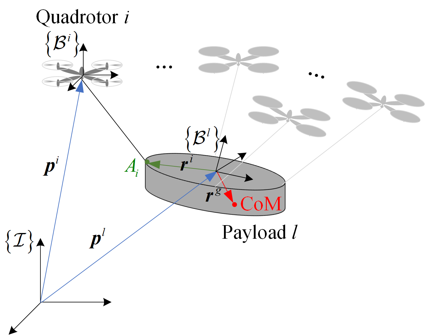
Figure 2: Illustration of the multilift system. Let $\mathcal{I}$, $\mathcal{B}^{l}$, and $\mathcal{B}^{i}$ denote the world frame, the body frame attached to the load, and the body frame attached to the $i$-th quadrotor, respectively.

We consider a multilift system with $n$ quadrotors and a rigid-body load. Each quadrotor is connected to an attachment point on the load via an elastic cable. For example, as shown in Fig. 2, the $i$-th quadrotor is linked to the attachment point $A_{i},\forall i\in{\cal I}_{q}$ with ${\cal I}_{q}=\left\{1,\cdots,n\right\}$ denoting the indices of the quadrotors. Each quadrotor is modeled as a 6 DoF rigid-body with the mass $m^{i}\in\mathbb{R}_{+}$ and the moment of inertia $\mathbf{J}^{i}\in\mathbb{R}^{3\times 3}$. We assume that each cable is attached to the center-of-mass (CoM) of the quadrotor, producing only a tension force acting on it. For the $i$-th quadrotor, $\forall i\in{\cal I}_{q}$, let $\bm{p}^{i}\in\mathbb{R}^{3}$ denote the CoM in $\mathcal{I}$, $\bm{v}^{i}\in\mathbb{R}^{3}$ the velocity of the CoM in $\mathcal{I}$, $\bm{q}^{i}\in\mathbb{R}^{4}$ the quaternion, and ${\bm{\omega}}^{i}\in\mathbb{R}^{3}$ the angular velocity in $\mathcal{B}^{i}$. The quadrotor’s dynamics model is given by

$$\dot{\bm{p}}^{i} ={\bm{v}}^{i},$$ (1a)

$$\dot{\bm{v}}^{i} =\frac{1}{m^{i}}\left(-{m^{i}g{\bm{e}}_{3}+{\mathbf{R}_{i}}f^{i}{\bm{e}}_{3}+{{\bm{T}}^{i,l}}}\right),$$ (1b)

$$\dot{\bm{q}}^{i} =\frac{1}{2}{\bm{\Omega}}\left({\bm{\omega}}^{i}\right){\bm{q}}^{i},$$ (1c)

$$\dot{\bm{\omega}}^{i} ={{\left({\mathbf{J}}^{i}\right)}^{-1}}\left({-{\left(\bm{\omega}^{i}\right)^{\times}}{\mathbf{J}}^{i}\left(\bm{\omega}^{i}\right)+\bm{\tau}^{i}}\right)$$ (1d)

where $g$ is the gravitational acceleration, ${\bm{e}}_{3}={\left[{0,0,1}\right]}^{T}$, $\mathbf{R}_{i}:={\mathbf{R}\left(\bm{q}^{i}\right)}\in SO\left(3\right)$ is the rotation matrix with $\bm{q}^{i}$ from $\mathcal{B}^{i}$ to $\mathcal{I}$, ${\bm{T}}^{i,l}\in\mathbb{R}^{3}$ is the $i$-th cable tension in $\mathcal{I}$, $\left(\bm{\omega}^{i}\right)^{\times}$ denotes the skew-symmetric matrix form of $\bm{\omega}^{i}$ as an element of the Lie algebra $\mathfrak{so}(3)$, $f^{i}\in\mathbb{R}_{+}$ and $\bm{\tau}^{i}\in\mathbb{R}^{3}$ are the total thrust and control torque produced by the quadrotor’s four motors in $\mathcal{B}^{i}$, respectively, and ${\bm{\Omega}}\left({\bm{\omega}}^{i}\right)$ is given by

$$\bm{\Omega}\left({\bm{\omega}}^{i}\right)=\begin{bmatrix}0&-\left({\bm{\omega}}^{i}\right)^{T}\\ {\bm{\omega}}^{i}&-\left({\bm{\omega}}^{i}\right)^{\times}\end{bmatrix}.$$

We model the load as a 6 DoF rigid-body with the mass $m^{l}\in\mathbb{R}_{+}$ and the moment of inertia $\mathbf{J}^{l}\in\mathbb{R}^{3\times 3}$. The load’s body frame $\mathcal{B}^{l}$ is built at its geometric center (GC), which can be easily determined when using a regular shaped container for load transportation, commonly seen in scenarios such as logistics. In pursuit of more realistic modelling, we discard the conservative assumption of uniform mass distribution of the load, resulting in a bias vector ${\bm{r}}^{g}\in\mathbb{R}^{3}$ for the load’s CoM in $\mathcal{B}^{l}$. Let $\bm{p}^{l}\in\mathbb{R}^{3}$ denote the position of the GC in $\mathcal{I}$, $\bm{v}^{l}\in\mathbb{R}^{3}$ the velocity of the GC in $\mathcal{B}^{l}$, $\bm{q}^{l}\in\mathbb{R}^{4}$ the quaternion of the load’s attitude, $\bm{\omega}^{l}\in\mathbb{R}^{3}$ the angular velocity of the load in $\mathcal{B}^{l}$. The load’s dynamics model is given by

$$\dot{\bm{p}}^{l} =\mathbf{R}_{l}{\bm{v}}^{l},$$ (2a)

$$\begin{split}\dot{\bm{v}}^{l}&=-\left(\dot{\bm{\omega}}^{l}\right)^{\times}{\bm{r}}^{g}-\left(\bm{\omega}^{l}\right)^{\times}{\bm{v}}^{l}-\left(\bm{\omega}^{l}\right)^{\times}\left(\left(\bm{\omega}^{l}\right)^{\times}{\bm{r}}^{g}\right)\\ &\quad+\frac{1}{m^{l}}\mathbf{R}^{T}_{l}\left(\sum_{i=1}^{n}{\bm{T}}^{l,i}-m^{l}g{\bm{e}}_{3}\right),\end{split}$$ (2b)

$$\dot{\bm{q}}^{l} =\frac{1}{2}{\bm{\Omega}}\left({\bm{\omega}}^{l}\right){\bm{q}}^{l},$$ (2c)

$$\begin{split}{\dot{\bm{\omega}}^{l}}&={\left({{{\mathbf{J}}^{l}}}\right)^{-1}}\left[{\sum\limits_{i=1}^{n}{\left({{{\left({{{\bm{r}}^{i}}}\right)}^{\times}}{{\mathbf{R}}^{T}_{l}}{{\bm{T}}^{l,i}}}\right)}}\right.\\ &\quad\quad\quad\quad\quad-\left({\bm{r}}^{g}\right)^{\times}\mathbf{R}^{T}_{l}m^{l}g{\bm{e}}_{3}-\left(\bm{\omega}^{l}\right)^{\times}\left(\mathbf{J}^{l}\bm{\omega}^{l}\right)\\ &\quad\quad\quad\quad\quad\left.{-m^{l}\left({\bm{r}}^{g}\right)^{\times}\left(\dot{\bm{v}}^{l}+\left(\bm{\omega}^{l}\right)^{\times}{\bm{v}}^{l}\right)}\right]\end{split}$$ (2d)

where $\mathbf{R}_{l}:=\mathbf{R}\left({\bm{q}}^{l}\right)\in RO\left(3\right)$ is the rotation matrix with ${\bm{q}}^{l}$ from $\mathcal{B}^{l}$ to $\mathcal{I}$, $\bm{T}^{l,i}=-\bm{T}^{i,l}$, and ${\bm{r}}^{i}$ denotes the coordinate of $A_{i}$ in $\mathcal{B}^{l}$.

Given that the cable’s mass is typically negligible compared to the quadrotor and the load, we model the cables as massless spring-damper links. Despite this, our model retains the cable’s hybrid nature, meaning it can only ’pull’ but not ’push’ the attached object. Therefore, the magnitude of the tension force is a piecewise function given by

$$T^{i}=\left\{\begin{matrix}K\left(l^{i}-l^{0}\right)+c_{t}K\dot{l}^{i}&\mathrm{if}\ l^{i}>l^{0}\\ 0&\mathrm{otherwise}\end{matrix}\right.$$ (3)

where $K\in\mathbb{R}_{+}$ is the cable stiffness, $c_{t}\in\mathbb{R}_{+}$ is the cable damping ratio, $l^{i}$, $\forall i\in{\cal I}_{q}$, is the $i$-th cable’s stretched length, and $l^{0}$ is the cable’s natural length. The stretched length $l^{i}$ is defined as the $2$-norm of the relative position

$${\bm{p}}^{l,i}={\bm{p}}^{i}-{\bm{p}}^{l}-{\mathbf{R}}_{l}{\bm{r}}^{i}$$ (4)

between the $i$-th quadrotor and its attachment point $A_{i}$ on the load. Using (3) and (4), the $i$-th tension vector is computed by

$${\bm{T}}^{l,i}=T^{i}\frac{{\bm{p}}^{l,i}}{\left\|{\bm{p}}^{l,i}\right\|_{2}}.$$ (5)

II-B Centralized MPC

We employ MPC to design motion control and planning strategies for a multilift system. Our aim is to track the references of all the agents (including the load) while maintaining a stable attitude of the load during transportation. In this subsection, we present a single, large MPC formulation that generates the state and control trajectories for the system in a centralized manner. This formulation is inspired by the method in [13] but extended to a rigid-body load. Let ${\bm{x}}^{i}=\left[{\bm{p}}^{i},{\bm{v}}^{i},{\bm{q}}^{i},\bm{\omega}^{i}\right]\in\mathbb{R}^{13}$ denote the $i$-th quadrotor’s state, ${\bm{u}}^{i}=\left[f^{i},\bm{\tau}^{i}\right]\in\mathbb{R}^{4}$ the $i$-th quadrotor’s control, ${\bm{x}}^{l}=\left[{\bm{p}}^{l},{\bm{v}}^{l},{\bm{q}}^{l},\bm{\omega}^{l}\right]\in\mathbb{R}^{13}$ the load’s state, and ${\bm{u}}^{l}=\left[\bar{T}^{1},\cdots,\bar{T}^{n}\right]\in\mathbb{R}^{n}$ the load’s virtual control. Note that the tension magnitude (3) is not used in the MPC as it introduces a hybrid nature into the system model, making the resulting optimization problem difficult to solve. Instead, we denote $\bar{T}^{i}$ as a tension magnitude optimized in the MPC for open-loop prediction but not applied to the system. This makes it a virtual control for the load.

The cost function of each quadrotor is designed in a quadratic form to penalize the deviations of the quadrotor’s state and control from their references. It is written by

$$J^{i}=\frac{1}{2}\sum_{k=0}^{N-1}\left({\bm{e}}_{x_{k}^{i}}^{T}\mathbf{Q}_{x^{i}}{\bm{e}}_{x_{k}^{i}}+{\bm{e}}_{u_{k}^{i}}^{T}\mathbf{Q}_{u^{i}}{\bm{e}}_{u_{k}^{i}}\right)+\frac{1}{2}{\bm{e}}_{x_{N}^{i}}^{T}\mathbf{Q}_{x_{N}^{i}}{\bm{e}}_{x_{N}^{i}}$$ (6)

where $N\in\mathbb{R}_{+}$ is the MPC’s prediction horizon, $\mathbf{Q}_{x^{i}}\succ 0\in\mathbb{R}^{12\times 12}$, $\mathbf{Q}_{x_{N}^{i}}\succ 0\in\mathbb{R}^{12\times 12}$, and $\mathbf{Q}_{u^{i}}\succ 0\in\mathbb{R}^{4\times 4}$ are the positive definite weighting matrices. In (6), ${\bm{e}}_{x_{k}^{i}}$ and ${\bm{e}}_{u_{k}^{i}}$ denote the quadrotor’s state and control tracking errors at the time step $k$, respectively, which are defined as

$${\bm{e}}_{x_{k}^{i}}=\begin{bmatrix}{\bm{p}}_{k}^{i}-{\bm{p}}_{k}^{i,\mathrm{ref}}\\ {\bm{v}}_{k}^{i}-{\bm{v}}_{k}^{i,\mathrm{ref}}\\ \frac{1}{2}\left({\mathbf{R}_{i,k}^{\mathrm{ref}}}^{T}\mathbf{R}_{i,k}-\mathbf{R}_{i,k}^{T}\mathbf{R}_{i,k}^{\mathrm{ref}}\right)^{\vee}\\ \bm{\omega}_{k}^{i}-\bm{\omega}_{k}^{i,\mathrm{ref}}\end{bmatrix},\ {\bm{e}}_{u_{k}^{i}}=\begin{bmatrix}f_{k}^{i}-f_{k}^{i,\mathrm{ref}}\\ \bm{\tau}_{k}^{i}-\bm{\tau}_{k}^{i,\mathrm{ref}}\end{bmatrix}$$ (7)

where $\left(\cdot\right)^{\mathrm{ref}}$ denotes a reference signal and $\left(\cdot\right)^{\vee}$ represents the vee operator: $\mathfrak{so}(3)\rightarrow\mathbb{R}^{3}$.

The cost function of the load has the same form as $J^{i}$ and is defined by

$$J^{l}=\frac{1}{2}\sum_{k=0}^{N-1}\left({\bm{e}}_{x_{k}^{l}}^{T}\mathbf{Q}_{x^{l}}{\bm{e}}_{x_{k}^{l}}+{\bm{e}}_{u_{k}^{l}}^{T}\mathbf{Q}_{u^{l}}{\bm{e}}_{u_{k}^{l}}\right)+\frac{1}{2}{\bm{e}}_{x_{N}^{l}}^{T}\mathbf{Q}_{x_{N}^{l}}{\bm{e}}_{x_{N}^{l}}$$ (8)

where $\mathbf{Q}_{x^{l}}\succ 0\in\mathbb{R}^{12\times 12}$, $\mathbf{Q}_{x_{N}^{l}}\succ 0\in\mathbb{R}^{12\times 12}$, and $\mathbf{Q}_{u^{l}}\succ 0\in\mathbb{R}^{n\times n}$ are the positive definite weighting matrices, ${\bm{e}}_{x_{k}^{l}}$ and ${\bm{e}}_{u_{k}^{l}}$ denote the load’s state and control tracking errors, respectively, having the same form as defined in (7).

With the above definitions, we can formulate the centralized MPC problem as follows:

$$\mathop{\min}\limits_{{\bf{X}},{\bf{U}}}\ {J^{l}\left(X^{l},U^{l}\right)+\sum_{i=1}^{n}J^{i}\left(X^{i},U^{i}\right)}$$ (9a)

$${\rm s.t.}\ {\bm{x}}_{k+1}^{i}=\bar{\bm{f}}_{k}^{i}\left({\bm{x}}_{k}^{i},{\bm{u}}_{k}^{i},\Delta t;{\bm{x}}_{k}^{l},{\bm{u}}_{k}^{l}\right),\forall i\in\mathcal{I}_{q}$$ (9b)

$${\bm{x}}_{k+1}^{l}=\bar{\bm{f}}_{k}^{l}\left({\bm{x}}_{k}^{l},{\bm{u}}_{k}^{l},\Delta t;{\bm{x}}_{k}^{1},\cdots,{\bm{x}}_{k}^{n}\right)$$ (9c)

$${\bm{x}}_{0}^{i}={\bm{x}}_{t}^{i},\forall i\in\mathcal{I}_{q}$$ (9d)

$${\bm{x}}_{0}^{l}={\bm{x}}_{t}^{l}$$ (9e)

$${\bm{u}}_{\min}^{i}\leq{\bm{u}}_{k}^{i}\leq{\bm{u}}_{\max}^{i},\forall i\in\mathcal{I}_{q}$$ (9f)

$$0<\left({\bm{u}}_{k}^{l}\right)_{i}\leq\bar{T}_{\max},\forall i\in\mathcal{I}_{q}$$ (9g)

$$\left\|{\bm{p}}_{k}^{i}-{\bm{p}}_{k}^{l}-\mathbf{R}_{l,k}{\bm{r}}^{i}\right\|_{2}=l^{0},\forall i\in\mathcal{I}_{q}$$ (9h)

$$2d_{\mathrm{quad}}-\left\|{\bm{p}}_{k}^{i}-{\bm{p}}_{k}^{j}\right\|_{2}<0,\forall i,j\in\mathcal{I}_{q},i\neq j$$ (9i)

$$d_{\mathrm{quad}}+d_{\mathrm{obs}}-\left\|{\bm{p}}_{k}^{i}-{\bm{p}}_{\mathrm{obs}}\right\|_{2}<0,\forall i\in\mathcal{I}_{q}$$ (9j)

$$d_{\mathrm{load}}+d_{\mathrm{obs}}-\left\|{\bm{p}}_{k}^{l}-{\bm{p}}_{\mathrm{obs}}\right\|_{2}<0$$ (9k)

where $X^{i}=\left[{\bm{x}}_{0}^{i},\cdots,{\bm{x}}_{N}^{i}\right]$ and $X^{l}=\left[{\bm{x}}_{0}^{l},\cdots,{\bm{x}}_{N}^{l}\right]$ denote the state trajectories of length $N+1$ for the $i$-th quadrotor and the load, respectively, $U^{i}=\left[{\bm{u}}_{0}^{i},\cdots,{\bm{u}}_{N-1}^{i}\right]$ and $U^{l}=\left[{\bm{u}}_{0}^{l},\cdots,{\bm{u}}_{N-1}^{l}\right]$ are the corresponding control trajectories of length $N$, $\mathbf{X}=\left[X^{1},\cdots,X^{n},X^{l}\right]$ and $\mathbf{U}=\left[U^{1},\cdots,U^{n},U^{l}\right]$ are sets of the system’s trajectories, ${\bm{x}}_{t}^{i}$ and ${\bm{x}}_{t}^{l}$ are the feedback states from the closed-loop system sampled at the current time $t$, $d_{\cdot}\in\mathbb{R}_{+}$ is a scalar dimension (e.g., $d_{\mathrm{quad}}$ denotes the quadrotor radius), ${\bm{p}}_{\mathrm{obs}}\in\mathbb{R}^{3}$ is the obstacle’s location in $\mathcal{I}$, and $\Delta t\in\mathbb{R}_{+}$ is the discretization step in MPC. From top to bottom, the constraints in (9) are introduced as follows: (9b) and (9c) are the discrete dynamics from (1) and (2) for the quadrotor and the load, respectively, using the virtual control $\bm{u}^{l}$ as the tension magnitudes; (9d) and (9e) are the initial conditions; (9f) is the quadrotor control constraint; (9g) is the tension constraint that keeps the cable taut; (9h) is the cable length constraint that prevents the potential collision between the quadrotor and the load, since the tension magnitude $\bar{T}^{i}$ is not generated by the cable deformation (3) but is an optimization variable, the natural length $l^{0}$ is used in this constraint; (9i) ensures safe inter-robot separation to avoid collisions among the quadrotors; (9j) and (9k) denote obstacle avoidance constraints for the quadrotors and the load, respectively.

II-C Distributed MPC

Solving the centralized MPC problem (9) is computationally intensive and scales poorly to large multilift systems. Here, we present a distributed formulation that decomposes the problem across the quadrotors. To achieve this, several features in (9) are worth discussing. The objective function is separable by agent, as no coupling exists between the states and controls of the quadrotors and the load. Furthermore, the quadrotors’ dynamics are indirectly coupled through the cable tensions (i.e., functions of $\bm{x}^{l}$ and $\bm{u}^{l}$) and the length constraint (9h). Additionally, the states of the quadrotors are only coupled via the constraint of safe inter-robot separation (9i).

From these observations, the decomposition can be achieved by treating all other agents’ MPC trajectories as external signals during an agent’s MPC open-loop prediction. Based on this, the distributed formulation is realized by independently updating all the MPC trajectories until convergence.

Remark 1.

We shift the constraints (9h), (9i), (9j), and (9k) to soft constraints, incorporating them into the cost function. Doing so facilitates the convergence, as demonstrated in [37]. In the spirit of interior-point methods [38], we present the soft constraints using barrier functions, which can approximate the original constrained problem given a sufficiently small barrier parameter.

Specifically, the trajectories $X^{j},\forall j\neq i$, $X^{l}$, and $U^{l}$ are considered as the external trajectories for the $i$-th quadrotor in its decomposed MPC problem. These external trajectories remain unchanged during the open-loop prediction. Thus, the problem can be defined as

$$\mathop{\min}\limits_{X^{i},U^{i}}\ J^{i}+\sum_{k=0}^{N}\left(\frac{1}{2\gamma}\left(h_{k}^{i}\right)^{2}-\gamma\sum_{j\neq i}^{n}\ln\left(-g_{k}^{j}\right)+J_{k}^{\mathrm{o},i}\right)$$ (10a)

$${\rm s.t.}\ {\bm{x}}_{k+1}^{i}=\bar{\bm{f}}_{k}^{i}\left({\bm{x}}_{k}^{i},{\bm{u}}_{k}^{i},\Delta t;{\bm{x}}_{k}^{l},{\bm{u}}_{k}^{l}\right),$$ (10b)

$${\bm{x}}_{0}^{i}={\bm{x}}_{t}^{i},$$ (10c)

$${\bm{u}}_{\min}^{i}\leq{\bm{u}}_{k}^{i}\leq{\bm{u}}_{\max}^{i}$$ (10d)

where $\gamma\in\mathbb{R}_{+}$ is the barrier parameter, $h_{k}^{i}=\left\|\bm{p}^{l,i}\right\|_{2}-l^{0}$ with $\bm{p}^{l,i}$ defined in (4), $g_{k}^{j}=2d_{\mathrm{quad}}-\left\|{\bm{p}}_{k}^{i}-{\bm{p}}_{k}^{j}\right\|_{2}$, $J_{k}^{\mathrm{o},i}=-\gamma\ln\left(-g_{k}^{\mathrm{o},i}\right)$, and $g_{k}^{\mathrm{o},i}=d_{\mathrm{quad}}+d_{\mathrm{obs}}-\left\|{\bm{p}}_{k}^{i}-{\bm{p}}_{\mathrm{obs}}\right\|_{2}$.

Accordingly, the trajectories $X^{i},\forall i\in\mathcal{I}_{q}$, are considered as the external trajectories for the load’s decomposed MPC problem, which is defined as

$$\mathop{\min}\limits_{X^{l},U^{l}}\ J^{l}+\sum_{k=0}^{N}\left(\frac{1}{2\gamma}\sum_{i=1}^{n}\left(h_{k}^{i}\right)^{2}+J_{k}^{\mathrm{o},l}\right)$$ (11a)

$${\rm s.t.}\ {\bm{x}}_{k+1}^{l}=\bar{\bm{f}}_{k}^{l}\left({\bm{x}}_{k}^{l},{\bm{u}}_{k}^{l},\Delta t;{\bm{x}}_{k}^{1},\cdots,{\bm{x}}_{k}^{n}\right),$$ (11b)

$${\bm{x}}_{0}^{l}={\bm{x}}_{t}^{l},$$ (11c)

$$0<\left({\bm{u}}_{k}^{l}\right)_{i}\leq\bar{T}_{\max},\forall i\in\mathcal{I}_{q}$$ (11d)

where $J_{k}^{\mathrm{o},l}=-\gamma\ln\left(-g_{k}^{\mathrm{o},l}\right)$ and $g_{k}^{\mathrm{o},l}=d_{\mathrm{load}}+d_{\mathrm{obs}}-\left\|{\bm{p}}_{k}^{l}-{\bm{p}}_{\mathrm{obs}}\right\|_{2}$.

The distributed MPC formulation consists of Problem (10) and Problem (11), both solved iteratively. Define $X_{k}^{i}$, $U_{k}^{i}$, $X_{k}^{l}$, and $U_{k}^{l}$ as the trajectories during the iteration $k$. At each sampling time $t$, given the initial conditions $X_{0}^{i},\forall i\in\mathcal{I}_{q}$, $X_{0}^{l}$, and $U_{0}^{l}$, Problem (10) is solved in parallel for each quadrotor. Subsequently, Problem (11) is solved for the load using the updated trajectories $X_{1}^{i},\forall i\in\mathcal{I}_{q}$. The process is repeated until the errors $\left\|X_{k}^{i}-X_{k-1}^{i}\right\|_{2}$ and $\left\|U_{k}^{i}-U_{k-1}^{i}\right\|_{2},\forall i\in\mathcal{I}_{A}$ for all the agents, indexed by $\mathcal{I}_{A}=\left\{1,\cdots,n,l\right\}$, fall within a predefined threshold $\delta\in\mathbb{R}_{+}$. Since the load lacks computational capability, a "central" agent is randomly selected from the quadrotors and assigned to solve both Problem (10) and Problem (11) sequentially. The distributed MPC is summarized in Algorithm 1.

Input: The threshold $\delta$, the maximum iteration $k_{\max}$, and the initial conditions $X_{0}^{i}$, $U_{0}^{i}$, $X_{0}^{l}$, and $U_{0}^{l}$.

1 $k=1$

2 while $e\geq\delta$ and $k\leq k_{\max}$ do

3       for $i\leftarrow 1$ to $n$ (in parallel) do

4             Compute $X^{i}$ and $U^{i}$ by solving Problem (10) based on the external trajectories $X_{k-1}^{j},\forall j\in\mathcal{I}_{q},j\neq i$, $X_{k-1}^{l}$, and $U_{k-1}^{l}$; $\triangleright$ run in each agent and sent to the central agent

5            

6       end for

7      Update the quadrotor trajectories: $X_{k}^{i}\leftarrow X^{i}$ and $U_{k}^{i}\leftarrow U^{i},\ \forall i\in\mathcal{I}_{q}$;

8       Compute $X^{l}$ and $U^{l}$ by solving Problem (11) based on $X_{k}^{i},\ \forall i\in\mathcal{I}_{q}$;

9       Update the load trajectories: $X_{k}^{l}\leftarrow X^{l},U_{k}^{l}\leftarrow U^{l}$; $\triangleright$ run in the central agent

10       Compute the error: $e\leftarrow\max\left\{e_{X}^{i},e_{U}^{i}\right\},\forall i\in\mathcal{I}_{A}$ with $e_{X}^{i}=\frac{1}{N}\left\|X_{k}^{i}-X_{k-1}^{i}\right\|_{2}$ and $e_{U}^{i}=\frac{1}{N}\left\|U_{k}^{i}-U_{k-1}^{i}\right\|_{2}$;

11       Update the iteration: $k\leftarrow k+1$;

12 end while

Output: $X^{i}$ and $U^{i},\ \forall i\in\mathcal{I}_{A}$

Algorithm 1 Distributed MPC for Multilift Systems

III Formulation of Auto-Multilift

III-A Problem Statement

The distributed MPC, outlined in Algorithm 1, approximates the centralized MPC (9) to enhance computational efficiency. Typically, the accuracy of this approximation improves as the threshold $\delta$ decreases and the maximum iteration $k_{\max}$ increases. However, the performance of Algorithm 1 in terms of the feasibility of the predicted trajectories and the tracking accuracy is contingent upon careful tuning of various hyperparameters. This includes the selection of the weighting matrices and the design of the references in (6) and (8). For clarity, let $\bm{\theta}^{i}\in\mathbb{R}^{m^{i}}$, $\forall i\in\mathcal{I}_{q}$, denote the hyperparameters for the $i$-th quadrotor and $\bm{\theta}^{l}\in\mathbb{R}^{m^{l}}$ the hyperparameters for the load. We can, therefore, parameterize the decomposed MPC problems for the quadrotor and the load as $\mathrm{QMPC}\left(\bm{\theta}^{i}\right)$, $\forall i\in\mathcal{I}_{q}$, and $\mathrm{LMPC}\left(\bm{\theta}^{l}\right)$, respectively, and denote the corresponding MPC’s predicted trajectories as $\xi^{\ast,i}\left(\bm{\theta}^{i}\right)=\left\{X^{\ast,i}\left(\bm{\theta}^{i}\right),U^{\ast,i}\left(\bm{\theta}^{i}\right)\right\}$ and $\xi^{\ast,l}\left(\bm{\theta}^{l}\right)=\left\{X^{\ast,l}\left(\bm{\theta}^{l}\right),U^{\ast,l}\left(\bm{\theta}^{l}\right)\right\}$.

In practice, manually engineering these hyperparameters is generally difficult and inefficient due to their large number and dynamic interconnections. The first reason is intuitive: the number of hyperparameters increases with the use of more quadrotors in the multilift system, complicating the tuning process. The second reason arises from the dynamic couplings between the agents’ motions, which are induced by the cables. This coupling effect becomes more pronounced in scenarios such as balancing a load with non-uniform mass distribution during agile flights. In such cases, the tension allocation among the quadrotors tends to be uneven and dynamic, necessitating dynamically interconnected MPC weightings. Furthermore, the MPC references should adapt to environments and the system states as the system dynamically adjusts its configuration to avoid collision with obstacles. It is less likely to achieve these goals by tuning the MPC hyperparameters of all the agents independently, and one set of fixed hyperparameters cannot be universally applied to all the agents. Manual engineering typically relies on conservative assumptions, such as even tension distribution and quasi-static flight, and is achieved by trial and error, leading to suboptimal performance.

In this paper, our interests are to design adaptive MPC hyperparameters for multilift systems and to develop a systematic method for automatically tuning these hyperparameters. We use DNNs to generate the adaptive MPC hyperparameters, whose dynamic behaviors are typically challenging to model using first principles. Mathematically, the adaptive MPC hyperparameters for the $i$-th agent are given by

$$\bm{\theta}^{i}=f_{\bm{\varpi}^{i}}\left(\bm{\chi}^{i}\right),\ \forall i\in\mathcal{I}_{A}$$ (12)

where $\bm{\varpi}^{i}$ denotes the learnable parameters of the $i$-th DNN and the input $\bm{\chi}^{i}$ includes observations from the environment and the multilift system, such as the system states and obstacle information, depending on the application. Thus, the tuning problem is to find optimal DNN parameters $\bm{\varpi}^{\ast,i}$, $\forall i\in\mathcal{I}_{A}$, for all the agents (including the load), such that the total loss, composed of individual losses that evaluate the performance of each agent, is minimized. It can be formulated as the following optimization problem:

$$\mathop{\min}\limits_{\bm{\varpi}}\ L^{l}+\sum_{i=1}^{n}L^{i}$$ (13a)

$${\rm s.t.}\ {\bm{x}}_{t+1}^{i}=\bar{\bm{f}}_{t}^{i}\left({\bm{x}}_{t}^{i},{\bm{u}}_{0|t}^{\ast,i},\Delta t;{\bm{x}}_{t}^{l},{\bm{u}}_{0|t}^{\ast,l}\right),\ \forall i\in\mathcal{I}_{q}$$ (13b)

$${\bm{u}}_{0|t}^{\ast,i}\ \mathrm{generated}\ \mathrm{by}\ \mathrm{QMPC}\left(\bm{\theta}^{i}\left(\bm{\varpi}^{i}\right)\right)$$ (13c)

$${\bm{x}}_{t+1}^{l}=\bar{\bm{f}}_{t}^{l}\left({\bm{x}}_{t}^{l},{\bm{u}}_{0|t}^{\ast,l},\Delta t;{\bm{x}}_{t}^{1},\cdots,{\bm{x}}_{t}^{n}\right)$$ (13d)

$${\bm{u}}_{0|t}^{\ast,l}\ \mathrm{generated}\ \mathrm{by}\ \mathrm{LMPC}\left(\bm{\theta}^{l}\left(\bm{\varpi}^{l}\right)\right)$$ (13e)

where $L^{l}$ and $L^{i}$ are the individual losses for the load and the $i$-th quadrotor based on their respective states $\bm{x}_{t}^{l}$ and $\bm{x}_{t}^{i}$ over a horizon with length of $N_{\rm cl}\in\mathbb{R}_{+}$, and $\bm{\varpi}$ includes all the DNN parameters $\bm{\varpi}^{i}$, $\forall i\in\mathcal{I}_{A}$.

We refer to the dynamics (13b) and (13d) as the nominal system models, since they employ the virtual control ${\bm{u}}^{l}$ (see the definition in subsection II-B). In contrast, the actual system models (1) and (2) utilize the hybrid tension magnitudes ${\bm{T}}=\left[T^{1},\cdots,T^{n}\right]$, with each $T^{i}$ defined in (3). These actual system models are not differentiable due to the hybrid nature introduced by the tension magnitude $T^{i}$, making them unsuitable for use in Problem (13). During practical implementation, the discrepancies between ${\bm{u}}^{l}$ and $\bm{T}$ can be addressed using robust control methods, such as $\mathcal{L}_{1}$ adaptive control [39].

III-B Closed-loop Training of Multilift via Gradient Descent

Problem (13) presents a closed-loop training formulation for the multilift system using a bi-level structure. At the lower level, the decomposed MPC problems (13c) and (13e) are solved using Algorithm 1 for open-loop prediction. Only their first optimal control commands, ${\bm{u}}_{0|t}^{\ast,i}$ and ${\bm{u}}_{0|t}^{\ast,l}$, are then applied to the nominal system. Here, ${\bm{u}}_{\cdot|t}^{\ast,i}$ denotes the optimal control trajectory based on the feedback state ${\bm{x}}_{t}^{i}$. At the higher level, we optimize the DNN parameters $\bm{\varpi}$ to minimize the total loss, thereby evaluating the closed-loop performance of the system.

To better present the advantages of the closed-loop training, let us compare it with the existing open-loop training approaches [25, 26, 24]. Consistent with the MPC settings in the closed-loop training, we continue to employ the adaptive MPC hyperparameters defined in (12). Then, the open-loop training of the multilift system can be formulated as follows:

$$\mathop{\min}\limits_{\bm{\varpi}}\ \bar{L}^{l}+\sum_{i=1}^{n}\bar{L}^{i}$$ (14a)

$${\rm s.t.}\ {\xi}^{\ast,i}\ \mathrm{generated}\ \mathrm{by}\ \mathrm{QMPC}\left(\bm{\theta}^{i}\left(\bm{\varpi}^{i}\right)\right),\ \forall i\in\mathcal{I}_{q}$$ (14b)

$${\xi}^{\ast,l}\ \mathrm{generated}\ \mathrm{by}\ \mathrm{LMPC}\left(\bm{\theta}^{l}\left(\bm{\varpi}^{l}\right)\right)$$ (14c)

where $\bar{L}^{l}$ and $\bar{L}^{i}$ are the individual losses for the load and the $i$-th quadrotor, based on their respective open-loop prediction trajectories $\xi^{l}$ and $\xi^{i}$, over a horizon with length of $N_{\rm ol}\in\mathbb{R}_{+}$.

Remark 2.

We use different time indices to distinguish between the open-loop prediction within MPC (where $k$ is used) and the closed-loop training (where $t$ is used).

By comparison, there are two main advantages of the closed-loop training (13) over the open-loop training (14). Firstly, $N_{\rm ol}$ cannot exceed the MPC horizon $N$, whereas $N_{\rm cl}$ can be longer than $N$, offering greater flexibility in training. Secondly, $\bar{L}^{l}$ and $\bar{L}^{i}$ require expert demonstrations $\xi^{{\rm d},l}$ and $\xi^{{\rm d},i}$, which are typically challenging to obtain, limiting the open-loop training to imitation learning. In contrast, $L^{l}$ and $L^{i}$ directly evaluate the closed-loop system states using broader criteria, such as tracking performance and collision avoidance, enabling the use of reinforcement learning (RL).

We aim to solve Problem (13) via gradient descent. The gradients of the individual losses with respect to (w.r.t.) their respective DNN parameters can be obtained using chain rule:

$$\frac{dL^{i}}{d\bm{\varpi}^{i}}=\frac{\partial L^{i}}{\partial X_{\rm cl}^{i}}\frac{\partial X_{\rm cl}^{i}}{\partial\bm{\theta}^{i}}\frac{\bm{\theta}^{i}}{\partial\bm{\varpi}^{i}},\ \forall i\in\mathcal{I}_{A}$$ (15)

where $X_{\rm cl}^{i}=\left\{{\bm{x}}_{t}^{i}\right\}_{t=T}^{T+N_{\rm cl}}$ represents the closed-loop state trajectory for each agent, starting from a specific time step $T\in\mathbb{R}_{+}$.

In (15), the first and third gradients are straightforward to compute, as both the individual loss and the MPC hyperparameters are explicit functions of the closed-loop states and the DNN parameters, respectively. The main challenge lies in solving for the second term, the gradients of the closed-loop states w.r.t the MPC hyperparameters. This involves not only differentiating through the nonlinear MPC problems (13c) and (13e), but also through the nonlinear system models (13b) and (13d). Next, we will demonstrate that these gradients $\frac{\partial X_{\rm cl}^{i}}{\partial\bm{\theta}^{i}},\ \forall i\in\mathcal{I}_{A}$ can be efficiently computed in parallel among the quadrotors using the distributed sensitivity propagation method proposed in the following section.

IV Distributed Sensitivity Propagation

IV-A System Sensitivity

The closed-loop states ${\bm{x}}_{t}^{i}$ and ${\bm{x}}_{t}^{l}$ are iteratively defined (i.e., propagated) through the system dynamics (13b) and (13d), respectively. Given this, the gradients (sensitivities) $\frac{\partial{\bm{x}}_{t}^{i}}{\partial\bm{\theta}^{i}}$ and $\frac{\partial{\bm{x}}_{t}^{l}}{\partial\bm{\theta}^{l}}$ can be propagated by taking the partial derivatives w.r.t the corresponding MPC hyperparameters $\bm{\theta}^{i}$ and $\bm{\theta}^{l}$ on both sides of the respective dynamics equations. Note that in the multilift system, the strong cable-induced dynamic couplings among the agents cause their closed-loop states to be influenced not only by their respective controllers but also by the controllers of other agents. This feature makes the derivation of sensitivities for multilift systems non-trivial and distinctive from those sensitivity-based tuning methods for a single robot [35, 36].

The influence on one agent’s closed-loop state from the controllers of other agents mainly occurs between the quadrotor and the load. This is because the dynamics of all quadrotors are directly coupled to the load’s dynamics via the cable tensions, whereas they are only indirectly coupled to each other through the load. In other words, the load’s controller exerts a more dominant influence on the dynamic behaviors of each quadrotor than do the controllers of the remaining quadrotors. This effect is quantified by the sensitivity of the quadrotor’s closed-loop state w.r.t. the load’s MPC hyperparameters: $\frac{\partial{\bm{x}}{t}^{i}}{\partial\bm{\theta}^{l}}$. In turn, the gradient $\frac{\partial{\bm{x}}_{t}^{l}}{\partial\bm{\theta}^{i}}$ captures the influence of the quadrotor’s MPC hyperparameters on the load’s closed-loop state.

Let $\mathbf{X}_{i,t}^{i}:=\frac{\partial{\bm{x}}_{t}^{i}}{\partial\bm{\theta}^{i}}\in\mathbb{R}^{13\times m^{i}}$ denote the sensitivity of the $i$-th quadrotor’s closed-loop state ${\bm{x}}_{t}^{i}$ w.r.t. its MPC hyperparameters $\bm{\theta}^{i}$, $\mathbf{X}_{l,t}^{i}:=\frac{\partial{\bm{x}}_{t}^{i}}{\partial\bm{\theta}^{l}}\in\mathbb{R}^{13\times m^{l}}$ the sensitivity of the $i$-th quadrotor’s closed-loop state ${\bm{x}}_{t}^{i}$ w.r.t. the load MPC hyperparameters $\bm{\theta}^{l}$, $\mathbf{X}_{l,t}^{l}:=\frac{\partial{\bm{x}}_{t}^{l}}{\partial\bm{\theta}^{l}}\in\mathbb{R}^{13\times m^{l}}$ the sensitivity of the load’s closed-loop state ${\bm{x}}_{t}^{l}$ w.r.t. its MPC hyperparameters $\bm{\theta}^{l}$, and $\mathbf{X}_{i,t}^{l}:=\frac{\partial{\bm{x}}_{t}^{l}}{\partial\bm{\theta}^{i}}\in\mathbb{R}^{13\times m^{i}}$ the sensitivity of the load’s closed-loop state ${\bm{x}}_{t}^{l}$ w.r.t. the $i$-th quadrotor’s MPC hyperparameters $\bm{\theta}^{i}$. The sensitivity propagation for the multilift system can be defined as follows:

$$\mathbf{X}_{i,t+1}^{i} =\mathbf{F}_{t}^{i}\mathbf{X}_{i,t}^{i}+\mathbf{F}_{t}^{il}\mathbf{X}_{i,t}^{l}+\mathbf{G}_{t}^{i}\mathbf{U}_{i,t}^{i},\ \forall i\in\mathcal{I}_{q}$$ (16a)

$$\mathbf{X}_{i,t+1}^{l} =\mathbf{F}_{t}^{l}\mathbf{X}_{i,t}^{l}+\mathbf{F}_{t}^{li}\mathbf{X}_{i,t}^{i},\ \forall i\in\mathcal{I}_{q}$$ (16b)

$$\mathbf{X}_{l,t+1}^{i} =\mathbf{F}_{t}^{i}\mathbf{X}_{l,t}^{i}+\mathbf{F}_{t}^{il}\mathbf{X}_{l,t}^{l}+\mathbf{G}_{t}^{il}\mathbf{U}_{l,t}^{l},\ \forall i\in\mathcal{I}_{q}$$ (16c)

$$\mathbf{X}_{l,t+1}^{l} =\mathbf{F}_{t}^{l}\mathbf{X}_{l,t}^{l}+\sum_{i=1}^{n}\mathbf{F}_{t}^{li}\mathbf{X}_{l,t}^{i}+\mathbf{G}_{t}^{l}\mathbf{U}_{l,t}^{l}$$ (16d)

where

$$\mathbf{F}_{t}^{i} =\frac{\partial\bar{\bm{f}}_{t}^{i}}{\partial{\bm{x}}_{t}^{i}}+\frac{\partial\bar{\bm{f}}_{t}^{i}}{\partial{\bm{u}}_{0|t}^{\ast,i}}\left(\frac{{\partial{\bm{u}}_{0|t}^{\ast,i}}}{\partial{\bm{x}}_{t}^{i}}+\frac{\partial{\bm{u}}_{0|t}^{\ast,i}}{\partial{\bm{u}}_{0|t}^{\ast,l}}\frac{\partial{\bm{u}}_{0|t}^{\ast,l}}{\partial{\bm{x}}_{t}^{i}}\right)+\frac{\partial\bar{\bm{f}}_{t}^{i}}{\partial{\bm{u}}_{0|t}^{\ast,l}}\frac{\partial{\bm{u}}_{0|t}^{\ast,l}}{\partial{\bm{x}}_{t}^{i}},$$ (17)

$$\mathbf{F}_{t}^{il} =\frac{\partial\bar{\bm{f}}_{t}^{i}}{\partial{\bm{x}}_{t}^{l}}+\frac{\partial\bar{\bm{f}}_{t}^{i}}{\partial{\bm{u}}_{0|t}^{\ast,i}}\left(\frac{{\partial{\bm{u}}_{0|t}^{\ast,i}}}{\partial{\bm{x}}_{t}^{l}}+\frac{\partial{\bm{u}}_{0|t}^{\ast,i}}{\partial{\bm{u}}_{0|t}^{\ast,l}}\frac{\partial{\bm{u}}_{0|t}^{\ast,l}}{\partial{\bm{x}}_{t}^{l}}\right)+\frac{\partial\bar{\bm{f}}_{t}^{i}}{\partial{\bm{u}}_{0|t}^{\ast,l}}\frac{\partial{\bm{u}}_{0|t}^{\ast,l}}{\partial{\bm{x}}_{t}^{l}},$$

$$\mathbf{F}_{t}^{l}=\frac{\partial\bar{\bm{f}}_{t}^{l}}{\partial{\bm{x}}_{t}^{l}}+\frac{\partial\bar{\bm{f}}_{t}^{l}}{\partial{\bm{u}}_{0|t}^{\ast,l}}\frac{\partial{\bm{u}}_{0|t}^{\ast,l}}{\partial{\bm{x}}_{t}^{l}},\ \mathbf{F}_{t}^{li}=\frac{\partial\bar{\bm{f}}_{t}^{l}}{\partial{\bm{x}}_{t}^{i}}+\frac{\partial\bar{\bm{f}}_{t}^{l}}{\partial{\bm{u}}_{0|t}^{\ast,l}}\frac{\partial{\bm{u}}_{0|t}^{\ast,l}}{\partial{\bm{x}}_{t}^{i}},$$ (18)

$$\mathbf{G}_{t}^{i}=\frac{\partial\bar{\bm{f}}_{t}^{i}}{\partial{\bm{u}}_{0|t}^{\ast,i}},\ \mathbf{G}_{t}^{il}=\frac{\partial\bar{\bm{f}}_{t}^{i}}{\partial{\bm{u}}_{0|t}^{\ast,i}}\frac{\partial{\bm{u}}_{0|t}^{\ast,i}}{\partial{\bm{u}}_{0|t}^{\ast,l}}+\frac{\partial\bar{\bm{f}}_{t}^{i}}{\partial{\bm{u}}_{0|t}^{\ast,l}},\ \mathbf{G}_{t}^{l}=\frac{\partial\bar{\bm{f}}_{t}^{l}}{\partial{\bm{u}}_{0|t}^{\ast,l}},$$ (19)

$\mathbf{U}_{i,t}^{i}=\frac{\partial{\bm{u}}_{0|t}^{\ast,i}}{\partial\bm{\theta}^{i}}$, and $\mathbf{U}_{l,t}^{l}=\frac{\partial{\bm{u}}_{0|t}^{\ast,l}}{\partial\bm{\theta}^{l}}$.

Define ${{\bf{\bar{X}}}_{t}}:=\left[{{\bf{X}}_{1,t}^{1},{\bf{X}}_{1,t}^{l},{\bf{X}}_{l,t}^{1},\cdots,{\bf{X}}_{n,t}^{n},{\bf{X}}_{n,t}^{l},{\bf{X}}_{l,t}^{n},{\bf{X}}_{l,t}^{l}}\right]$ as a new state, ${{\bf{\bar{U}}}_{t}}:=\left[{{\bf{U}}_{1,t}^{1},\cdots,{\bf{U}}_{n,t}^{n},{\bf{U}}_{l,t}^{l}}\right]$ as a new control, and ${{\bf{\bar{Y}}}_{t}}:=\left[{{\bf{X}}_{1,t}^{1},\cdots,{\bf{X}}_{n,t}^{n},{\bf{X}}_{l,t}^{l}}\right]$ as an output. With these definitions, the sensitivity propagation (16) can be interpreted as the following linear system:

$${{{\mathbf{\bar{X}}}}_{t+1}} ={{{\mathbf{\bar{F}}}}_{t}}{{{\mathbf{\bar{X}}}}_{t}}+{{{\mathbf{\bar{G}}}}_{t}}{{{\mathbf{\bar{U}}}}_{t}}$$ (20a)

$${{{\mathbf{\bar{Y}}}}_{t}} ={\mathbf{\bar{C}}}{{{\mathbf{\bar{X}}}}_{t}}$$ (20b)

where

$${{\mathbf{\bar{F}}}_{t}} =\left[{\begin{array}[]{*{20}{c}}{{\mathbf{F}}_{t}^{1}}&{{\mathbf{F}}_{t}^{1l}}&{\mathbf{0}}&{}\hfil&{}\hfil&{}\hfil&{}\hfil&\vline&{\mathbf{0}}\\ {{\mathbf{F}}_{t}^{l1}}&{{\mathbf{F}}_{t}^{l}}&{\mathbf{0}}&{}\hfil&{}\hfil&{}\hfil&{}\hfil&\vline&{\mathbf{0}}\\ {\mathbf{0}}&{\mathbf{0}}&{{\mathbf{F}}_{t}^{1}}&{}\hfil&{}\hfil&{}\hfil&{}\hfil&\vline&{{\mathbf{F}}_{t}^{1l}}\\ {}\hfil&{}\hfil&{}\hfil&\ddots&{}\hfil&{}\hfil&{}\hfil&\vline&\vdots\\ {}\hfil&{}\hfil&{}\hfil&{}\hfil&{{\mathbf{F}}_{t}^{n}}&{{\mathbf{F}}_{t}^{nl}}&{\mathbf{0}}&\vline&{\mathbf{0}}\\ {}\hfil&{}\hfil&{}\hfil&{}\hfil&{{\mathbf{F}}_{t}^{ln}}&{{\mathbf{F}}_{t}^{l}}&{\mathbf{0}}&\vline&{\mathbf{0}}\\ {}\hfil&{}\hfil&{}\hfil&{}\hfil&{\mathbf{0}}&{\mathbf{0}}&{{\mathbf{F}}_{t}^{n}}&\vline&{{\mathbf{F}}_{t}^{nl}}\\ \hline\cr{\mathbf{0}}&{\mathbf{0}}&{{\mathbf{F}}_{t}^{l1}}&\cdots&{\mathbf{0}}&{\mathbf{0}}&{{\mathbf{F}}_{t}^{ln}}&\vline&{{\mathbf{F}}_{t}^{l}}\end{array}}\right],$$

$${{\mathbf{\bar{G}}}_{t}} =\left[{\begin{array}[]{*{20}{c}}{{\mathbf{G}}_{t}^{1}}&\cdots&{\mathbf{0}}&\vline&{\mathbf{0}}\\ {\mathbf{0}}&\cdots&{\mathbf{0}}&\vline&{\mathbf{0}}\\ {\mathbf{0}}&\cdots&{\mathbf{0}}&\vline&{{\mathbf{G}}_{t}^{1l}}\\ {}\hfil&\vdots&{}\hfil&\vline&\vdots\\ {\mathbf{0}}&\cdots&{{\mathbf{G}}_{t}^{n}}&\vline&{\mathbf{0}}\\ {\mathbf{0}}&\cdots&{\mathbf{0}}&\vline&{\mathbf{0}}\\ {\mathbf{0}}&\cdots&{\mathbf{0}}&\vline&{{\mathbf{G}}_{t}^{nl}}\\ \hline\cr{\mathbf{0}}&\cdots&{\mathbf{0}}&\vline&{{\mathbf{G}}_{t}^{l}}\end{array}}\right],$$

$${\mathbf{\bar{C}}} =\left[{\begin{array}[]{*{20}{c}}{\mathbf{I}}&{\mathbf{0}}&{\mathbf{0}}&{}\hfil&{}\hfil&{}\hfil&{}\hfil&\vline&{\mathbf{0}}\\ {}\hfil&{}\hfil&{}\hfil&\ddots&{}\hfil&{}\hfil&{}\hfil&\vline&\vdots\\ {}\hfil&{}\hfil&{}\hfil&{}\hfil&{\mathbf{I}}&{\mathbf{0}}&{\mathbf{0}}&\vline&{\mathbf{0}}\\ \hline\cr{\mathbf{0}}&{\mathbf{0}}&{\mathbf{0}}&\cdots&{\mathbf{0}}&{\mathbf{0}}&{\mathbf{0}}&\vline&{\mathbf{I}}\end{array}}\right],$$

and $\mathbf{I}$ denotes an identity matrix with an appropriate dimension.

During the interval from $T$ to $T+N_{\mathrm{cl}}$, the new state $\mathbf{\bar{X}}_{t}$ is iteratively obtained through the linear system (20), starting with the zero initial condition $\mathbf{\bar{X}}_{T}=\mathbf{0}$. The resulting output trajectory $\left\{\mathbf{\bar{Y}}_{t}\right\}_{t=T}^{T+N_{\mathrm{cl}}}$ is then used in (15) for gradient descent training. The initial condition is set to zero since the initial state $\mathbf{\bar{X}}_{T}$ is independent of the MPC hyperparameters. One may notice that we use the output trajectory instead of the state trajectory for training. The reasons are twofold. Firstly, the output only includes individual sensitivities that account for the influence of each agent’s controller on its own closed-loop state, allowing for the independent and parallel updating of each agent’s MPC hyperparameters and reducing the need for data exchange during training. Secondly, the cable-induced dynamic couplings, captured by the cross sensitivities $\mathbf{X}_{l,t}^{i}$ and $\mathbf{X}_{i,t}^{l}$, have contributed to the computation of the output trajectory through the linear system (20).

Remark 3.

The system matrices in (17), (18), and (19) are evaluated at the closed-loop states ${\bm{x}}_{t}^{i}$, $\forall i\in\mathcal{I}_{q}$, ${\bm{x}}_{t}^{l}$, as well as at the controls ${\bm{u}}_{0|t}^{\ast,i}$ and ${\bm{u}}_{0|t}^{\ast,l}$. We allow these closed-loop states to be sampled from the actual system dynamics, where the tension magnitudes are obtained using the hybrid definition in (3). This approach permits data collection from a real multilift system for potential online training.

In these system matrices, the Jacobians $\frac{\partial\bar{\bm{f}}_{t}^{i}}{\partial{\bm{x}}_{t}^{i}}$, $\frac{\partial\bar{\bm{f}}_{t}^{i}}{\partial{\bm{u}}_{0|t}^{\ast,i}}$, $\frac{\partial\bar{\bm{f}}_{t}^{i}}{\partial{\bm{u}}_{0|t}^{\ast,l}}$, $\frac{\partial\bar{\bm{f}}_{t}^{i}}{\partial{\bm{x}}_{t}^{l}}$, $\frac{\partial\bar{\bm{f}}_{t}^{l}}{\partial{\bm{x}}_{t}^{l}}$, $\frac{\partial\bar{\bm{f}}_{t}^{l}}{\partial{\bm{u}}_{0|t}^{\ast,l}}$, and $\frac{\partial\bar{\bm{f}}_{t}^{l}}{\partial{\bm{x}}_{t}^{i}}$ are obtained directly by differentiating through the system dynamics. These are referred to as dynamics-related gradients. However, the Jacobians $\frac{{\partial{\bm{u}}_{0|t}^{\ast,i}}}{\partial{\bm{x}}_{t}^{i}}$, $\frac{\partial{\bm{u}}_{0|t}^{\ast,i}}{\partial{\bm{u}}_{0|t}^{\ast,l}}$, $\frac{\partial{\bm{u}}_{0|t}^{\ast,l}}{\partial{\bm{x}}_{t}^{i}}$, $\frac{{\partial{\bm{u}}_{0|t}^{\ast,i}}}{\partial{\bm{x}}_{t}^{l}}$, and $\frac{\partial{\bm{u}}_{0|t}^{\ast,l}}{\partial{\bm{x}}_{t}^{l}}$, as well as the new controls $\mathbf{U}_{i,t}^{i}$ and $\mathbf{U}_{l,t}^{l}$ involves differentiation through the nonlinear MPC problems (10) and (11), and thus are classified as MPC-related gradients. We will next demonstrate that these MPC-related gradients can be efficiently calculated by tailoring the Safe-PDP method [24].

IV-B Differentiating Nonlinear MPC

Safe-PDP [24] efficiently computes the gradient of an MPC’s optimal trajectory w.r.t. its hyperparameters while respecting various state and control constraints. This method integrates two techniques. First, it approximates a constrained optimal control problem using an unconstrained counterpart by incorporating constraints into the cost through barrier functions. As discussed in Remark 1, the approximation becomes accurate if a small barrier parameter is used. Second, the gradient of the solution to the resulting unconstrained problem is efficiently computed in a recursive form by implicitly differentiating through Pontryagin’s maximum principle (PMP). Safe-PDP was originally developed for open-loop training. To apply it in closed-loop training, that is, to compute the MPC-related gradients, some modifications are needed.

We will use Problem (10) as an example to demonstrate the derivation process. Since these two MPC problems share the same structure and similar settings (see subsection II-C), the derivation of the MPC-related gradients for Problem 11 can be inferred similarly.

For Problem (10), PMP describes a set of first-order optimality conditions which the optimal trajectory $\xi^{\ast,i}\left(\bm{\theta}^{i}\right)=\left\{X^{\ast,i}\left(\bm{\theta}^{i}\right),U^{\ast,i}\left(\bm{\theta}^{i}\right)\right\}$ should satisfy. To present these conditions, we consider the following Hamiltonian:

$$H_{k}^{i}=c_{k}^{i}\left({\bm{x}}_{k}^{i},{\bm{u}}_{k}^{i};{\bm{x}}_{k}^{j},{\bm{x}}_{k}^{l},\bm{\theta}^{i}\right)+{\bm{\lambda}}_{k+1}^{T}\bar{\bm{f}}_{k}^{i}\left({\bm{x}}_{k}^{i},{\bm{u}}_{k}^{i},\Delta t;{\bm{x}}_{k}^{l},{\bm{u}}_{k}^{l}\right)$$ (21)

where $\bm{\lambda}_{k+1}\in\mathbb{R}^{13}$, $\forall k=1,\cdots,N-1$, denotes the costate variable, which is also known as the Lagrangian multiplier for the constraint of the system model. The running cost $c_{k}^{i}$ incorporates the soft constraints using the barrier functions and is defined as

$$c_{k}^{i} =\frac{1}{2}\left({\bm{e}}_{x_{k}^{i}}^{T}\mathbf{Q}_{x^{i}}{\bm{e}}_{x_{k}^{i}}+{\bm{e}}_{u_{k}^{i}}^{T}\mathbf{Q}_{u^{i}}{\bm{e}}_{u_{k}^{i}}\right)+\frac{1}{2\gamma}\left(h_{k}^{i}\right)^{2}-\gamma\ln\left(-g_{k}^{\mathrm{o},i}\right)$$ (22)

$$\ -\gamma\sum_{j\neq i}^{n}\ln\left(-g_{k}^{j}\right)-\gamma\sum_{j=1}^{4}\left[\ln\left(-g_{k,u}^{i,\min}\right)+\ln\left(-g_{k,u}^{i,\max}\right)\right]$$

where $g_{k,u}^{i,\min}=\left(u_{\min}^{i}\right)_{j}-\left(u_{k}^{i}\right)_{j}$, $g_{k,u}^{i,\max}=\left(u_{k}^{i}\right)_{j}-\left(u_{\max}^{i}\right)_{j}$, the definitions of $h_{k}^{i}$, $g_{k}^{\mathrm{o},i}$, and $g_{k}^{j}$ are presented below (10). Compared with the cost function in (10), $c_{k}^{i}$ additionally includes the soft constraints for the control input $\bm{u}_{k}^{i}$.

Then, the PMP conditions for the unconstrained approximation of Problem (10) are determined at $X^{\ast,i}=\left\{{\bm{x}}_{k|t}^{\ast,i}\right\}_{k=0}^{N}$, $U^{\ast,i}=\left\{{\bm{u}}_{k|t}^{\ast,i}\right\}_{k=0}^{N-1}$, and $\Lambda^{\ast,i}=\left\{\bm{\lambda}_{k|t}^{\ast,i}\right\}_{k=1}^{N}$ (i.e., the optimal costate trajectory). For brevity, $\left(\bm{\theta}^{i}\right)$ is omitted after each variable. These conditions are expressed as follows:

$$\begin{split}{\bm{x}}_{k+1|t}^{\ast,i}&=\frac{\partial H_{k}^{i}}{\partial\bm{\lambda}_{k+1|t}^{\ast,i}}=\bar{\bm{f}}_{k}^{i}\left({\bm{x}}_{k|t}^{\ast,i},{\bm{u}}_{k|t}^{\ast,i},\Delta t;{\bm{x}}_{k|t}^{\ast,l},{\bm{u}}_{k|t}^{\ast,l}\right),\\ &\quad\forall k=0,\cdots,N-1,\end{split}$$ (23a)

$$\begin{split}\bm{\lambda}_{k|t}^{\ast,i}&=\frac{\partial H_{k}^{i}}{\partial{\bm{x}}_{k|t}^{\ast,i}}=\frac{\partial c_{k}^{i}}{\partial{\bm{x}}_{k|t}^{\ast,i}}+\left(\frac{\bar{\bm{f}}_{k}^{i}}{\partial{\bm{x}}_{k|t}^{\ast,i}}\right)^{T}\bm{\lambda}_{k+1|t}^{\ast,i},\\ &\quad\forall k=1,\cdots,N-1,\end{split}$$ (23b)

$$\begin{split}\mathbf{0}&=\frac{\partial H_{k}^{i}}{\partial{\bm{u}}_{k|t}^{\ast,i}}=\frac{\partial c_{k}^{i}}{\partial{\bm{u}}_{k|t}^{\ast,i}}+\left(\frac{\partial\bar{\bm{f}}_{k}^{i}}{\partial{\bm{u}}_{k|t}^{\ast,i}}\right)^{T}\bm{\lambda}_{k+1|t}^{\ast,i},\\ &\quad\forall k=0,\cdots,N-1,\end{split}$$ (23c)

$$\bm{\lambda}_{N|t}^{\ast,i} =\frac{\partial c_{N}^{i}}{\partial{\bm{x}}_{N|t}^{\ast,i}},\ {\bm{x}}_{0|t}^{\ast,i}={\bm{x}}_{t}^{i}$$ (23d)

where $c_{N}^{i}$, denoting the terminal cost with the soft constraints, is defined as $c_{N}^{i}=\frac{1}{2}{\bm{e}}_{x_{N}^{i}}^{T}\mathbf{Q}_{x_{N}^{i}}{\bm{e}}_{x_{N}^{i}}-\gamma\sum_{j\neq i}^{n}\ln\left(-g_{N}^{j}\right)+\frac{1}{2\gamma}\left(h_{N}^{i}\right)^{2}-\gamma\ln\left(-g_{N}^{\mathrm{o},i}\right)$. Additionally, ${\bm{x}}_{k|t}^{\ast,l}$ and ${\bm{u}}_{k|t}^{\ast,l}$, the optimal state and control solutions to Problem (11) based on the load’s feedback state $\bm{x}_{t}^{l}$, are regarded as external signals during the solving of Problem (10), as discussed in subsection II-C.

Recall that our goal is to compute the MPC-related gradients: $\frac{{\partial{\bm{u}}_{0|t}^{\ast,i}}}{\partial{\bm{x}}_{t}^{i}}$, $\frac{\partial{\bm{u}}_{0|t}^{\ast,i}}{\partial{\bm{u}}_{0|t}^{\ast,l}}$, $\frac{{\partial{\bm{u}}_{0|t}^{\ast,i}}}{\partial{\bm{x}}_{0|t}^{\ast,l}}$ (since ${\bm{x}}_{0|t}^{\ast,l}={\bm{x}}_{t}^{l}$), and $\frac{\partial{\bm{u}}_{0|t}^{\ast,i}}{\partial\bm{\theta}^{i}}$. The PMP conditions (23) implicitly define the dependence of ${\bm{u}}_{0|t}^{\ast,i}$ on ${\bm{x}}_{t}^{i}$, ${\bm{u}}_{0|t}^{\ast,l}$, ${\bm{x}}_{0|t}^{\ast,l}$, and $\bm{\theta}^{i}$. This motivates us to solve for the MPC-related gradients by implicitly differentiating the PMP conditions (23) on both sides w.r.t. these variables respectively. To unify the presentation, we introduce generalized hyperparameters $\bar{\bm{\theta}}^{i}$ that can denote ${\bm{x}}_{t}^{i}$, ${\bm{u}}_{0|t}^{\ast,l}$, ${\bm{x}}_{0|t}^{\ast,l}$, or $\bm{\theta}^{i}$. This results in the following differential PMP conditions:

$$\frac{\partial{\bm{x}}_{k+1|t}^{\ast,i}}{\partial\bar{\bm{\theta}}^{i}} ={\mathbf{F}}_{k}\frac{\partial{\bm{x}}_{k|t}^{\ast,i}}{\partial\bar{\bm{\theta}}^{i}}+{\mathbf{G}}_{k}\frac{\partial{\bm{u}}_{k|t}^{\ast,i}}{\partial\bar{\bm{\theta}}^{i}}+{\mathbf{E}}_{k},$$ (24a)

$$\frac{\partial\bm{\lambda}_{k|t}^{\ast,i}}{\partial\bar{\bm{\theta}}^{i}} ={\mathbf{H}}_{k}^{xx}\frac{\partial{\bm{x}}_{k|t}^{\ast,i}}{\partial\bar{\bm{\theta}}^{i}}+{\mathbf{H}}_{k}^{xu}\frac{\partial{\bm{u}}_{k|t}^{\ast,i}}{\partial\bar{\bm{\theta}}^{i}}+{\mathbf{F}}_{k}^{T}\frac{\partial\bm{\lambda}_{k+1|t}^{\ast,i}}{\partial\bar{\bm{\theta}}^{i}}+{\mathbf{H}}_{k}^{x\bar{\theta}},$$ (24b)

$$\mathbf{0} =\mathbf{H}_{k}^{ux}\frac{\partial{\bm{x}}_{k|t}^{\ast,i}}{\partial\bar{\bm{\theta}}^{i}}+\mathbf{H}_{k}^{uu}\frac{\partial{\bm{u}}_{k|t}^{\ast,i}}{\partial\bar{\bm{\theta}}^{i}}+\mathbf{G}_{k}^{T}\frac{\partial\bm{\lambda}_{k+1|t}^{\ast,i}}{\partial\bar{\bm{\theta}}^{i}}+\mathbf{H}_{k}^{u\bar{\theta}},$$ (24c)

$$\frac{\partial\bm{\lambda}_{N|t}^{\ast,i}}{\partial\bar{\bm{\theta}}^{i}} =\mathbf{H}_{N}^{xx}\frac{\partial{\bm{x}}_{N|t}^{\ast,i}}{\partial\bar{\bm{\theta}}^{i}}+\mathbf{H}_{N}^{x\bar{\theta}},\ \frac{\partial{\bm{x}}_{0|t}^{\ast,i}}{\partial\bar{\bm{\theta}}^{i}}=\frac{\partial{\bm{x}}_{t}^{i}}{\partial\bar{\bm{\theta}}^{i}}$$ (24d)

where the coefficient matrices are defined as follows:

$$\mathbf{H}_{k}^{xx} =\frac{\partial^{2}H_{k}^{i}}{\partial{\bm{x}}_{k|t}^{\ast,i}\partial{\bm{x}}_{k|t}^{\ast,i}},\mathbf{H}_{k}^{xu}=\frac{\partial^{2}H_{k}^{i}}{\partial{\bm{x}}_{k|t}^{\ast,i}\partial{\bm{u}}_{k|t}^{\ast,i}},\mathbf{F}_{k}=\frac{\partial\bar{\bm{f}}_{k}^{i}}{\partial{\bm{x}}_{k|t}^{\ast,i}},$$ (25)

$$\mathbf{H}_{k}^{ux} =\frac{\partial^{2}H_{k}^{i}}{\partial{\bm{u}}_{k|t}^{\ast,i}\partial{\bm{x}}_{k|t}^{\ast,i}},\mathbf{H}_{k}^{uu}=\frac{\partial^{2}H_{k}^{i}}{\partial{\bm{u}}_{k|t}^{\ast,i}\partial{\bm{u}}_{k|t}^{\ast,i}},\mathbf{G}_{k}=\frac{\partial\bar{\bm{f}}_{k}^{i}}{\partial{\bm{u}}_{k|t}^{\ast,i}},$$

$$\mathbf{H}_{N}^{xx} =\frac{\partial^{2}c_{N}^{i}}{\partial{\bm{x}}_{N|t}^{\ast,i}\partial{\bm{x}}_{N|t}^{\ast,i}},\mathbf{H}_{k}^{u\bar{\theta}}=\frac{\partial^{2}H_{k}^{i}}{\partial{\bm{u}}_{k|t}^{\ast,i}\partial\bar{\bm{\theta}}^{i}},\mathbf{E}_{k}=\frac{\partial\bar{\bm{f}}_{k}^{i}}{\partial\bar{\bm{\theta}}^{i}},$$

$$\mathbf{H}_{k}^{x\bar{\theta}} =\frac{\partial^{2}H_{k}^{i}}{\partial{\bm{x}}_{k|t}^{\ast,i}\partial\bar{\bm{\theta}}^{i}},\mathbf{H}_{N}^{x\bar{\theta}}=\frac{\partial^{2}c_{N}^{i}}{\partial{\bm{x}}_{N|t}^{\ast,i}\partial\bar{\bm{\theta}}^{i}}.$$

Remark 4.

There exists an alternative method to compute the MPC-related gradients; specifically, one can differentiate the PMP conditions of the centralized MPC problem (9) w.r.t. its hyperparameters and solve the resulting differential PMP conditions in a distributed manner. However, this method requires incorporating all the agents’ hyperparameters into the centralized hyperparameters, which significantly increases the dimension of the gradient and leads to poor scalability. By comparison, in (24), we only need to solve for the gradient w.r.t. the individual agent’s hyperparameters, substantially improving scalability.

When $\bar{\bm{\theta}}^{i}$ represents different types of hyperparameters, the resulting values of $\frac{\partial{\bm{x}}_{0|t}^{\ast,i}}{\partial\bar{\bm{\theta}}^{i}}$, $\mathbf{H}_{k\geq 1}^{x\bar{\theta}}$, $\mathbf{H}_{0}^{u\bar{\theta}}$, $\mathbf{H}_{k\geq 1}^{u\bar{\theta}}$, $\mathbf{E}_{0}$, $\mathbf{E}_{k\geq 1}$, and $\mathbf{H}_{N}^{x\bar{\theta}}$ can vary. The types of $\bar{\bm{\theta}}^{i}$ and the respective values of these matrices are summarized in Table I. For the load, the values of the corresponding matrices for $\bar{\bm{\theta}}^{l}$ can be inferred similarly and are presented in Appendix--A.

TABLE I: Coefficient Matrices with $\bar{\bm{\theta}}^{i}$ for the $i$-th Quadrotor

[t] Matrices $\bar{\bm{\theta}}^{i}={\bm{\theta}}^{i}$ $\bar{\bm{\theta}}^{i}={\bm{x}}_{t}^{i}$ $\bar{\bm{\theta}}^{i}={\bm{x}}_{0|t}^{\ast,l}$ $\bar{\bm{\theta}}^{i}={\bm{u}}_{0|t}^{\ast,l}$ $\frac{\partial{\bm{x}}_{0|t}^{\ast,i}}{\partial\bar{\bm{\theta}}^{i}}$ $\mathbf{0}$ $\mathbf{I}$ $\mathbf{0}$ $\mathbf{0}$ $\mathbf{H}_{k\geq 1}^{x\bar{\theta}}$ $\neq{\mathbf{0}}$ $\mathbf{0}$ $\mathbf{0}$ $\mathbf{0}$ $\mathbf{H}_{0}^{u\bar{\theta}}$ $\neq{\mathbf{0}}$ $\mathbf{0}$ $\neq{\mathbf{0}}$ $\neq{\mathbf{0}}$ $\mathbf{H}_{k\geq 1}^{u\bar{\theta}}$ $\neq{\mathbf{0}}$ $\mathbf{0}$ $\mathbf{0}$ $\mathbf{0}$ $\mathbf{E}_{0}$ $\mathbf{0}$ $\mathbf{0}$ $\neq{\mathbf{0}}$ $\neq{\mathbf{0}}$ $\mathbf{E}_{k\geq 1}$ $\mathbf{0}$ $\mathbf{0}$ $\mathbf{0}$ $\mathbf{0}$ $\mathbf{H}_{N}^{x\bar{\theta}}$ $\neq{\mathbf{0}}$ $\mathbf{0}$ $\mathbf{0}$ $\mathbf{0}$

With the above definitions, we can now calculate the MPC-related gradients and present them in a uniform format:

$$\frac{\partial{\bm{u}}_{0|t}^{\ast,i}}{\partial\bar{\bm{\theta}}^{i}} =-\left(\mathbf{H}_{0}^{uu}\right)^{-1}\left\{{\mathbf{H}_{0}^{ux}\frac{\partial{\bm{x}}_{0|t}^{\ast,i}}{\partial\bar{\bm{\theta}}^{i}}+\mathbf{G}_{0}^{T}\mathbf{W_{1}}+\mathbf{H}_{0}^{u\bar{\theta}}}\right.$$ (26)

$$\quad+\mathbf{G}_{0}^{T}\mathbf{P}_{1}\left(\mathbf{I}+\mathbf{R}_{0}\mathbf{P}_{1}\right)^{-1}\left(\mathbf{M}_{0}-\mathbf{R}_{0}\mathbf{W}_{1}\right)$$

$$\quad+\left.{\mathbf{G}_{0}^{T}\mathbf{P}_{1}\left(\mathbf{I}+\mathbf{R}_{0}\mathbf{P}_{1}\right)^{-1}\mathbf{A}_{0}\frac{\partial{\bm{x}}_{0|t}^{\ast,i}}{\partial\bar{\bm{\theta}}^{i}}}\right\}$$

where $\mathbf{A}_{0}=\mathbf{F}_{0}-\mathbf{G}_{0}\left(\mathbf{H}_{0}^{uu}\right)^{-1}\mathbf{H}_{0}^{ux}$, $\mathbf{R}_{0}=\mathbf{G}_{0}\left(\mathbf{H}_{0}^{uu}\right)^{-1}\mathbf{G}_{0}^{T}$, and $\mathbf{M}_{0}=\mathbf{E}_{0}-\mathbf{G}_{0}\left(\mathbf{H}_{0}^{uu}\right)^{-1}\mathbf{H}_{0}^{u\bar{\theta}}$. The matrices $\mathbf{P}_{1}$ and $\mathbf{W}_{1}$ are obtained by recursively solving the following equations backward in time ($\forall k=N-1,\cdots,1$), starting with $\mathbf{P}_{N}=\mathbf{H}_{N}^{xx}$ and $\mathbf{W}_{N}=\mathbf{H}_{N}^{x\bar{\theta}}$:

$$\mathbf{P}_{k} =\mathbf{Q}_{k}+\mathbf{A}_{k}^{T}\mathbf{P}_{k+1}\left(\mathbf{I}+\mathbf{R}_{k}\mathbf{P}_{k+1}\right)^{-1}\mathbf{A}_{k},$$ (27a)

$$\begin{split}\mathbf{W}_{k}&=\mathbf{A}_{k}^{T}\mathbf{P}_{k+1}\left(\mathbf{I}+\mathbf{R}_{k}\mathbf{P}_{k+1}\right)^{-1}\left(\mathbf{M}_{k}-\mathbf{R}_{k}\mathbf{W}_{k+1}\right)\\ &\quad+\mathbf{A}_{k}^{T}\mathbf{W}_{k+1}+\mathbf{N}_{k}\end{split}$$ (27b)

where $\mathbf{Q}_{k}=\mathbf{H}_{k}^{xx}-\mathbf{H}_{k}^{xu}\left(\mathbf{H}_{k}^{uu}\right)^{-1}\mathbf{H}_{k}^{ux}$, $\mathbf{N}_{k}=\mathbf{H}_{k}^{x\bar{\theta}}-\mathbf{H}_{k}^{xu}\left(\mathbf{H}_{k}^{uu}\right)^{-1}\mathbf{H}_{k}^{u\bar{\theta}}$, and the definitions of $\mathbf{A}_{k}$, $\mathbf{R}_{k}$, and $\mathbf{M}_{k}$ are consistent with those of $\mathbf{A}_{0}$, $\mathbf{R}_{0}$, and $\mathbf{M}_{0}$, but with their indices updated to $k$.

The theoretical justification for the recursion (27) is detailed in [26]. Additionally, as the barrier parameter $\gamma$ approaches zero, the gradients of the unconstrained approximation of Problem (10) can converge toward the gradients of the same problem with arbitrary accuracy. For a detailed discussion of this property, interested readers are referred to [24].

IV-C Distributed Sensitivity Propagation Algorithm

The linear system (20), used for the sensitivity propagation, features large yet sparse system matrices $\bar{\mathbf{F}}_{t}$ and $\bar{\mathbf{G}}_{t}$. The sparsity of these matrices facilitates distributed computation. Specifically, the pair of the sensitivities $\mathbf{X}_{i,t}^{i}$ and $\mathbf{X}_{i,t}^{l}$ can be independently propagated through each quadrotor, as $\bar{\mathbf{F}}_{t}$ lacks coupling terms that would otherwise interconnect this pair with other sensitivities. However, a challenge arises when propagating the sensitivities $\mathbf{X}_{l,t}^{i}$ in parallel among the quadrotors due to their coupling with the load’s sensitivity $\mathbf{X}_{l,t}^{l}$ through the terms $\mathbf{F}_{t}^{il}$ and $\mathbf{F}_{t}^{li}$. To address this, we propose a distributed sensitivity propagation (DSP) method. This method allows for the parallel propagation of the sensitivities $\mathbf{X}_{i,t}^{i}$, $\mathbf{X}_{i,t}^{l}$, and $\mathbf{X}_{l,t}^{i}$ among the quadrotors, treating the load’s sensitivities $\mathbf{X}_{l,t}^{l}\left(\forall t=T,\cdots,T+N_{\mathrm{cl}}\right)$ as an external trajectory, similar to the strategy employed in the distributed MPC (see subsection II-C). Subsequently, the load’s sensitivity is propagated through (16d) in the central agent using the updated sensitivities $\mathbf{X}_{l,t}^{i}$, $\forall i\in\mathcal{I}_{q}$. These steps are implemented iteratively until convergence. Let $\mathbf{X}_{i,t}^{i,k}$, $\mathbf{X}_{i,t}^{l,k}$, $\mathbf{X}_{l,t}^{i,k}$, and $\mathbf{X}_{l,t}^{l,k}$ denote the sensitivities at step $t$ and iteration $k$. The DSP method can be summarized in Algorithm 2.

Input: The threshold $\delta$, the maximum iteration $k_{\max}$, the system matrices in (17), (18), and (19), the new controls $\left\{\bar{\mathbf{U}}_{t}\right\}_{t=T}^{T+N_{\mathrm{cl}}}$, and the initial conditions $\bar{\mathbf{X}}_{T}^{0}=\mathbf{0}$ and $\left\{\mathbf{X}_{l,t}^{l,0}=\mathbf{0}\right\}_{t=T}^{T+N_{\mathrm{cl}}}$.

1 $k=1$

2 while $e\geq\delta$ and $k\leq k_{\max}$ do

3       for $i\leftarrow 1$ to $n$ (in parallel) do

4             for $t\leftarrow T$ to $T+N_{\rm cl}$ do

5                   Obtain the sensitivity trajectories $\mathbf{X}_{i,t}^{i}$, $\mathbf{X}_{i,t}^{l}$, and $\mathbf{X}_{l,t}^{i}$ using (16a), (16b), and (16c) based on the load’s sensitivity $\mathbf{X}_{l,t}^{l,k-1}$; $\triangleright$ run in each agent and sent to the central agent

6                  

7             end for

8            

9       end for

10      Update the quadrotor sensitivities: $\mathbf{X}_{i,t}^{i,k}\leftarrow\mathbf{X}_{i,t}^{i}$, $\mathbf{X}_{i,t}^{l,k}\leftarrow\mathbf{X}_{i,t}^{l}$, and $\mathbf{X}_{l,t}^{i,k}\leftarrow\mathbf{X}_{l,t}^{i}$, $\forall i\in\mathcal{I}_{q}$;

11       for $t\leftarrow T$ to $T+N_{\rm cl}$ do

12             Obtain the load’s sensitivity trajectory $\mathbf{X}_{l,t}^{l}$ using (16d) based on the quadrotors’ sensitivities $\mathbf{X}_{l,t}^{i,k}$, $\forall i\in\mathcal{I}_{q}$;

13            

14       end for

15      Update the load sensitivity trajectory: $\mathbf{X}_{l,t}^{l,k}\leftarrow\mathbf{X}_{l,t}^{l}$; $\triangleright$ run in the central agent

16       Compute the error: $e\leftarrow\max\left\{e_{i}^{i},e_{i}^{l},e_{l}^{i},e_{l}^{l}\right\}\forall i\in\mathcal{I}_{q}$, with $e_{i}^{i}=\frac{1}{N_{\mathrm{cl}}}\sum_{t=T}^{T+N_{\mathrm{cl}}}\left\|\mathbf{X}_{i,t}^{i,k}-\mathbf{X}_{i,t}^{i,k-1}\right\|_{2}$, $e_{i}^{l}=\frac{1}{N_{\mathrm{cl}}}\sum_{t=T}^{T+N_{\mathrm{cl}}}\left\|\mathbf{X}_{i,t}^{l,k}-\mathbf{X}_{i,t}^{l,k-1}\right\|_{2}$, $e_{l}^{i}=\frac{1}{N_{\mathrm{cl}}}\sum_{t=T}^{T+N_{\mathrm{cl}}}\left\|\mathbf{X}_{l,t}^{i,k}-\mathbf{X}_{l,t}^{i,k-1}\right\|_{2}$, and $e_{l}^{l}=\frac{1}{N_{\mathrm{cl}}}\sum_{t=T}^{T+N_{\mathrm{cl}}}\left\|\mathbf{X}_{l,t}^{l,k}-\mathbf{X}_{l,t}^{l,k-1}\right\|_{2}$;

17       Update the iteration: $k\leftarrow k+1$;

18 end while

Output: $\bar{\mathbf{Y}}_{t}\left(\forall t=T,\cdots,T+N_{\mathrm{cl}}\right)$

Algorithm 2 Distributed Sensitivity Propagation

Unlike Algorithm 1, which deals with the nonlinear dynamics, Algorithm 2 involves only the linear system (20), making it possible to analyze its convergence properties. The analysis results are summarized in the following lemma.

Lemma 1.

Consider the linear system (20) with system matrices defined in (17), (18), and (19). Assuming stable optimal solutions to the distributed MPC problems (10) and (11) (achieved using Algorithm 1), it follows that the system sensitivity trajectories $\mathbf{X}_{i,t}^{i}$, $\mathbf{X}_{i,t}^{l}$, $\mathbf{X}_{l,t}^{i}$, and $\mathbf{X}_{l,t}^{l}\left(\forall t=T,\cdots,T+N_{\mathrm{cl}}\right)$ obtained iteratively via Algorithm 2 will converge toward their true values respectively. These true values are those obtained by directly solving the linear system (20) in a centralized manner. Furthermore, the number of iterations required for convergence will not exceed $\mathrm{int}\left(\frac{1}{2}N_{\mathrm{cl}}+1\right)$.

A proof of Lemma 1 is shown in Appendix--B. This lemma ensures that Algorithm 2 can converge within a finite number of iterations and provides an upper bound for this number. Furthermore, this upper bound is independent of the number of the quadrotors. In practice, one can tune the parameters $\delta$ and $k_{\max}$ to achieve rapid convergence of Algorithm 2 before reaching the upper bound of the number of iterations.

V Distributed Policy Gradient Algorithm

In this section, we develop a distributed policy gradient RL algorithm to implement Auto-Multilift. This algorithm enables the DNN parameters $\bm{\varpi}$ to be trained efficiently in a distributed and closed-loop manner.

Trajectory tracking is one of the common practical applications for load delivery using the multilift system. Such trajectories can be effectively planned using off-the-shelf algorithms, such as the minimum snap method [40], while taking into account the system configuration. To evaluate the tracking performance of the multilift system, we can formulate the individual loss $L^{i}$ based on the closed-loop tracking errors over the horizon $N_{\mathrm{cl}}$, which takes the following form:

$$L^{i}=\sum_{t=T}^{T+N_{\mathrm{cl}}}\left\|{\bm{x}}_{t}^{i}-{\bm{x}}_{t}^{i,\mathrm{ref}}\right\|_{\mathbf{W}}^{2},\ \forall i\in\mathcal{I}_{A}$$ (28)

where $\bm{x}_{t}^{i}$ denotes the closed-loop state sampled from the $i$-th agent’s actual dynamics, ${\bm{x}}_{t}^{i,\mathrm{ref}}$ is the corresponding reference state, and $\mathbf{W}$ is a positive-definite weighting matrix.

Input: The learning rate $\epsilon$ and the pre-planned references ${\bm{x}}^{i,\mathrm{ref}},\ \forall i\in\mathcal{I}_{A}$

Initialization: $\bm{\varpi}_{0}$

1 while $L_{\rm mean}$ not converged do

2       for $t\leftarrow 0$ to $T_{\mathrm{ep}}$ by $\Delta\bar{t}$ do

             Forward Pass:

3             Obtain the adaptive hyperparameters $\bm{\theta}_{t}^{i}$ using (12), $\forall i\in\mathcal{I}_{A}$;

4             Obtain ${\bm{u}}_{0|t}^{\ast,i}$, $\forall i\in\mathcal{I}_{A}$, using Algorithm 1;

5             Compute the individual loss $L_{t}^{i}$ using (28), or (29), or a combination of both, $\forall i\in\mathcal{I}_{A}$;

6             for $i\leftarrow 1$ to $n$ (in parallel) do

7                   Obtain ${\bm{T}}_{t}^{l,i}$ using (5);

8                   Apply ${\bm{u}}_{0|t}^{\ast,i}$ and $-{\bm{T}}_{t}^{l,i}$ to the actual quadrotor model (1) for updating the closed-loop state ${\bm{x}}_{t}^{i}$;

9                  

10             end for

11            Apply $\left\{{\bm{T}}_{t}^{l,i}\right\}_{i=1}^{n}$ to the actual load model (2) for updating the closed-loop state $\bm{x}_{t}^{l}$;

             Backward Pass:

12             for $i\leftarrow 1$ to $n$ (in parallel) do

13                  Obtain the quadrotor’s MPC-related gradients $\frac{\partial{\bm{u}}_{0|t}^{\ast,i}}{\partial\bar{\bm{\theta}}^{i}}$ using (26); $\triangleright$ run in each agent and sent to the central agent

14                  

15             end for

16            Obtain the load’s MPC-related gradients $\frac{\partial{\bm{u}}_{0|t}^{\ast,l}}{\partial\bar{\bm{\theta}}^{l}}$ using the gradient solver similar to (26); $\triangleright$ run in the central agent

17            

18            if $t\geq N_{\mathrm{cl}}$ then

19                   Obtain the starting step by $T\leftarrow t-N_{\mathrm{cl}}$;

20                   Obtain the system matrices using (17), (18), and (19);

21                   Obtain the sensitivities $\bar{\mathbf{Y}}_{t}$ via Algorithm 2;

22                   Obtain $\frac{dL^{i}}{d\bm{\varpi}^{i}}$ using (15), $\forall i\in\mathcal{I}_{A}$;

23                   Update $\bm{\varpi}_{t}$ using gradient-based optimization;

24             else

25                  Maintain $\bm{\varpi}_{t}$;

26             end if

27            

28       end for

29      Calculate $L_{\mathrm{mean}}=\frac{\Delta\bar{t}}{T_{\mathrm{ep}}}\sum_{i=1}^{n+1}\sum_{k=0}^{\frac{T_{\mathrm{ep}}}{\Delta\bar{t}}}L_{k}^{i}$ for the next episode $\triangleright$ one training episode

30      

31 end while

Algorithm 3 Distributed Policy Gradient RL

Obstacle avoidance is always required during flights in diverse environments. Although obstacle avoidance constraints can be directly included in the MPC formulation, as demonstrated in (9), complex constraints typically make it numerically difficult to solve the resulting MPC problem. By comparison, it is more favorable to plan adaptive references that actively respond to obstacles, thereby facilitating the solution of the MPC problem. To learn such references for the multilift system, the individual loss $L^{i}$ can be chosen to penalize the relative distance between the agent and an obstacle, as follows:

$$L^{i}=\alpha\sum_{t=T}^{T+N_{\mathrm{cl}}}\mathrm{exp}\left(-\eta\left\|{\bm{p}}_{t}^{i}-{\bm{p}}^{\mathrm{obs}}\right\|_{2}\right),\ \forall i\in\mathcal{I}_{A}$$ (29)

where $\alpha\in\mathbb{R}_{+}$ and $\eta\in\mathbb{R}_{+}$ are positive coefficients, $\bm{p}_{t}^{i}$ and $\bm{p}^{\mathrm{obs}}$ denote the positions of the agent and the obstacle, respectively, in the world frame $\mathcal{I}$. Probably more useful in practice, combining these two kinds of loss, (28) and (29), into one could achieve more feasibility and flexibility in training.

We learn $\bm{\varpi}$ through gradient descent. We first obtain the MPC-related gradients using (26), then compute the system sensitivities using Algorithm 2, and finally apply the chain rule (15) to update $\bm{\varpi}$ in parallel among the quadrotors. We summarize the training procedures in Algorithm 3, where $L_{\mathrm{mean}}$ is the mean value of the sum of the individual losses over one training episode with the duration $T_{\mathrm{ep}}$, $\Delta\bar{t}$ is the time step used to discretize the actual system dynamics, and $L_{k}^{n+1}$ denotes the load’s loss.

VI Experiments

We validate the effectiveness of Auto-Multilift via extensive simulations aimed at learning different MPC hyperparameters across various flight scenarios. In particular, we will show the following advantages of Auto-Multilift. First, the proposed DSP algorithm enjoys fast convergence in just a few iterations, with its convergence speed unaffected by the number of quadrotors. Second, Auto-Multilift is able to learn adaptive MPC weightings directly from trajectory tracking errors. Additionally, it significantly improves training stability and tracking performance over a state-of-the-art open-loop learning method. Finally, beyond its improved training ability to learn adaptive MPC weightings, our method can effectively learn an adaptive tension reference, enabling the multilift system to reconfigure itself when traversing through obstacles.

To enhance the fidelity of the simulation, we consider several realistic aspects. First, in the spring-damper tension model (3), we select the stiffness and the damping ratio to be $K=5000\ {\rm{N/m}}$ and $c_{t}=0.01\ {\rm{s}}$, respectively. The extremely high stiffness is used to reflect the potential for sudden tension changes, a common phenomenon in the cable-suspended load transportation, as will be observed in the subsequent simulations. Second, the quadrotor’s control ${\bm{u}}^{i}=\left[f^{i},\bm{\tau}^{i}\right]$ is generated by the angular speed of the propeller, which cannot change immediately. Given this delay, we model the dynamics of the quadrotor control using the following first-order system:

$$\frac{d}{dt}{\bm{u}}^{i}=\frac{1}{\tau_{\Omega}}\left({\bm{u}}_{\mathrm{cmd}}^{i}-{\bm{u}}^{i}\right)$$ (30)

where ${\bm{u}}_{\mathrm{cmd}}^{i}$ is the commanded control input generated by solving the quadrotor MPC problem (10) and $\tau_{\Omega}$ is the motor time constant. Throughout all the simulation experiments, the time constant is chosen as $\tau_{\Omega}=33\ {\rm{ms}}$, as used in [41]. Finally, the actual models (1) and (2) are discretized using the $4$-th order Runge-Kutta method with a time step $\Delta\bar{t}=0.01\ {\rm s}$, whereas the nominal models (13b) and (13d), used in MPCs, are discretized using the same method but with a larger time step of $\Delta t=0.02\ {\rm s}$. This larger time step is employed because the control system typically updates at a frequency that is less than that of the physical systems, accommodating computational limitations or strategic design choices in the control algorithm.

We utilize the following parameterization to constrain the adaptive MPC hyperparameters $\bm{\theta}^{i}\left(\bm{\varpi}^{i}\right)$ within a specific range:

$$\bm{\theta}^{i}=\bm{\theta}_{\min}^{i}+\left(\bm{\theta}_{\max}^{i}-\bm{\theta}_{\min}^{i}\right)\bm{\Theta}^{i},\ \forall i\in\mathcal{I}_{A}$$ (31)

where $\bm{\theta}_{\min}^{i}$ and $\bm{\theta}_{\max}^{i}$ denote the lower and upper bounds, respectively, while $\bm{\Theta}^{i}$ represents the normalized hyperparameters that range from $0$ to $1$. This parameterization is essential for different types of $\bm{\theta}^{i}\left(\bm{\varpi}^{i}\right)$. For instance, when $\bm{\theta}^{i}\left(\bm{\varpi}^{i}\right)$ serves as the adaptive MPC weightings in its cost function, a positive lower bound ensures the positive definiteness of these weighting matrices, provided that they are diagonal. The upper bound prevents these weightings from growing to infinity. In addition, when $\bm{\theta}^{i}\left(\bm{\varpi}^{i}\right)$ serves as the adaptive MPC references, such as tension references, the specified range accommodates the physical limitations of the system, making the references dynamically feasible.

A multilayer perception (MLP) network is adopted to generate the adaptive normalized hyperparameters $\bm{\Theta}^{i}$ online. The network’s output layer uses a Sigmoid activation function to ensure outputs between $0$ and $1$. Fig. 3 illustrates the complete architecture of the network, which includes two hidden layers using the rectified linear unit (ReLU) activation function. The linear layer employs spectral normalization, a technique that enhances the network’s robustness and generalizability by constraining the Lipschitz constant of the layer [42].

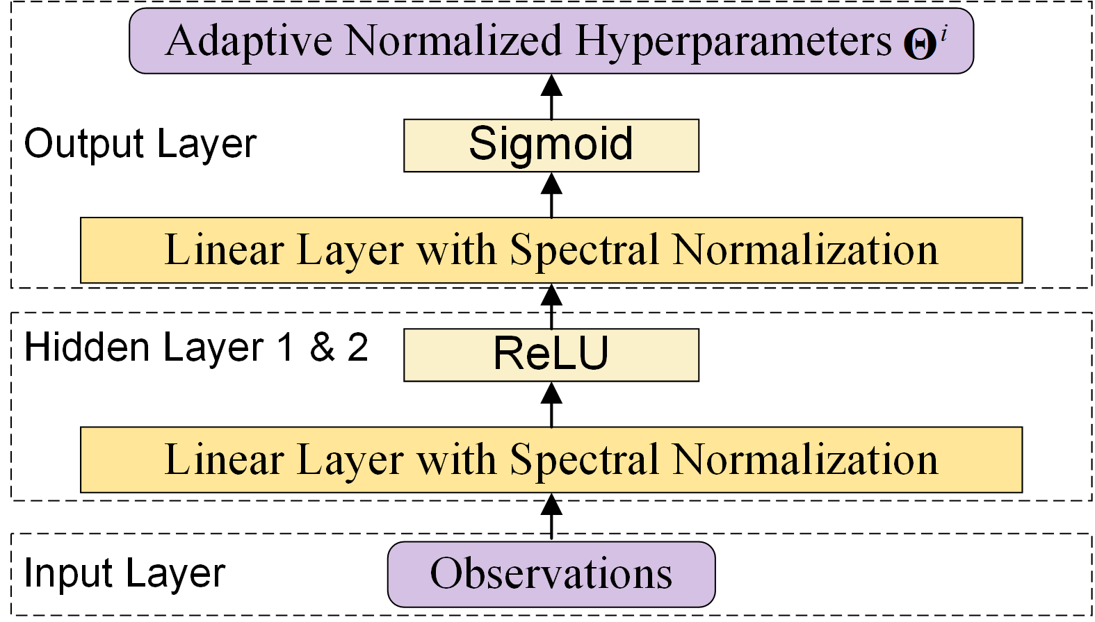
Figure 3: Architecture of the neural network for producing the adaptive MPC normalized hyperparameters $\bm{\Theta}^{i}$ online. As the network’s input, the observations can include the system tracking errors or obstacle information, depending on the applications.

To reflect the above parameterization, the chain rule (15) for the gradient computation is therefore rewritten as:

$$\frac{dL^{i}}{d\bm{\varpi}^{i}}=\frac{\partial L^{i}}{\partial X_{\mathrm{cl}}^{i}}\frac{\partial X_{\mathrm{cl}}^{i}}{\partial\bm{\theta}^{i}}\frac{\partial\bm{\theta}^{i}}{\partial\bm{\Theta}^{i}}\frac{\partial\bm{\Theta}^{i}}{\partial\bm{\varpi}^{i}},\ \forall i\in\mathcal{I}_{A}.$$ (32)

We implement our method in Python and solve the distributed MPC problems described in Algorithm 1 using ipopt via CasADi [43]. The MLP, illustrated in Fig. 3, is built using PyTorch [44] and trained using Adam [45]. During the implementation, we customize the loss function $L^{i}$, which can be (28) or (29), or a combination of both, to align with the typical training procedure in PyTorch. Specifically, the customized loss function for training the network is defined as $L_{{\rm{pytorch}}}^{i}={\left.{\frac{{d{L^{i}}}}{{d{{\bm{\Theta}}^{i}}}}}\right|_{{\bm{\Theta}}_{t}^{i}}}{{\bm{\Theta}}^{i}}$. Here ${\left.{\frac{{d{L^{i}}}}{{d{{{\bm{\Theta}}}^{i}}}}}\right|_{{{\bm{\Theta}}}_{t}^{i}}}={\left.{\frac{{\partial{L^{i}}}}{{\partial X_{{\rm{cl}}}^{i}}}}\right|_{X_{{\rm{cl,}}t}^{i}}}{\left.{\frac{{\partial X_{{\rm{cl}}}^{i}}}{{\partial{\bm{\theta}^{i}}}}}\right|_{\bm{\theta}_{t}^{i}}}{\left.{\frac{{\partial{\bm{\theta}^{i}}}}{{\partial{\bm{\Theta}^{i}}}}}\right|_{\bm{\Theta}_{t}^{i}}}$ represents the gradient of $L^{i}$ w.r.t. $\bm{\Theta}^{i}$ evaluated at $\bm{\Theta}_{t}^{i}$. This ensures that $\frac{dL_{\mathrm{pytorch}}^{i}}{d\bm{\varpi}^{i}}=\frac{dL^{i}}{d\bm{\varpi}^{i}}$.

VI-A Distributed Learning of Adaptive Weightings

We design a trajectory tracking flight scenario to demonstrate the first and second advantages of our method. We consider a challenging multilift system with a non-uniform load mass distribution, resulting in a biased load CoM coordinate within its body frame. In this simulation, the load CoM coordinate is set to ${\bm{r}}^{g}=\left[0.1,0.1,-0.1\right]\ {\rm m}$. Under these conditions, balancing the load during flight requires uneven and dynamic tension allocation among the quadrotors, making manual selection of the MPC weightings extremely difficult. Assuming no obstacles during flight, we focus on learning adaptive MPC weightings that enable the multilift system to track the reference trajectory while stabilizing the load’s attitude. To this end, the individual loss function $L^{i}$ is defined using (28). We plan circular reference trajectories for each agent using the minimum snap algorithm [40], based on a fixed system configuration. To reduce the network size, we constrain the MPC weighting matrices to be diagonal, resulting in a total of $28$ weightings for each quadrotor and $24+n$ weightings for the load (where $n$ is the number of quadrotors). We set the number of neurons in the hidden layer to $30$ and take the tracking errors as input. Finally, the lower and upper bounds for the adaptive MPC weightings are set to $0.01$ and $100$, respectively.

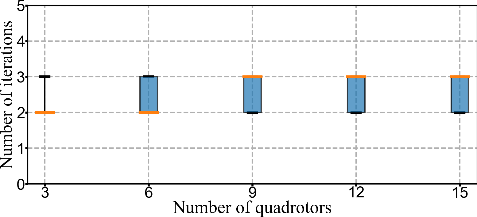
Figure 4: Boxplot of the number of iterations required for DSP convergence. The data are collected by running Algorithm 2 $300$ times during training with $\delta=10^{-4}$ and $k_{\max}=5$.

Before demonstrating the learning performance of Auto-Multilift, we first assess its convergence properties by measuring the number of iterations required for the DSP algorithm to converge. In Fig. 4, we present boxplots of the number of iterations across different number of quadrotors used in the multilift system. Although the DSP requires one more iteration to converge when the number of quadrotors increases from $6$ to $9$, the convergence speed stabilizes at three iterations, regardless of any further increases in the number of quadrotors. This shows the fast convergence advantage of the proposed algorithm.

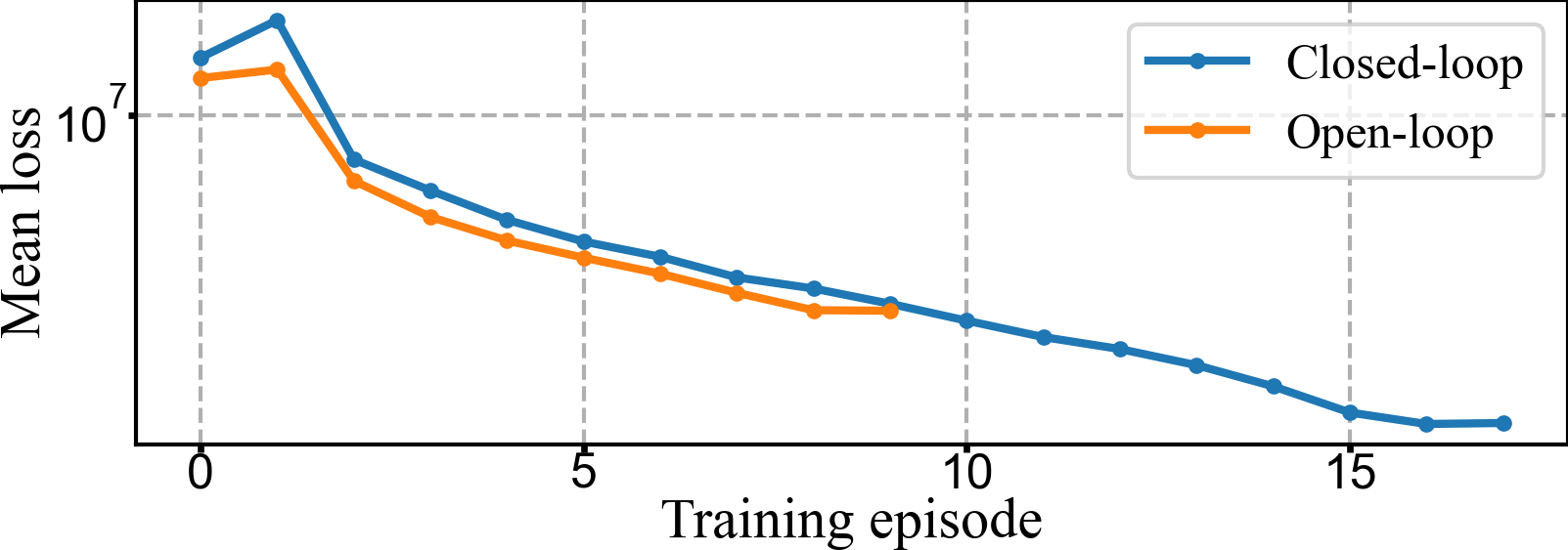
(a) Comparison of the mean loss with three quadrotors.

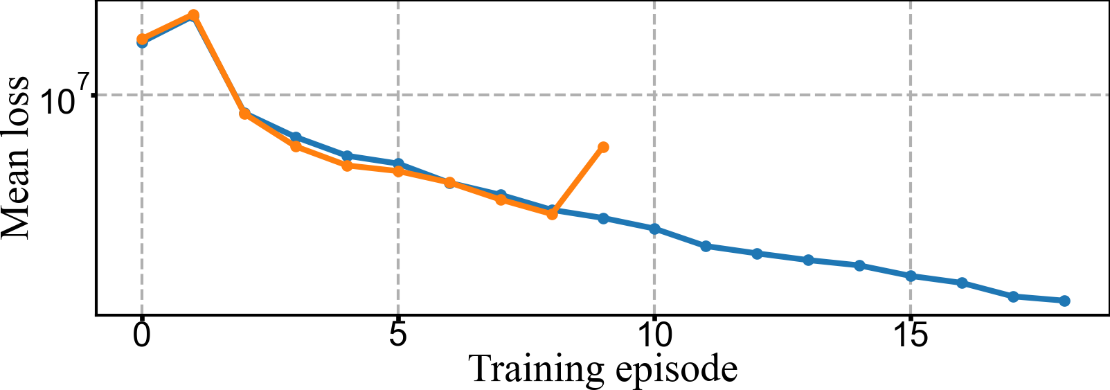
(b) Comparison of the mean loss with six quadrotors.

Figure 5: Comparison of the mean loss between the closed-loop method (as outlined in Algorithm 3) and the open-loop method [24]. These two training methods are implemented using the same stop criterion. Specifically, the training will stop when $\left|L_{\mathrm{mean}}^{k}-L_{\mathrm{mean}}^{k-1}\right|\leq\frac{1}{1000}L_{\mathrm{mean}}^{0},\ \forall k\geq 1$, where $L_{\mathrm{mean}}^{k}$ denotes the mean loss at iteration $k$. Note that the open-loop training with six quadrotors is divergent, and the extremely large mean loss value after episode $9$ has been removed from the figure for clearer illustration.

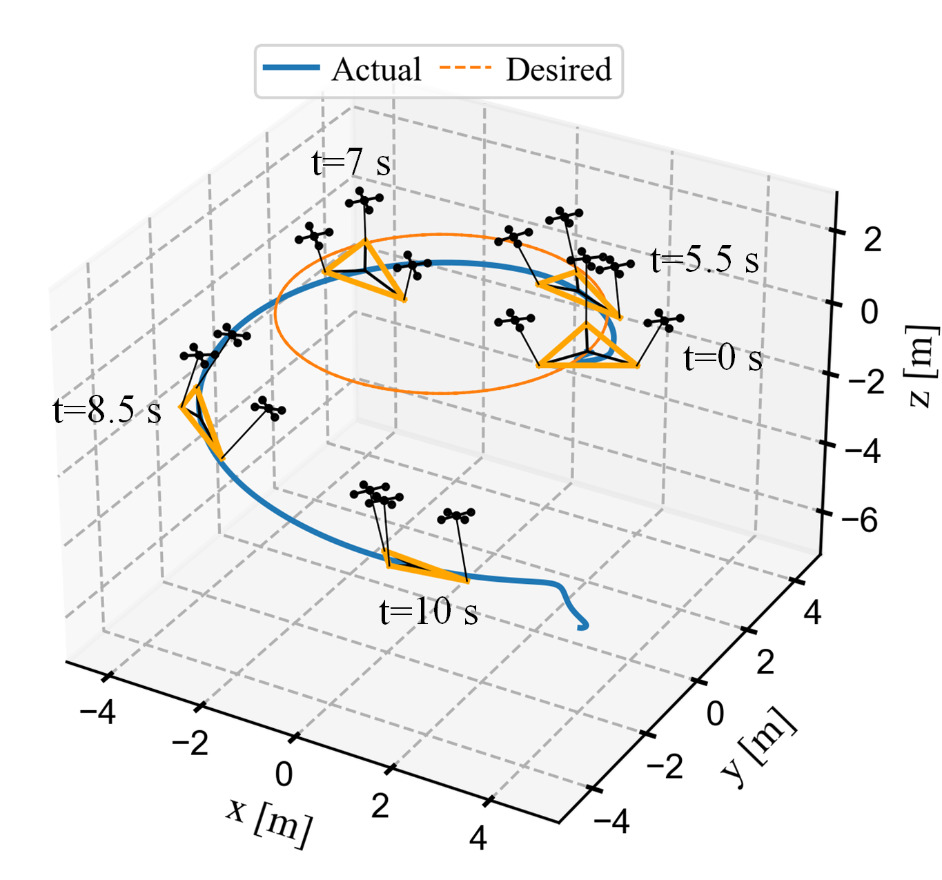
(a) Episode $0$ with three quadrotors.

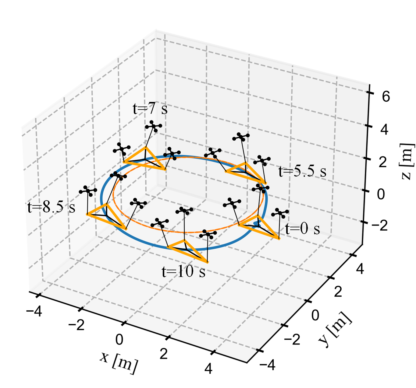
(b) Episode $9$ with three quadrotors.

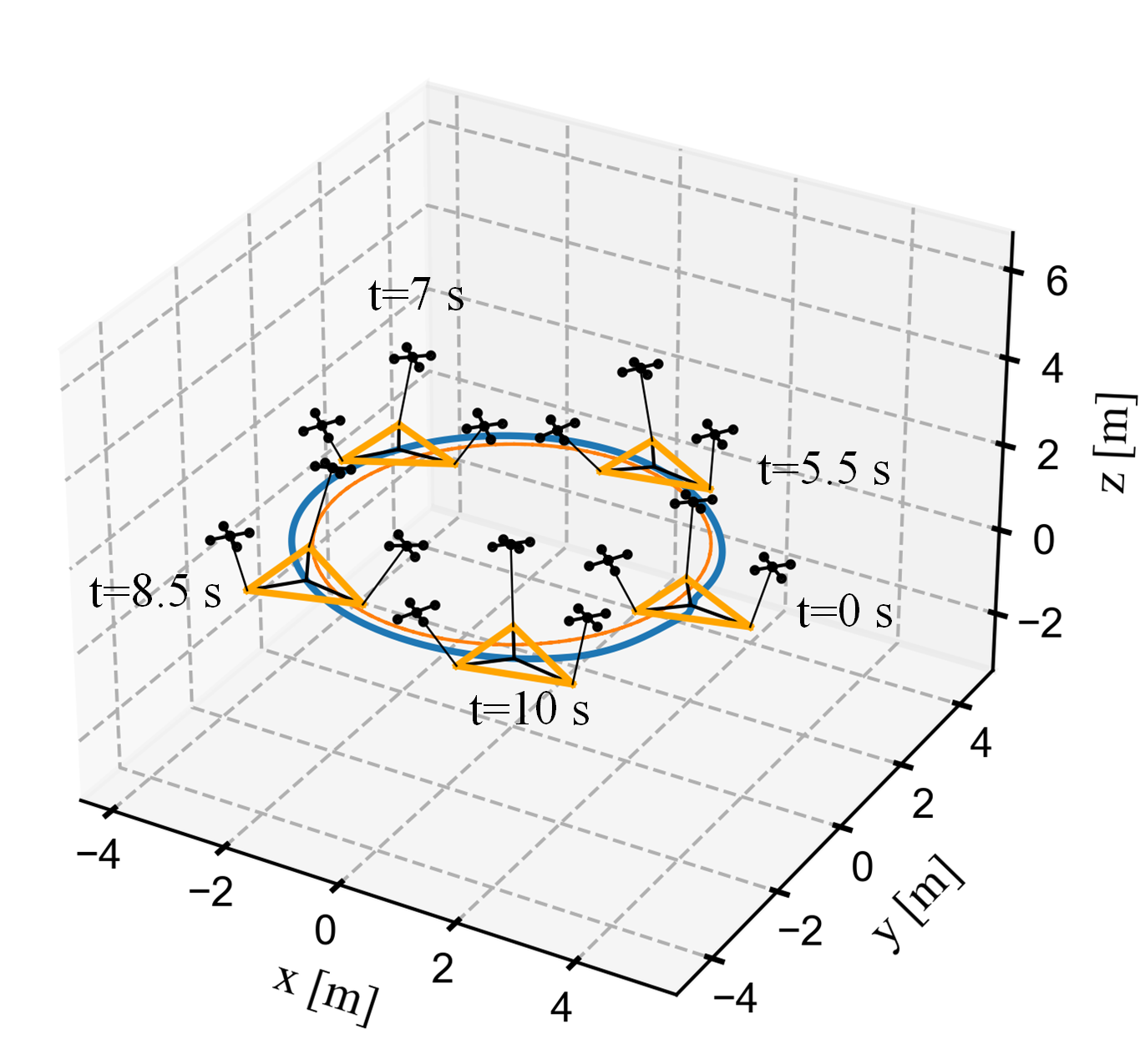
(c) Episode $17$ with three quadrotors.

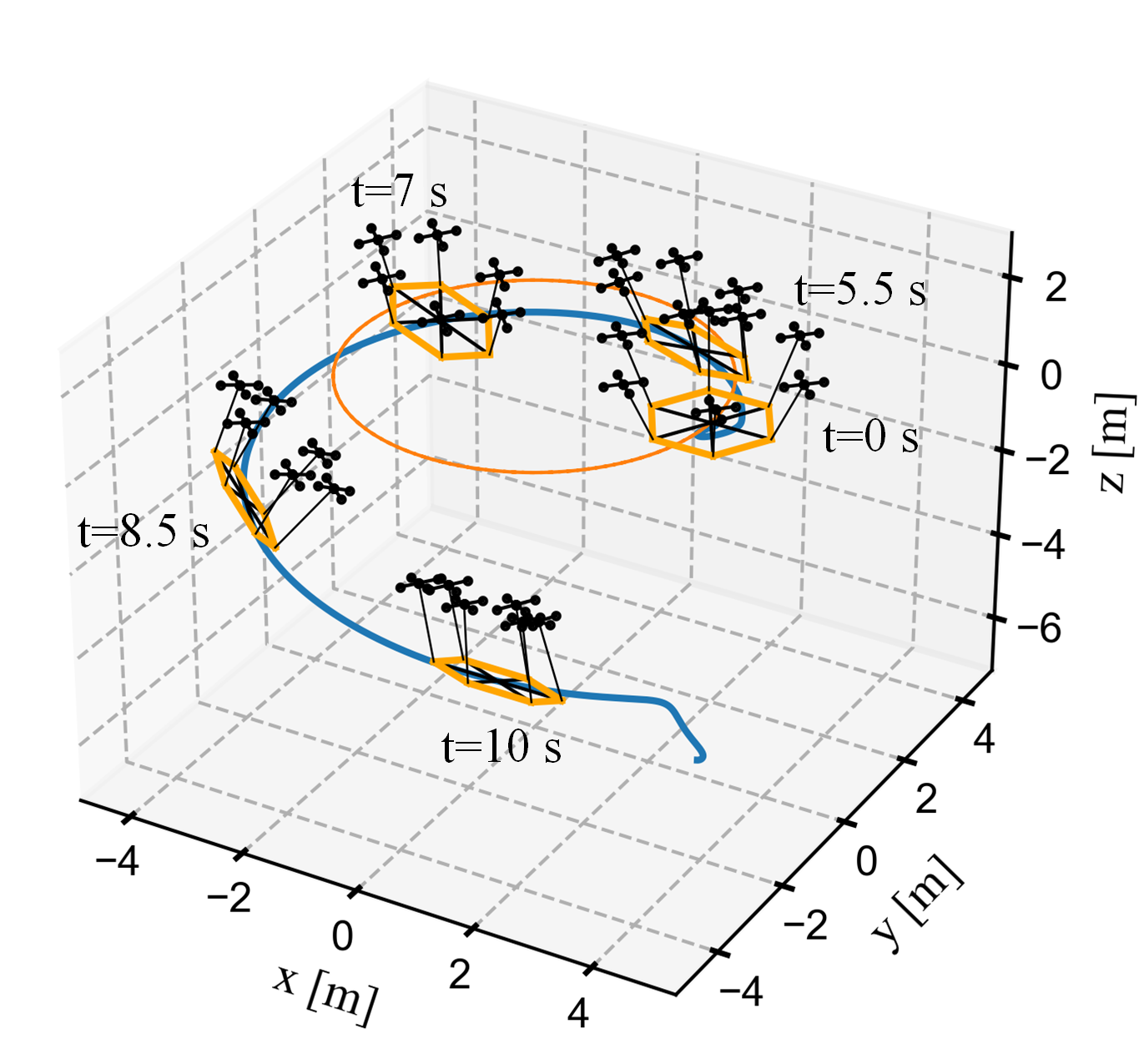
(d) Episode $0$ with six quadrotors.

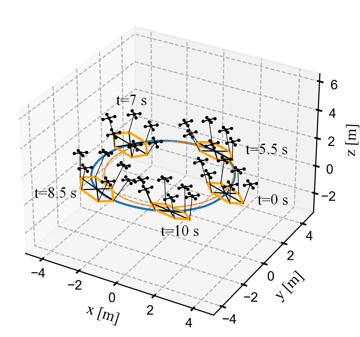
(e) Episode $9$ with six quadrotors.

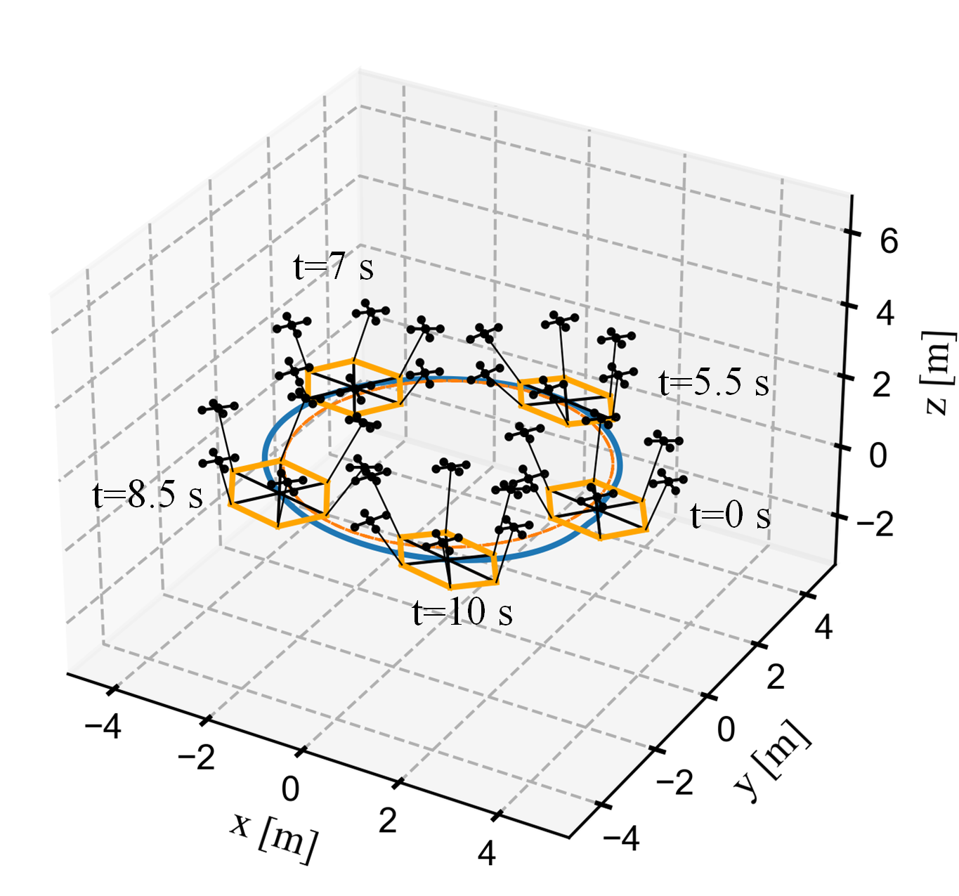
(f) Episode $17$ with six quadrotors.

Figure 6: 3D Illustrations of the learning process of Auto-Multilift via Algorithm 3 with three and six quadrotors. The planned flight duration for the circular reference trajectory is $15$ seconds, and we display $5$ instants at $t=0\ {\rm s}$, $t=5.5\ {\rm s}$, $t=7\ {\rm s}$, $t=8.5\ {\rm s}$, and $t=10\ {\rm s}$, respectively.

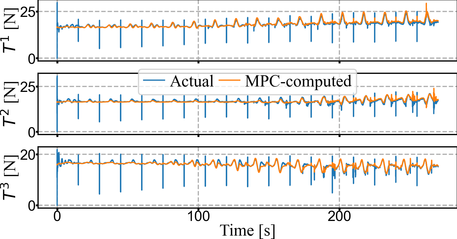
Figure 7: Comparison of the actual and the MPC-computed tension magnitudes with three quadrotors during the proposed closed-loop training. Due to the non-uniform mass distribution of the load, the tension allocation among three quadrotors is unequal and dynamic.

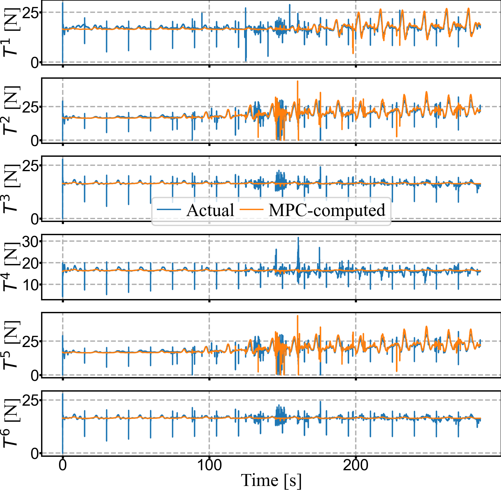
Figure 8: Comparison of the actual and the MPC-computed tension magnitudes with six quadrotors during the proposed closed-loop training. Compared with the case in Fig. 7, the tension allocation among six quadrotors is more dynamic.

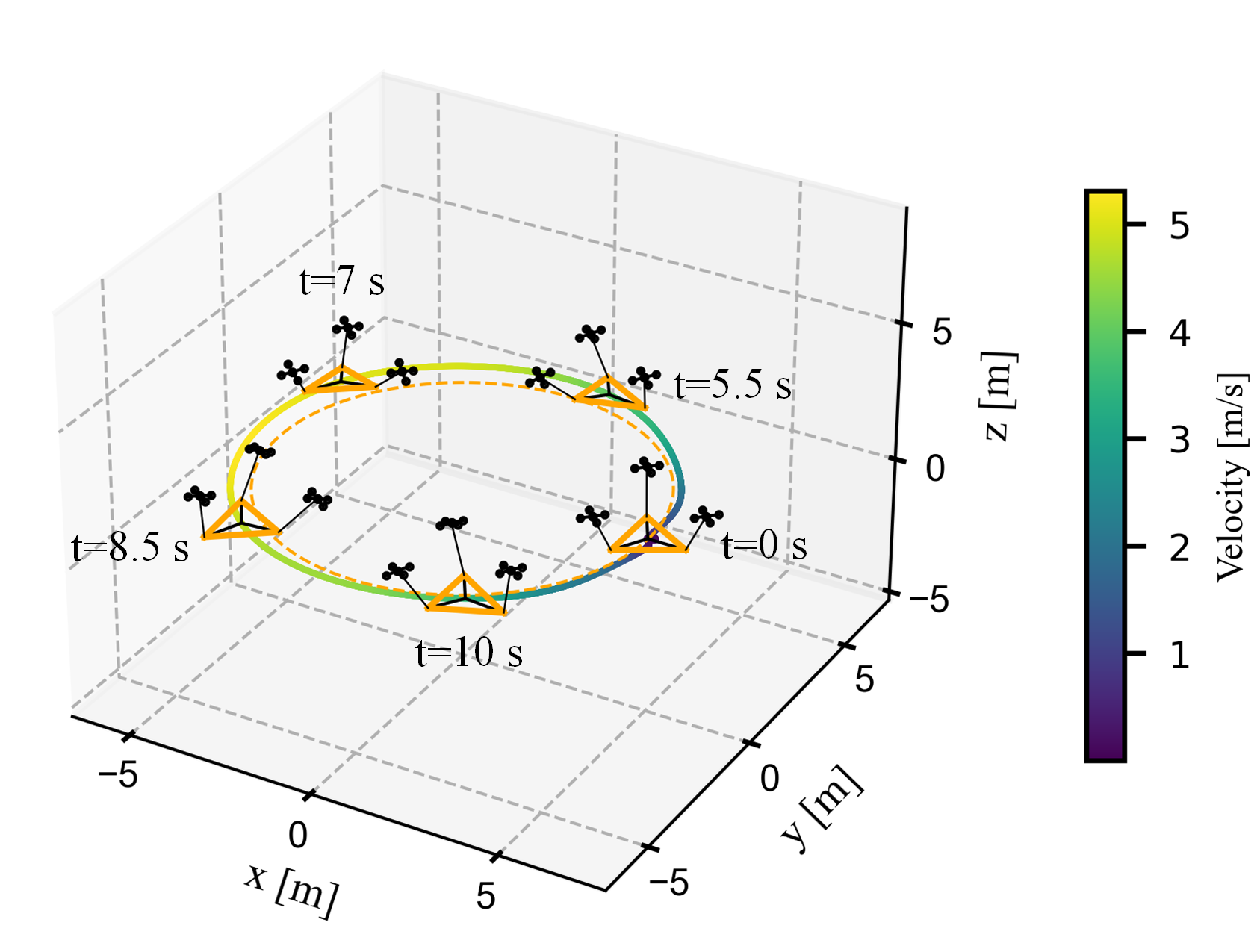
(a) Three quadrotors trained using Algorithm 3.

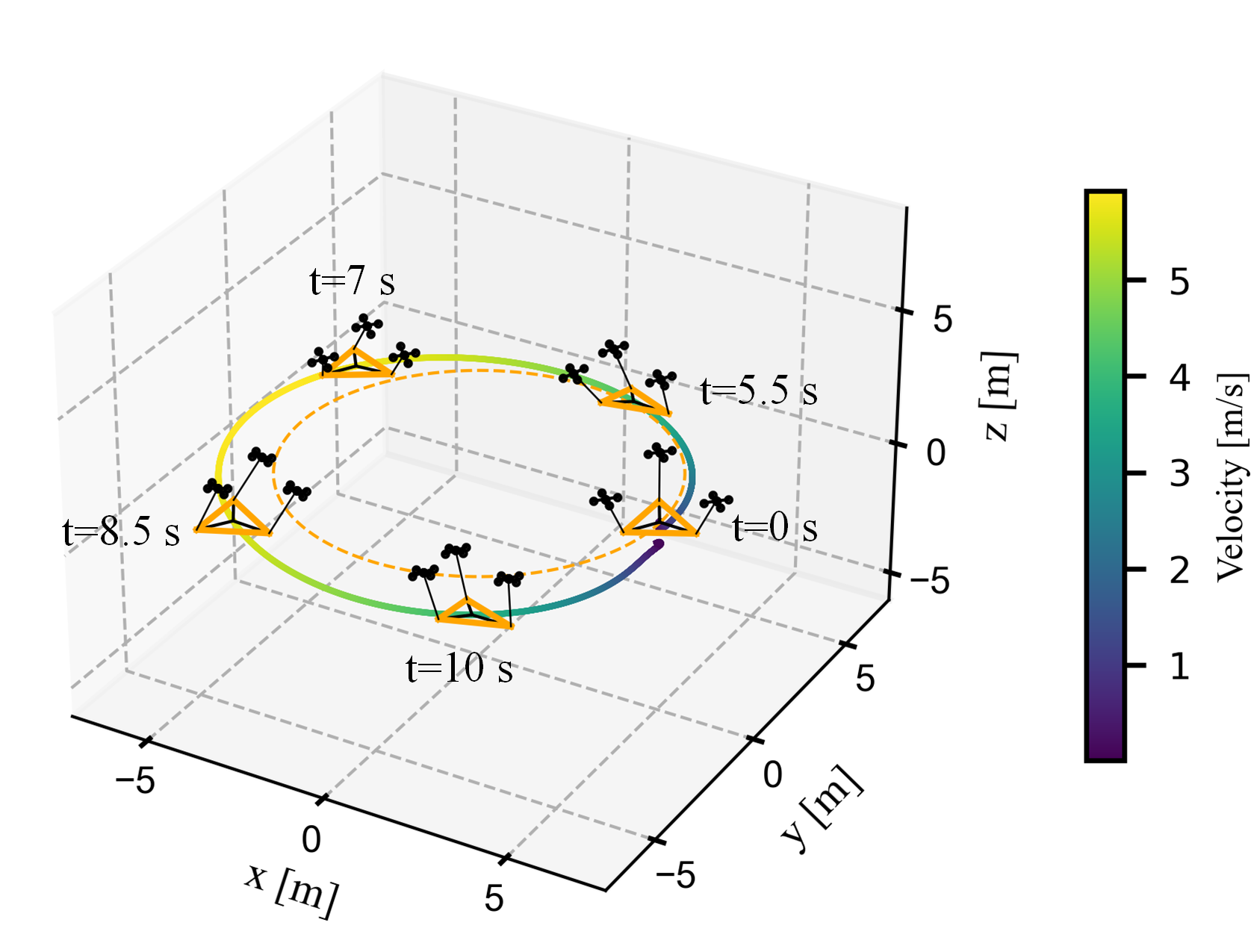
(b) Three quadrotors trained using the open-loop method [24].

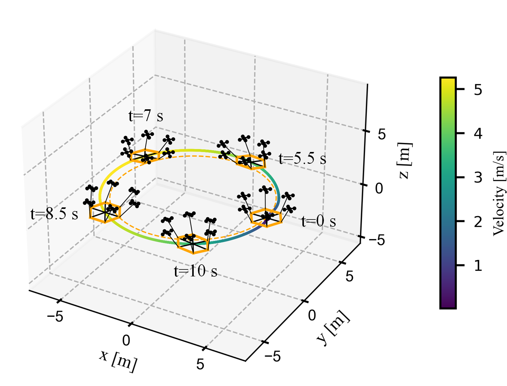
(c) Six quadrotors trained using Algorithm 3.

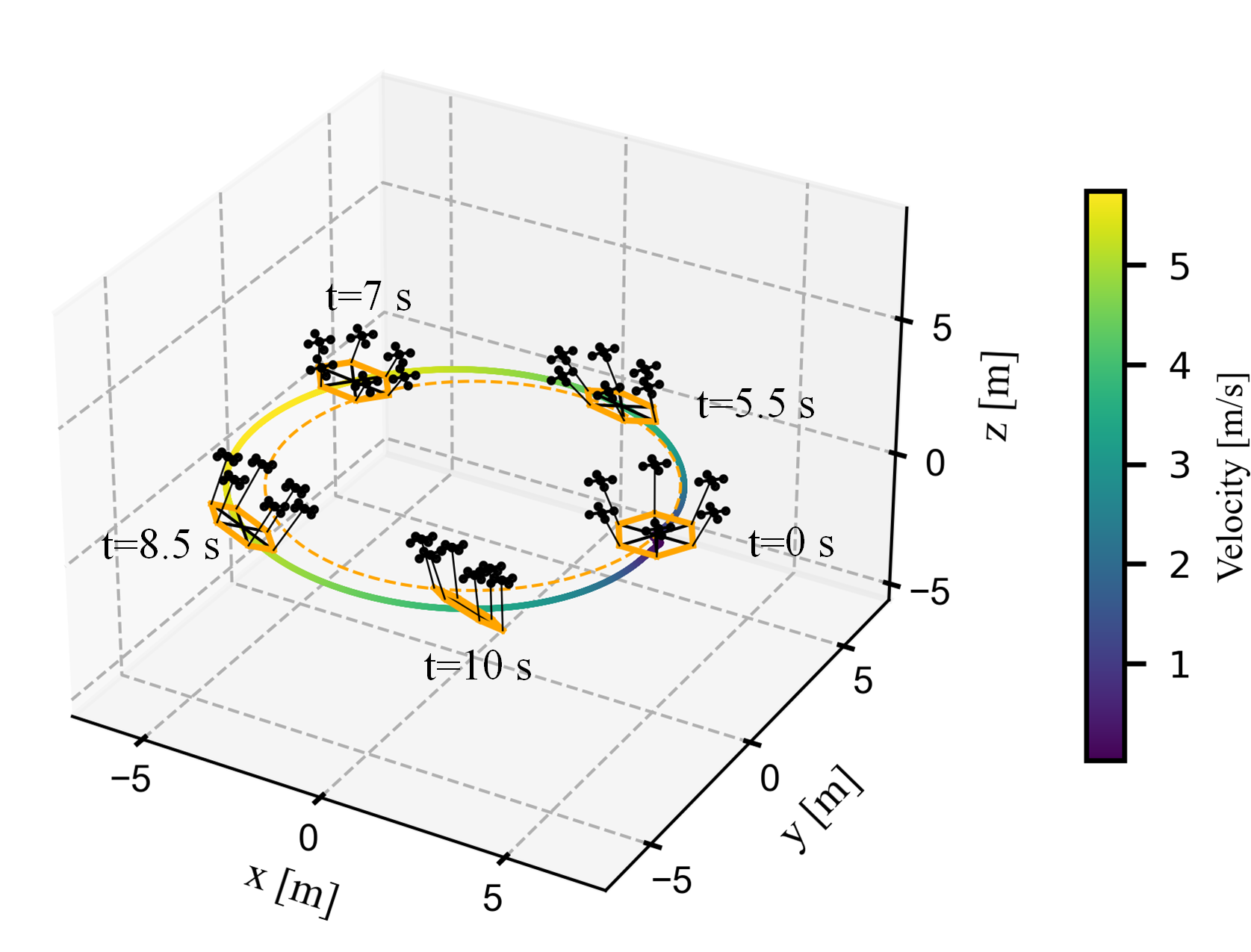
(d) Six quadrotors trained using the open-loop method [24] through episode $9$.

Figure 9: 3D Illustrations of the evaluation results on an unseen circular trajectory. Compared with the slower trajectory used in training, we halve the load masses of these two multilift systems. This reduction ensures sufficient thrust margins to accommodate the larger accelerations required by the more agile test trajectory, addressing stability concerns.

We then validate the learning capability of our method using two multilift systems: one with three quadrotors transporting a $5\ {\mathrm{kg}}$ load, and another with six quadrotors transporting a heavier $10\ {\mathrm{kg}}$ load. In the first case, we need to train a total of four networks (three for the quadrotors and one for the load), while in the second case, a total of seven networks are to be trained. To highlight the important role that the DSP plays in our method, we conduct an ablation study by comparing it with the state-of-the-art open-loop training method, Safe-PDP [24]. In training, we set $N=10$ as the MPC horizon for open-loop prediction and $N_{\mathrm{cl}}=20$ as the loss horizon for closed-loop training. The distributed MPC problems (10) and (11) are solved using Algorithm 1 in a receding horizon manner. One training episode involves training these networks for each agent in parallel over their $15$-s-long circular reference trajectories once (i.e., $T_{\mathrm{ep}}=15\ {\rm{s}}$ in Algorithm 3). When strictly aligning with the open-loop training method in [24], one can only implement Algorithm 1 once per episode. In that case, an extremely long MPC horizon is required to cover the whole trajectory, which is computationally expensive and often infeasible. Given this limitation, in the open-loop training for the ablation study, we continue to implement Algorithm 1 in a receding horizon manner, as done in the closed-loop training, and solve Problem (14) using the Safe-PDP method with $N_{\mathrm{ol}}=10$. Note that in (14), the individual losses are based on their respective open-loop prediction trajectories from the MPCs.

Fig. 5 compares the mean loss during training between our method and the Safe-PDP open-loop training method for these two multilift systems. For a fair comparison, all the mean losses shown in the figure are computed using the same loss function (28), based on the closed-loop system states. Despite the closed-loop implementation of the MPCs, Fig. 5(a) shows that the mean loss of the Safe-PDP method stabilizes at a significantly higher value, indicating poorer trajectory tracking performance. For the larger multilift system with a heavier load, the Safe-PDP method even leads to unstable training, with the mean loss trajectory showing divergence (see Fig. 5(b)). In contrast, our method’s mean loss trajectories can stabilize at much smaller values for both the multilift systems, exhibiting the advantages of stable learning and better tracking performance. Fig. 6 visualizes the training process using 3D plots. In both cases, our method improves the tracking performance over training episodes while gradually stabilizing the load’s attitude in the desired horizontal direction.

Our method’s advantages over the Safe-PDP method stem from two main factors. First, we train directly on the closed-loop system states from the actual system dynamics, whereas the Safe-PDP method relies on the open-loop predicted states from the nominal system dynamics. This distinction is critical since it addresses the discrepancies between the actual and the MPC-computed tensions, as shown in Figs. 7 and 8. The MPC-computed tensions are substantially smoother than the actual tensions. Although both methods use $\mathcal{L}_{1}$ adaptive control [39] to robustify the MPCs against these differences, training on the closed-loop data provides a more robust and effective means to improve tracking performance. A notable example is during episode $9$ of training the large multilift system, from $135\ {\rm s}$ to $150\ {\rm s}$ in Fig. 8. Despite high-frequency fluctuations in the actual tensions, our method effectively computes appropriate gradients to stabilize training, whereas the Safe-PDP method leads to instability. Second, our method permits a longer loss horizon than the MPC horizon. This results in gradients that contain richer information for training compared to open-loop methods like Safe-PDP.

TABLE II: Comparisons of Load Tracking Errors (RMSE)

[t] Method ${p_{x}}$ ${p_{y}}$ ${p_{z}}$ Roll Pitch Yaw $\left[{\rm m}\right]$ $\left[{\rm m}\right]$ $\left[{\rm m}\right]$ $\left[{\rm deg}\right]$ $\left[{\rm deg}\right]$ $\left[{\rm deg}\right]$ Safe-PDP $(3)$ $0.47$ $0.50$ $0.48$ $12.15$ $\bf 3.16$ $3.98$ Our method $(3)$ ${\bf 0.25}$ ${\bf 0.25}$ ${\bf 0.13}$ ${\bf 4.88}$ ${4.70}$ ${\bf 1.29}$ Safe-PDP $(6)$ $0.36$ $0.39$ $0.16$ $24.28$ $16.42$ $9.93$ Our method $(6)$ ${\bf 0.26}$ ${\bf 0.27}$ ${\bf 0.10}$ $\bf 5.36$ ${\bf 4.78}$ ${\bf 1.41}$

• $(3)$ and $(6)$ represent three and six quadrotors, respectively.

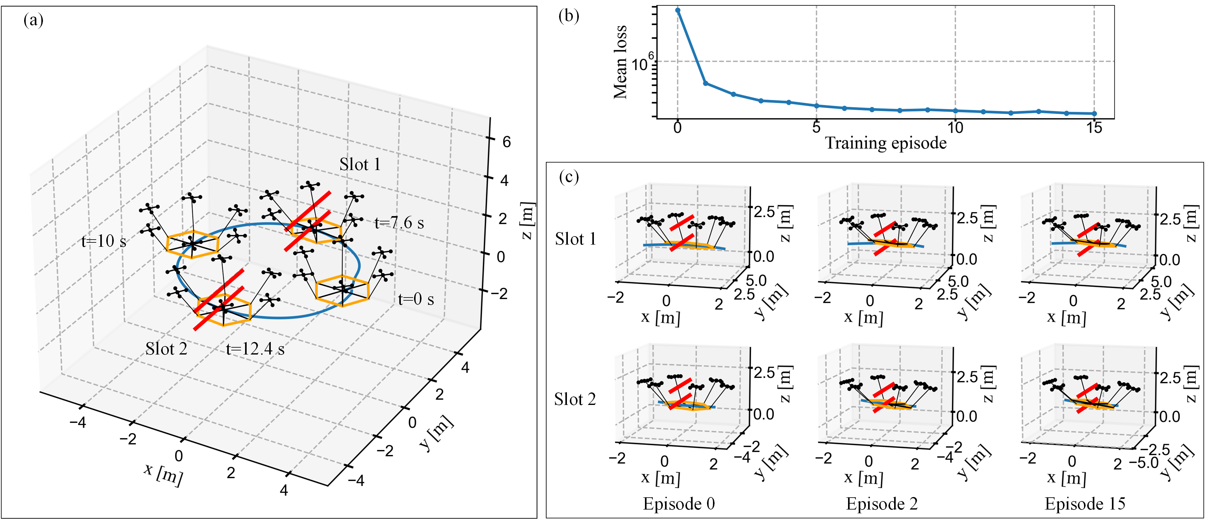
Figure 10: Illustrations of the process of learning the tension reference using Algorithm 3. (a) 3D plot showing the positions of two slots on a circular trajectory, with slot 2 being $0.15\ {\rm m}$ shorter in height than slot 1. (b) The changing pattern of mean loss during training. (c) 3D plots showing the learning process of the large multilift system when passing through these two slots.

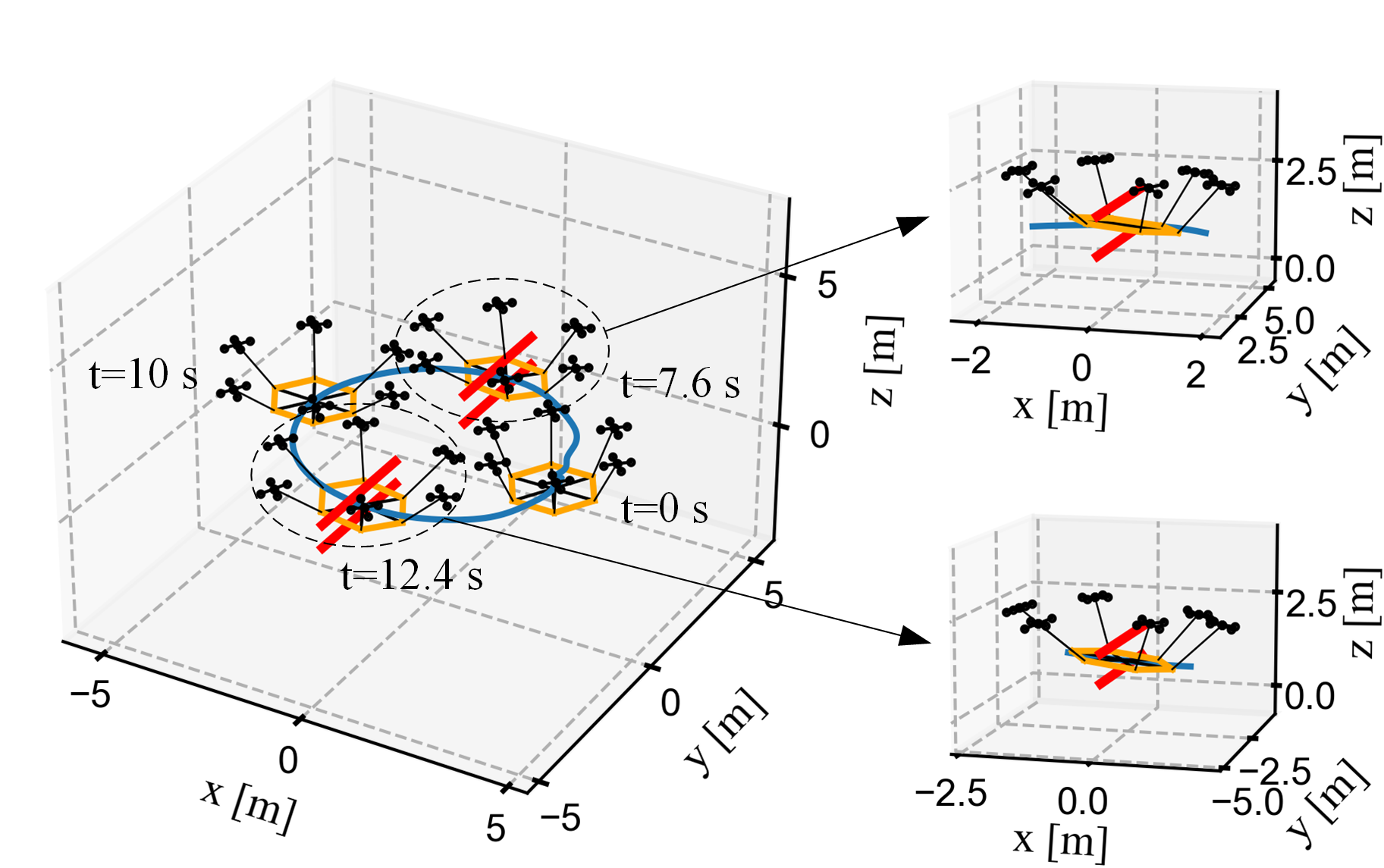
(a) Passing through slots with the tension compensation on.

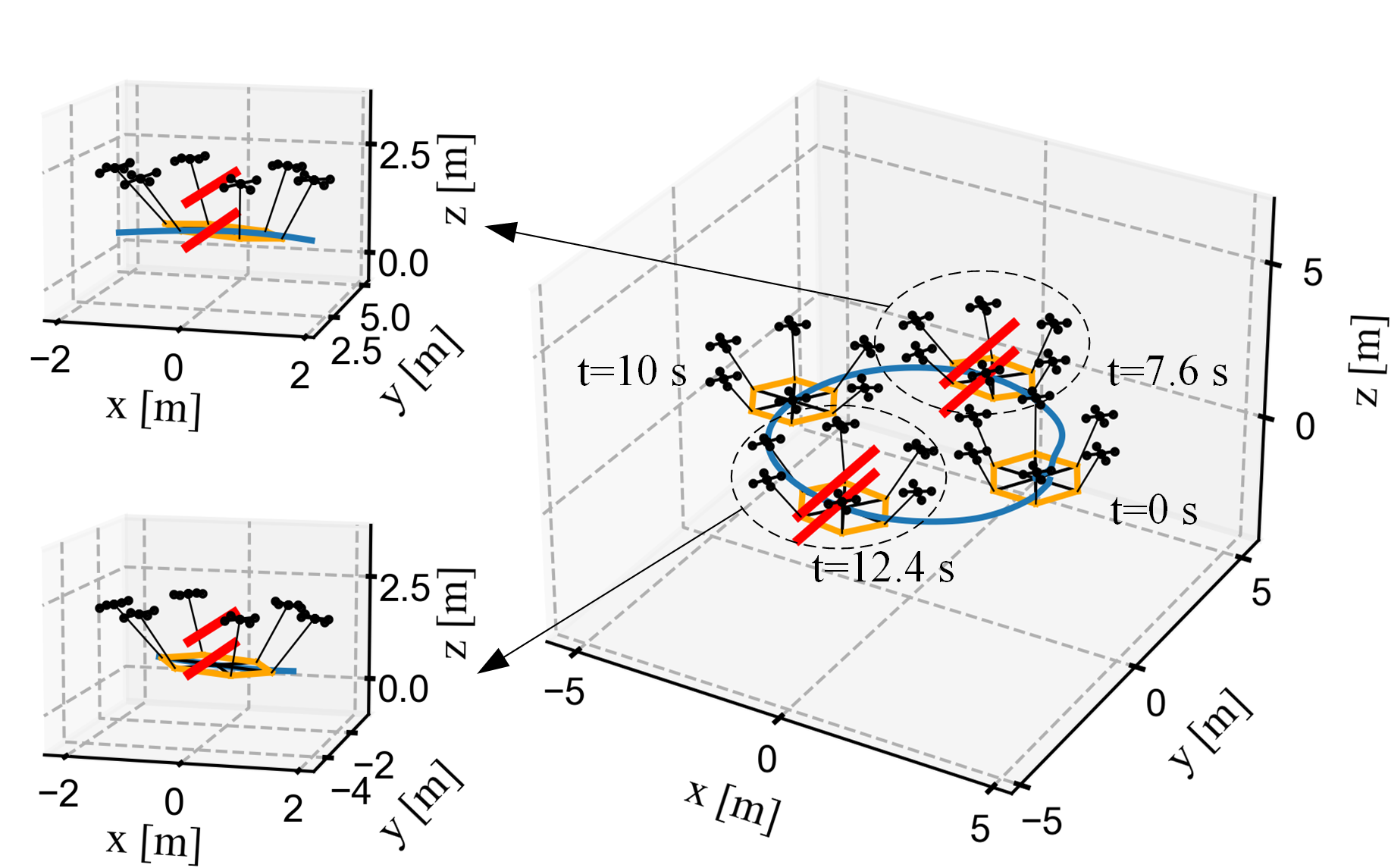
(b) Colliding with slots when the tension compensation is off.

Figure 11: 3D comparison of the large multilift system passing through the slots, with and without the tension reference compensation.

In evaluation, we compare the tracking performance between our method and Safe-PDP on a previously unseen circular trajectory with a larger radius ($r=5\ {\rm m}$) than the training trajectory ($r=3\ {\rm m}$), both having the same duration, which necessitates more agile maneuvers. Fig. 9 illustrates this comparison using 3D plots. Our method achieves smaller tracking errors and brings the load’s attitude closer to horizontal than Safe-PDP. We quantify the tracking performance using the root-mean-square errors (RMSEs) and summarize the comparison in Table II. Notably, Auto-Multilift exhibits significantly smaller RMSEs in all directions compared to Safe-PDP, improving the accuracies of trajectory tracking and load attitude stabilization by up to $72\%$ and $78\%$, respectively. The only exception is in the pitch angle for the smaller multilift system, where our method exhibits a slightly larger RMSE than Safe-PDP.

VI-B Distributed Learning of Adaptive References

To demonstrate the third advantage of our method, we design an obstacle avoidance flight scenario. Specifically, the large multilift system, equipped with six quadrotors and trained using our method in subsection VI-A, is required to pass through two slots. As shown in Fig. 10(a), these two slots are symmetrically positioned on a circular trajectory and have their heights shorter than the cable length of $1.5\ {\rm m}$. Successfully passing through confined spaces like these slots is a crucial capability for multilift systems, especially in applications like rescue operations. In this scenario, the quadrotors must spread apart to pass through and then gather together afterward.

These dynamic configuration changes pose significant challenges to the design of reference trajectories for multilift systems. To simplify the problem, we consider a dynamic configuration based on the following adaptive cable tilt angle:

$$\beta_{t}=\beta_{\min}+\left(\beta_{\max}-\beta_{\min}\right)\mathrm{exp}\left(-\eta_{\mathrm{cf}}\left\|{\bm{p}}_{t}^{l}-{\bm{p}}^{\mathrm{s}}\right\|_{2}\right)$$ (33)

where $\beta_{\min}$ and $\beta_{\max}$ represent the lower and upper bounds, respectively, $\beta_{\max}$ is determined using the geometric relationship between the cable length and the slot height, ${\bm{p}}^{\mathrm{s}}$ denotes the slot’s position in the world frame, and $\eta_{\mathrm{cf}}\in\mathbb{R}_{+}$ is a positive coefficient. This tilt angle applies to all the cables. Compared with $\beta_{t}$, designing the tension reference is more challenging. Note that the tension references from the static configuration in subsection VI-A are not sufficient to ensure collision avoidance while passing through the slots. This is because the tension reference must be adjusted dynamically when the configuration changes, guiding the load’s MPC to generate appropriate tensions that maintain the load’s height above the lower boundary of the slot. To achieve this, we aim to learn such an adaptive tension reference using Algorithm 3. The adaptive tension reference acts as a tension compensation $\Delta T^{\mathrm{ref}}\in\mathbb{R}$ added to the tension reference employed in subsection VI-A, and applies to all the cables. It is modeled by an $8$th network for the large multilift system, which takes as inputs the height and vertical velocity tracking errors, along with the dynamic tilt angle $\beta_{t}$. We define the training loss by combining (28) and (29) as follows:

$$L^{l}=\alpha\sum_{t=T}^{T+N_{\mathrm{cl}}}\left[\left(1-\alpha_{t}^{\mathrm{s}}\right)\left(z_{t}^{l}-z_{t}^{l,\mathrm{ref}}\right)+\alpha_{t}^{\mathrm{s}}\mathrm{exp}\left(-\eta\left(z_{t}^{l}-z^{\mathrm{s}}\right)\right)\right]$$ (34)

where $\alpha_{t}^{\mathrm{s}}=\mathrm{exp}\left(-\eta^{\mathrm{s}}\left\|{\bm{p}}_{t}^{l}-{\bm{p}}^{\mathrm{s}}\right\|_{2}\right)$, $\eta^{\mathrm{s}}\in\mathbb{R}_{+}$ is a positive coefficient, $z_{t}^{l}$ is the load’s actual height, $z_{t}^{l,\mathrm{ref}}$ is the reference height from the reference circular trajectory, and $z^{\mathrm{s}}$ denotes the height of the slot’s lower boundary.

Fig. 10(b) shows the stable mean loss decreasing over the learning episodes. Fig. 10(c) visualizes the learning process via 3D plots, focusing on the traversing stage. During training, our method gradually increases the load’s height when passing through the slots and finally lifts it above the lower boundaries of the slots at episode 15, achieving collision-free passage.

In evaluation, we reduce the heights of slot 1 and 2 by $0.1\ {\rm m}$ and $0.15\ {\rm m}$, respectively. This requires larger $\beta_{t}$ to pass through the slots compared to the training phase, posing a more significant challenge to the tension compensation $\Delta T^{\mathrm{ref}}$. Fig. 11 compares the collision avoidance performance of the large multilift system when passing through the slots, with and without $\Delta T^{\mathrm{ref}}$. Comparing the zoom-in plots in Fig. 11(a) and 11(b) shows that the tension compensation is of great importance for avoiding collisions with the lower boundaries. This occurs because, with the compensation, the actual tensions in these six cables increase appropriately during the two passing stages, compared to those without the compensation, as illustrated in Fig. 12.

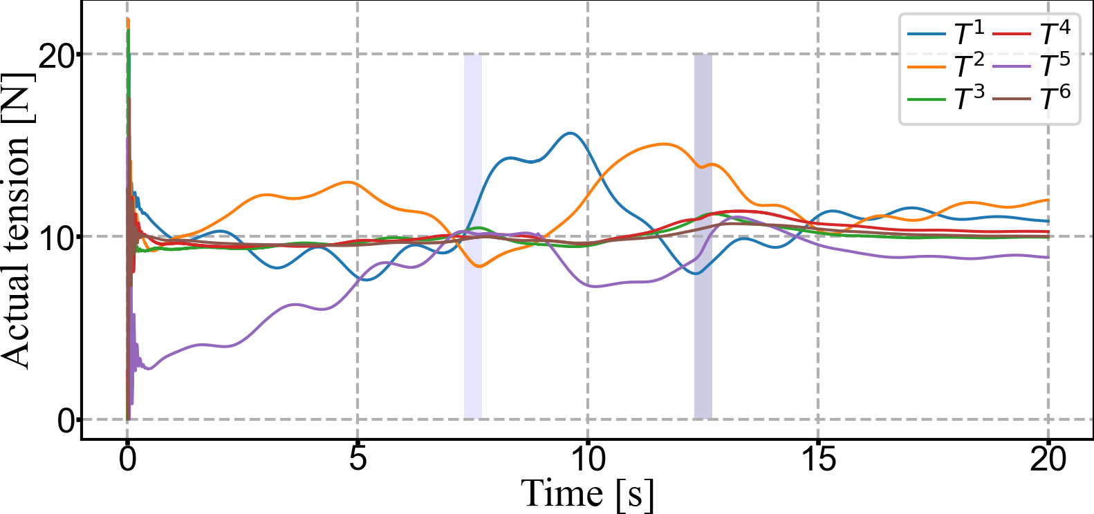
(a) Actual tensions with the compensation on

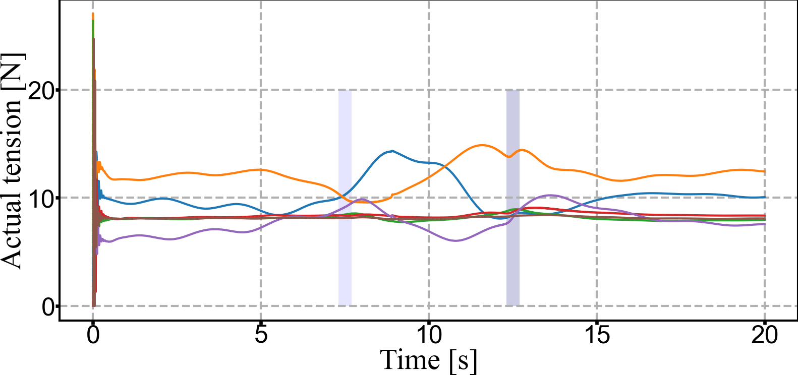
(b) Actual tensions when the compensation is off.

Figure 12: Comparisons of the actual cable tensions, with and without the tension compensation. The left and right shadow blocks represent the first and second passing stages, respectively.

VII Discussion

Auto-Multilift features a distributed and closed-loop learning framework, which efficiently trains adaptive higher-level policies (i.e., the hyperparameters modeled by DNNs) via RL for the distributed MPCs of the multilift system. Our method enjoys fast convergence and can be applied to learn various MPC hyperparameters. In addition, it outperforms the state-of-the-art open-loop training method Safe-PDP in terms of learning stability and trajectory tracking performance.

On the other hand, Auto-Multilift can be further improved in the following aspects. Although the proposed DSP algorithm achieves fast convergence in just a few iterations, the computation time for the distributed MPCs (implemented via Algorithm 1) is relatively long due to the high nonlinearity of the multilift system dynamics. To reduce this time for real-world flight, optimized numerical solvers and code structures would be needed. Another limitation is that the stability of nonlinear distributed MPCs and neural network-based controllers remains an open problem. Although a theoretical analysis of the stability may prove difficult, one could explore and extend the boundaries of this stability using meta-learning with curriculum training strategies.

VIII Conclusion

This paper proposed a novel learning framework, Auto-Multilift, for cooperative cable-suspended load transportation with quadrotors. Our critical insight is that Auto-Multilift can automatically tune various adaptive MPC hyperparameters, which are modeled by DNNs and difficult to tune manually, via RL in a distributed and closed-loop manner. At the core of our method is the distributed sensitivity propagation algorithm, which efficiently computes the sensitivities of the closed-loop states w.r.t. the MPC hyperparameters and can converge in finite iterations with theoretical guarantees. We have shown through extensive simulations that our method features fast convergence, good scalability to large multilift systems, and improved learning stability and tracking performance over the state-of-the-art open-loop training method.

Our future work involves further enhancing the training method of Auto-Multilift via meta-learning and conducting real-world flight experiments to validate its online learning performance in real-time.

-A Coefficient Matrices for the Load’s MPC Problem

We introduce $\bar{\bm{\theta}}^{l}$ as the generalized hyperparameters for the load’s MPC problem (11), which can denote ${\bm{x}}_{t}^{l}$, ${\bm{x}}_{0|t}^{\ast,i}\left(\forall i\in\mathcal{I}_{q}\right)$, or $\bm{\theta}^{l}$. The corresponding matrices are defined as follows:

$$\mathbf{H}_{k}^{u\bar{\theta}} =\frac{\partial^{2}H_{k}^{l}}{\partial{\bm{u}}_{k|t}^{\ast,l}\partial\bar{\bm{\theta}}^{l}},\mathbf{E}_{k}=\frac{\partial\bar{\bm{f}}_{k}^{l}}{\partial\bar{\bm{\theta}}^{l}},\frac{\partial{\bm{x}}_{0|t}^{\ast,l}}{\partial\bar{\bm{\theta}}^{l}}=\frac{\partial{\bm{x}}_{t}^{l}}{\partial\bar{\bm{\theta}}^{l}},$$ (35)

$$\mathbf{H}_{k}^{x\bar{\theta}} =\frac{\partial^{2}H_{k}^{l}}{\partial{\bm{x}}_{k|t}^{\ast,l}\partial\bar{\bm{\theta}}^{l}},\mathbf{H}_{N}^{x\bar{\theta}}=\frac{\partial^{2}c_{N}^{l}}{\partial{\bm{x}}_{N|t}^{\ast,l}\partial\bar{\bm{\theta}}^{l}}$$

where $H_{k}^{l}$ is the Hamiltonian for the unconstrained approximation of Problem (11), defined as $H_{k}^{l}=c_{k}^{l}\left({\bm{x}}_{k}^{l},{\bm{u}}_{k}^{l};{\bm{x}}_{k}^{i},\bm{\theta}^{l}\right)+\bm{\lambda}_{k+1}^{T}\bar{f}_{k}^{l}\left({\bm{x}}_{k}^{l},{\bm{u}}_{k}^{l},\Delta t;{\bm{x}}_{k}^{i}\right)$, similar to (22), $c_{k}^{l}$ can be obtained by adding the barrier functions for the tension constraint (11d) to the running cost in (11a). The types of $\bar{\bm{\theta}}^{l}$ and the respective values of the matrices (35) are summarized in Table III.

TABLE III: Coefficient Matrices with $\bar{\bm{\theta}}^{l}$ for the Load

[t] Matrices $\bar{\bm{\theta}}^{l}={\bm{\theta}}^{l}$ $\bar{\bm{\theta}}^{l}={\bm{x}}_{t}^{l}$ $\bar{\bm{\theta}}^{i}={\bm{x}}_{0|t}^{\ast,i}$ $\frac{\partial{\bm{x}}_{0|t}^{\ast,l}}{\partial\bar{\bm{\theta}}^{l}}$ $\mathbf{0}$ $\mathbf{I}$ $\mathbf{0}$ $\mathbf{H}_{k\geq 1}^{x,\bar{\theta}}$ $\neq{\mathbf{0}}$ $\mathbf{0}$ $\mathbf{0}$ $\mathbf{H}_{0}^{u\bar{\theta}}$ $\neq{\mathbf{0}}$ $\mathbf{0}$ $\neq{\mathbf{0}}$ $\mathbf{H}_{k\geq 1}^{u\bar{\theta}}$ $\neq{\mathbf{0}}$ $\mathbf{0}$ $\mathbf{0}$ $\mathbf{E}_{0}$ $\mathbf{0}$ $\mathbf{0}$ $\neq{\mathbf{0}}$ $\mathbf{E}_{k\geq 1}$ $\mathbf{0}$ $\mathbf{0}$ $\mathbf{0}$ $\mathbf{H}_{N}^{x,\bar{\theta}}$ $\neq{\mathbf{0}}$ $\mathbf{0}$ $\mathbf{0}$

-B Proof of Lemma 1

Since the system matrices allow the pair of the sensitivities $\mathbf{X}_{i,t}^{i}$ and $\mathbf{X}_{i,t}^{l}$ to be independently propagated through each quadrotor, we focus on proving the convergence of the distributed propagation for the sensitivities $\mathbf{X}_{l,t}^{i}$ and $\mathbf{X}_{l,t}^{l}$. This reduces the linear system (20) to the following form:

$$\underbrace{\left[{\begin{array}[]{*{20}{c}}{{\bf{X}}_{l,t+1}^{q}}\\ {{\bf{X}}_{l,t+1}^{l}}\end{array}}\right]}_{{{{\bf{\bar{X}}}}_{t+1}^{r}}}=\underbrace{\left[{\begin{array}[]{*{20}{c}}{{\bf{F}}_{t}^{q}}&{{\bf{F}}_{t}^{ql}}\\ {{\bf{F}}_{t}^{lq}}&{{\bf{F}}_{t}^{l}}\end{array}}\right]}_{{{{\bf{\bar{F}}}}_{t}^{r}}}\underbrace{\left[{\begin{array}[]{*{20}{c}}{{\bf{X}}_{l,t}^{q}}\\ {{\bf{X}}_{l,t}^{l}}\end{array}}\right]}_{{{{\bf{\bar{X}}}}_{t}^{r}}}+\underbrace{\left[{\begin{array}[]{*{20}{c}}{{\bf{G}}_{t}^{ql}}\\ {{\bf{G}}_{t}^{l}}\end{array}}\right]}_{{{{\bf{\bar{G}}}}_{t}^{r}}}{\bf{U}}_{l,t}^{l}$$ (36)

where $\mathbf{X}_{l,t}^{q}=\left[\mathbf{X}_{l,t}^{1},\cdots,\mathbf{X}_{l,t}^{n}\right]$, $\mathbf{F}_{t}^{ql}=\left[\mathbf{F}_{t}^{1l},\cdots,\mathbf{F}_{t}^{nl}\right]$, $\mathbf{F}_{t}^{lq}=\left[\mathbf{F}_{t}^{l1},\cdots,\mathbf{F}_{t}^{ln}\right]$, $\mathbf{G}_{t}^{ql}=\left[\mathbf{G}_{t}^{1l},\cdots,\mathbf{G}_{t}^{nl}\right]$, and $\mathbf{F}_{t}^{q}=\mathrm{Blkdiag}\left[\mathbf{F}_{t}^{1},\cdots,\mathbf{F}_{t}^{n}\right]$.

Denote $\bar{\mathbf{X}}_{t}^{\ast,r}$ as the true value of the state $\bar{\mathbf{X}}_{t}^{r}$ for each step $t$ within the range $(T,T+N_{\mathrm{cl}}]$. Starting with the initial condition $\bar{\mathbf{X}}_{T}^{r}=\mathbf{0}$, we obtain $\bar{\mathbf{X}}_{t}^{\ast,r}$ by iteratively solving the reduced linear system (36), resulting in the following form:

$$\bar{\mathbf{X}}_{t}^{\ast,r}=\sum_{j=T}^{t-1}\left[\left(\prod_{i=0}^{t-2-j}\bar{\mathbf{F}}_{t-1-i}^{r}\right)\bar{\mathbf{G}}_{j}^{r}\mathbf{U}_{l,j}^{l}\right]$$ (37)

where $\prod_{i=0}^{-1}\left(\cdot\right):=1$.

By comparison, at iteration $k\in\left[1,\mathrm{int}\left(\frac{1}{2}N_{\mathrm{cl}}+1\right)\right]$, the sensitivities $\mathbf{X}_{l,t}^{q,k}$ and $\mathbf{X}_{l,t}^{l,k}$ for each step $t$ within the range $(T,T+N_{\mathrm{cl}}]$, obtained iteratively via Algorithm 2, are expressed as

$$\begin{split}\mathbf{X}_{l,t}^{q,k}&=\sum_{j=T+1}^{t-1}\left[\left(\prod_{i=0}^{t-2-j}\mathbf{F}_{t-1-i}^{q}\right)\mathbf{F}_{j}^{ql}\mathbf{X}_{l,j}^{l,k-1}\right]\\ &\quad+\sum_{j=T}^{t-1}\left[\left(\prod_{i=0}^{t-2-j}\mathbf{F}_{t-1-i}^{q}\right)\mathbf{G}_{j}^{ql}\mathbf{U}_{l,j}^{l}\right],\end{split}$$ (38a)

$$\begin{split}\mathbf{X}_{l,t}^{l,k}&=\sum_{j=T+1}^{t-1}\left[\left(\prod_{i=0}^{t-2-j}\mathbf{F}_{t-1-i}^{l}\right)\mathbf{F}_{j}^{lq}\mathbf{X}_{l,j}^{q,k}\right]\\ &\quad+\sum_{j=T}^{t-1}\left[\left(\prod_{i=0}^{t-2-j}\mathbf{F}_{t-1-i}^{l}\right)\mathbf{G}_{j}^{l}\mathbf{U}_{l,j}^{l}\right]\end{split}$$ (38b)

where $\sum_{j=T+1}^{T}\left(\cdot\right):=0$.

The proof is by induction. We begin by considering the simple case when $t=T+3$, which helps develop insights for the general solutions when $t\in\left[T+1,T+N_{\mathrm{cl}}\right]$. In the following, we simplify the subscript notations by denoting $T$ as $0$, $T+1$ as $1$, $T+2$ as $2$, and so forth. According to (37), the true values of $\mathbf{X}_{l,3}^{q}$ and $\mathbf{X}_{l,3}^{l}$ are given by

$$\begin{bmatrix}\mathbf{X}_{l,3}^{\ast,q}\\ \mathbf{X}_{l,3}^{\ast,l}\end{bmatrix} =\begin{bmatrix}\mathbf{F}_{2}^{q}&\mathbf{F}_{2}^{ql}\\ \mathbf{F}_{2}^{lq}&\mathbf{F}_{2}^{l}\end{bmatrix}\begin{bmatrix}\mathbf{F}_{1}^{q}&\mathbf{F}_{1}^{ql}\\ \mathbf{F}_{1}^{lq}&\mathbf{F}_{1}^{l}\end{bmatrix}\begin{bmatrix}\mathbf{G}_{0}^{ql}\\ \mathbf{G}_{0}^{l}\end{bmatrix}\mathbf{U}_{l,0}^{l}$$ (39)

$$\quad+\begin{bmatrix}\mathbf{F}_{2}^{q}&\mathbf{F}_{2}^{ql}\\ \mathbf{F}_{2}^{lq}&\mathbf{F}_{2}^{l}\end{bmatrix}\begin{bmatrix}\mathbf{G}_{1}^{ql}\\ \mathbf{G}_{1}^{l}\end{bmatrix}\mathbf{U}_{l,1}^{l}+\begin{bmatrix}\mathbf{G}_{2}^{ql}\\ \mathbf{G}_{2}^{l}\end{bmatrix}\mathbf{U}_{l,2}^{l}.$$

At the $1$-st iteration ($k=1$), using (38), the iterative values of these two sensitivities are obtained as

$$\begin{split}\mathbf{X}_{l,3}^{q,1}&=\mathbf{F}_{2}^{q}\mathbf{F}_{1}^{ql}\mathbf{X}_{l,1}^{l,0}+\mathbf{F}_{2}^{ql}\mathbf{X}_{l,2}^{l,0}+\mathbf{F}_{2}^{q}\mathbf{F}_{1}^{q}\mathbf{G}_{0}^{ql}\mathbf{U}_{l,0}^{l}\\ &\quad+\mathbf{F}_{2}^{q}\mathbf{G}_{1}^{ql}\mathbf{U}_{l,1}^{l}+\mathbf{G}_{2}^{ql}\mathbf{U}_{l,2}^{l},\end{split}$$ (40a)

$$\begin{split}\mathbf{X}_{l,3}^{l,1}&=\mathbf{F}_{2}^{l}\mathbf{F}_{1}^{lq}\mathbf{X}_{l,1}^{q,1}+\mathbf{F}_{2}^{lq}\mathbf{X}_{l,2}^{q,1}+\mathbf{F}_{2}^{l}\mathbf{F}_{1}^{l}\mathbf{G}_{0}^{l}\mathbf{U}_{l,0}^{l}\\ &\quad+\mathbf{F}_{2}^{l}\mathbf{G}_{1}^{l}\mathbf{U}_{l,1}^{l}+\mathbf{G}_{2}^{l}\mathbf{U}_{l,2}^{l}.\end{split}$$ (40b)

Note that from the initial conditions, we have $\left\{\mathbf{X}_{l,t}^{l,0}=\mathbf{0}\right\}_{t=0}^{N_{\mathrm{cl}}}$. Furthermore, $\mathbf{X}_{l,1}^{q,1}=\mathbf{G}_{0}^{ql}\mathbf{U}_{l,0}^{l}$ and $\mathbf{X}_{l,2}^{q,1}=\mathbf{F}_{1}^{q}\mathbf{G}_{0}^{ql}\mathbf{U}_{l,0}^{l}+\mathbf{G}_{1}^{ql}\mathbf{U}_{l,1}^{l}$, which are derived from (38a). Plugging these values into (40) leads to

$$\mathbf{X}_{l,3}^{q,1} =\mathbf{F}_{2}^{q}\mathbf{F}_{1}^{q}\mathbf{G}_{0}^{ql}\mathbf{U}_{l,0}^{l}+\mathbf{F}_{2}^{q}\mathbf{G}_{1}^{ql}\mathbf{U}_{l,1}^{l}+\mathbf{G}_{2}^{ql}\mathbf{U}_{l,2}^{l},$$ (41a)

$$\begin{split}\mathbf{X}_{l,3}^{l,1}&=\mathbf{F}_{2}^{l}\mathbf{F}_{1}^{lq}\mathbf{G}_{0}^{ql}\mathbf{U}_{l,0}^{l}+\mathbf{F}_{2}^{lq}\mathbf{F}_{1}^{q}\mathbf{G}_{0}^{ql}\mathbf{U}_{l,0}^{l}+\mathbf{G}_{2}^{l}\mathbf{U}_{l,2}^{l}\\ &\quad+\mathbf{F}_{2}^{l}\mathbf{F}_{1}^{l}\mathbf{G}_{0}^{l}\mathbf{U}_{l,0}^{l}+\mathbf{F}_{2}^{l}\mathbf{G}_{1}^{l}\mathbf{U}_{l,1}^{l}+\mathbf{F}_{2}^{lq}\mathbf{G}_{1}^{ql}\mathbf{U}_{l,1}^{l}.\end{split}$$ (41b)

However, they have not yet reached the true values in (39).

At the $2$-nd iteration ($k=2$), the load’s sensitivities involved in $\mathbf{X}_{l,3}^{q,2}$ are updated to $\mathbf{X}_{l,1}^{l,1}=\mathbf{G}_{0}^{l}\mathbf{U}_{l,0}^{l}$ and $\mathbf{X}_{l,2}^{l,1}=\mathbf{F}_{1}^{lq}\mathbf{G}_{0}^{ql}\mathbf{U}_{l,0}^{l}+\mathbf{F}_{1}^{l}\mathbf{G}_{0}^{l}\mathbf{U}_{l,0}^{l}+\mathbf{G}_{1}^{l}\mathbf{U}_{l,1}^{l}$, derived using (38) at $k=1$. Similarly, the quadrotors’ sensitivities involved in $\mathbf{X}_{l,3}^{l,2}$ are updated to $\mathbf{X}_{l,1}^{q,2}=\mathbf{G}_{0}^{ql}\mathbf{U}_{l,0}^{l}$ and $\mathbf{X}_{l,2}^{q,2}=\mathbf{F}_{1}^{ql}\mathbf{G}_{0}^{l}\mathbf{U}_{l,0}^{l}+\mathbf{F}_{1}^{q}\mathbf{G}_{0}^{ql}\mathbf{U}_{l,0}^{l}+\mathbf{G}_{1}^{ql}\mathbf{U}_{l,1}^{l}$, obtained from (38) at $k=1$ and $k=2$. With these updates, we have

$$\begin{split}\mathbf{X}_{l,3}^{q,2}&=\mathbf{F}_{2}^{q}\mathbf{F}_{1}^{ql}\mathbf{G}_{0}^{l}\mathbf{U}_{l,0}^{l}+\mathbf{F}_{2}^{ql}\mathbf{F}_{1}^{lq}\mathbf{G}_{0}^{ql}\mathbf{U}_{l,0}^{l}+\mathbf{G}_{2}^{ql}\mathbf{U}_{l,2}^{l}\\ &\quad+\mathbf{F}_{2}^{ql}\mathbf{G}_{1}^{l}\mathbf{U}_{l,1}^{l}+\mathbf{F}_{2}^{q}\mathbf{F}_{1}^{q}\mathbf{G}_{0}^{ql}\mathbf{U}_{l,0}^{l}\\ &\quad+\mathbf{F}_{2}^{q}\mathbf{G}_{1}^{ql}\mathbf{U}_{l,1}^{l}+\mathbf{F}_{2}^{ql}\mathbf{F}_{1}^{l}\mathbf{G}_{0}^{l}\mathbf{U}_{l,0}^{l},\end{split}$$ (42a)

$$\begin{split}\mathbf{X}_{l,3}^{l,2}&=\mathbf{F}_{2}^{l}\mathbf{F}_{1}^{lq}\mathbf{G}_{0}^{ql}\mathbf{U}_{l,0}^{l}+\mathbf{F}_{2}^{lq}\mathbf{F}_{1}^{ql}\mathbf{G}_{0}^{l}\mathbf{U}_{l,0}^{l}+\mathbf{G}_{2}^{l}\mathbf{U}_{l,2}^{l}\\ &\quad+\mathbf{F}_{2}^{lq}\mathbf{G}_{1}^{ql}\mathbf{U}_{l,1}^{l}+\mathbf{F}_{2}^{l}\mathbf{F}_{1}^{l}\mathbf{G}_{0}^{l}\mathbf{U}_{l,0}^{l}\\ &\quad+\mathbf{F}_{2}^{l}\mathbf{G}_{1}^{l}\mathbf{U}_{l,1}^{l}+\mathbf{F}_{2}^{lq}\mathbf{F}_{1}^{q}\mathbf{G}_{0}^{ql}\mathbf{U}_{l,0}^{l}\end{split}$$ (42b)

which are exactly the same as the true values in (39). Furthermore, the number of iterations for convergence does not exceed $\mathrm{int}\left(\frac{3}{2}+1\right)$.

By continuing to compute iterative values at steps beyond $3$, we can therefore infer the general solutions—those that reach their true values—as follows:

$$\begin{split}\mathbf{X}_{l,t\leq 2k}^{\ast,l,k}&=\sum_{j=1}^{t-1}\left[\left(\prod_{i=0}^{t-2-j}\mathbf{F}_{t-1-i}^{l}\right)\mathbf{F}_{j}^{lq}\mathbf{X}_{l,j}^{\ast,q,k}\right]\\ &\quad+\sum_{j=0}^{t-1}\left[\left(\prod_{i=0}^{t-2-j}\mathbf{F}_{t-1-i}^{l}\right)\mathbf{G}_{j}^{l}\mathbf{U}_{l,j}^{l}\right],\end{split}$$ (43a)

$$\begin{split}\mathbf{X}_{l,t\leq 2k}^{\ast,q,k+1}&=\sum_{j=1}^{t-1}\left[\left(\prod_{i=0}^{t-2-j}\mathbf{F}_{t-1-i}^{q}\right)\mathbf{F}_{j}^{ql}\mathbf{X}_{l,j}^{\ast,l,k}\right]\\ &\quad+\sum_{j=0}^{t-1}\left[\left(\prod_{i=0}^{t-2-j}\mathbf{F}_{t-1-i}^{q}\right)\mathbf{G}_{j}^{ql}\mathbf{U}_{l,j}^{l}\right].\end{split}$$ (43b)

It is shown that at iteration $k$, all the load’s sensitivities $\mathbf{X}_{l,t}^{l}$ for steps not exceeding $2k$ converge to their true values. Similarly, at iteration $k+1$, all the quadrotors’ sensitivities $\mathbf{X}_{l,t}^{q}$ within the same step range also reach their true values. Assuming that the solutions (43) hold for some $k\in\left[1,\mathrm{int}\left(\frac{1}{2}N_{\mathrm{cl}}\right)-1\right]$, we proceed inductively to show that they are also valid for $k+1\in\left[2,\mathrm{int}\left(\frac{1}{2}N_{\mathrm{cl}}\right)\right]$. This involves demonstrating the validity of $\mathbf{X}_{l,t\leq 2k+2}^{\ast,l,k+1}$ and $\mathbf{X}_{l,t\leq 2k+2}^{\ast,q,k+2}$.

Let us begin by proving that $\mathbf{X}_{l,t\leq 2k+2}^{\ast,l,k+1}$ holds. At step $2k+2$ and iteration $k$, we have

$$\mathbf{X}_{l,2k+2}^{l,k} =\sum_{j=1}^{2k-1}\left[\left(\prod_{i=0}^{2k-j}\mathbf{F}_{2k+1-i}^{l}\right)\mathbf{F}_{j}^{lq}\mathbf{X}_{l,j}^{\ast,q,k}\right]$$ (44)

$$\quad+\sum_{j=2k}^{2k+1}\left[\left(\prod_{i=0}^{2k-j}\mathbf{F}_{2k+1-i}^{l}\right)\mathbf{F}_{j}^{lq}\mathbf{X}_{l,j}^{q,k}\right]$$

$$\quad+\sum_{j=0}^{2k+1}\left[\left(\prod_{i=0}^{2k-j}\mathbf{F}_{2k+1-i}^{l}\right)\mathbf{G}_{j}^{l}\mathbf{U}_{l,j}^{l}\right]$$

where the sensitivities $\mathbf{X}_{l,j\leq 2k-1}^{\ast,q,k}$ are the true value, but $\mathbf{X}_{l,2k}^{q,k}$ and $\mathbf{X}_{l,2k+1}^{q,k}$ have not yet reached their true values. From (43b), we know that $\mathbf{X}_{l,2k}^{q}$ can converge to its true value, $\mathbf{X}_{l,2k}^{\ast,q,k+1}$, at iteration $k+1$. During this iteration, using one-step propagation, $\mathbf{X}_{l,2k+1}^{q,k+1}$ is derived from the reduced linear system (36) as

$$\mathbf{X}_{l,2k+1}^{q,k+1}=\mathbf{F}_{2k}^{q}\mathbf{X}_{l,2k}^{\ast,q,k+1}+\mathbf{F}_{2k}^{ql}\mathbf{X}_{l,2k}^{\ast,l,k}+\mathbf{G}_{2k}^{ql}\mathbf{U}_{l,2k}^{l}.$$ (45)

Since both $\mathbf{X}_{l,2k}^{\ast,q,k+1}$ and $\mathbf{X}_{l,2k}^{\ast,l,k}$ have reached their true values, the resulting $\mathbf{X}_{l,2k+1}^{q,k+1}$ should also reach its true value, $\mathbf{X}_{l,2k+1}^{\ast,q,k+1}$. Consequently, at iteration $k+1$, $\mathbf{X}_{l,2k+2}^{l}$ should converge to its true value, which ensures that the condition $\mathbf{X}_{l,t\leq 2k+2}^{\ast,l,k+1}$ holds.

Next, we proceed to show that $\mathbf{X}_{l,t\leq 2k+2}^{\ast,q,k+2}$ holds. At step $2k+2$ and iteration $k+1$, we have

$$\mathbf{X}_{l,2k+2}^{q,k+1} =\sum_{j=1}^{2k}\left[\left(\prod_{i=0}^{2k-j}\mathbf{F}_{2k+1-i}^{q}\right)\mathbf{F}_{j}^{ql}\mathbf{X}_{l,j}^{\ast,l,k}\right]$$ (46)

$$\quad+\mathbf{F}_{2k+1}^{ql}\mathbf{X}_{l,2k+1}^{l,k}$$

$$\quad+\sum_{j=0}^{2k+1}\left[\left(\prod_{i=0}^{2k-j}\mathbf{F}_{2k+1-i}^{q}\right)\mathbf{G}_{j}^{ql}\mathbf{U}_{l,j}^{l}\right]$$

where the sensitivities $\mathbf{X}_{l,j\leq 2k}^{\ast,l,k}$ are the true values according to (43a), but $\mathbf{X}_{l,2k+1}^{l,k}$ has not yet reached its true value. Using one-step propagation, we can derive $\mathbf{X}_{l,2k+1}^{l,k+1}$ at iteration $k+1$ from the reduced linear system (36) as

$$\mathbf{X}_{l,2k+1}^{l,k+1}=\mathbf{F}_{2k}^{lq}\mathbf{X}_{l,2k}^{\ast,q,k+1}+\mathbf{F}_{2k}^{l}\mathbf{X}_{l,2k}^{\ast,l,k+1}+\mathbf{G}_{2k}^{l}\mathbf{U}_{l,2k}^{l}.$$ (47)

According to (43), both $\mathbf{X}_{l,2k}^{\ast,q,k+1}$ and $\mathbf{X}_{l,2k}^{\ast,l,k+1}$ have reached their true values, which ensures that the resulting $\mathbf{X}_{l,2k+1}^{l,k+1}$ also reaches its true value, $\mathbf{X}_{l,2k+1}^{\ast,l,k+1}$. This suggests that $\mathbf{X}_{l,2k+2}^{q}$ will converge to its true value, $\mathbf{X}_{l,2k+2}^{\ast,q,k+2}$, at iteration $k+2$, thus completing the proof.

References

• [1] C. Masone and P. Stegagno, “Shared control of an aerial cooperative transportation system with a cable-suspended payload,” Journal of Intelligent & Robotic Systems, vol. 103, no. 3, p. 40, 2021.
• [2] N. Michael, J. Fink, and V. Kumar, “Cooperative manipulation and transportation with aerial robots,” Autonomous Robots, vol. 30, pp. 73–86, 2011.
• [3] C. Masone, H. H. Bülthoff, and P. Stegagno, “Cooperative transportation of a payload using quadrotors: A reconfigurable cable-driven parallel robot,” in 2016 IEEE/RSJ International Conference on Intelligent Robots and Systems (IROS).   IEEE, 2016, pp. 1623–1630.
• [4] D. K. Villa, A. S. Brandao, and M. Sarcinelli-Filho, “A survey on load transportation using multirotor uavs,” Journal of Intelligent & Robotic Systems, vol. 98, pp. 267–296, 2020.
• [5] G. Li, X. Liu, and G. Loianno, “Rotortm: A flexible simulator for aerial transportation and manipulation,” IEEE Transactions on Robotics, 2023.
• [6] K. Klausen, C. Meissen, T. I. Fossen, M. Arcak, and T. A. Johansen, “Cooperative control for multirotors transporting an unknown suspended load under environmental disturbances,” IEEE Transactions on Control Systems Technology, vol. 28, no. 2, pp. 653–660, 2018.
• [7] H. G. De Marina and E. Smeur, “Flexible collaborative transportation by a team of rotorcraft,” in 2019 International Conference on Robotics and Automation (ICRA).   IEEE, 2019, pp. 1074–1080.
• [8] Y. Liu, F. Zhang, P. Huang, and X. Zhang, “Analysis, planning and control for cooperative transportation of tethered multi-rotor uavs,” Aerospace Science and Technology, vol. 113, p. 106673, 2021.
• [9] Y. Liu, F. Zhang, P. Huang, and Y. Lu, “Configuration optimization and distributed formation control for tethered multirotor uas,” IEEE/ASME Transactions on Mechatronics, 2023.
• [10] X. Zhang, F. Zhang, and P. Huang, “Formation planning for tethered multirotor uav cooperative transportation with unknown payload and cable length,” IEEE Transactions on Automation Science and Engineering, 2023.
• [11] T. Lee, K. Sreenath, and V. Kumar, “Geometric control of cooperating multiple quadrotor uavs with a suspended payload,” in 52nd IEEE conference on decision and control.   IEEE, 2013, pp. 5510–5515.
• [12] T. Lee, “Collision avoidance for quadrotor uavs transporting a payload via voronoi tessellation,” in 2015 American Control Conference (ACC).   IEEE, 2015, pp. 1842–1848.
• [13] B. E. Jackson, T. A. Howell, K. Shah, M. Schwager, and Z. Manchester, “Scalable cooperative transport of cable-suspended loads with uavs using distributed trajectory optimization,” IEEE Robotics and Automation Letters, vol. 5, no. 2, pp. 3368–3374, 2020.
• [14] J. Fink, N. Michael, S. Kim, and V. Kumar, “Planning and control for cooperative manipulation and transportation with aerial robots,” The International Journal of Robotics Research, vol. 30, no. 3, pp. 324–334, 2011.
• [15] K. Sreenath and V. Kumar, “Dynamics, control and planning for cooperative manipulation of payloads suspended by cables from multiple quadrotor robots,” in Robotics: Science and Systems, 2013, p. IX.
• [16] T. Lee, “Geometric control of quadrotor uavs transporting a cable-suspended rigid body,” IEEE Transactions on Control Systems Technology, vol. 26, no. 1, pp. 255–264, 2017.
• [17] G. Li, R. Ge, and G. Loianno, “Cooperative transportation of cable suspended payloads with mavs using monocular vision and inertial sensing,” IEEE Robotics and Automation Letters, vol. 6, no. 3, pp. 5316–5323, 2021.
• [18] K. Zhao and J. Zhang, “Composite disturbance rejection control strategy for multi-quadrotor transportation system,” IEEE Robotics and Automation Letters, 2023.
• [19] J. Geng and J. W. Langelaan, “Implementation and demonstration of coordinated transport of a slung load by a team of rotorcraft,” in AIAA Scitech 2019 Forum, 2019, p. 0913.
• [20] ——, “Cooperative transport of a slung load using load-leading control,” Journal of Guidance, Control, and Dynamics, vol. 43, no. 7, pp. 1313–1331, 2020.
• [21] G. Li and G. Loianno, “Nonlinear model predictive control for cooperative transportation and manipulation of cable suspended payloads with multiple quadrotors,” in 2023 IEEE/RSJ International Conference on Intelligent Robots and Systems (IROS).   IEEE, 2023, pp. 5034–5041.
• [22] S. Sun and A. Franchi, “Nonlinear mpc for full-pose manipulation of a cable-suspended load using multiple uavs,” in 2023 International Conference on Unmanned Aircraft Systems (ICUAS).   IEEE, 2023, pp. 969–975.
• [23] J. Geng, P. Singla, and J. W. Langelaan, “Load-distribution-based trajectory planning and control for a multilift system,” Journal of Aerospace Information Systems, vol. 19, no. 5, pp. 366–381, 2022.
• [24] W. Jin, S. Mou, and G. J. Pappas, “Safe pontryagin differentiable programming,” Advances in Neural Information Processing Systems, vol. 34, pp. 16 034–16 050, 2021.
• [25] B. Amos, I. Jimenez, J. Sacks, B. Boots, and J. Z. Kolter, “Differentiable mpc for end-to-end planning and control,” Advances in neural information processing systems, vol. 31, 2018.
• [26] W. Jin, Z. Wang, Z. Yang, and S. Mou, “Pontryagin differentiable programming: An end-to-end learning and control framework,” Advances in Neural Information Processing Systems, vol. 33, pp. 7979–7992, 2020.
• [27] Z. Lu, W. Jin, S. Mou, and B. D. Anderson, “Cooperative tuning of multi-agent optimal control systems,” in 2022 IEEE 61st Conference on Decision and Control (CDC).   IEEE, 2022, pp. 571–576.
• [28] K. Cao and L. Xie, “Game-theoretic inverse reinforcement learning: a differential pontryagin’s maximum principle approach,” IEEE Transactions on Neural Networks and Learning Systems, 2022.
• [29] G. Williams, P. Drews, B. Goldfain, J. M. Rehg, and E. A. Theodorou, “Information-theoretic model predictive control: Theory and applications to autonomous driving,” IEEE Transactions on Robotics, vol. 34, no. 6, pp. 1603–1622, 2018.
• [30] A. Loquercio, A. Saviolo, and D. Scaramuzza, “Autotune: Controller tuning for high-speed flight,” IEEE Robotics and Automation Letters, vol. 7, no. 2, pp. 4432–4439, 2022.
• [31] Y. Song and D. Scaramuzza, “Policy search for model predictive control with application to agile drone flight,” IEEE Transactions on Robotics, vol. 38, no. 4, pp. 2114–2130, 2022.
• [32] L. P. Fröhlich, C. Küttel, E. Arcari, L. Hewing, M. N. Zeilinger, and A. Carron, “Contextual tuning of model predictive control for autonomous racing,” in 2022 IEEE/RSJ International Conference on Intelligent Robots and Systems (IROS).   IEEE, 2022, pp. 10 555–10 562.
• [33] A. Romero, S. Govil, G. Yilmaz, Y. Song, and D. Scaramuzza, “Weighted maximum likelihood for controller tuning,” in 2023 IEEE International Conference on Robotics and Automation (ICRA).   IEEE, 2023, pp. 1334–1341.
• [34] A. Romero, Y. Song, and D. Scaramuzza, “Actor-critic model predictive control,” arXiv preprint arXiv:2306.09852, 2023.
• [35] R. Tao, S. Cheng, X. Wang, S. Wang, and N. Hovakimyan, “Difftune-mpc: Closed-loop learning for model predictive control,” arXiv preprint arXiv:2312.11384, 2023.
• [36] S. Cheng, M. Kim, L. Song, C. Yang, Y. Jin, S. Wang, and N. Hovakimyan, “Difftune: Auto-tuning through auto-differentiation,” arXiv preprint arXiv:2209.10021, 2022.
• [37] C. Y. Son, H. Seo, T. Kim, and H. J. Kim, “Model predictive control of a multi-rotor with a suspended load for avoiding obstacles,” in 2018 IEEE International Conference on Robotics and Automation (ICRA).   IEEE, 2018, pp. 5233–5238.
• [38] A. Forsgren, P. E. Gill, and M. H. Wright, “Interior methods for nonlinear optimization,” SIAM review, vol. 44, no. 4, pp. 525–597, 2002.
• [39] Z. Wu, S. Cheng, K. A. Ackerman, A. Gahlawat, A. Lakshmanan, P. Zhao, and N. Hovakimyan, “$\mathcal{L}_{1}$ adaptive augmentation for geometric tracking control of quadrotors,” in 2022 International Conference on Robotics and Automation (ICRA).   IEEE, 2022, pp. 1329–1336.
• [40] D. Mellinger and V. Kumar, “Minimum snap trajectory generation and control for quadrotors,” in 2011 IEEE International Conference on Robotics and Automation.   IEEE, 2011, pp. 2520–2525.
• [41] Bauersfeld, Leonard and Kaufmann, Elia and Foehn, Philipp and Sun, Sihao and Scaramuzza, Davide, “NeuroBEM: Hybrid Aerodynamic Quadrotor Model,” ROBOTICS: SCIENCE AND SYSTEM XVII, 2021.
• [42] P. L. Bartlett, D. J. Foster, and M. J. Telgarsky, “Spectrally-normalized margin bounds for neural networks,” Advances in neural information processing systems, vol. 30, 2017.
• [43] J. A. Andersson, J. Gillis, G. Horn, J. B. Rawlings, and M. Diehl, “Casadi: a software framework for nonlinear optimization and optimal control,” Mathematical Programming Computation, vol. 11, pp. 1–36, 2019.
• [44] A. Paszke, S. Gross, F. Massa, A. Lerer, J. Bradbury, G. Chanan, T. Killeen, Z. Lin, N. Gimelshein, L. Antiga et al., “Pytorch: An imperative style, high-performance deep learning library,” Advances in neural information processing systems, vol. 32, 2019.
• [45] D. Kingma and J. Ba, “Adam: A method for stochastic optimization,” in in: Proceedings of the 3rd international conference for learning representations (ICLR’15), vol. 500, 2015.