Emergence of KNO scaling in multiplicity distributions in jets produced at the LHC

Abstract

In this work we study the multiplicity distributions (MDs) of charged particles within jets in proton-proton collisions, which were measured by the ATLAS collaboration in 2011, 2016 and 2019. The first data set refers to jets with smaller transverse momenta ($4<p_{T}<40$ GeV ) whereas the other two refer to higher $p_{T}$ jets ($0.1<p_{T}<2.5$ TeV). We find that the lower $p_{T}$ set shows no sign of KNO scaling and that the higher $p_{T}$ sets gradually approach the scaling limit. For the lower $p_{T}$ set the mean multiplicity as a function of $p_{T}$ can be well described by expressions derived from QCD with different approximation schemes. For higher ($>500$ GeV) values of $p_{T}$ these expressions significantly overshoot the data. We show that the behavior of the MDs can be well represented by a Sub-Poisson distribution with energy dependent parameters. In the range $40<p_{T}<100$ GeV there is a transition from sub to super poissonian behavior and the MD evolves to a geometric distribution, which shows KNO scaling. In this way we fit the MDs in all transverse momentum intervals with one single expression. We discuss the implications of this phenomenological finding.

I Introduction

Multiplicity is a global observable that allows to characterize events in all colliding systems and has been widely studied in attempts to understand multiparticle production processes. Experimentally, charged-particle multiplicity is one of the simplest observables, and its importance stretches from calibration to advanced tagging techniques. We can try to obtain the maximum information from the multiplicity distribution (MD) of charged particles to gain insights on the production mechanisms kittel ; gor . In high energy proton-proton collisions, particles are produced basically in two ways. In an early stage of the collision there is a perturbative parton cascading process which is governed by the evolution equations of QCD. Later, the partons are converted into hadrons with additional particle production. Here the main mechanism is non-perturbative: string formation and decay. The complete description of multiparticle production is very complicated kittel ; gor . Nevertheless, in spite of the complexity of the subject, over the years the study of multiplicity distributions has given us valuable information about the dynamics of particle production.

One of the remarkable features exhibited by MDs is the famous Koba-Nielsen-Olsen (KNO) scaling kno ; kno-1 ; kno-2 ; kno-3 , a phenomenon expected to be observed at asymptotically high energies. This prediction was made before the existence of QCD. Later there were several attempts to understand it in terms of quark and gluon dynamics, such as in Refs. dumi12 ; dumi13 . In these works it was shown that KNO scaling emerges if the effective theory describing color charge fluctuations at a scale on the order of the saturation momentum is approximately Gaussian. Moreover both non-linear saturation effects and running-coupling evolution are required in order to obtain KNO scaling. Very recently, in Ref. kno1 a MD satisfying KNO scaling was derived by solving the Mueller dipole evolution equation in the double logarithm approximation. This supports the idea that gluon emission is a Markov process in which the emitted gluons are strongly ordered in rapidity.

From the experimental side there was progress too. The analysis of MDs in different systems and in different phase space regions showed that KNO scaling follows a complex pattern, appearing in certain situations and not in others. For example, in the analysis of minimum bias events in proton-proton collisions at $\sqrt{s}=0.9,2.36$ and $7$ TeV made by the CMS collaboration cms11 , KNO scaling appeared in the MD of particles in the central pseudo-rapidity region $|\eta|<0.5$, whereas it was violated in the wider range $|\eta|<2.4$. More recently, violation of KNO scaling was also observed in studies of the moments of the multiplicity distributions measured by ALICE and ATLAS data ge22 ; ku23 which were found to grow with the energy ge22 ; ku23 .

The higher energies reached at the LHC opened new ways to study multiparticle production. Collimated groups of particles produced by the hadronization of quarks and gluons are called jets. In hadron-hadron collisions, jets are produced in high-momentum transfer scatterings. As the energy increases, we may produce jets with increasingly higher energies. These jets decay into more and more particles and they are now numerous enough so that we can study multiplicity distributions of particles produced in the jets. Multiplicity within jets is used to study both the perturbative and non-perturbative QCD processes, and since quarks and gluons have different color factors, the hadronization is sensitive to the initial parton. Thus, the particle content and its momentum distribution within jets can be used to discriminate the type of parton that initiated the jet. It is well known that gluon-initiated jets contain larger particle multiplicities than quark-initiated jets at the same energy, and the transverse momentum of the constituent particles is harder for gluon-initiated jets opal98 .

The multiplicity distribution within low $p_{T}$ ($4<p_{T}<40$ GeV ) jets has been recently addressed in greg22 , where the authors presented an analysis of the ATLAS 2011 data atlas11 ; dur . They showed that they can be well reproduced by a Sub-Poissonian (SP) distribution. This finding is interesting in itself since it establishes a clear difference between the multiplicity distributions observed in minimum bias events and those observed in jets, the former being much broader than the latter. Triggering on high $p_{T}$ events, such as jets, one selects perturbative QCD processes. If the QCD parton radiation would be similar to bremsstrahlung, one would expect a multiplicity distribution similar to a Poisson distribution, which is much narrower than the familiar Negative Binomial Distribution (NBD), successfull in describing minimum bias data. Surprisingly, the appropriate distribution is SP, which is still narrower. All these considerations apply to the ATLAS data which refer to transverse momenta in the range $4<p_{T}<40$ GeV.

In the theoretical analysis presented in vertesi21 ; vertesi22 , the authors suggested that jet multiplicity distributions follow KNO scaling if one replaces the collision energy $\sqrt{s}$ by the jet average transverse momentum $p_{T}^{jet}$. To substantiate this conjecture the authors performed a simulation with the PYTHIA-8 Monte Carlo event generator. They obtained distributions that, when plotted in the KNO style, present a very good scaling. Unfortunately, they missed the opportunity to compare the results of their simulations with the already existing data atlas11 ; atlas19 .

Empirical scaling laws per se are important in physics, independently of their theoretical interpretation. To study them we first have to analyze the data choosing the most relevant variables and the best way to plot them. Then we fit these data with expressions which contain some physical meaning, such as, in the present context, the negative binomial distribution. The observation of scaling and the behavior of the fitting distributions can give insights on the production dynamics and serve as a guide to theoretical microscopic studies.

In this work we will first revisit the ATLAS data and check whether they satisfy KNO scaling and also whether the average multiplicities are well described by QCD predictions. Then we will fit all the ATLAS data with a Sub-Poisson distribution and analyze the energy dependence of the parameters. As it will be seen, the data suggest that the MD undergoes a transition from sub to super poissonian behavior and starts to approach the KNO scaling limit.

II Revisiting the ATLAS data

In this section we perform a quite simple and model independent exercise to check whether the existing ATLAS data atlas11 ; atlas19 satisfy the scaling found in vertesi21 ; vertesi22 .

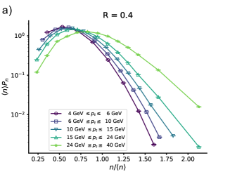
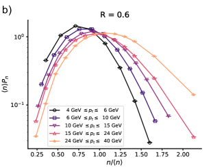
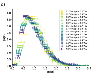
Figure 1: Data from Ref. atlas11 plotted in the KNO form for a) $R=0.4$, b) $R=0.6$. c) Data from Ref. atlas19 .

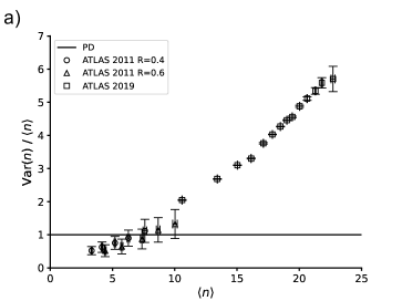
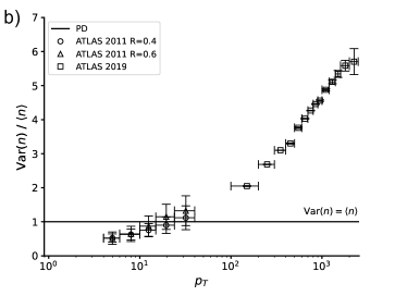
Figure 2: Variance as a function of a) $<n>$ and b) $p_{T}$. Data are from Refs. atlas11 and atlas19 . The solid line shows the result obtained with the Poisson distribution.

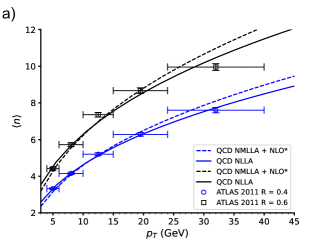
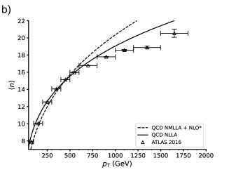
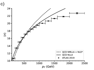
Figure 3: Average multiplicities (data points) obtained from ATLAS, in a) Ref. atlas11 , b) Ref. atlas16 and c) Ref. atlas19 . The curves show the fits with the theoretical expressions Eq. (1) (solid line) and Eq. (2) (dashed line).

In Fig. 1 we plot the ATLAS data on jet multiplicities in the KNO form. In Fig. 1a and Fig. 1b we show the data from Ref. atlas11 on lower $p_{T}$ jets. The two sets refer to two values of the jet $R$ variable. We clearly see that the data violate KNO scaling. However, if we consider the higher $p_{T}$ jets measured in Ref. atlas19 we observe the onset of scaling, as shown in Fig. 1c, specially at $p_{T}>300$ GeV. This change of behavior can be more clearly seen if we plot the ratio between the variance and the average multiplicity ($Var(n)/<n>$) which is equal to one for a Poisson distribution. In Fig. 2 we can see that this ratio is below one for lower $<n>$ (Fig. 2a) and for lower $p_{T}$ (Fig. 2b) and around $<n>\simeq 10$ or $p_{T}\simeq 30$ GeV there is a clear change. The ratio becomes larger than one and we go from sub-poissonian to a super-poissonian distribution. It is tempting to associate this broadening of the multiplicity distribution with transition from quark to gluon initiated jets. In Ref. opal98 the properties of quark and gluon jets were studied. In particular, it was found that the dispersion D of the multiplicity distribution from jets was $D_{g}\simeq 4.37$ and $D_{q}\simeq 4.30$ for gluon and quark jets respectively. The errors quoted in opal98 are very large but these numbers suggest that gluon jets are broader than quark ones and the onset of the dominance of the former could be the dynamical cause of the behavior observed in Fig. 2.

From the low $p_{T}$ data atlas11 we have extracted the average multiplicities for the $R=0.4$ and $R=0.6$ sets. For the higher $p_{T}$ sets the average multiplicities were already given in atlas19 and atlas16 . From the theoretical point of view, the definition of the multiplicity in a jet can be rather tricky. The total hadronic multiplicity within a jet can be obtained from the jet fragmentation function and it was studied in perturbative QCD in several works mu81 ; we84 ; wema ; dre94 ; drega ; re14 . Very recently these calculations have been done with higher precision (see so22 for a recent review of the literature). Here, for simplicity, we shall use the analytical formulas derived from perturbative QCD in the next-to-leading-logarithmic approximation (NLLA) we84 and also, more recently, in the next-to-modified-leading-log approximation (NMLLA) including next-to-leading-order (NLO) corrections to the $\alpha_{s}$ strong coupling re14 . These expressions were successfully applied to fit the multiplicities measured in $e^{+}e^{-}$ collisions delphi98 . The NLLA expression is given by we84 :

$$<n_{ch}>=a\,[\alpha_{s}(p_{T})]^{b}\,e^{c/\sqrt{\alpha_{s}(p_{T})}}\,[1+d\,\sqrt{\alpha_{s}(p_{T})}]$$ (1)

where we84 :

$$b=\frac{1}{4}+\frac{10}{27}\frac{N_{f}}{\beta_{0}}=0.49\hskip 28.45274ptc=\frac{\sqrt{96\pi}}{\beta_{0}}=2.27\hskip 28.45274pt\alpha_{s}(Q^{2})=\frac{4\,\pi}{\beta_{0}\,ln(Q^{2}/\Lambda^{2})}-\frac{\beta_{1}\,ln\,ln(Q^{2}/\Lambda^{2})}{\beta_{0}^{3}\,ln^{2}(Q^{2}/\Lambda^{2})}$$

with $\beta_{0}=11-2/3N_{f}$, $\beta_{1}=102-38/3N_{f}$ and $\Lambda=0.15$ GeV. The NMLLA-NLO expression reads re14 :

$$<n_{ch}>=\mathcal{K}_{ch}\,exp\,\left[2.50217\,\sqrt{Y}-0.491546\,ln\,Y-(0.06889-0.41151\,ln\,Y)\frac{1}{\sqrt{Y}}+(0.00068-0.161658\,ln\,Y)\frac{1}{Y}\right]\\ \\$$ (2)

where

$$Y=ln\,(p_{T}/\Lambda_{QCD})$$

In the above expressions all the parameters have already been fixed so as to reproduce the multiplicity distributions measured in $e^{+}e^{-}$ collisions at LEP and at energies ranging from $2<\sqrt{s}<200$ GeV. In (1) the normalization $a$ and the (higher order corrections) parameter $d$ were adjusted. In (2) the normalization $\mathcal{K}_{ch}$ and $\Lambda_{QCD}$ were adjusted. Both expressions were able to yield very good fits. We assume that each of the two jets in $e^{+}e^{-}$ collisions is initiated by one highly energetic parton, in the same way as the jets observed in $pp$ collisions. Therefore, apart from a normalization factor, the formulas (1) and (2) can be applied to the average multiplicities studied in this work.

In Fig. 3 we show the average multiplicities. As it can be seen, the low $p_{T}$ data from Ref. atlas11 in Fig. 3a are well reproduced both by (1) and (2). The parameters obtained from the fits are shown in Table 1. In comparison to the jets measured in $e^{+}e^{-}$, both the normalization factor and $\Lambda_{QCD}$ are systematically smaller. These expressions work well for the higher $p_{T}$ sets from Ref. atlas16 shown in Fig. 3b and also from Ref. atlas19 shown in Fig. 3c up to $p_{T}\simeq 500-600$ GeV. Up to this point, Eq. (1) and Eq. (2) seem to capture very well the energy dependence of the data. Beyond this point, they overshoot the data. In this region it is possible that gluon recombination (not yet included in the calculations) starts to play a role. In fact $gg\to g$ would reduce the number of produced partons (and hadrons). Qualitatively this effect would go in the right direction to reproduce the data.

	ATLAS 2011 R=0.4	ATLAS 2011 R=0.6	ATLAS 2016	ATLAS 2019	$e^{+}e^{-}$
$\mathcal{K}_{ch}$	0.04(1)	0.06(3)	0.03(2)	0.03(1)	0.117(1)
$\Lambda_{\mathrm{QCD}}$ (GeV)	0.15(8)	0.15(12)	0.15(22)	0.15(19)	0.191(13)
$a$	0.042(5)	0.05(2)	-0.012(9)	-0.015(7)	0.53(6)
$d$	0.9(4)	1.1(1.4)	-13(8)	-11(4)	1.11(39)

Table 1: Fitted values of $\mathcal{K}_{ch}$ and $\Lambda_{\mathrm{QCD}}$ in Eq.(2) and values of $a$ and $d$ in Eq.(1) for all data sets and the corresponding values of these parameters obtained from $e^{+}e^{-}$ collisions in re14 and delphi98 .

III The Sub-Poissonian distribution

A Sub-Poissonian distribution (SPD) is a probability distribution that has a smaller variance than the Poisson one with the same mean. A distribution which has a larger variance is called Super-Poissonian and to this class belongs also the widely used negative binomial distribution (NBD). In shi ; PC-CCS the SPD was introduced in the context of particle physics and applied to study MDs measured at lower energies.

Since the SPD has not been used very often, it is worth saying a few words about its origin and meaning. In particular, we would like to show how it can be obtained from a stochastic Markov process with multiplicity-dependent birth and death rates.

Let $P(n,t)$ be the probability of having $n$ particles at time $t$ and let us consider a very general birth-death process given by the following equations:

$$\!\!\!\!\!\frac{dP(0,t)}{dt} = -\lambda_{0}P(0,t)+\mu_{1}P(1,t),$$ (3)

$$\!\!\!\!\!\frac{dP(n,t)}{dt} = -\left(\lambda_{n}+\mu_{n}\right)P(n,t)+\lambda_{n-1}P(n-1,t)+\mu_{n+1}P(n+1,t),$$ (4)

where $\lambda_{n}$ and $\mu_{n}$ are the birth and death rates when the multiplicity is $n$. Let us further assume that:

$$\lambda_{n}=\lambda{(n+1)^{-\delta}}+\lambda_{0}\quad{\rm and}\quad\mu_{n}=n\mu,$$ (5)

Then, in the steady state, when $\frac{dP(n,t)}{dt}=0$, Eq. (4) yields:

$$-\left[\lambda(n+1)^{-\delta}+\lambda_{0}+n\mu\right]P(n)+(\lambda n^{-\delta}+\lambda_{0})P(n-1)+(n+1)\mu P(n+1)=0$$ (6)

Introducing the notation

$$\frac{\lambda}{\mu}=\alpha\quad{\rm and}\quad\frac{\lambda_{0}}{\mu}=\alpha_{0},$$ (7)

Eq. (6) can be rewritten as :

$$-\left[\alpha(n+1)^{-\delta}+\alpha_{0}+n\right]P(n)+\left[\alpha n^{-\delta}+\alpha_{0}\right]P(n-1)+(n+1)P(n+1)=0$$ (8)

which yields the following recurrence relation

$$(n+1)P(n+1)=\left[\alpha(n+1)^{-\delta}+\alpha_{0}\right]P(n)=g(n)\,P(n)$$ (9)

where $g(n)=(n+1)P(n+1)/P(n)=\alpha(n+1)^{-\delta}+\alpha_{0}$. Knowing $P(0)$, with the above expression we can construct the multiplicity distribution:

$$P(n)=\frac{P(0)}{n!}\prod_{i=0}^{n-1}g(i)=\frac{P(0)}{n!}\prod_{i=0}^{n-1}\left[\alpha(i+1)^{-\delta}+\alpha_{0}\right]$$ (10)

Choosing $\alpha_{0}>0$ and $\delta=-1$ we obtain the Negative Binomial distribution

$$P(n)=\frac{\Gamma(n+k)}{\Gamma(n+1)\Gamma(k)}\alpha^{n}(1-\alpha)^{k}.$$ (11)

where $k=1+\alpha_{0}/\alpha$. In the particular case when $\alpha_{0}=0$, the parameter $k=1$ and the above expression reduces to the geometric (Bose-Einstein) distribution:

$$P(n)=\alpha^{n}(1-\alpha).$$ (12)

Setting $\delta=0$ in (10) we obtain the Poisson distribution :

$$P(n)=\frac{\alpha^{n}}{n!}\exp(-\alpha).$$ (13)

For $\delta>0$ we get the sub-Poissonian distribution:

$$P(n)=c\frac{\alpha^{n}}{(n!)^{1+\delta}},$$ (14)

where $c$ is a normalization factor. Notice that when $\delta=-1$ the above expression becomes (12) apart from a constant factor.

IV From Sub-Poisson to Negative Binomial Distribution

In this section we shall use the form (14) to study the ATLAS data on multiplicity distributions in jets. We will extend the work greg22 and fit all the ATLAS data from Ref. atlas11 and also from Ref. atlas19 . We will fix $\alpha$ and $\delta$ adjusting (14) to the data. The normalization factor $c$ is given in terms of $\alpha$ and $\delta$ as:

$$c=\left(\sum_{1}^{N_{max}}\frac{\alpha^{n}}{(n!)^{1+\delta}}\right)^{-1}$$ (15)

where the $N_{max}$ is the number of data points. The results are shown in Fig. 4a and Fig. 4b. As it can be seen, the SPD can reproduce very well the low $p_{T}$ ATLAS data.

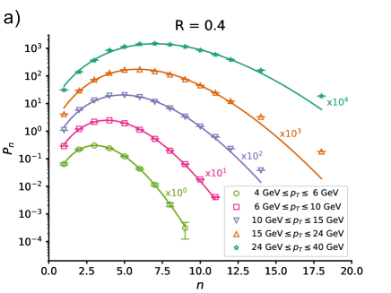
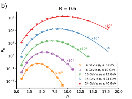
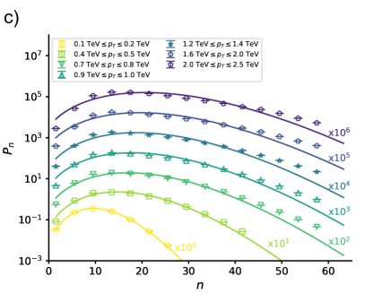
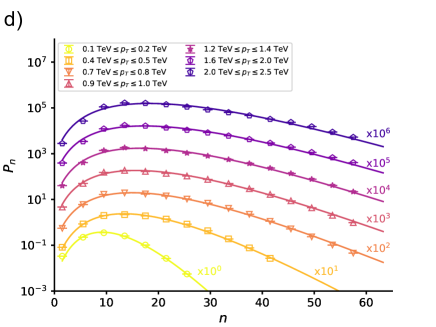
Figure 4: Fits of the ATLAS data on jet multiplicity distributions for a) $R=0.4$ atlas11 , b) $R=0.6$  atlas11 , and data from Ref. atlas19 fitted with a c) Sub-Poisson distribution (14) and d) with a Negative Binomial distribution (16).

The fitted parameters $\alpha$ and $\delta$ are shown in the Tables 3 and 3, as well as the $\chi^{2}$ of the fits, which is always below 2.1. Because of the discrepancies in the large $n$ region, the $\chi^{2}$ of the high $p_{T}$ fits is unreasonably large and we do not show it in Table 5. As seen in Tables 3, 3 and 5, for higher values of $p_{T}$ the $\delta$ parameter becomes negative, which signals the transition from Sub-PD to Super-PD, best visible in Fig. 4c. Notice that the simple formula (14) used here (with the parameter $\delta$ describing the departure from PD towards Sub-PD or Super-PD) approaches the NBD limit (where $\delta=-1$). In Fig. 4d we show lines obtained with the NBD written in a form slightly different from (11) and more convenient for our purposes. From (11) it is easy to see that $\bar{n}=k\,\alpha/(1-\alpha)$ and hence $\alpha^{n}\,(1-\alpha)^{k}=(\bar{n}^{n}\,k^{k})/(\bar{n}+k)^{(n+k)})$. Then (11) can be rewritten as:

$$P(n)=\frac{\Gamma(k+n)}{\Gamma(k)\,\Gamma(n+1)}\frac{\bar{n}^{n}\,k^{k}}{(\bar{n}+k)^{n+k}}.$$ (16)

The fits are very good. They show that $k$ decreases with the jet $p_{T}$ in the same way as it decreases with the energy in NBD fits of the minimum bias multiplicity distributions ge22 . They also show that $\bar{n}/k$ increases with $p_{T}$ indicating the approach to KNO scaling, which is reached when $\bar{n}>>k$. In fact, it was shown in dumi12 that when this ratio reaches $~{}6$ one already has a very good scaling. From the last entries of Table 5 we have ratios close to this number.

$p_{T}$ range (GeV)	$\alpha$	$\delta$	$\chi^{2}$
[4,6]	12.8(2)	1.00(1)	0.06
[6,10]	11.1(4)	0.64(2)	0.32
[10,15]	10.2(5)	0.38(3)	1.36
[15,24]	9.2(6)	0.20(4)	2.08
[24,40]	7.2(5)	-0.02(4)	1.13

Table 2: Fitted $\alpha$ and $\delta$ from Eq. (14) for R=0.4 and data from atlas11 .

$p_{T}$ range (GeV)	$\alpha$	$\delta$	$\chi^{2}$
[4,6]	21.4(9)	0.98(3)	0.30
[6,10]	15.7(3)	0.54(1)	0.06
[10,15]	10.6(4)	0.17(2)	0.46
[15,24]	8.5(6)	0.00(3)	1.55
[24,40]	6.6(6)	-0.18(4)	1.32

Table 3: Fitted $\alpha$ and $\delta$ from Eq. (14) for R=0.6 and data from atlas11 .

$p_{T}$ range (GeV)	$\alpha$	$\delta$
[100,200]	3.13(6)	-0.505(8)
[400,500]	2.30(9)	-0.69(1)
[700,800]	2.0(1)	-0.74(2)
[900,1000]	2.0(1)	-0.76(2)
[1200,1400]	1.9(1)	-0.77(2)
[1600,2000]	1.9(1)	-0.79(2)
[2000,2500]	1.9(2)	-0.79(2)

Table 4: Fitted $\alpha$ and $\delta$ from Eq. (14), for ATLAS 2019 data atlas19 .

$p_{T}$ range (GeV)	$\bar{n}$	$k$
[100,200]	10.5(1)	12(1)
[400,500]	16.0(2)	7.4(4)
[700,800]	18.5(2)	6.0(2)
[900,1000]	19.6(2)	5.7(2)
[1200,1400]	20.8(3)	5.4(3)
[1600,2000]	22.0(4)	5.2(3)
[2000,2500]	23.0(4)	5.2(3)

Table 5: Fitted $\bar{n}$ and $k$ from eq. (16), for ATLAS 2019 data atlas19 .

To summarize, we observe a transition from the low $p_{T}$ region, where there is no KNO scaling, to the high $p_{T}$ region, where we find the scaling shown in Fig. 1c. In our description this is related to the fact that the SPD given by (14) turns into a Super-Poisson distribution for large $p_{T}$ because $\delta$ becomes negative. In turn, the Super-PD distribution transforms for $\delta=-1$ into the geometric distribution (12), i.e. the NBD with $k=1$, for which we have KNO scaling. Therefore, what we observe represents a gradual change in dynamics causing the gradual (with increasing $p_{T}$) emergence of KNO scaling. Multiplicity distributions measured at higher energies are, as shown in vertesi21 ; vertesi22 , better described by NBD. This fact is interesting because it means a transition from one dynamical regime to another shi ; PC-CCS .

A detailed interpretation of these results in terms of the QCD dynamics is beyond the scope of this work but there are hints which may help theorists. The decreasing values of $\alpha$ suggest that the death rate must increase with the energy. In a parton cascade this would mean that the process $gg\to g$ becomes more important and when this happens we are approaching the gluon saturation regime. The initially positive values of $\delta$ render $P(n)$ narrow. This may be a consequence of phase space restrictions. At lower energies we have a smaller number of particles and energy-momentum conservation prevents large fluctuations. At higher energies and larger number of particles the fluctuations are also larger and $P(n)$ becomes broader. Alternatively, the narrowness of $P(n)$ at lower values of $p_{T}$ may indicate that the jets are initiated by quarks. A broader $P(n)$ would indicate the dominance of gluon initiated jets. Further investigation is required.

V Conclusions

In this work we have studied the multiplicity distribution of charged particles within jets in proton-proton collisions, which were measured by the ATLAS collaboration. In the region $p_{T}<500$ GeV the mean multiplicity as a function of the jet transverse momentum is well fitted by the QCD-NLLA and QCD-NMLLA formulas. At higher values of $p_{T}$ these formulas overshoot the data. The low $p_{T}$ data atlas11 do not show KNO scaling, whereas the higher $p_{T}$ data atlas19 gradually approach KNO scaling. This is in line with the PYTHIA simulations presented in Ref. vertesi21 . Using Eq. (14), which, depending on the sign of the $\delta$ parameter describes Sub-Poissonian, Poissonian and Super-Poissonian distributions, we have fitted all the existing data. However, at the highest values of $p_{T}$ the best fit is obtained with the negative binomial distribution. The ratio $\bar{n}/k$ of the NBD fits is large, giving quantitative support to the approach to KNO scaling. The results presented here illustrate the research potential of the analysis of multiplicity distributions in high-energy jets for various values of transverse momenta $p_{T}$. As our analysis shows, different $p_{T}$ ranges are described by different dynamics.

Acknowledgments:

We are grateful to the brazilian funding agencies FAPESP, CNPq and CAPES and also to the INCT-FNA. GW was supported in part by the Polish Ministry of Education and Science, grant Nr 2022/WK/01.

References

- (1) For a review see: W. Kittel, E.A. De Wolf, Soft Multihadron Dynamics, World Scientific, 2005.
- (2) J. F. Grosse-Oetringhaus, K. Reygers, J. Phys. G G37, 083001 (2010).
- (3) Z. Koba, H. B. Nielsen and P. Olesen, Nucl. Phys. B 40, 317 (1972).
- (4) C. S. Lam, M. A. Walton, Phys. Lett. B 140, 246 (1984).
- (5) D. C. Hinz, C. S. Lam, Phys. Rev. D 33 , 3256 (1986).
- (6) S. Hegyi, Nucl. Phys. B (Proc. Suppl.) 92, 122 (2001).
- (7) A. Dumitru and Y. Nara, Phys. Rev. C 85, 034907 (2012).
- (8) A. Dumitru and E. Petreska, arXiv:1209.4105.
- (9) Y. Liu, M. A. Nowak and I. Zahed, Phys. Rev. D 108, 034017 (2023); arXiv:2302.01380 [hep-ph].
- (10) V. Khachatryan et al. [CMS], JHEP 01, 079 (2011).
- (11) G. R. Germano and F. S. Navarra, Phys. Rev. D 105, 014005 (2022); arXiv:2011.08912.
- (12) Y. A. Kulchitsky and P. Tsiareshka, JHEP 10, 111 (2023); Eur. Phys. J. C 82, 462 (2022).
- (13) K. Ackerstaff et al. [OPAL], Eur. Phys. J. C 1, 479 (1998).
- (14) H. W. Ang, M. Rybczyński, G. Wilk, Z. Włodarczyk, Phys. Rev. D 105, 054003 (2022).
- (15) G. Aad et al. (ATLAS Collaboration), Phys. Rev, D 84, 054001 (2011).
- (16) Durham HepData Project: https://www.hepdata.net/record/57743?.
- (17) R. Vértesi, A. Gémes and G. G. Barnaföldi, Phys. Rev. D 103, L051503 (2021).
- (18) Z. Varga and R. Vértesi, Symmetry 14, 1379 (2022).
- (19) G. Aad et al. [ATLAS], Phys. Rev. D 100, 052011 (2019).
- (20) G. Aad et al. [ATLAS], Eur. Phys. J. C 76, 322 (2016).
- (21) A. H. Mueller, Phys. Lett. B 104, 161 (1981).
- (22) B. R. Webber, Phys. Lett. B 143, 501 (1984).
- (23) E. D. Malaza Phys. Lett. B 149, 501 (1984); Phys. B 267, 702 (1986).
- (24) I. M. Dremin and R. C. Hwa, Phys. Lett. B 324, 477 (1994).
- (25) I. M. Dremin and J. W. Gary, Phys. Rept. 349, 301 (2001).
- (26) R. Perez-Ramos and D. d’Enterria, JHEP 08, 068 (2014).
- (27) R. Medves, A. Soto-Ontoso and G. Soyez, JHEP 10, 156 (2022).
- (28) P. Abreu et al. [DELPHI], Phys. Lett. B 416, 233 (1998).
- (29) C. C. Shih, Phys Rev D 34, 2720 (1986).
- (30) P. Carruthers and C. C. Shih, Int. J. Mod. Phys. A 02, 1447 (1987).