Dynamic prediction of death risk given a renewal hospitalization process

Abstract

Predicting the risk of death for chronic patients is highly valuable for informed medical decision-making. This paper proposes a general framework for dynamic prediction of the risk of death of a patient given her hospitalization history, which is generally available to physicians. Predictions are based on a joint model for the death and hospitalization processes, thereby avoiding the potential bias arising from selection of survivors. The framework accommodates various submodels for the hospitalization process. In particular, we study prediction of the risk of death in a renewal model for hospitalizations —a common approach to recurrent event modelling. In the renewal model, the distribution of hospitalizations throughout the follow-up period impacts the risk of death. This result differs from prediction in the Poisson model, previously studied, where only the number of hospitalizations matters. We apply our methodology to a prospective, observational cohort study of 401 patients treated for COPD in one of six outpatient respiratory clinics run by the Respiratory Service of Galdakao University Hospital, with a median follow-up of 4.16 years. We find that more concentrated hospitalizations increase the risk of death.

Keywords: prediction; joint model; frailty; renewal process; hospitalization process; COPD.

1 Introduction

In numerous clinical studies, participants are regularly monitored, and response data, such as biomarkers, vital signs, or hospitalizations, are collected. Additionally, there is often a focus on the time until a specific event occurs, such as death. The longitudinal data collected may be censored by this time-to-event outcome. Therefore, modelling the longitudinal and event-time outcomes separately can lead to biased effect size estimates if the two processes are correlated.¹ Joint modelling of longitudinal and time-to-event data has been a hot topic of research in recent years.²; ³; ⁴ Furthermore, joint models have been proposed for modelling a recurrent event and a terminal event.⁵; ⁶

joint models mitigate the bias in the estimates of covariate effects and allow to quantify and clinically interpret the dependence between both processes. Moreover, joint models provide an outstanding prediction framework, as the paths of both processes —on top of their dependence— is modelled. This paper provides a general dynamic prediction result for the risk of the terminal event given the history of recurrent events. By dynamic we mean that the forecast can be updated throughout the patient’s follow-up, as more data becomes available. The result is general in the sense that it allows for arbitrary recurrent event submodels.

Our development is motivated by the study of the relationship between hospitalizations (the recurrent event) and death for Chronic Obstructive Pulmonary Disease (COPD) patients. Suissa et al. ⁷ studied this relationship using a Cox model for the hazard of death given the number of hospitalizations. joint models for the death and hospitalization processes have also been proposed in other contexts.⁵; ⁸ We believe that this problem is particularly suitable for dynamic prediction as the history of hospitalization is often recorded for chronic patients. Thus, incorporating this information for death risk forecasting may enhance medical decision-making.

We extend the prediction results in Mauguen et al. ⁹, which are valid for a Poisson model for hospitalizations (also known as calendar time model), to a general hospitalization submodel. Our interest lies in considering a gap-time or renewal model for hospitalizations. Indeed, renewal models have usually been considered for the hospitalization process.⁸; ¹⁰; ⁷ We thoroughly study the dependence of the risk of death given the history of hospitalizations for the renewal model. We find that the distribution of hospitalizations during the patient’s follow-up —that is, the timings of the hospitalizations— determines the risk of death. This contrasts with the Poisson model, where only the number of hospitalizations during follow-up matters when predicting the risk of death.⁹ Hence, the renewal model then resembles the clinicians’ decision-making process, where both the number of hospitalizations and the gap-time between hospitalizations are clinically important factors.

This paper is organized as follows. Section 2 introduces the motivating case: the study of risk of death of COPD patients. Section 3 presents the methodological contributions of the paper. In Section 4 we apply our results to predict the risk of death, given the hospitalization history, for COPD patients. Section 5 concludes with a discussion. A technical discussion of the methodological contributions and the results is presented in the Appendices.

2 Motivating study: Risk of death of COPD patients

COPD’s influence on global health and healthcare policies is significant and expanding. It is currently one of the most paradigmatic chronic respiratory condition, with projections indicating further escalation in the years ahead.¹¹ COPD accounted for 3% of all deaths in 2021 across OECD countries,¹² and it was the third leading cause of death in 2019 according to the World Health Organization March 2023 report. The burden of disease will continue to increase, especially in women and regions with low to medium gross domestic product or income. ¹³ The hospitalizations and readmission due to COPD exacerbation significantly impact healthcare utilization. COPD severe exacerbations imply hospital admission, while patients exhibiting a pattern of hospitalizations lead to a deterioration of the patients’ quality of life, which encompasses many dimensions of the patients’ lives.¹⁴

Several prediction models have been developed for COPD readmissions or mortality risk.¹⁵; ¹⁶; ¹⁷; ¹⁸ Furthermore, the increasing hospitalization frequency has been shown to increase the risk of mortality.⁷ Therefore, given the importance of these two outcomes (hospitalization and mortality due to COPD) and their intrinsic relationship, joint modeling of both processes is necessary for two reasons. On the one hand, it reduces the potential bias present in Cox regression models. The bias arises since the fact that long-lived patients tend to experience more hospitalizations could mask the accentuating effect of hospitalizations on the risk of death. On the other hand, it allows to evaluate the effect that hospitalization history (frequency and distribution) has on mortality and to make predictions of mortality risk based on history of hospitalizations during follow-up.

In this work, we considered a prospective, observational cohort study of 401 patients recruited after being treated for COPD in one of six outpatient respiratory clinics run by the Respiratory Service of Galdakao University Hospital. Patients were consecutively included in the study if they had been diagnosed with COPD for at least 6 months and had been stable for at least 6 weeks. The protocol was approved by the Ethics and Research Committees of the hospital (reference 16/14). All candidate patients were given detailed information about the study, and all those included provided written informed consent. Sociodemographic, smoking habits, and clinical variables were recorded. Pulmonary function tests included forced spirometry and body plethysmography, and measurements of carbon monoxide diffusing capacity (DLCO). These tests were performed in accordance with the standards of the European Respiratory Society. ¹⁹ For theoretical values, we considered those of the European Community for Steel and Coal.²⁰ All variables were measured at baseline. The median follow-up time was 4.16 years (interquartile range: 2.58 – 5.16 years). Patient hospitalizations were reviewed during the follow-up period. A brief description of the main variables used for this study is presented in Table 1. More detailed information regarding the dataset can be found elsewhere.²¹

	Number	NA	Median	Interquartile range
Patients	401
Death events	80 (19.9%)
Follow-up time (years)			4.16	2.58 – 5.16
Hospitalization events (total)	425
Hospitalizations per patient			0	0 – 1
Hospitalization length (days)			4	3 – 7
Variables:
Age (years)		0	65	59 – 70
Female	106 (26.4%)	0
DLCO		4	62.5	47.2 – 77.4
$\text{FEV}_{1}$		0	55.8	45 – 68
Previous hosp. $=$ 1	78 (19.4%)	0
Previous hosp. $\geq$ 2	53 (13.2%)	0

Table 1: Descriptive statistics for the whole sample. DLCO = Carbon Monoxide Diffusing Capacity in percentage, $\text{FEV}_{1}$ = forced expiratory volume in one second in percentage, Previous hosp = hospitalizations during the 2 years prior to the start of follow-up.

3 Dynamic prediction of the risk of death given hospitalization history

In this section we obtain the probability of a patient dying between $t$ and $t+w$, given that we observe her hospitalization history up to just before time $t$. The result is based on a joint model for death and hospitalization, which is briefly introduce in Section 3.1. The forecasting expression is given in Section 3.2. This expression is valid for any model for the hospitalization process. We particularize the expression for a renewal model and thoroughly study how the distribution of hospitalizations impacts the forecast of the risk of death (see Section 3.3).

3.1 Joint modeling of death and hospitalization

We briefly introduce the joint model for death, the terminal event, and hospitalization, the recurrent event. A more detailed description can be found in previous work.⁵; ⁶ For each patient $i$ in the sample, we observe the following: (i) the death or censoring time $T_{i}^{d}$, (ii) $\delta_{i}$ an indicator of whether the individual was censored, (iii) $J_{i}$ the number of hospitalizations prior to censoring or death, (iv) $(T_{ij}^{r})_{j=1}^{J_{i}}$ the times for each hospitalization, and (v) $Z_{i}$ a vector of fixed covariates. We consider two (possibly overlapping) collections of the variables in $Z_{i}$, namely $Z_{i}^{d}$ and $Z_{i}^{r}$, that inform about which variables are considered when modelling the death and hospitalization processes, respectively.

The death and hospitalization processes are linked by a individual-specific unobserved frailty variable $u_{i}$. The frailty variable is assumed to be independent of covariates and to have density $g$ supported on $[0,\infty)$. To introduce the model, one must specify $\mathcal{F}_{i}(t)$ — the available information for patient $i$ up to just before time $t$. The information in $\mathcal{F}_{i}(t)$ consists of knowledge about $T_{i}^{d}\geq t$, the frailty variable $u_{i}$, the covariates $Z_{i}$, and the history of hospitalizations up to just before time $t$. To ease notation, we denote the history of hospitalizations prior to $t$ by $H_{i}(t)$. This consists of the number and timing of patient $i$’s hospitalizations before time $t$:

$$H_{i}(t)=\left(J_{i}(t),(T^{r}_{ij})_{j=1}^{J_{i}(t)}\right),\text{ where }J_{i}(t)=\sum_{j=1}^{J_{i}}\mathbf{1}(T_{ij}^{r}<t).$$ (3.1)

The risks for the death process and the hospitalization process, $\alpha^{d}$ and $\alpha^{r}$ respectively, follow a proportional hazards model with frailty:

$$\alpha^{d}(t|\mathcal{F}_{i}(t)) =u_{i}^{\gamma}\cdot\exp\left(\beta_{d}^{\prime}Z^{d}_{i}\right)\cdot\lambda_{0}^{d}(t),\text{ and }$$ (3.2)

$$\alpha^{r}(t|\mathcal{F}_{i}(t)) =u_{i}\cdot\exp\left(\beta_{r}^{\prime}Z_{i}^{r}\right)\cdot\lambda^{r}(t|H_{i}(t)).$$

In the above equations, $\beta_{d}$ and $\beta_{r}$ are the covariates coefficients, $\gamma$ is a parameter that characterizes the relationship between the processes, $\lambda_{0}^{d}$ is the baseline hazard for the death process, and $\lambda^{r}$ is the hazard for the next hospitalization given their history. When $\gamma=0$, the frailty variable does not determine the death risk and the two processes are unrelated. In turn, if $\gamma>0$, hospitalization and death risk are positively related: a higher risk of death correlates with a higher risk of hospitalization. The opposite happens when $\gamma<0$.

The frailty variable $u_{i}$ is generally assumed to follow a gamma distribution with mean one and variance $\theta$. Estimation of the model is based on parametric maximum likelihood, in case one assumes that the baseline hazard functions $\lambda_{0}^{d}$ and $\lambda_{0}^{r}$ are parametric (e.g., Weibull hazards). One could also take a semiparametric approach and approximate the baseline hazards by splines. Estimation is then performed by adding a penalty term to the likelihood that accounts for the complexity of the spline approximation.⁶

It is worth noting that, differently from Mauguen et al. ⁹, we do not require the hospitalization process to be in calendar timescale. The hazard for the next hospitalization may arbitrarily depend on the history of hospitalizations $H_{i}(t)$. The result we present in Section 3.2 for the risk of death given the hospitalization history is valid for a general model for the hospitalization process. In the calendar time or Poisson model (the terminology comes from Cook et al. ²²), we have that $\lambda^{r}(t|H_{i}(t))=\lambda_{0}^{r}(t)$ for a baseline hazard function $\lambda_{0}^{r}$. That is, the hazard for the next hospitalization is independent of the history. In gap timescale or as a renewal model, the hazard of the next hospitalization given their history is

$$\lambda^{r}(t|H_{i}(t))=\lambda_{0}^{r}\left(t-T_{i,J_{i}(t)}^{r}\right),$$ (3.3)

being $\lambda_{0}^{r}$ the baseline hazard function (cf. with eq. (1.5) in Cook et al. ²², where they use counting process notation). As we argue in Section 3.2, the choice of a model for hospitalization greatly impacts the effect of the hospitalization history on the risk of death.

3.2 Dynamic prediction in joint models

We find an expression for the probability of a patient dying between $t$ and $t+w$, given the observed hospitalization history, as implied by the model in (3.2). The expression is valid for any model for the hospitalization process, i.e., for any specification of $\lambda^{r}$. We find that, when hospitalizations follow a renewal model, the forecasted risk of death depends on the distribution of hospitalizations throughout the follow-up period.

Consider that we have followed up a patient during $t$ years. We have thus information regarding her hospitalization history during those years — we know that she was hospitalized exactly in $J$ occasions and that these happened at times $t_{1},\dots,t_{J}$. We refer to this specific realization of the hospitalization history before time $t$ by $h(t)=(J,(t_{j})_{j=1}^{J})$. The probability of interest is

$$\mathbb{P}(t,w|z,h(t))=\operatorname{P}\left(T_{i}^{d}\leq t+w\left|T_{i}^{d}\geq t,Z_{i}=z,H_{i}(t)=h(t)\right.\right),$$ (3.4)

for $t,w\geq 0$.

We first introduce some definitions that are helpful in obtaining the above probability. We define the baseline survival function for death as

$$S_{0}^{d}(t)=\exp\left\{-\int_{0}^{t}\lambda_{0}^{d}(s)ds\right\}.$$ (3.5)

We also introduce the survival function for hospitalizations given their history:

$$S^{r}(t|h(t))=\exp\left\{-\int_{0}^{t}\lambda^{r}(s|h(s))ds\right\}.$$ (3.6)

The above is a survival function in the following sense. If $h^{*}(t)=(0,\emptyset)$ is the hospitalization history that corresponds to no hospitalizations prior to $t$, then $S^{r}(t|h^{*}(t))$ gives the probability of having no hospitalization before time $t$ (see Th. 2.2 in Cook et al. ²²). However, interpretation of $S^{r}(t|h(t))$ is not as straightforward as in the time-to-event case (see Section 3.3). Also, to simplify notation, we denote the proportionality indexes by

$$C_{d}=\exp\left\{\beta_{d}^{\prime}z^{d}\right\}\text{ and }C_{r}=\exp\left\{\beta_{r}^{\prime}z^{r}\right\},$$ (3.7)

where $z^{d}$ and $z^{r}$ are fixed values for the corresponding covariates in the death and hospitalization processes, respectively.

We can now present the main result of this section: the risk of death between $t$ and $t+w$ for a patient with covariate values $Z_{i}=z$ and hospitalization history $H_{i}(t)=h(t)=(J,(t_{j})_{j=1}^{J})$. This risk is given by

$$\mathbb{P}(t,w|z,h(t))=\frac{\int_{0}^{\infty}\left[S_{0}^{d}(t)^{C_{d}u^{\gamma}}-S_{0}^{d}(t+w)^{C_{d}u^{\gamma}}\right]\cdot u^{J}\cdot S^{r}(t|h(t))^{C_{r}u}\cdot g(u)du}{\int_{0}^{\infty}S_{0}^{d}(t)^{C_{d}u^{\gamma}}\cdot u^{J}\cdot S^{r}(t|h(t))^{C_{r}u}\cdot g(u)du}.$$ (3.8)

Note that the above equation is valid for any model $\lambda^{r}$ for the hazard for the next hospitalization given their history. Different models for the hospitalization history will lead to different shapes of $S^{r}$. Below we discuss the Poisson and renewal models.

The derivation of equation (3.8) is based on the independence of the death and hospitalization process given frailty (and covariates) and applications of the Bayes rule. We refer to Appendix A for more details.

Renewal process for hospitalizations

Consider a patient that is hospitalized $J$ times in the follow-up period $[0,t]$. The hospitalization times are $t_{1}<\dots<t_{J}$. In a renewal model the hazard for the next hospitalization at time $s\in[0,t]$ is

$$\lambda^{r}(s|h(s))=\lambda_{0}^{r}\left(s-t_{J(s)}\right),$$ (3.9)

where $\lambda_{0}^{r}$ is a baseline hazard function (e.g., a Weibull hazard) and $J(s)$ is the number of hospitalizations before time $s$. We obtain the shape of the survival function for hospitalizations at the end of the follow-up period: $S^{r}(t|h(t))$. For convenience, let $t_{0}=0$ and $t_{J+1}=t$. We have that

$$\int_{0}^{t}\lambda^{r}(s|h(s))ds=\int_{0}^{t}\lambda_{0}^{r}\left(s-t_{J(s)}\right)ds=\sum_{j=1}^{J+1}\int_{t_{j-1}}^{t_{j}}\lambda_{0}^{r}\left(s-t_{J(s)}\right)ds.$$ (3.10)

Now, for $s\in(t_{j-1},t_{j}]$, the number of hospitalizations prior to $s$ is $J(s)=j-1$. Therefore

$$S^{r}(t|h(t)) =\exp\left\{-\int_{0}^{t}\lambda^{r}(s|h(s))ds\right\}=\prod_{j=1}^{J+1}\exp\left\{-\int_{t_{j-1}}^{t_{j}}\lambda_{0}^{r}\left(s-t_{j-1}\right)ds\right\}$$ (3.11)

$$=\prod_{j=1}^{J+1}\exp\left\{-\int_{0}^{t_{j}-t_{j-1}}\lambda_{0}^{r}\left(s\right)ds\right\}=\prod_{j=1}^{J+1}S^{r}_{0}(t_{j}-t_{j-1}),$$

where $S_{0}^{r}(t)=\exp\{\int_{0}^{t}\lambda_{0}^{r}(s)ds\}$ is the baseline survival function for hospitalizations.

The hazard for the next hospitalization given their history depends on the between hospitalization gap times $t_{j}-t_{j-1}$. Hence, following equation (3.8), the risk of death for two patients, both having $J=2$ hospitalizations, may be different —it will depend on the distribution of the two hospitalizations. In Section 3.3 we discuss which parameters of the model condition the dependence of the risk of death on the distribution of hospitalizations.

Poisson process for hospitalizations

For the sake of comparison, we recover the results in Mauguen et al. ⁹ for the Poisson model for hospitalizations from equation (3.8). In this model, the hazard for the next hospitalization at time $s\in[0,t]$ is $\lambda^{r}(s|h(s))=\lambda_{0}^{r}(s)$, being $\lambda_{0}^{r}$ the baseline hazard for hospitalizations. Then, the survival function for hospitalizations given their history is $S^{r}(t|h(t))=S^{r}_{0}(t)$. This solely depends on the follow-up time and not on the hospitalization times. Plugging in this into equation (3.8) gives equation (5) in Mauguen et al. ⁹, where only the number of hospitalizations ($J$) matters to predict the risk of death.

3.3 Renewal model: relevance of the distribution of hospitalizations

We have argued that, under the renewal model, the distribution of hospitalization plays a significant role in forecasting the risk of death. A natural question to ask then is which pattern of hospitalization times leads to the highest risk of death. Is it when hospitalizations are concentrated or spread out through the follow-up period? In this section we show that the answer depends on the parameters of the model and the shape of the baseline hazard function for hospitalizations. A formal proof of the results is presented in Appendix B.

Recall that in the renewal model the distribution of hospitalizations determines the risk of death through the survival function of hospitalizations given their history:

$$S^{r}(t|h(t))=\prod_{j=1}^{J+1}S^{r}_{0}(t_{j}-t_{j-1}).$$ (3.12)

In this section we fix the follow-up time $t$ and the number of hospitalizations $J$ and study how the risk of death varies with different distributions of $t_{1}<\dots<t_{J}$. We show that two features of the model condition this variation:

1. Whether the death and hospitalization processes are positively or negatively related —the sign of $\gamma$.

2. Whether the baseline hazard for hospitalizations $\lambda_{0}^{r}$ is increasing or decreasing in time.

To study the first point, consider that the two processes are positively related. Since, in this case, $u_{i}^{\gamma}$ is increasing, large values of the frailty variable $u_{i}$ lead a higher risk of death. How does the model update, in a Bayesian fashion, the expected value of the frailty variable for a given distribution of hospitalization times? The relevant term to answer the question is the survival function for hospitalizations: $S^{r}$. We argue that large values of $S^{r}$ imply that the expected value of the frailty variable should be updated upwards.

The key relationship to understand is that of the survival function as the exponential of minus the cumulative hazard: $S^{r}(t|h(t))=\exp\{-\Lambda^{r}(t|h(t))\}$, where $\Lambda^{r}(t|h(t))=-\int_{0}^{t}\lambda^{r}(s|h(s))ds$ (cf. equations (1.3) and (1.5) in Aalen et al. ²³). Intuitively, a large value of the cumulative hazard is associated with low-valued frailty and survival function. On the contrary, a small value for the cumulative hazard is linked to large values for the frailty term and the survival function. The inverse relationship between the cumulative hazard and the survival function is clear from the above equations.

To understand the association between the cumulative hazard and the frailty term, it may help to consider the time-to-event case. If a patient has a large survival time, it accumulates a lot of hazard throughout her extended follow-up period. Also, since the patient has survived for a long time, we may think that she is more resilient (i.e., less fragile) than others. Conversely, a fragile patient will have a short survival period, thus accumulating a smaller amount of hazard.

This relationship between cumulative hazard and frailty also extends to the recurrent event case —that is, to the hospitalization process. We therefore have the following result (c.f. Proposition B.1 in Appendix B).

When the death and hospitalization processes are positively related ($\gamma>0$), larger values of $S^{r}(t|h(t))$ imply a higher risk of death. When the relation is negative ($\gamma<0$), larger values of $S^{r}(t|h(t))$ imply a lower risk of death. If the processes are unrelated ($\gamma=0$), the history of hospitalizations has no effect on the risk of death.

The question now is which distributions of hospitalization times translate into high or low values of $S^{r}$ —equivalently, large values of the cumulative hazard. For the renewal model, we find that this depends on whether the baseline hazard for hospitalizations is increasing or decreasing. To see this, consider two patients which are hospitalized two times during the first year of follow-up. The first patient is hospitalized at months 4 and 8 (dispersed hospitalizations), whereas the second is hospitalized at months 8 and 10 (concentrated). We would like to see which patient accumulates more hazard —i.e., it has a lower-valued survival function.

Figure 1 plots the baseline hazard for hospitalizations and the area below it (the cumulative hazard) for the patient with dispersed (left column) and concentrated (middle column) hospitalizations. We see that, when the hazard is increasing, a patient with a large span of time outside the hospital tends to accumulate more hazard. The opposite happens when the hazard is decreasing. In the right column of the figure, we rearrange the area below the baseline hazards to compare the two. When the hazard is increasing, we see that the cumulative hazard for dispersed hospitalizations fits below the hazard for concentrated hospitalizations (top-right plot in Figure 1). The bottom-right plot, conversely, shows that when the hazard is decreasing the cumulative hazard for concentrated hospitalizations fits below the hazard for dispersed hospitalizations.

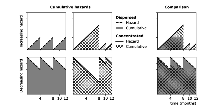
Figure 1: Cumulative hazard for an increasing hazard $\lambda^{r}_{0}(t)=t$ (top row) and a decreasing hazard $\lambda^{r}_{0}(t)=12-t$ (bottom row). In the left column, the hazard $\lambda^{r}(t|h(t))$ for dispersed hospitalizations at times $(t_{1},t_{2})=(4,8)$. In the middle column, the hazard for concentrated hospitalizations at times $(t_{1},t_{2})=(8,12)$. In the right column, we rearrange the area bellow the hazard for dispersed (top row) or concentrated (bottom row) hospitalizations to better compare the two.

We summarize the discussion of this section in a result concerning how the distribution of hospitalizations affects the risk of death in the renewal model (see Theorem B.1 in Appendix B):

The risk of death is highest for dispersed hospitalizations when (i) $\gamma>0$ and the baseline hazard for hospitalizations is increasing or (ii) $\gamma<0$ and the baseline hazard is decreasing.

Conversely, the risk of death is lowest for dispersed hospitalizations when (i) $\gamma>0$ and the baseline hazard is decreasing or (ii) $\gamma<0$ and the baseline hazard is increasing.

We would like to highlight that the above result indicates that the renewal model for hospitalizations is flexible enough to provide a wide range of forecasts for the risk of death. Depending on the parameters of the model —$\gamma$ and the shape of the baseline hazard for hospitalizations—, either concentrated or dispersed hospitalizations will be beneficial regarding the risk of death. Practitioners can compare this with their clinical experience. Thus, the insights from this section equip physicians with a tool to qualitatively assess the model’s fit.

4 Risk of death given hospitalization history for COPD patients

We fit a joint model for hospitalization and death of COPD patients. We consider both a Poisson (calendar timescale) model and a renewal (gap timescale) model for hospitalizations. In the Poisson model, time is measured in “days since inclusion in the study”. In the renewal model, time is measured in “days since inclusion in the study” for the first hospitalization and “days since last hospitalization date” for the following ones. We note that COPD patients tend to have short hospital stays: median of 4 days (see Table 1). Therefore, we keep the timescale as “days”, as opposed to “days out of hospital”.⁸ Prediction results are more interpretable this way.

For both models, we consider Weibull baseline hazards for death and hospitalization. These are given by $\lambda_{0}^{e}(t)=\sigma_{e}t^{\sigma_{e}-1}/b_{e}^{\sigma_{e}}$ for $e=d$ (death) and $e=r$ (hospitalizations). Weibull hazards are specifically suited for the problem: they allow us to rapidly understand how the distribution of hospitalizations will affect the risk of death. Indeed, if the shape parameter satisfies $\sigma_{r}>1$, the baseline hazard for hospitalizations is strictly increasing. If $\sigma_{r}<1$, the baseline hazard is strictly decreasing. We specified a gamma distribution for the frailty variable $u_{i}$, with density $g(u)=u^{1/\theta-1}\exp(-u/\theta)/(\theta^{1/\theta}\Gamma(1/\theta))$. That is, $u_{i}$ has mean one and variance $\theta$.

		Renewal model			Poisson model
		Estimate	SE	P-value	Estimate	SE	P-value
Death	Age (years)	0.121	0.020	0.000	0.122	0.020	0.000
	Female	-0.450	0.399	0.259	-0.434	0.403	0.282
	DLCO	-0.040	0.009	0.000	-0.040	0.009	0.000
	$\text{FEV}_{1}$	-0.025	0.011	0.018	-0.025	0.011	0.018
	Baseline hazard:
	Scale ($b_{d}$)	5355.115	898.040	0.000	5106.744	834.038	0.000
	Shape ($\sigma_{d}$)	1.601	0.165	0.000	1.628	0.168	0.000
Hospitalizations	Age (years)	0.054	0.011	0.000	0.061	0.012	0.000
	Female	0.387	0.220	0.078	0.414	0.237	0.080
	DLCO	-0.016	0.005	0.003	-0.018	0.006	0.002
	$\text{FEV}_{1}$	-0.043	0.007	0.000	-0.047	0.007	0.000
	Prev. hosp $=$ 1	0.479	0.201	0.017	0.537	0.214	0.012
	Prev. hosp $\geq$ 2	0.895	0.219	0.000	1.073	0.234	0.000
	Baseline hazard:
	Scale ($b_{r}$)	3689.577	614.517	0.000	2758.208	348.467	0.000
	Shape ($\sigma_{r}$)	0.845	0.037	0.000	1.148	0.055	0.000
Frailty	$\gamma$	0.760	0.209	0.000	0.734	0.184	0.000
	Variance ($\theta$)	1.127	0.214	0.000	1.451	0.226	0.000

Table 2: Fit results. Sample: 397 patients, 76 death events, and 402 hospitalization events. SE = Standard Error, DLCO = Carbon Monoxide Diffusing Capacity in percentage, $\text{FEV}_{1}$ = Forced expiratory volume in one second in percentage, Prev. hosp = hospitalizations during the 2 years prior to the start of follow-up. Baseline patient: Age = 65, Sex = Male, DLCO = 62.5, FEV = 55.8, Prev. hosp = 0. Log-likelihoods = -3739.286 (renewal) and -3743.491 (Poisson).

Table 2 shows the results obtained for the estimated joint model considering both renewal and Poisson specifications for the hospitalization process. We have included age, sex, DLCO, and forced expiratory volume in 1 second in percentage ($\text{FEV}_{1}$) as common covariates for modelling hospitalization and death processes, and the number of hospitalizations 2 years prior to the first evaluation, for the hospitalization process. This decision was made on the basis of results obtained in previous studies, as well as statistical significance test at 0.05 level. Similar estimates for all the covariates have been obtained in both renewal and Poisson models. In particular in the renewal model, patients with lower values of $\text{FEV}_{1}$ or DLCO have higher risk for hospitalization and dying ($\text{FEV}_{1}$ and DLCO Hazard Ratios (HR) are 0.960 and 0.984 for Hospitalization and 0.975 and 0.961 for Death). Patients face a higher risk as age increases (HR=1.055 and HR=1.129, for Hospitalization and Death, respectively). The results are adjusted by sex, which was not statistically significant. Hospitalization in the two years prior to joining the study were statistically significant for the risk of hospitalization (2 or more HR=2.447). Hospitalization and death risks are positively related ($\gamma=0.760$ and $\gamma=0.734$, in renewal and Poisson models, respectively).

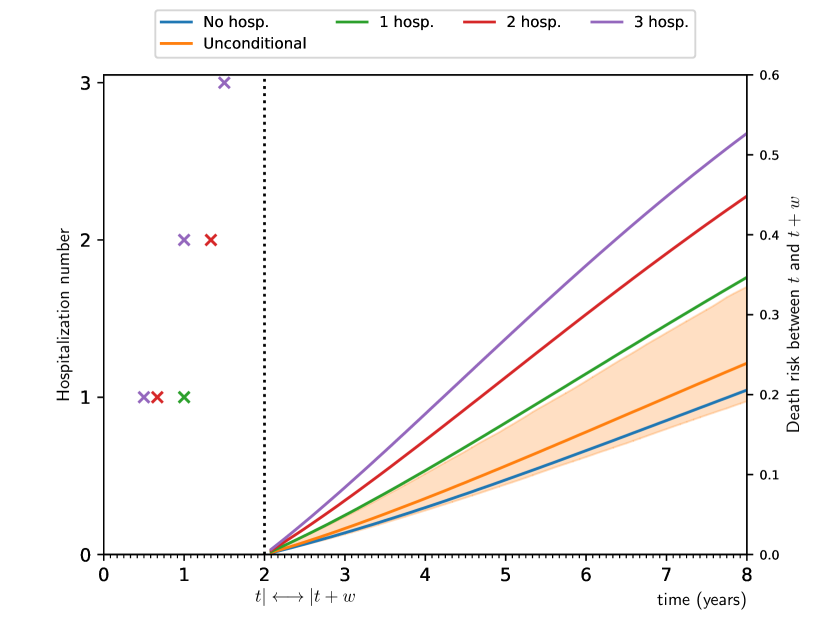
(a) Renewal model. Forecast after 2 years of follow-up.

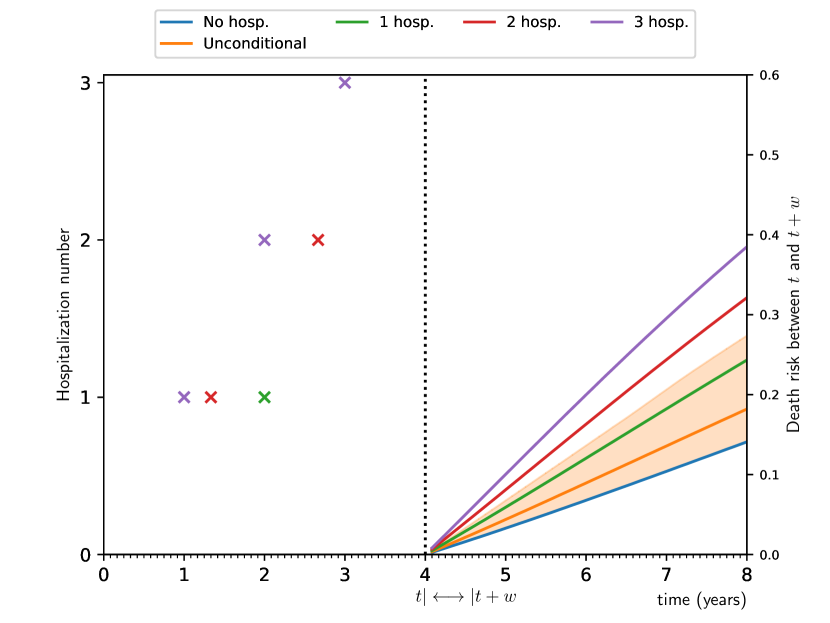
(b) Renewal model. Forecast after 4 years of follow-up.

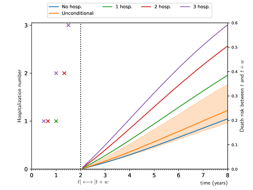
(c) Poisson model. Forecast after 2 years of follow-up.

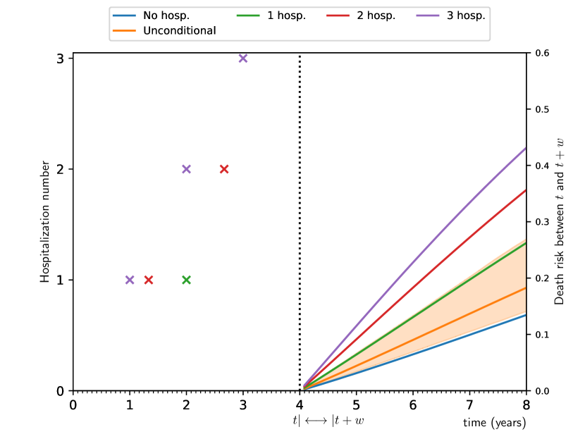
(d) Poisson model. Forecast after 4 years of follow-up.

Figure 2: Prediction of the risk of death given the hospitalization history at different follow-up times. Results for the median patient (65 years-old, male, DLCO of 62.5, $\text{FEV}_{1}$ of 55.8, and with no hospitalizations prior to follow-up) differing on the number of hospitalizations (0 to 3). “Unconditional” means not conditioning on the hospitalization history. Shaded area gives the 90% confidence interval for “Unconditional”.

Figure 2 shows predictions of the risk of death given the history of hospitalizations for four different patients. All of them resemble the median patient (65 years-old, male, DLCO of 62.5, $\text{FEV}_{1}$ of 55.8, and with no hospitalizations prior to follow-up) but experienced a different number of hospitalizations during follow-up: from zero to three. The figure also shows the “Unconditional” risk of death, i.e., not conditioning on the hospitalization history.⁹ Predictions were made at the two and four year marks after follow-up began. Each panel displays the risk of death between $t$ and $t+w$. For instance, the risk of death of the median patient who experiences one hospitalization in the first two years of follow-up, as predicted by the renewal model, is given by the green line in Panel (a). Its value at $5$ is around $0.2$. This means that the risk of death between the second and fifth year, conditional on surviving up to the second, is around 20%.

Several conclusions can be obtained from these results. First, and as it was previously mentioned, conditioning on the number os hospitalizations has an impact on the predicted risk of death, with increasing number of hospitalizations increasing the risk of death. Second, the forecasted risk is smaller under the renewal model than the one under the Poisson model (see for example Panel (a) and Panel (c)). This result is consistent with the interpretation of the renewal hospitalization model as implying the presence of a “perfect physician”, who resets the risk of hospitalization. Indeed, in the renewal model, patients leave the hospital with the same risk as if follow-up had just began. In contrast, the Poisson model implies that physicians take no actions during the recurrent hospitalizations. Third, for predictions shortly after follow-up begins, “Unconditional” is close to “No hospitalizations”. This means that no hospitalizations are generally expected in short follow-up periods. However, for larger follow-up periods (see Panels (b) and (d)), “Unconditional” is closer to “1 hospitalization” which is consistent with the observed data where the mean number of hospitalizations per patient is 1.067.

Table 3 shows the hazard ratios at time $t$ of follow-up. In particular, we can observe the HR for a given number of hospitalizations with respect to not having had any hospitalization up to that time. As can be seen, whatever the follow-up time and for both specifications, increasing the number of hospitalizations during follow-up increases the risk of mortality (for a 2-year follow-up, the HR under de renewal specification are 1.826 and 4.303 for 1 and 5 hospitalizations, respectively). This result contrasts with the result obtained in Suissa et al. ⁷, where an attenuation bias is observed since the HR stabilizes after 3 hospitalizations. In addition, in line with the results shown in Figure 2, HRs are higher for the Poisson model than for the renewal model.

		time in years ($t$)
		1	2	4	6	8
1 hosp.	Renewal	1.837	1.828	1.820	1.820	1.823
	Poisson	2.062	2.072	2.087	2.100	2.112
2 hosp.	Renewal	2.556	2.538	2.520	2.518	2.524
	Poisson	2.934	2.967	3.006	3.036	3.063
3 hosp.	Renewal	3.201	3.178	3.151	3.146	3.155
	Poisson	3.669	3.750	3.835	3.883	3.926
4 hosp.	Renewal	3.782	3.765	3.736	3.728	3.739
	Poisson	4.273	4.427	4.596	4.671	4.730
5 hosp.	Renewal	4.295	4.303	4.285	4.276	4.287
	Poisson	4.753	4.997	5.293	5.415	5.491

Table 3: Hazard Ratios at different follow-up times for patients with different number of hospitalizations. For two hospitalization histories $h(t)$ and $h^{\prime}(t)$, the Hazard Ratio is approximated by $\mathbb{P}(t,w|z,h(t))/\mathbb{P}(t,w|z,h^{\prime}(t))$ for a short window ($w=7$ days). The reference (denominator) has no hospitalizations prior to $t$. Results for the median patient (65 years-old, male, DLCO of 62.5, $\text{FEV}_{1}$ of 55.8, and with no hospitalizations prior to follow-up).

4.1 Dependence on the distribution of hospitalizations

The key result from Section 3.3 is that, in a renewal model for the hospitalization process, the risk of death given hospitalizations depends on the distribution of the later. The dependence is characterized by the relationship between the processes (parameter $\gamma$) and the shape of the baseline hazard for hospitalizations (which, in the Weibull case, corresponds to the parameter $\sigma_{r}$). The estimates of these parameters are (see Table 2)

$$\hat{\gamma}=0.760\text{ and }\hat{\sigma}_{r}=0.845.$$ (4.1)

That is, the death and hospitalization processes are positively related and the baseline hazard for hospitalizations is decreasing in time. According to our results, this means that the risk of death is lowest for dispersed hospitalizations (see Section 3.3).

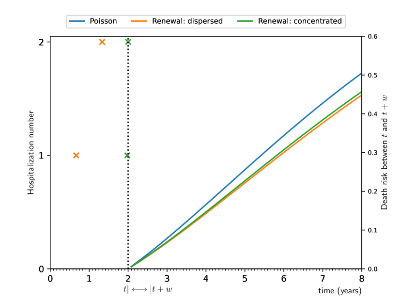
(a) 2 hospitalizations. Forecast after 2 years of follow-up.

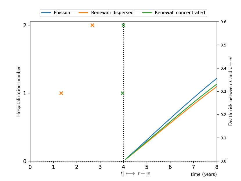
(b) 2 hospitalizations. Forecast after 4 years of follow-up.

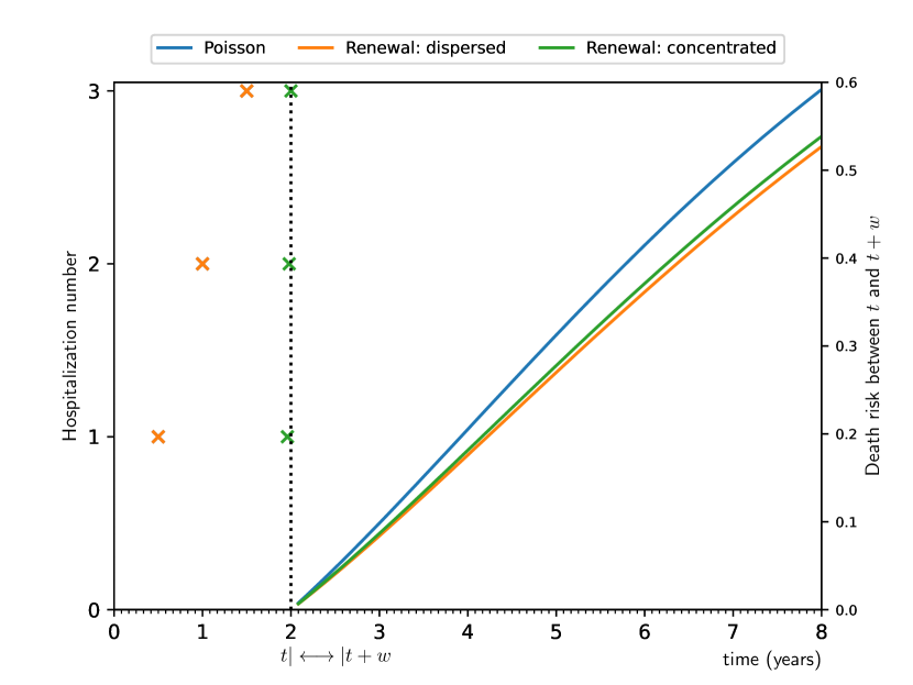
(c) 3 hospitalizations. Forecast after 2 years of follow-up.

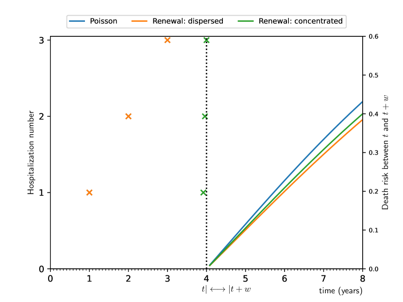
(d) 3 hospitalizations. Forecast after 4 years of follow-up.

Figure 3: Prediction of the risk of death given the hospitalization history at different follow-up times. Results for the median patient (65 years-old, male, DLCO of 62.5, $\text{FEV}_{1}$ of 55.8, and with no hospitalizations prior to follow-up) differing on the timing of the hospitalizations. Letting $t$ denote the follow-up time, dispersed hospitalizations occur at points $(t/3,2t/3)$ and $(t/4,t/2,3t/4)$ for the cases of 2 and 3 hospitalizations, respectively. Concentrated hospitalizations occur at points $(99t/100,t)$ and $(98t/100,99t/100,t)$ for the cases of 2 and 3 hospitalizations, respectively. For the Poisson model, the distribution of hospitalizations is irrelevant (the number matches each case).

Figure 3 shows the prediction of the risk of death given the hospitalization history for four patients with median covariate values. The patients experienced a different number of hospitalizations (2 or 3) during follow-up. Moreover, the distribution of the hospitalizations is dispersed (in orange) or concentrated (in green). As can be observed in all the panels, different predicted risks are estimated (under the renewal model) when hospitalizations occur in a dispersed manner (in orange), or all of them occur in a concentrated pattern (in green), with a higher risk of death for those patients with concentrated hospitalizations.

The differences in terms of risk of death between concentrated and dispersed hospitalizations are sizeable. Table 4 shows the Hazard Ratios at different follow-up times for patients with different distribution of hospitalizations (renewal model) conditioned on all the covariates of the model (i.e. age, sex, DLCO, FEV1). Note that even after conditioning for these clinical and sociodemographic factors, the distribution of the hospitalizations is an important risk factor of death. For instance, at the fourth year, the HR of 3 concentrated hospitalizations versus 3 dispersed hospitalizations (HR=1.052) is equivalent to the HR associated with being 5 months older, holding the remaining clinical characteristics fixed. In addition, for a given number of hospitalizations, the risk of concentrated versus dispersed hospitalizations increases as the follow-up time increases.

	time in years ($t$)
	1	2	4	6	8
2 hosp.	1.017	1.028	1.042	1.051	1.056
3 hosp.	1.021	1.034	1.052	1.063	1.069
4 hosp.	1.022	1.038	1.059	1.072	1.079
5 hosp.	1.021	1.038	1.064	1.079	1.087

Table 4: Hazard Ratios at different follow-up times for patients with different distribution of hospitalizations (renewal model). For two hospitalization histories $h(t)$ and $h^{\prime}(t)$, the Hazard Ratio is approximated by $\mathbb{P}(t,w|z,h(t))/\mathbb{P}(t,w|z,h^{\prime}(t))$ for a short window ($w=7$ days). Fixed the number of hospitalizations, we compute the Hazard Ratio of concentrated hospitalizations over dispersed hospitalizations. Results for the median patient (65 years-old, male, DLCO of 62.5, $\text{FEV}_{1}$ of 55.8, and with no hospitalizations prior to follow-up).

Finally, we propose to statistically test whether the distribution of hospitalization determines the shape of the risk of death. Note that, for a Weibull hazard, the distribution of hospitalizations is irrelevant if either $\gamma=0$ or $\sigma_{r}=1$. That is, the null hypothesis of no relevance of the distribution of hospitalizations is $\operatorname{H}_{0}\colon\gamma=0\text{ or }\sigma_{r}=1$. We construct a Wald test for the equivalent hypothesis $\operatorname{H}_{0}\colon\gamma\cdot(\sigma_{r}-1)=0$ versus $\operatorname{H}_{1}\colon\gamma\cdot(\sigma_{r}-1)\neq 0$. Following Shao ²⁴, p. 433, the test statistic is

$$\hat{W}\equiv\frac{R(\hat{\gamma},\hat{\sigma}_{r})^{2}}{\nabla R(\hat{\gamma},\hat{\sigma}_{r})^{\prime}\hat{V}\nabla R(\hat{\gamma},\hat{\sigma}_{r})},$$ (4.2)

where $R(\gamma,\sigma_{r})=\gamma\cdot(\sigma_{r}-1)$, $\nabla R(\gamma,\sigma_{r})=(\sigma_{r}-1,\gamma)^{\prime}$ is the gradient of $R$, $(\hat{\gamma},\hat{\sigma}_{r})$ is the estimator of the parameters, and $\hat{V}$ is an estimator of the asymptotic covariance matrix of $(\hat{\gamma},\hat{\sigma}_{r})$. Under $\operatorname{H}_{0}$, it holds that $\hat{W}\xrightarrow{P}\chi_{1}^{2}$. We get that, for our fit of the renewal model, $\hat{W}=6.728$ (p-value of $0.009$). Thus, we reject the null hypothesis of no effect of the distribution of hospitalizations on the risk of death.

5 Discussion

We have developed a general dynamic prediction framework for the risk of a terminal event (death) given the recurrent event (hospitalization) history in a joint model setting. The results allow for any intensity-based model for the hospitalization process. Prediction results in this setting, solely for a Poisson process for the recurrent event, where obtained in previous work.⁹ For prediction of a terminal event given the history of a time-dependent marker, see Rizopoulos ² and references therein.

We have studied how the distribution of hospitalizations throughout the follow-up period determines the risk of death when hospitalizations follow-up a renewal process. In contrast to the Poisson case, where solely the number of hospitalization during follow-up matters, we have found that the risk of death depends on the gap times between hospitalizations. The dependence between the risk of death and the distribution of hospitalizations is characterized by two features: whether the two processes are positively or negatively related (parameter $\gamma$) and whether the baseline hazard for hospitalizations is increasing or decreasing.

We have focused in a Weibull model for the baseline hazards. The hazard of this model is monotone, with a single parameter determining whether it is increasing or decreasing. This eases the characterization of the dependence between the risk of death and the distribution of hospitalizations, as it is reduced to two parameters. Nevertheless, our prediction framework allows for other specifications of the baseline hazard. Spline approximations as in Rondeau et al. ⁶ may also be considered when fitting the model. In those cases, if the baseline hazard for hospitalizations is non-monotone, the dependence of the risk of death and the distribution of hospitalizations should be studied for each case —i.e., for each patient and prediction window.

Time-dependent external covariates could be included in the hazard for any of the two processes. Note that time-dependent covariates are usually assumed to be constant in between hospitalizations (see p. 65 in Cook et al. ²²). Under that assumption, one could generalize our results to allow for external time-dependent covariates in the hospitalization process. Regarding time-dependent covariates in the death process, one faces an additional obstacle: the value of the covariates must be known in the time interval $[t,t+w]$. This information is not generally available at the prediction point $t$. So, to forecast with external time-dependent covariates in the death process, the researcher must be willing to assume that the value of these covariates remains unchanged for the whole time interval $[t,t+w]$.

We applied our methodology to a dataset of patients with COPD. We found that the risk of death is higher when the recurrent hospitalization process is modeled using the Poisson specification. The results are in line with the interpretation of the renewal specification as the presence of a “perfect physician” who resets the risk of hospitalization when the patient is discharged. In contrast, in the Poisson specification hospitalizations are independent from each other, that is, as if the physician took no action. Furthermore, in the renewal model, we see that the distribution of hospitalizations is an important risk factor.

There are different avenues for future work. Our results correspond to Setting 1 in Mauguen et al. ⁹ —we believe that our results could be readily extended to cover Setting 2. Moreover, to increase prediction accuracy, it may be of interest to consider the evolution of different biomarkers alongside with the history of hospitalizations. The present paper has solely considered a joint model for the death and hospitalization process. Nevertheless, since biomarker data is often available for chronic patients, it is appealing to include it in the model. This requires proposing a joint model for a terminal, a recurrent, and a longitudinal outcome. How the history of recurrent events and the biomarker jointly determine the risk of the terminal event should also be analyzed.

Additionally, in view of our results, it seems interesting to model hospitalizations as a process that contains a Poisson and a renewal component²⁵ or as a self-exciting process.²⁶ Our prediction result in equation (3.8) is valid for arbitrary models of the hospitalization process. The study of a model with Poisson and renewal components and the characterization of the risk of death given different distributions of hospitalizations is left for future work.

Finally, it is worth mentioning that the software developed to implement the methodological proposal presented in this paper is available on github: https://github.com/telmoperiz/frailtyPredict.

Appendix A Risk of death given the hospitalization history

As in Mauguen et al. ⁹, the derivation in this Appendix is based on the independence of the death and hospitalization process given frailty (and covariates) and applications of the Bayes rule. Additionally, Theorem 2.1 in Cook et al. ²² is used to compute the probability density of a given hospitalization history. This result is valid for arbitrary intensity-based models for the hospitalization process.

The probability of interest is

$$\mathbb{P}(t,w|z,h(t))=\operatorname{P}\left(T_{i}^{d}\leq t+w\left|T_{i}^{d}\geq t,Z_{i}=z,H_{i}(t)=h(t)\right.\right),$$ (A.1)

for $t,w\geq 0$ and hospitalization history $h(t)=(J,(t_{j})_{j=1}^{J})$. As in Mauguen et al. ⁹, conditioning on the frailty variable one gets

$$\mathbb{P}(t,w|z,h(t))=$$ (A.2)

$$\int_{0}^{\infty}\operatorname{P}(T_{i}^{d}\leq t+w|T_{i}^{d}>t,Z_{i}=z,H_{i}(t)=h(t),u_{i}=u)\cdot g(u|T^{d}_{i}>t,Z_{i}=z,H_{i}(t)=h(t))du.$$

We deal with the terms inside the integral separately.

First, using conditional independence of the two processes given frailty and covariates:

$$\operatorname{P}(T_{i}^{d}\leq t+w|T_{i}^{d}>t,Z_{i},H_{i}(t),u_{i}) =\frac{\operatorname{P}(t<T_{i}^{d}\leq t+w|Z_{i},H_{i}(t),u_{i})}{\operatorname{P}(T_{i}^{d}>t|Z_{i},H_{i}(t),u_{i})}$$ (A.3)

$$=\frac{\operatorname{P}(t<T_{i}^{d}\leq t+w|Z_{i},u_{i})}{\operatorname{P}(T_{i}^{d}>t|Z_{i},u_{i})}$$

$$=\frac{\operatorname{P}(T_{i}^{d}>t|Z_{i},u_{i})-\operatorname{P}(T_{i}^{d}>t+w|Z_{i},u_{i})}{\operatorname{P}(T_{i}^{d}>t|Z_{i},u_{i})}.$$

Furthermore, the survival function for death given covariates and the frailty term takes the following shape:

$$\operatorname{P}(T_{i}^{d}>t|Z_{i},u_{i})=\exp\left\{-\int_{0}^{t}\alpha^{d}(s|\mathcal{F}_{i}(s))ds\right\}.$$ (A.4)

This can be obtained by applying Theorem 2.1 in Cook et al. ²² to the “0 death events before $t$” case, noting that (i) “0 death events before $t$” is equivalent to $T_{i}^{d}>t$ and (ii) $\mathcal{F}_{i}(0)=\sigma(Z_{i},u_{i})$. By the model in (3.2), the above equation becomes

$$\operatorname{P}(T_{i}^{d}>t|Z_{i},u_{i}) =\exp\left\{u_{i}^{\gamma}\cdot\exp\left(\beta_{d}^{\prime}Z^{d}_{i}\right)\cdot\left(-\int_{0}^{t}\lambda_{0}^{d}(s)ds\right)\right\}$$ (A.5)

$$=\exp\left\{u_{i}^{\gamma}\cdot\exp\left(\beta_{d}^{\prime}Z^{d}_{i}\right)\cdot\log S_{0}^{d}(t)\right\}$$

$$=\exp\left\{\log\left(S_{0}^{d}(t)^{C_{di}u_{i}^{\gamma}}\right)\right\}=S_{0}^{d}(t)^{C_{di}u_{i}^{\gamma}},$$

where $C_{di}=\exp\left(\beta_{d}^{\prime}Z^{d}_{i}\right)$. Thus, the first part of the integral is

$$\operatorname{P}(T_{i}^{d}\leq t+w|T_{i}^{d}>t,Z_{i},H_{i}(t),u_{i})=\frac{S_{0}^{d}(t)^{C_{di}u_{i}^{\gamma}}-S_{0}^{d}(t+w)^{C_{di}u_{i}^{\gamma}}}{S_{0}^{d}(t)^{C_{di}u_{i}^{\gamma}}}.$$ (A.6)

To compute the second part of the integral, we use Bayes’ rule to write that the conditional density of the frailty variable as

$$g(u|T^{d}_{i}>t,Z_{i}=z,H_{i}(t)=h(t))=$$ (A.7)

$$\frac{\operatorname{P}(T_{i}^{d}>t,H_{i}(t)=h(t)|Z_{i}=z,u_{i}=u)g(u)}{\int_{0}^{\infty}\operatorname{P}(T_{i}^{d}>t,H_{i}(t)=h(t)|Z_{i}=z,u_{i}=u)g(u)du},$$

where we rely on $Z_{i}$ and $u_{i}$ being independent. Moreover, by conditional independence of the two processes given frailty and covariates:

$$\operatorname{P}(T_{i}^{d}>t,H_{i}(t)=h(t)|Z_{i},u_{i})=\operatorname{P}(T_{i}^{d}>t|Z_{i},u_{i})\cdot\operatorname{P}(H_{i}(t)=h(t)|Z_{i},u_{i}).$$ (A.8)

The first term in the product follows from equation (A.5). We apply Theorem 2.1 in Cook et al. ²² to obtain the second term:

$$\operatorname{P}(H_{i}(t)=h(t)|Z_{i},u_{i})=\left(\prod_{j=1}^{J}\alpha^{r}(t_{j}|\mathcal{F}_{i}(t_{j}))\right)\cdot\exp\left\{-\int_{0}^{t}\alpha^{r}(s|\mathcal{F}_{i}(s))ds\right\}.$$ (A.9)

Then, by the model in (3.2),

$$\prod_{j=1}^{J}\alpha^{r}(t_{j}|\mathcal{F}_{i}(t_{j})) =u_{i}^{J}C_{ri}^{J}\prod_{j=1}^{J}\lambda^{r}(t_{j}|H_{i}(t_{j}))\text{ and }$$ (A.10)

$$\exp\left\{-\int_{0}^{t}\alpha^{r}(s|\mathcal{F}_{i}(s))ds\right\} =S^{r}(t|h(t))^{C_{ri}u_{i}},$$

where $C_{ri}=\exp\left(\beta_{r}^{\prime}Z^{r}_{i}\right)$. The result in the second row follows mutatis mutandis from equation (A.5).

We can now plug in the above results into equation (A.7). A key aspect of the model is that, since $C_{ri}^{J}\prod_{j=1}^{J}\lambda^{r}(t_{j}|H_{i}(t_{j}))$ does not depend on $u_{i}$, it cancels out. Thus

$$g(u|T^{d}_{i}>t,Z_{i}=z,H_{i}(t)=h(t))=\frac{S_{0}^{d}(t)^{C_{d}u^{\gamma}}\cdot u^{J}\cdot S^{r}(t|h(t))^{C_{r}u}\cdot g(u)}{\int_{0}^{\infty}S_{0}^{d}(t)^{C_{d}u^{\gamma}}\cdot u^{J}\cdot S^{r}(t|h(t))^{C_{r}u}\cdot g(u)du}.$$ (A.11)

We conclude by putting all the results together to obtain equation (3.8):

$$\mathbb{P}(t,w|z,h(t))=$$ (A.12)

$$\int_{0}^{\infty}\operatorname{P}(T_{i}^{d}\leq t+w|T_{i}^{d}>t,Z_{i}=z,H_{i}(t)=h(t),u_{i}=u)\cdot g(u|T^{d}_{i}>t,Z_{i}=z,H_{i}(t)=h(t))du$$

$$=\frac{\int_{0}^{\infty}\left[S_{0}^{d}(t)^{C_{d}u^{\gamma}}-S_{0}^{d}(t+w)^{C_{d}u^{\gamma}}\right]\cdot u^{J}\cdot S^{r}(t|h(t))^{C_{r}u}\cdot g(u)du}{\int_{0}^{\infty}S_{0}^{d}(t)^{C_{d}u^{\gamma}}\cdot u^{J}\cdot S^{r}(t|h(t))^{C_{r}u}\cdot g(u)du}.$$

Appendix B Distributional effect of hospitalizations in the renewal model

This appendix formally derives the results in Section 3.3. We start by defining the function $\varphi\colon(0,1)\times(0,1)\times(0,1)\to\mathbb{R}$ as

$$\varphi(x,y,z;J,\gamma)\equiv\frac{\int_{0}^{\infty}\left(x^{u^{\gamma}}-y^{u^{\gamma}}\right)\cdot z^{u}\cdot u^{J}\cdot g(u)du}{\int_{0}^{\infty}x^{u^{\gamma}}\cdot z^{u}\cdot u^{J}\cdot g(u)du}.$$ (B.1)

The function depends on the parameters $\gamma$ and $J$. Recall that $\gamma$ measures the degree of dependence between the death and hospitalization process. Then, for a patient with $J$ hospitalizations and and covariates $Z_{i}=z$, the forecasted risk of death is

$$\mathbb{P}(t,w|z,h(t))=\varphi\left(S_{0}^{d}(t)^{C_{d}},S_{0}^{d}(t+w)^{C_{d}},S^{r}(t|h(t))^{C_{r}};J,\gamma\right).$$ (B.2)

The next proposition characterizes the relationship between the risk of death, $\mathbb{P}(t,w|z,h(t))$, and the survival function of hospitalizations given their, history $S^{r}(t|h(t))$.

Proposition B.1

For $\gamma=0$, $\varphi$ is constant in $z$. Moreover, if $x>y$, $\partial\varphi/\partial z$ is positive for $\gamma>0$ and negative for $\gamma<0$.

The proof of the above proposition is provided at the end of the appendix. We note that, if the baseline survival function for death is not constant in $[t,t+w]$, we have that $S_{0}^{d}(t)>S_{0}^{d}(t+w)$. That is, the above proposition can be applied to equation (B.2).

In the renewal model, the survival function of hospitalizations given their history $S^{r}(t|h(t))$ is given by equation (3.12). We study how $S^{r}$ varies with the distribution of hospitalizations. Fix the number of hospitalizations $J\geq 1$ and the follow-up time $t>0$. Hospitalization times are distributed in the following set

$$\mathcal{T}\equiv\{(t_{1},\dots,t_{J})\in\mathbb{R}^{J}\colon 0<t_{1}<\cdots<t_{J}<t\}.$$ (B.3)

The next result characterizes the behavior of $S^{r}$ on this set. Recall that $\lambda_{0}^{r}$ is the baseline hazard for hospitalizations.

Proposition B.2

Suppose that $S^{r}$ is given by equation (3.12). If $\lambda_{0}^{r}$ is strictly increasing:

• $S^{r}$ achieves a maximum value of

  $$\left[S_{0}^{r}\left(\frac{t}{J+1}\right)\right]^{J+1}$$ (B.4)

  on $\mathcal{T}$. The maximum is achieved when $t_{j}=j\cdot t/(J+1)$ for $j\in{1,\dots,J}$.

• For every $(t_{j})_{j=1}^{J}\in\mathcal{T}$, it holds that $S^{r}(t|h(t))\geq S_{0}^{r}(t)$.

On the other hand, if $\lambda_{0}^{r}$ is strictly decreasing:

• $S^{r}$ achieves a minimum value of

  $$\left[S_{0}^{r}\left(\frac{t}{J+1}\right)\right]^{J+1}$$ (B.5)

  on $\mathcal{T}$. The minimum is achieved when $t_{j}=j\cdot t/(J+1)$ for $j\in{1,\dots,J}$.

• For every $(t_{j})_{j=1}^{J}\in\mathcal{T}$, it holds that $S^{r}(t|h(t))\leq S_{0}^{r}(t)$.

To read the proposition, say that $\lambda_{0}^{r}$ is strictly increasing. Then the maximum value of $S^{r}$ is achieved when hospitalizations are equiespaced on $[0,t]$. In this situation, hospitalizations are as dispersed as possible. On the contrary, one of the points where the minimum value of $S^{r}$ is achieved is $t_{j}=t$ for every $j=1,\dots,J$. This point is not feasible since hospitalizations cannot occur simultaneously. What Proposition B.2 says is that, when $\lambda_{0}^{r}$ is strictly increasing, $S^{r}$ tends to its minimum as hospitalizations become more concentrated (i.e., closer to the point $t_{j}=t$ for every $j$). Note that this conclusion holds as long as $S_{0}^{r}$ is continuous, which is generally the case.

The next theorem puts together Propositions B.1 and B.2.

Theorem B.1

In the renewal model, where $S^{r}$ is given by equation (3.12), we have that

• $\mathbb{P}(t,w|z,h(t))$ is highest on $\mathcal{T}$ for $t_{j}=j\cdot t/(J+1)$ (dispersed hospitalizations) when (i) $\gamma>0$ and $\lambda_{0}^{r}$ is increasing or (ii) $\gamma<0$ and $\lambda_{0}^{r}$ is decreasing.

• $\mathbb{P}(t,w|z,h(t))$ is lowest on $\mathcal{T}$ for $t_{j}=j\cdot t/(J+1)$ (dispersed hospitalizations) when (i) $\gamma>0$ and $\lambda_{0}^{r}$ is decreasing or (ii) $\gamma<0$ and $\lambda_{0}^{r}$ is increasing.

Proofs

The proof of Proposition B.1 depends on the following result:

Lemma B.1

For a positive non-degenerate random variable $\xi$ it holds that

• $\operatorname{E}\left[\xi^{1+\gamma}\right]>\operatorname{E}\left[\xi\right]\cdot\operatorname{E}\left[\xi^{\gamma}\right]$ if $\gamma>0$ and

• $\operatorname{E}\left[\xi^{1+\gamma}\right]<\operatorname{E}\left[\xi\right]\cdot\operatorname{E}\left[\xi^{\gamma}\right]$ if $\gamma<0$.

Proof:

Let $f(\gamma)\equiv\operatorname{E}\left[\xi^{1+\gamma}\right]-\operatorname{E}\left[\xi\right]\cdot\operatorname{E}\left[\xi^{\gamma}\right]$. We have that

$$f(\gamma)=\operatorname{E}\left[\xi^{\gamma}\cdot\left(\xi-\operatorname{E}[\xi]\right)\right]=\operatorname{E}\left[\left(\xi^{\gamma}-\operatorname{E}\left[\xi\right]^{\gamma}\right)\cdot\left(\xi-\operatorname{E}[\xi]\right)\right].$$ (B.6)

Consider the function $\phi(x)\equiv x^{\gamma}$ defined for $x>0$. If $\gamma>0$, $\phi$ is strictly increasing. Therefore

$$\xi>\operatorname{E}[\xi]\iff\xi^{\gamma}>\operatorname{E}[\xi]^{\gamma}\text{ almost surely}.$$ (B.7)

Thus, $f$ is the expectation of a non-negative random variable. Since $\xi$ is non-degenerate, the expectation is strictly positive: $f(\gamma)>0$.

If $\gamma<0$, $\phi$ is strictly decreasing and thus $\xi>\operatorname{E}[\xi]\iff\xi^{\gamma}<\operatorname{E}[\xi]^{\gamma}$ almost surely. Then, $f$ is the expectation of a non-positive random variable. Since $\xi$ is non-degenerate, the expectation is strictly negative: $f(\gamma)<0$.

Proof of (Proposition B.1):

First, when $\gamma=0$, $\varphi$ does not depend on $z$:

$$\varphi(x,y,z;J,0)\equiv\frac{\int_{0}^{\infty}\left(x-y\right)\cdot z^{u}\cdot u^{J}\cdot g(u)du}{\int_{0}^{\infty}x\cdot z^{u}\cdot u^{J}\cdot g(u)du}=\frac{x-y}{x}.$$ (B.8)

For $\gamma\neq 0$, taking derivatives of $\varphi$ with respect to $z$:

$$\frac{\partial\varphi}{\partial z}(x,y,z) =\frac{1}{z\cdot\left(\int_{0}^{\infty}u^{J}\cdot x^{u^{\gamma}}\cdot z^{u}\cdot g(u)du\right)^{2}}\left[\int_{0}^{\infty}u^{J+1}\cdot x^{u^{\gamma}}\cdot z^{u}\cdot g(u)du\cdot\int_{0}^{\infty}u^{J}\cdot y^{u^{\gamma}}\cdot z^{u}\cdot g(u)du\right.$$ (B.9)

$$\left.-\int_{0}^{\infty}u^{J+1}\cdot y^{u^{\gamma}}\cdot z^{u}\cdot g(u)du\cdot\int_{0}^{\infty}u^{J}\cdot x^{u^{\gamma}}\cdot z^{u}\cdot g(u)du\right].$$

Define

$$F(x)\equiv\frac{\int_{0}^{\infty}u^{J+1}\cdot x^{u^{\gamma}}\cdot z^{u}\cdot g(u)du}{\int_{0}^{\infty}u^{J}\cdot x^{u^{\gamma}}\cdot z^{u}\cdot g(u)du}.$$ (B.10)

Rearranging terms in the numerator of $\partial\varphi/\partial z$ leads to

$$\frac{\partial\varphi}{\partial z}(x,y,z)>0\iff F(x)>F(y)\text{ and }\frac{\partial\varphi}{\partial z}(x,y,z)<0\iff F(x)<F(y).$$ (B.11)

Since $x>y$, it suffices to check whether $F$ is strictly increasing or decreasing, depending on the sign of $\gamma$. Taking derivatives:

$$\frac{dF}{dx}(x) =\frac{1}{x\cdot\left(\int_{0}^{\infty}u^{J}\cdot x^{u^{\gamma}}\cdot z^{u}\cdot g(u)du\right)^{2}}\left[\int_{0}^{\infty}u^{J+1+\gamma}\cdot x^{u^{\gamma}}\cdot z^{u}\cdot g(u)du\cdot\int_{0}^{\infty}u^{J}\cdot x^{u^{\gamma}}\cdot z^{u}\cdot g(u)du\right.$$ (B.12)

$$\left.-\int_{0}^{\infty}u^{J+1}\cdot x^{u^{\gamma}}\cdot z^{u}\cdot g(u)du\cdot\int_{0}^{\infty}u^{J+\gamma}\cdot x^{u^{\gamma}}\cdot z^{u}\cdot g(u)du\right].$$

Let $m_{\gamma}(u)\equiv u^{J}x^{u^{\gamma}}z^{u}g(u)$. The sign of the derivative of $F$ depends on the sign of the numerator

$$\operatorname{NUM}(\gamma)\equiv\int_{0}^{\infty}u^{1+\gamma}m_{\gamma}(u)du\cdot\int_{0}^{\infty}m_{\gamma}(u)du-\int_{0}^{\infty}um_{\gamma}(u)du\cdot\int_{0}^{\infty}u^{\gamma}m_{\gamma}(u)du$$ (B.13)

Let $M_{\gamma}\equiv\int_{0}^{\infty}m_{\gamma}(u)du>0$ and define the pdf $p_{\gamma}(u)\equiv m_{\gamma}(u)/M_{\gamma}$. We then have that

$$x\cdot\frac{dF}{dx}(x)=\frac{\operatorname{NUM}(\gamma)}{M_{\gamma}^{2}}=\int_{0}^{\infty}u^{1+\gamma}p_{\gamma}(u)du-\int_{0}^{\infty}up_{\gamma}(u)du\cdot\int_{0}^{\infty}u^{\gamma}p_{\gamma}(u)du.$$ (B.14)

We can then apply Lemma B.1 to a random variable $\xi$ with density $p_{\gamma}$ to get the result (recall that $x>0$).

Proof of (Proposition B.2):

Define the baseline cumulative hazard for hospitalizations as $\Lambda_{0}^{r}(t)\equiv\int_{0}^{s}\lambda_{0}^{r}(s)ds$, so that $S_{0}^{r}(t)=\exp\{-\Lambda_{0}^{r}(t)\}$. Also, recall that $t_{0}\equiv 0$ and $t_{J+1}\equiv t$ and let $w_{j}\equiv t_{j}-t_{j-1}$ for $j\in\{1,\dots,J+1\}$. We want to study the behavior of

$$\mathcal{O}(w_{1},\dots,w_{J+1})\equiv\prod_{j=1}^{J+1}S_{0}^{r}(w_{j})$$ (B.15)

as a function of gap times $(w_{1},\dots,w_{J+1})$. The chosen of $w_{j}$’s must satisfy $\sum_{j=1}^{J+1}w_{j}=t_{J+1}-t_{0}=t$ and $w_{j}>0$ for every $j$. Note that

$$-\log\mathcal{O}(w_{1},\dots,w_{J+1})=\sum_{j=1}^{J+1}\Lambda_{0}^{r}(w_{j}).$$ (B.16)

We show the results for strictly increasing $\lambda_{0}^{r}$. The results for strictly decreasing baseline hazard follow mutatis mutandis. If $\lambda_{0}^{r}$ is strictly increasing, then $\Lambda_{0}^{r}$ is a convex function. Therefore, by Jensen’s inequality:

$$\frac{\sum_{j=1}^{J+1}\Lambda_{0}^{r}(w_{j})}{J+1}\geq\Lambda_{0}^{r}\left(\frac{\sum_{j=1}^{J+1}w_{j}}{J+1}\right)=\Lambda_{0}^{r}\left(\frac{t}{J+1}\right)$$ (B.17)

Moreover, equality is achieved if and only if $w_{1}=\cdots=w_{J+1}$. That is, when $w_{j}=t/(J+1)$ for every $j$. The inequality in the above display implies that

$$-\log\mathcal{O}(w_{1},\dots,w_{J+1}) \geq(J+1)\Lambda_{0}^{r}\left(\frac{t}{J+1}\right)\Leftrightarrow$$ (B.18)

$$\mathcal{O}(w_{1},\dots,w_{J+1}) \leq\exp\left\{-(J+1)\Lambda_{0}^{r}\left(\frac{t}{J+1}\right)\right\}.$$

The maximum is achieved when $w_{j}=t/(J+1)$ for every $j$.

To show the condition $\mathcal{O}(w_{1},\dots,w_{J+1})\geq\exp\{-\Lambda_{0}^{r}(t)\}$, let us introduce the sets

$$\mathcal{C}\equiv\left\{w\in\mathbb{R}^{J+1}\colon\sum_{j=1}^{J+1}\Lambda_{0}^{r}(w_{j})\leq\Lambda_{0}^{r}(t)\right\}\text{ and }\mathcal{W}\equiv\left\{w\in\mathbb{R}^{J+1}\colon\sum_{j=1}^{J+1}w_{j}=t,w_{j}\geq 0\right\}.$$ (B.19)

Note that the feasible $w_{j}$’s lie in set $\mathcal{W}$ —precisely, $\mathcal{W}$ is the euclidean closure of the set of feasible $w_{j}$’s. We show that $\mathcal{W}\subseteq\mathcal{C}$. This concludes the proof since it implies that for every feasible $w_{j}$’s

$$\sum_{j=1}^{J+1}\Lambda_{0}^{r}(w_{j})\leq\Lambda_{0}^{r}(t)\Leftrightarrow\mathcal{O}(w_{1},\dots,w_{J+1})\geq\exp\{-\Lambda_{0}^{r}(t)\}.$$ (B.20)

First, since $\Lambda_{0}^{r}$ is convex, for $w,w^{\prime}\in\mathcal{C}$ and $\eta\in[0,1]$:

$$\sum_{j=1}^{J+1}\Lambda_{0}^{r}(\eta w_{j}+(1-\eta)w_{j}^{\prime})\leq\eta\sum_{j=1}^{J+1}\Lambda_{0}^{r}(w_{j})+(1-\eta)\sum_{j=1}^{J+1}\Lambda_{0}^{r}(w_{j}^{\prime})\leq\Lambda_{0}^{r}(t),$$ (B.21)

so $\mathcal{C}$ is a convex set. Then, define $\tau^{j}\in\mathbb{R}^{J+1}$ as the vector which takes value $t$ at coordinate $j$ and 0 everywhere else: $\tau_{i}^{j}=t\iff i=j$ and $\tau_{i}^{j}=0\iff i\neq j$. Note that $\tau^{j}\in\mathcal{C}$ for every $j$. Moreover, for every $w\in\mathcal{W}$, $w=\sum_{j=1}^{J+1}\eta_{j}\tau^{j}$ with $\eta_{j}\equiv w_{j}/t$. Since $\eta_{j}\geq 0$ for every $j$ and $\sum_{j=1}^{J+1}\eta_{j}=1$, this means that every $w\in\mathcal{W}$ may be written as a convex combination of $\tau^{j}$’s. Thus, $\tau^{j}$ being in $\mathcal{C}$ and $\mathcal{C}$ being convex implies $\mathcal{W}\subseteq\mathcal{C}$.

Proof of (Theorem B.1):

Suppose that $\gamma>0$. By Proposition B.1 and $C_{r}>0$,

$$z\mapsto\varphi\left(S_{0}^{d}(t)^{C_{d}},S_{0}^{d}(t+w)^{C_{d}},z^{C_{r}};J,\gamma\right)$$ (B.22)

is a strictly increasing transformation. Thus, the maximizer and minimizer of $\mathbb{P}(t,w|z,h(t))$ on $\mathcal{T}$ coincide with the maximizer and minimizer of $S^{r}(t|h(t))$ on $\mathcal{T}$. By Proposition B.2, $t_{j}=j\cdot t/(J+1)$ is a maximizer when $\lambda_{0}^{r}$ is increasing and a minimizer when $\lambda_{0}^{r}$ is decreasing.

If $\gamma<0$, Proposition B.1 states that

$$z\mapsto\varphi\left(S_{0}^{d}(t)^{C_{d}},S_{0}^{d}(t+w)^{C_{d}},z^{C_{r}};J,\gamma\right)$$ (B.23)

is a strictly decreasing transformation. This means that a maximizer of $S^{r}(t|h(t))$ on $\mathcal{T}$ is a minimizer of $\mathbb{P}(t,w|z,h(t))$ on $\mathcal{T}$. Also, a minimizer of $S^{r}(t|h(t))$ on $\mathcal{T}$ is a maximizer of $\mathbb{P}(t,w|z,h(t))$ on $\mathcal{T}$. The conclusion for this case follows by applying Proposition B.2 again.

References

- Ibrahim et al. 2010 Ibrahim JG, Chu H, and Chen LM. Basic concepts and methods for joint models of longitudinal and survival data. Journal of clinical oncology, 28(16):2796, 2010.
- Rizopoulos 2012 Rizopoulos D. Joint models for longitudinal and time-to-event data: With applications in R. CRC press, 2012.
- Asar et al. 2015 Asar Ö, Ritchie J, Kalra PA, and Diggle PJ. Joint modelling of repeated measurement and time-to-event data: an introductory tutorial. International journal of epidemiology, 44(1):334–344, 2015.
- Hickey et al. 2016 Hickey GL, Philipson P, Jorgensen A, and Kolamunnage-Dona R. Joint modelling of time-to-event and multivariate longitudinal outcomes: recent developments and issues. BMC medical research methodology, 16:1–15, 2016.
- Liu et al. 2004 Liu L, Wolfe RA, and Huang X. Shared frailty models for recurrent events and a terminal event. Biometrics, 60(3):747–756, 2004.
- Rondeau et al. 2007 Rondeau V, Mathoulin-Pelissier S, Jacqmin-Gadda H, Brouste V, and Soubeyran P. Joint frailty models for recurring events and death using maximum penalized likelihood estimation: application on cancer events. Biostatistics, 8(4):708–721, 2007.
- Suissa et al. 2012 Suissa S, Dell’Aniello S, and Ernst P. Long-term natural history of chronic obstructive pulmonary disease: severe exacerbations and mortality. Thorax, 67(11):957–963, 2012.
- González et al. 2005 González JR, Fernandez E, Moreno V, Ribes J, Peris M, Navarro M, Cambray M, and Borràs JM. Sex differences in hospital readmission among colorectal cancer patients. Journal of Epidemiology & Community Health, 59(6):506–511, 2005.
- Mauguen et al. 2013 Mauguen A, Rachet B, Mathoulin-Pélissier S, MacGrogan G, Laurent A, and Rondeau V. Dynamic prediction of risk of death using history of cancer recurrences in joint frailty models. Statistics in medicine, 32(30):5366–5380, 2013.
- Louzada et al. 2017 Louzada F, Macera MA, and Cancho VG. A gap time model based on a multiplicative marginal rate function that accounts for zero-recurrence units. Statistical Methods in Medical Research, 26(5):2000–2010, 2017.
- Soriano et al. 2020 Soriano JB, Kendrick PJ, Paulson KR, Gupta V, Abrams EM, Adedoyin RA, Adhikari TB, Advani SM, Agrawal A, Ahmadian E, and others . Prevalence and attributable health burden of chronic respiratory diseases, 1990–2017: a systematic analysis for the global burden of disease study 2017. The Lancet Respiratory Medicine, 8(6):585–596, 2020.
- OECD 2023 OECD . Health at a Glance 2023: OECD Indicators. OECD Publishing, 2023.
- Boers et al. 2023 Boers E, Barrett M, Su JG, Benjafield AV, Sinha S, Kaye L, Zar HJ, Vuong V, Tellez D, Gondalia R, and others . Global burden of chronic obstructive pulmonary disease through 2050. JAMA Network Open, 6(12):e2346598–e2346598, 2023.
- Esteban et al. 2020 Esteban C, Arostegui I, Aramburu A, Moraza J, Najera-Zuloaga J, Aburto M, Aizpiri S, Chasco L, and Quintana JM. Predictive factors over time of health-related quality of life in copd patients. Respiratory Research, 21:1–11, 2020.
- Quintana et al. 2022 Quintana JM, Anton-Ladislao A, Orive M, Aramburu A, Iriberri M, Sánchez R, Jiménez-Puente A, Miguel-Díez dJ, Esteban C, and group RR. Predictors of short-term copd readmission. Internal and emergency medicine, 17(5):1481–1490, 2022.
- Shah et al. 2022 Shah SA, Nwaru BI, Sheikh A, Simpson CR, and Kotz D. Development and validation of a multivariable mortality risk prediction model for copd in primary care. NPJ Primary Care Respiratory Medicine, 32(1):21, 2022.
- Aramburu et al. 2019 Aramburu A, Arostegui I, Moraza J, Barrio I, Aburto M, García-Loizaga A, Uranga A, Zabala T, Quintana JM, and Esteban C. Copd classification models and mortality prediction capacity. International journal of chronic obstructive pulmonary disease, pages 605–613, 2019.
- Arostegui et al. 2019 Arostegui I, Legarreta MJ, Barrio I, Esteban C, Garcia-Gutierrez S, Aguirre U, Quintana JM, Group IC, and others . A computer application to predict adverse events in the short-term evolution of patients with exacerbation of chronic obstructive pulmonary disease. JMIR Medical Informatics, 7(2):e10773, 2019.
- Ph 1993 Ph Q. Lung volumes and forced expiratory flows. report working party standardization of lung function tests. european community for steel and coal. official statement of the european respiratory society. Eur. Respir. J., 16:5–40, 1993.
- Stanojevic et al. 2020 Stanojevic S, Graham BL, Cooper BG, Thompson BR, Carter KW, Francis RW, and Hall GL. Official ers technical standards: Global lung function initiative reference values for the carbon monoxide transfer factor for caucasians. European Respiratory Journal, 56(1750010), 2020.
- Esteban et al. 2024 Esteban C, Aguirre N, Aramburu A, Moraza J, Chasco L, Aburto M, Aizpiri S, Golpe R, and Quintana JM. Influence of physical activity on the prognosis of copd patients: the hado. 2 score–health, activity, dyspnoea and obstruction. ERJ Open Research, 10(1), 2024.
- Cook et al. 2007 Cook RJ, Lawless JF, and others . The statistical analysis of recurrent events. Springer, 2007.
- Aalen et al. 2008 Aalen O, Borgan O, and Gjessing H. Survival and event history analysis: a process point of view. Springer Science & Business Media, 2008.
- Shao 2003 Shao J. Mathematical statistics. Springer Science & Business Media, 2003.
- Ng and Cook 1997 Ng ET and Cook RJ. Modeling two-state disease processes with random effects. Lifetime Data Analysis, 3:315–335, 1997.
- Kopperschmidt and Stute 2013 Kopperschmidt K and Stute W. The statistical analysis of self-exciting point processes. Statistica Sinica, pages 1273–1298, 2013.