Variational Flow Matching for Graph Generation

Abstract

We present a formulation of flow matching as variational inference, which we refer to as variational flow matching (VFM). Based on this formulation we develop CatFlow, a flow matching method for categorical data. CatFlow is easy to implement, computationally efficient, and achieves strong results on graph generation tasks. In VFM, the objective is to approximate the posterior probability path, which is a distribution over possible end points of a trajectory. We show that VFM admits both the CatFlow objective and the original flow matching objective as special cases. We also relate VFM to score-based models, in which the dynamics are stochastic rather than deterministic, and derive a bound on the model likelihood based on a reweighted VFM objective. We evaluate CatFlow on one abstract graph generation task and two molecular generation tasks. In all cases, CatFlow exceeds or matches performance of the current state-of-the-art models.

1 Introduction

In recent years, the field of generative modeling has seen notable advancements. In image generation [35, 38], the development and refinement of diffusion-based approaches — specifically those using denoising score matching [51] — have proven effective for generation at scale [14, 46]. However, while training can be done effectively, the constrained space of sampling probability paths in a diffusion requires tailored techniques to work [44, 56]. This is in contrast to more flexible approaches such as continuous normalizing flows (CNFs) [8], that are able to learn a more general set of probability paths than diffusion models [45], at the expense of being expensive to train as they require one to solve an ODE during each training step (see e.g. [5, 39, 13]).

Recently, Lipman and collaborators [24] proposed flow matching (FM), an efficient and simulation-free approach to training CNFs. Concretely, they use a per-sample interpolation to derive a simpler objective for learning the marginal vector field that generates a desired probability path in a CNF. This formulation provides equivalent gradients without explicit knowledge of the (generally intractable) marginal vector field. This work has been extended to different geometries [7, 20] and various applications [52, 9, 12, 21]. Similar work has been proposed concurrently in [27, 1].

This paper identifies a reformulation of flow matching that we refer to as variational flow matching (VFM). In flow matching, the vector field at any point can be understood as the expected continuation toward the data distribution. In VFM, we explicitly parameterize the learned vector field as an expectation relative to a variational distribution. The objective of VFM is then to minimize the Kullback-Leibler (KL) divergence between the posterior probability path, i.e. the distribution over possible end points (continuations) at a particular point in the space, and the variational approximation.

We show that VFM recovers the original flow matching objective when the variational approximation is Gaussian and the conditional vector field is linear in the data. Under the assumption of linearity, a solution to the VFM problem is also exact whenever the variational approximation matches the marginals of the posterior probability path, which means that we can employ a fully-factorized variational approximation without loss of generality.

While VFM provides a general formulation, our primary interest in this paper is its application to graph generation, where the data are categorical. This setting leads to a simple method that we refer to as CatFlow, in which the objective reduces to training a classifier over end points on a per-component basis. We apply CatFlow to a set of graph generation tasks, both for abstract graphs [30] and molecular generation [34, 18]. By all metrics, our results match or substantially exceed those obtained by existing methods.

2 Background

2.1 Transport Framework for Generative Modeling and CNFs

Common generative modeling approaches such as normalizing flows [36, 32] and diffusion models [14, 46] parameterize a transformation $\varphi$ from some initial tractable probability density $p_{0}$ – typically a standard Gaussian distribution – to the target data density $p_{1}$. In general, there is a trade-off between allowing $\varphi$ to be expressive enough to model the complex transformation while ensuring that the determinant term is still tractable. One such transformation is a continuous normalizing flow (CNF).

Any time-dependent vector field $v_{t}:[0,1]\times\mathbb{R}^{D}\to\mathbb{R}^{D}$ gives rise to such a transformation – called a flow – as such a field induces a time-dependent diffeomorphism $\varphi_{t}:[0,1]\times\mathbb{R}^{D}\to\mathbb{R}^{D}$ defined by the following ordinary differential equation (ODE):

$$\frac{d}{dt}\varphi_{t}(x) =v_{t}(\varphi_{t}(x))\text{ with initial conditions }\varphi_{0}(x)=x.$$ (1)

In CNFs, this vector field is learned using a neural network $v_{t}^{\theta}$. Through the change of variables formula $p_{t}(x)$ can be evaluated (see appendix D) and hence one could try and optimize the empirical divergence between the resulting distribution $p_{1}$ and target distribution. However, obtaining a gradient sample for the loss requires ones to solve the ODE induced during training, making this approach computationally expensive.

2.2 Flow Matching

In flow matching [24], the aim is to regress the underlying vector field of a CNF directly on the interval $t\in[0,1]$. Flow matching leverages the fact that even though we do not have access to the actual underlying vector field – which we denote as $u_{t}$ – and probability path $p_{t}$, one can construct a per-example formulation by defining conditional flows, i.e. the trajectories towards specific datapoints $x_{1}$. Concretely, FM sets:

$$u_{t}(x)=\int u_{t}(x\mid x_{1})\frac{p_{t}(x\mid x_{1})p_{\text{data}}(x_{1})}{p_{t}(x)}\mathrm{d}x_{1},$$ (2)

where $u_{t}(x\mid x_{1})$ is the conditional trajectory. The most common way to define $u_{t}(x\mid x_{1})$ is as the straight line continuation from $x$ to $x_{1}$, implying one can obtain samples $x\sim p_{t}(x\mid x_{1})$ simply by interpolating samples $x_{0}\sim p_{0}$ for some $p_{0}$ and $x_{1}\sim p_{1}$,

$$u_{t}(x\mid x_{1}):=\frac{x_{1}-x}{1-t}\implies x=tx_{1}+(1-t)x_{0}\text{ is a sample }x\sim p_{t}(x\mid x_{1}).$$ (3)

Crucially, the flow matching objective

$$\mathcal{L}_{\text{FM}}(\theta)=\mathbb{E}_{t\sim[0,1],x\sim p_{t}(x)}\left[\big{\|}v_{t}^{\theta}(x)-u_{t}(x)\big{\|}_{2}^{2}\right]$$ (4)

is equivalent in expectation (up to a constant) to the conditional flow matching objective

$$\mathcal{L}_{\text{CFM}}(\theta)=\mathbb{E}_{t\sim[0,1],x_{1}\sim p_{\text{data}}(x_{1}),x\sim p_{t}(x\mid x_{1})}\left[\big{\|}v_{t}^{\theta}(x)-u_{t}(x\mid x_{1})\big{\|}_{2}^{2}\right].$$ (5)

An advantage of flow matching is that this conditional trajectory $u_{t}(x\mid x_{1})$ can be chosen to make the problem tractable. The authors show that diffusion models can be instantiated as flow matching with a specific conditional trajectory, but also show that assuming a simple, straight-line trajectory leads to more efficient training. Note that in contrast to likelihood-based training of CNFs, flow matching is simulation free, leading to a scalable approach to learning CNFs.

3 Variational Flow Matching for Graph Generation

We derive CatFlow through a novel, variational view on flow matching we call Variational Flow Matching (VFM). The VFM framework relies on two insights. First, we can define the marginal vector field and its approximation in terms of an expectation with respect to a distribution over end points of the transformation. This implies that we can map a flow matching problem onto a variational counterpart, opening up the usage of variational inference techniques. Second, under typical assumptions on the forward process, we can decompose the expected conditional vector field into components for individual variables which can be computed in terms of the marginals of the distribution over end points of the conditional trajectories. This implies that, without loss of generality, we can solve a VFM problem using a fully-factorized variational approximation, providing a tractable approximate vector field. For categorical data, the corresponding vector field can be computed efficiently via direct summation. This results in a closed-form objective to train CNFs for categorical data, which we refer to as CatFlow. Note that we develop the theory of VFM in section 3 and we relate VFM to flow matching and score-based diffusion in section 4.

3.1 Flow Matching using Variational Inference

In any flow matching problem, the vector field in eq. 2 can be expressed as an expectation

$$u_{t}(x) =\int u_{t}(x\mid x_{1})p_{t}(x_{1}\mid x)\mathrm{d}x_{1}=\mathbb{E}_{p_{t}(x_{1}\mid x)}\left[u_{t}(x\mid x_{1})\right],$$ (6)

where $p_{t}(x_{1}\mid x)$ is the posterior probability path, the distribution over possible end points $x_{1}$ of paths passing through $x$ at time $t$,

$$p_{t}(x_{1}\mid x) :=\frac{p_{t}(x,x_{1})}{p_{t}(x)}, p_{t}(x,x_{1}) :=p_{t}(x\mid x_{1})\>p_{\text{data}}(x_{1}).$$ (7)

This makes intuitive sense: the velocity in point $x$ is given by all the continuations from $x$ to final points $x_{1}$, weighted by how likely that final point is given that we are at $x$. Note that to compute $u_{t}(x)$, one has to evaluate a joint integral over $D$ dimensions.

This observation leads us to propose a change in perspective. Rather than predicting the vector field directly, we can define an approximate vector field in terms of an expectation with respect to a variational distribution $q_{t}^{\theta}$ with parameters $\theta$,

$$v_{t}^{\theta}(x):=\int u_{t}(x\mid x_{1})q_{t}^{\theta}(x_{1}\mid x)\mathrm{d}x_{1}.$$ (8)

Clearly, in this construction $v_{t}^{\theta}(x)$ will be equal to $u_{t}(x)$ when $q_{t}^{\theta}(x_{1}\mid x)$ and $p_{t}(x_{1}\mid x)$ are identical. This implies that we can map a flow matching problem onto a variational inference problem.

Concretely, we can define a variational flow matching problem by minimizing the Kullback-Leibler (KL) divergence from $p_{t}$ to $q_{t}^{\theta}$, which we can express as (see section A.1 for derivations)

$$\mathbb{E}_{t}\left[\text{KL}\big{(}p_{t}(x)p_{t}(x_{1}\mid x)~{}||~{}p_{t}(x)q^{\theta}_{t}(x_{1}\mid x)\big{)}\right]=-\mathbb{E}_{t,x,x_{1}}\left[\log q_{t}^{\theta}(x_{1}\mid x)\right]+\text{const},$$ (9)

where $t\sim\text{Uniform}(0,1)$ and $x,x_{1}\sim p_{t}(x,x_{1})$.

This leads us to propose the variational flow matching (VFM) objective

$$\mathcal{L}_{\text{VFM}}(\theta)=-\mathbb{E}_{t,x,x_{1}}\left[\log q_{t}^{\theta}(x_{1}\mid x)\right].$$ (10)

Note that, though different, this objective is similar to a typical negative log-likelihood objective.

At this stage of the exposition, it is not yet clear how useful this variational perspective on flow matching is in practice. First, while we can in principle map any flow matching problem onto a variational inference problem, this requires learning an approximation of a potentially complex, high-dimensional distribution $p_{t}(x_{1}\mid x)$. Second, we express $v^{\theta}_{t}(x)$ as an expectation, which could well be intractable. This could mean that we would have to approximate this expectation, for example using a Monte Carlo estimator. We will address these concerns in section 3.2.

3.2 Mean-Field Variational Flow Matching

Decomposing the conditional vector field.

At first glance we do not seem to obtain much from this variation view due to the intractability of $p_{t}(x_{1}\mid x)$ and $v_{t}^{\theta}(x)$. Fortunately, we can simplify the objective and the calculation of the marginal vector field under certain conditions on the conditional vector field. Specifically, we will focus on the special case where the conditional vector field $u_{t}(x\mid x_{1})$ is linear in $x_{1}$, such as in straight line interpolations commonly used in flow matching. Informally, we show that in that case the specific form of the distribution used does not affect the expected value of the conditional vector field as long as the marginals coincide. As such, the solution can be found by a mean-field/factorized distribution exactly. This reduces the problem from one high-dimensional problem, into a series of low dimension problems. Formally, the following holds:

Theorem 1.

Assume that the conditional vector field $u_{t}(x\mid x_{1})$ is linear in $x_{1}$. Then, for any distribution $r_{t}(x_{1}\mid x)$ such that the marginal distributions coincide with those of $p_{t}(x_{1}\mid x)$, the corresponding expectations of $u_{t}(x\mid x_{1})$ are equal, i.e.

$$\mathbb{E}_{r_{t}(x_{1}\mid x)}\left[u_{t}(x\mid x_{1})\right]=\mathbb{E}_{p_{t}(x_{1}\mid x)}\left[u_{t}(x\mid x_{1})\right].$$ (11)

We provide a proof in section A.3. It follows directly from theorem 1 that without loss of generality we can consider the considerably easier task of a fully-factorized approximation

$$q_{t}^{\theta}(x_{1}\mid x):=\prod_{d=1}^{D}q_{t}^{\theta}(x_{1}^{d}\mid x).$$ (12)

We refer to this special case as mean-field variational flow matching (MF-VFM), and the VFM objective reduces to

$$\mathcal{L}_{\text{MF-VFM}}(\theta)=-\mathbb{E}_{t,x,x_{1}}\left[\log q_{t}^{\theta}(x_{1}\mid x)\right]=-\mathbb{E}_{t,x,x_{1}}\left[\sum_{d=1}^{D}\log q_{t}^{\theta}(x_{1}^{d}\mid x)\right].$$ (13)

Computing the marginal vector field.

Now, to calculate the vector field $v_{t}^{\theta}(x)$, we can simply substitute the factorized distribution $q^{\theta}_{t}(x_{1}\mid x)$ into eq. 8. However, this still requires an evaluation of an expectation. Fortunately, leveraging the linearity condition significantly simplifies this computation. Informally, under this linearity condition, as long as we have access to the first moment of one-dimensional distributions $q^{\theta}_{t}(x_{1}^{d}\mid x)$, we can efficiently calculate $v_{t}^{\theta}(x)$. Therefore, if two distributions $q_{t}(x_{1}\mid x)$ and $q_{t}^{\prime}(x_{1}\mid x)$ share the same first moments, they will describe the same vector field, regardless of any other differences they may have. Note that the training procedure will differ for two distinct distributions – e.g. Gaussian versus Categorical – so the form of the distribution $q^{\theta}_{t}(x_{1}\mid x)$ remains practically important, a flexibility provided through the variational view on flow matching.

Formally, we can rewrite an arbitrary linear conditional vector field as

$$u_{t}(x\mid x_{1})=A_{t}(x)x_{1}+b_{t}(x),$$ (14)

where $A_{t}(x):[0,1]\times\mathbb{R}^{D}\rightarrow\mathbb{R}^{D}\times\mathbb{R}^{D}$ and $b_{t}(x):[0,1]\times\mathbb{R}^{D}\rightarrow\mathbb{R}^{D}$. If we substitute this into the definition of $v_{t}^{\theta}(x)$ in eq. 8, we can use the linearity of the expected value to see that

$$v_{t}^{\theta}(x)=\mathbb{E}_{q^{\theta}_{t}(x_{1}\mid x)}\left[A_{t}(x)x_{1}+b_{t}(x)\right]=A_{t}(x)\mathbb{E}_{q^{\theta}_{t}(x_{1}\mid x)}\left[x_{1}\right]+b_{t}(x).$$ (15)

If we now use the standard flow matching case of using a conditional vector field based on a linear interpolation, the approximate vector field can be expressed in terms of the first moment of the variational approximation:

$$v^{\theta}_{t}(x) =\mathbb{E}_{q^{\theta}_{t}(x_{1}\mid x)}\left[\frac{x_{1}-x}{1-t}\right]=\frac{\mu_{1}-x}{1-t}, \mu_{1} :=\mathbb{E}_{q^{\theta}_{t}(x_{1}\mid x)}\left[x_{1}\right].$$ (16)

Note that this covers both the case of categorical data, which we focus on in this paper, and the case of continuous data, as considered in traditional flow matching methods.

At first glance, the linearity condition of the conditional vector field $u_{t}(x\mid x_{1})$ in theorem 1 might seem restricting. However, in most state-of-the-art generative modeling techniques, this condition is satisfied, e.g. diffusion-based models, such as flow matching [24, 2, 27], diffusion models [14, 46], and models that combine the injection of Gaussian noise with blurring [37, 15], among others [10, 43].

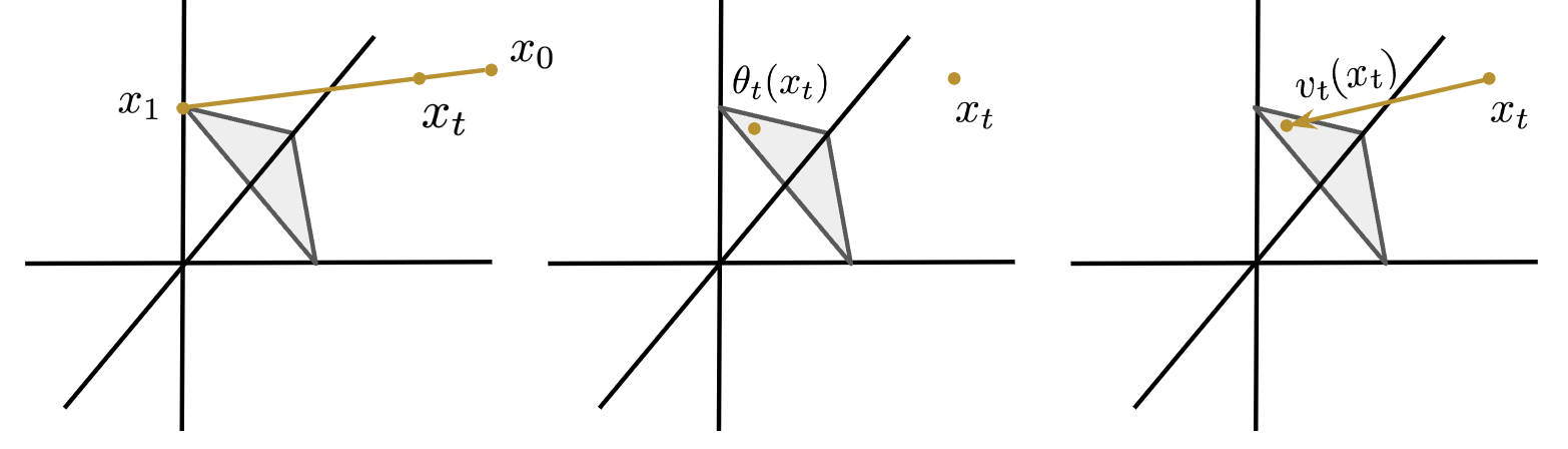
Figure 1: Reparameterized velocities by CatFlow. Note that as $\theta_{t}(x_{t})$ lies in the probability simplex, indeed all velocity implicitly are given the inductive bias of point towards it.

3.3 CatFlow: Mean-Field Variational Flow Matching for Categorical Data

The CatFlow Objective

In CatFlow, we directly apply the VFM framework to the categorical case. Let our parameterised variational distribution $q^{\theta}_{t}(x_{1}^{d}\mid x)=\mathsf{Cat}(x^{d}_{1}\mid\theta_{t}^{d}(x))$, and let us denote $\theta_{t}^{dk}(x):=q_{t}(x_{1}^{d}=k\mid x)$ for brevity. Then, the $d$th component of the learned vector field is

$$v_{t}^{\theta,d}(x):=\sum_{k=1}^{K_{d}}\theta^{dk}_{t}(x)\frac{\mathbb{I}[x_{1}^{d}=k]-x}{1-t}$$ (17)

Intuitively, CatFlow learns a distribution over the conditional trajectories to all corners of the probability simplices, rather than regressing towards an expected conditional trajectory.

In the categorical setting, the MF-VFM objective can be written out explicitly. Writing out the probability mass function of the categorical distribution, we see that

$$\log q_{t}^{\theta}(x_{1}^{d}\mid x)=\log\prod_{k=1}^{K^{d}}(\theta_{t}^{dk}(x))^{\mathbb{I}[x_{1}^{d}=k]}=\sum_{d=1}^{D}\mathbb{I}[x_{1}^{d}=k]\log\theta_{t}^{dk}(x).$$ (18)

As such, we find that CatFlow objective is given by a standard cross-entropy loss:

$$\mathcal{L}_{\text{CatFlow}}(\theta)=-\mathbb{E}_{t,x,x_{1}}\left[\sum_{d=1}^{D}\sum_{k=1}^{K^{d}}\mathbb{I}[x_{1}^{d}=k]\log\theta^{dk}_{t}(x)\right].$$ (19)

Note, however, that when actually computing $v_{t}^{\theta}$, this can be done efficiently, since

$$\mathbb{E}_{q_{t}^{\theta}(x_{1}^{d}\mid x)}\left[u_{t}(x^{d}\mid x_{1}^{d})\right]=\mathbb{E}_{q_{t}^{\theta}(x_{1}^{d}\mid x)}\left[\frac{x_{1}^{d}-x^{d}}{1-t}\right]=\frac{\theta^{d}(x)-x^{d}}{1-t},$$ (20)

since $\theta^{d}(x):=\mathbb{E}_{q_{t}^{\theta}(x_{1}^{d}\mid x)}[u_{t}^{d}(x_{1}^{d}\mid x)]$ and the other terms are not in the expectation. Note that this geometrically corresponds to learning the mapping to a point in the probability simplex, and then flowing towards that. This procedure is illustrated in fig. 1. Because of this, training CatFlow is no less efficient than flow matching.

More precisely, training CatFlow offers three key benefits over standard flow matching. First, the added inductive bias ensures generative paths align with realistic trajectories, improving performance and convergence by avoiding misaligned paths. Second, using cross-entropy loss instead of mean-squared error improves gradient behavior during training, enhancing learning dynamics and speeding up convergence. Lastly, CatFlow’s ability to learn probability vectors, rather than directly choosing classes, allows it to express uncertainty about variables at a specific time. This is especially useful in complex domains like molecular generation, where initial uncertainty about components decreases as more structure is established, leading to more precise predictions.

Permutation Equivariance.

Graphs, defined by vertices and edges, lack a natural vertex order unlike other data types. This permutation invariance means any vertex labeling represents the same graph if the connections remain unchanged. Note that even though the following results apply to graphs, an unordered set of categorical variables can be described by a graph without edges. Under natural conditions – see appendix A – we ensure CatFlow adheres to this symmetry (see section A.4 for the proof).

Theorem 2.

CatFlow generates exchangeable distributions, i.e. CatFlow generates all graph permutations with equal probability.

4 Flow Matching and Score Matching: Bridging the Gap

In this section, we relate the VFM framework to existing generative modeling approaches. First, we show that VFM has standard flow matching as a special case when the variational approximation is Gaussian. This implies that VFM provides a more general approach to learning CNFs. Second, we show that through VFM, we are not only able to compute the target vector field, but also the score function as used in score-based diffusion. This has two primary theoretical implications: 1) VFM simultaneously learns deterministic and stochastic dynamics – as diffusion models rely on stochastic dynamics, and 2) VFM provides a variational bound on the model likelihood.

Relationship to Flow Matching.

Informally, the following theorem states that VFM has flow matching as a special case when the variational approximation is Gaussian and under certain assumptions on $u_{t}(x\mid x_{1})$. This result is key, as it shows that indeed optimizing a model through VFM is more flexible than regular flow matching. Formally, the following holds (see theorem 3 in section A.2 for the proof):

Theorem 3.

Assume the conditional vector field $u_{t}(x\mid x_{1})$ is linear in $x_{1}$ and is of the form

$$u_{t}(x|x_{1})=A_{t}(x)x_{1}+b_{t}(x),$$ (21)

where $A_{t}(x):[0,1]\times\mathbb{R}^{D}\rightarrow\mathbb{R}^{D}\times\mathbb{R}^{D}$ and $b_{t}(x):[0,1]\times\mathbb{R}^{D}\rightarrow\mathbb{R}^{D}$. Moreover, assume that $A_{t}(x)$ is an invertible matrix and $q_{t}^{\theta}(x_{1}\mid x)=\mathcal{N}(x_{1}\mid\mu_{t}^{\theta}(x),\Sigma_{t}(x))$, where $\Sigma_{t}(x)=\frac{1}{2}(A^{\top}_{t}(x)A_{t}(x))^{-1}$. Then, VFM reduces to flow matching.

Relationship to Score-Based Models.

Flow matching [24] is inspired by score-based models [46] and shares strong connections with them. In score-based models, the objective is to approximate the score function $\nabla_{x}\log p_{t}(x)$ with a function $s^{\theta}_{t}(x)$. A connection to VFM becomes apparent by observing that the score function can also be expressed as an expectation with respect to $p_{t}(x_{1}\mid x)$ (see section A.5 for derivation):

$$\nabla_{x}\log p_{t}(x) =\int p_{t}(x_{1}\mid x)\nabla_{x}\log p_{t}(x\mid x_{1})\mathrm{d}x_{1}=\mathbb{E}_{p_{t}(x_{1}\mid x)}\left[\nabla_{x}\log p_{t}(x\mid x_{1})\right],$$ (22)

where $\nabla_{x}\log p_{t}(x\mid x_{1})$ is the tractable conditional score function. Similarly, we can parameterize $s^{\theta}_{t}(x)$ in terms of an expectation with respect to a variational approximation $q^{\theta}_{t}(x_{1}\mid x)$,

$$s_{t}^{\theta}(x):=\int q_{t}^{\theta}(x_{1}\mid x)\nabla_{x}\log p_{t}(x\mid x_{1})\>\mathrm{d}x_{1}.$$ (23)

It is now clear that $s_{t}^{\theta}(x)=\nabla_{x}\log p_{t}(x)$ when $q_{t}^{\theta}(x_{1}\mid x)=p_{t}(x_{1}\mid x)$. This suggests that there exists a variational formulation of score-based models that is entirely analogous to VFM. More specifically, we see that both models could be optimized using a single objective, which yields an approximation $q_{t}^{\theta}(x_{1}\mid x)$ that parameterizes both $v_{t}^{\theta}(x)$ and $s^{\theta}_{t}(x)$.

Following [46, 3], we can construct stochastic generative dynamics $dx=\tilde{v}_{t}^{\theta}(x)dt+g_{t}dw$ to approximate the true dynamics $dx=\tilde{u}_{t}(x)dt+g_{t}dw$ (see details in section A.6), with

$$\tilde{u}_{t}(x) :=\mathbb{E}_{p_{t}(x_{1}|x)}\left[u_{t}(x\mid x_{1})+\frac{g_{t}^{2}}{2}\nabla_{x}\log p_{t}(x\mid x_{1})\right], \tilde{v}^{\theta}_{t}(x) :=v_{t}^{\theta}(x)+\frac{g_{t}^{2}}{2}s_{t}^{\theta}(x).$$ (24)

Here $g_{t}:[0,1]\rightarrow\mathbb{R}_{+}$ is a scalar function, and $w$ is a standard Wiener process.

This connection has two important implications. First, it shows that learning a variational approximation $q^{\theta}_{t}(x_{1}\mid x)$ can be used to define both deterministic and stochastic dynamics, whereas flow matching typically considers deterministic dynamics only (as flows are viewed through the lens of ODEs). Second, it enables us to show that a reweighted version of the VFM objective provides a bound on the log-likelihood of the model. This bound provides another theoretical motivation for learning using the VFM objective.

Theorem 4.

Rewrite the Variational Flow Matching objective as follows:

$$\mathcal{L}_{\text{VFM}}(\theta)=\mathbb{E}_{t,x}\left[\mathcal{L}^{\theta}(t,x)\right]\quad\textrm{where}\quad\mathcal{L}^{\theta}(t,x)=-\mathbb{E}_{x_{1}}\left[\log q_{t}^{\theta}(x_{1}\mid x)\right].$$ (25)

Then, the following holds:

$$-\mathbb{E}_{x_{1}}\left[\log q_{1}^{\theta}(x_{1})\right]\leq\mathbb{E}_{t,x}\left[\lambda_{t}(x)\mathcal{L}^{\theta}(t,x)\right]+C,$$ (26)

where $\lambda_{t}(x)$ is a non-negative function and $C$ is a constant.

We provide a proof in section A.7. We further note that that applying the same linearity condition that we discussed in section 3.2 to the conditional score function maintains all the same connections with score-based models.

5 Related Work

Diffusion Models for Discrete Data.

Several approaches to discrete generation using diffusion models have been developed [4, 28, 53, 17]. For graph generation specifically, [50] utilize a Markov process that progressively edits graphs by adding or removing edges and altering node or edge categories and is trained using a graph transformer network, that reverses this process to predict the original graph structure from its noisy version. This approach breaks down the complex task of graph distribution learning into simpler node and edge classification tasks. Moreover, [19] proposes a score-based generative model for graph generation using a system of stochastic differential equations (SDEs). The model effectively captures the complex dependencies between graph nodes and edges by diffusing both node features and adjacency matrices through continuous-time processes. These are non-autoregressive graph generation approaches that perform on par with autoregressive ones, such as in [26, 23, 31]. Other non-autoregressive approaches worth mentioning are [25, 29, 28].

Flow-based methods for Discrete Data.

Very recently two flow-based methods for discrete generative modeling have been proposed, which differ both in terms of technical approach and intended use case from the work that we present here.

In [48], a Dirichlet flow framework for DNA sequence design is introduced, utilizing a transport problem defined over the probability simplex. This approach differs from CatFlow in that it represents the conditional probability path $p_{t}(x\mid x_{1})$ using a Dirichlet distribution. This implies that points $x$ are constrained to the simplex, which is not the case for CatFlow. Dirichlet Flows have not been evaluated on graph generation, but we did carry out preliminary experiments based on released source code. We have opted not to report these results; we did not obtain good performance out of the box, but have also not invested substantial time in architecture and hyperparameter selection.

In [6], Discrete Flow Models (DFMs) are introduced. DFMs use Continuous-Time Markov Chains to enable flexible and dynamic sampling in multimodal generative modeling of both continuous and discrete data. Though sharing a goal, this approach differs significantly from CatFlow as in the end the resulting model does not learn a CNF, but rather generation through sequential sampling from a time-dependent categorical distribution. As in the case of Dirichlet flows, no evaluation on graph generation was performed.

The switch to the variational perspective is inspired by [50], showing significant improvement through viewing the dynamics as a classification task over end points. However, CatFlow is still a continuous model, and integrates – rather than iteratively samples – during generation.

Table 1: Results abstract graph generation.

	Ego-small			Community-small
	Degree $\downarrow$	Clustering $\downarrow$	Orbit $\downarrow$	Degree $\downarrow$	Clustering $\downarrow$	Orbit $\downarrow$
GraphVAE	0.130	0.170	0.050	0.350	0.980	0.540
GNF	0.030	0.100	0.001	0.200	0.200	0.110
EDP-GNN	0.052	0.093	0.007	0.053	0.144	0.026
GDSS	0.021	0.024	0.007	0.045	0.086	0.007
CatFlow	0.013	0.024	0.008	0.018	0.086	0.007

6 Experiments

We evaluate CatFlow in three sets of experiments. First, we consider an abstract graph generation task proposed in [30], where the goal of this task is to evaluate if CatFlow is able to capture the topological properties of graphs. Second, we consider two common molecular benchmarks, QM9 [34] and ZINC250k [18], consisting of small and (relatively) large molecules respectively. This task is chosen to see if CatFlow can learn semantic information in graph generation, such as molecular properties. Finally, we perform an ablation comparing CatFlow to standard flow matching, specifically in terms of generalization. The experimental setup and model choices are provided in appendix C.

Note that we treat graphs as purely categorical/discrete objects and do not consider ‘geometric’ graphs that are embedded in e.g. Euclidean space. Specifically, for some graph with $K_{v}$ node classes and $K_{e}$ edge classes, we process the graph as a fully-connected graph, where each node is treated as a categorical variable of one of $K_{v}$ classes and each edge of $K_{e}+1$ classes, where the extra class corresponds with being absent.

Table 2: Results molecular generation.

	QM9			ZINC250k
	Valid $\uparrow$	Unique $\uparrow$	FCD $\downarrow$	Valid $\uparrow$	Unique $\uparrow$	FCD $\downarrow$
MoFlow	91.36	98.65	4.467	63.11	99.99	20.931
EDP-GNN	47.52	99.25	2.680	82.97	99.79	16.737
GraphEBM	8.22	97.90	6.143	5.29	98.79	35.471
GDSS	95.72	98.46	2.900	97.01	99.64	14.656
Digress	99.00	96.20	-	-	-	-
CatFlow	99.81	99.95	0.441	99.21	100.00	13.211

Figure 2: CatFlow samples of QM9 (top) and ZINC250k (bottom).

6.1 Abstract graph generation

We first evaluate CatFlow on an abstract graph generation task, including synthetic and real-world graphs. We consider 1) Ego-small (200 graphs), consisting of small ego graphs drawn from a larger Citeseer network dataset [41], 2) Community-small (100 graphs), consisting of randomly generated community graphs, 3) Enzymes (587 graphs), consisting of protein graphs representing tertiary structures of the enzymes from [40], and 4) Grid (100 graphs), consisting of 2D grid graphs. We follow the standard experimental setup popularized by [54] and hence report the maximum mean discrepancy (MMD) to compare the distributions of degree, clustering coefficient, and the number of occurrences of orbits with 4 nodes between generated graphs and a test set. Following [19], we also use the Gaussian Earth Mover’s Distance kernel to compute the MMDs instead of the total variation.

The results of the Ego-small and Community-small tasks are summarized in table 1, additional results (and error bars) are provided in appendix B. The results indicate that CatFlow is able to capture topological properties of graphs, and performs well on abstract graph generation.

6.2 Molecular Generation: QM9 & ZINC250k

Molecular generation entails designing novel molecules with specific properties, a complex task hindered by the vast chemical space and long-range dependencies in molecular structures. We evaluate CatFlow on two popular molecular generation benchmarks: QM9 and ZINC250k [34, 18].

We follow the standard setup – e.g. as in [42, 28, 50, 19] – of kekulizing the molecules using RDKit [22] and removing the hydrogen atoms. We sample 10,000 molecules and evaluate them on validity, uniqueness, and Fréchet ChemNet Distance (FCD) – evaluating the distance between data and generated molecules using the activations of ChemNet [33]. Here, validity is computed without valency correction or edge resampling, hence following [55] rather than [42, 28], as is more reasonable due to the existence of formal charges in the data itself. We do not report novelty for QM9 and ZINC250k, as QM9 is an exhaustive list of all small molecules under some chemical constraint and all models obtain (close to) 100% novelty on ZINC250k.

The results are summarized in table 2 and samples from the model are shown in fig. 2. CatFlow obtains state-of-the-art results on both QM9 and ZINC250k, virtually obtaining perfect performance on both datasets. It is worth noting that CatFlow also converges faster than flow matching and is not computationally more expensive than any of the baselines either during training or generation.

6.3 CatFlow Ablations

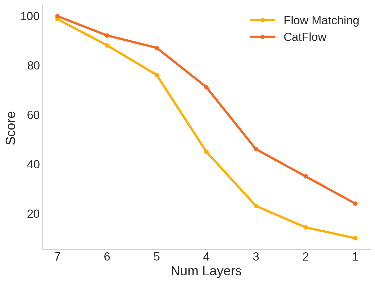
(a) Score $100\%$ of data.

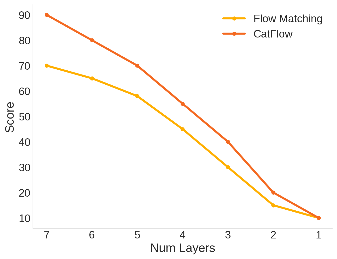
(b) Score $20\%$ of data.

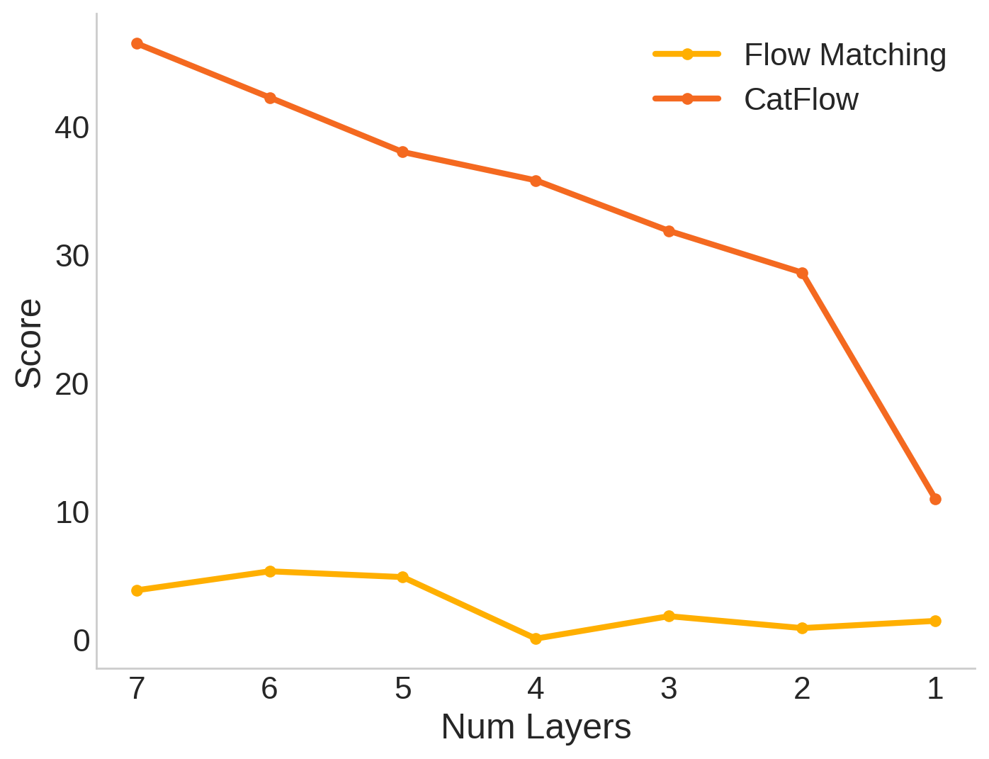
(c) Score $5\%$ of data.

Figure 3: Ablation results, comparison between standard flow matching and CatFlow.

To understand the difference in performance between CatFlow and a standard flow matching formulation we perform ablations. we focus on generalization capabilities, and as such consider ablations that the number of parameters in the model and the amount of training data.

In fig. 3 we report a score, which is the percentage of generated molecules that is valid and unique. CatFlow not only outperforms regular flow matching in the large model and full data setting, but is also significantly more robust to a decrease in model-size and data. Moreover, we observe significantly faster convergence (curves not shown). We hypothesize this is a consequence of the optimization procedure not exploring ‘irrelevant’ paths that do not point towards the probability simplex.

7 Conclusion

We have introduced a variational reformulation of flow matching. This formulation in turn informed the design of a simple flow matching method for categorical data, which achieves strong performance on graph generation tasks. Variational flow is very general and opens up several lines of inquiry. We see immediate opportunities to apply CatFlow to other discrete data types, including text, source code, and more broadly to the modeling of mixed discrete-continuous data modalities. Additionally, the connections to score-based models that we identify in this paper, suggest a path towards learning both deterministic and stochastic dynamics.

Limitations.

While the VFM formulation that we identify in this paper has potential in terms of its generality, we have as yet only considered its application to the specific task of categorical graph generation. We leave other use cases of VFM to future work. A limitation of CatFlow, which is shared with related approaches to graph generation, is that reasoning about the set of possible edges has a cost that is quadratic in the number of nodes. As a result CatFlow does not scale well to e.g. large proteins of $10^{4}$ or more atoms.

Ethics Statement.

Graph generation in general, and molecular generation specifically, holds great promise for advancing drug discovery and personalized medicine. However, this technology also poses ethical concerns, such as the potential for misuse in creating harmful substances. In terms of technology readiness, this work is not yet at a level where we foresee direct benefits or risks.

Acknowledgements

This project was supported by the Bosch Center for Artificial Intelligence.

Appendix A Proofs and Derivations

A.1 Derivation of the Variational Flow Matching Objective

We derive eq. 9 that states the equivalence of the optimization of the VFM objective and minimization of the KL divergence between the true endpoint distribution $p_{t}(x_{1}\mid x)$ and the variational approximation $q^{\theta}_{t}(x_{1}\mid x)$. Note that

$$\min_{\theta}~{}\mathbb{E}_{t,x}\left[\text{KL}\big{(}p_{t}(x_{1}\mid x)~{}||~{}q^{\theta}_{t}(x_{1}\mid x)\big{)}\right]=\max_{\theta}~{}\mathbb{E}_{t,x,x_{1}}\left[\log q_{t}^{\theta}(x_{1}\mid x)\right],$$ (27)

where $t\sim\text{Uniform}(0,1)$, $x\sim p_{t}(x)$ and $x_{1}\sim p_{\text{data}}(x_{1})$.

First, we rewrite the KL divergence as combination of entropy and cross-entropy $\text{KL}\left(p~{}||~{}q\right)=\text{H}(p,q)-\text{H}(p)$:

$$\mathbb{E}_{t,x}\left[\text{KL}\big{(}p_{t}(x_{1}\mid x)~{}||~{}q^{\theta}_{t}(x_{1}\mid x)\big{)}\right]= \mathbb{E}_{t,x}\left[\text{H}\big{(}p_{t}(x_{1}\mid x),q^{\theta}_{t}(x_{1}\mid x)\big{)}\right]-$$ (28)

$$\mathbb{E}_{t,x}\left[\text{H}\big{(}p_{t}(x_{1}\mid x)\big{)}\right].$$ (29)

We observe that the entropy term does not depend on the parameters $\theta$. Consequently we disregard it when optimising the variational distribution $q^{\theta}_{t}(x_{1}\mid x)$.

Second, we rewrite the cross-entropy term:

$$\mathbb{E}_{t,x}\left[\text{H}\big{(}p_{t}(x_{1}\mid x),q^{\theta}_{t}(x_{1}\mid x)\big{)}\right]=-\mathbb{E}_{t,x,x_{1}}\left[\log q_{t}^{\theta}(x_{1}\mid x)\right].$$ (30)

Therefore, the second part of eq. 27 corresponds to negative cross-entropy and minimisation corresponds to maximisation of negative cross-entropy.

A.2 Flow Matching as a Special Case of Variational Flow Matching

See 3

Proof.

Let us substitute the assumed form of $q_{t}^{\theta}(x_{1}\mid x)$ into the VFM objective:

$$\mathcal{L}_{\text{VFM}}(\theta) =-\mathbb{E}_{t,x,x_{1}}\left[\log q_{t}^{\theta}(x_{1}\mid x)\right]$$ (31)

$$=-\mathbb{E}_{t,x,x_{1}}\left[\log\left(\left(2\pi\right)^{-D/2}\left|\Sigma_{t}(x)\right|^{-1/2}\exp\left(-\left\|A_{t}(x)\left(x_{1}-\mu_{t}^{\theta}(x)\right)\right\|_{2}^{2}\right)\right)\right]$$ (32)

$$=\mathbb{E}_{t,x,x_{1}}\left[\left\|A_{t}(x)\left(x_{1}-\mu_{t}^{\theta}(x)\right)\right\|_{2}^{2}\right]+\frac{1}{2}\mathbb{E}_{t,x,x_{1}}\Big{[}D\log\left(2\pi\right)+\log\left|\Sigma_{t}(x)\right|\Big{]}$$ (33)

$$=\mathbb{E}_{t,x,x_{1}}\left[\left\|\left(A_{t}(x)x_{1}+b_{t}(x)\right)-\left(A_{t}(x)\mu_{t}^{\theta}(x)+b_{t}(x)\right)\right\|_{2}^{2}\right]+C$$ (34)

$$=\mathbb{E}_{t,x,x_{1}}\left[\left\|u_{t}(x\mid x_{1})-v_{t}^{\theta}(x)\right\|_{2}^{2}\right]+,$$ (35)

which is what we wanted to show. ∎

A.3 Decomposition of the Flow

See 1

Proof.

Applying the linearity condition, we rewrite the conditional vector field $u_{t}(x|x_{1})$ as such:

$$u_{t}(x\mid x_{1})=A_{t}(x)x_{1}+b_{t}(x),$$ (36)

where $A_{t}(x):[0,1]\times\mathbb{R}^{D}\rightarrow\mathbb{R}^{D}\times\mathbb{R}^{D}$ and $b_{t}(x):[0,1]\times\mathbb{R}^{D}\rightarrow\mathbb{R}^{D}$. Then, we substitute it into equation:

$$\mathbb{E}_{p_{t}(x_{1}\mid x)}\left[u_{t}(x\mid x_{1})\right] =\mathbb{E}_{p_{t}(x_{1}\mid x)}\left[A_{t}(x)x_{1}+b_{t}(x)\right]$$ (37)

$$=A_{t}(x)\mathbb{E}_{p_{t}(x_{1}\mid x)}\left[x_{1}\right]+b_{t}(x).$$ (38)

Then, we know, that for any distribution $r$ such that the marginal distributions coincide with those of $p$ the following holds:

$$\mathbb{E}_{r}[x]=\mathbb{E}_{p}[x].$$ (39)

Applying this fact to eq. 38 we obtain:

$$\mathbb{E}_{p_{t}(x_{1}\mid x)}\left[u_{t}(x\mid x_{1})\right] =A_{t}(x)\mathbb{E}_{r_{t}(x_{1}\mid x)}\left[x_{1}\right]+b_{t}(x)$$ (40)

$$=\mathbb{E}_{r_{t}(x_{1}\mid x)}\left[A_{t}(x)x_{1}+b_{t}(x)\right]$$ (41)

$$=\mathbb{E}_{r_{t}(x_{1}\mid x)}\left[u_{t}(x\mid x_{1})\right],$$ (42)

which is what we wanted to show.∎

A.4 CatFlow

Let $\mathcal{G}=(\mathcal{V},\mathcal{E})$ be a graph with node and edge features given by $\mathbf{H}_{n}\in\mathbb{R}^{|\mathcal{V}|\times d_{n}}$ and $\mathbf{H}_{e}\in\mathbb{R}^{|\mathcal{V}|\times|\mathcal{V}|\times d_{e}}$ respectively, and let $x$ denote the graphs and its features. Moreover, let $\pi\in S_{|\mathcal{V}|}$ be a permutation and $\mathbf{P}$ its associated permutation matrix, such that the action of the group is defined as

• $\pi\cdot\mathbf{H}_{n}:=\mathbf{P}\mathbf{H}_{n}$,

• $\pi\cdot\mathbf{H}_{e}:=\mathbf{P}\mathbf{H}_{e}\mathbf{P}^{\top}$.

To simplify notation, we will simply write $\pi\cdot x$ to denote the above operation.

Lemma 1.

If $\theta_{t}(x)$ is permutation equivariant w.r.t $S_{|\mathcal{V}|}$, then so is $v_{t}$.

Proof.

Note that

$$v_{t}(\pi\cdot x)=\frac{\theta_{t}(\pi\cdot x)-\pi\cdot x}{1-t}=\frac{\pi\cdot\theta_{t}(x)-\pi\cdot x}{1-t},$$

where the last step follows from permutation equivariance. Moreover, since $\pi$ acts on $x$ through permutation matrices, we can leverage the distributive property of linear operators, i.e. we conclude that

$$\frac{\pi\cdot\theta_{t}(x)-\pi\cdot x}{1-t}=\pi\cdot\frac{(\theta_{t}(x)-x)}{1-t}=\pi\cdot v_{t}(x),$$

finishing the proof.∎

Theorem 5.

Let $p_{0}$ be an exchangeable distribution – e.g. a standard normal distribution – and $\theta_{t}(x)$ be permutation equivariant. Then, all permutations of graphs are generated with equal probability.

Proof.

By result 1, we know that $\theta_{t}(x)$ being permutation equivariant implies that $v_{t}(x)$ is permutation equivariant. Moreover, if we let $\Gamma(x):=x+\int_{0}^{1}v_{t}(x_{t})dt$, the for all $\pi\in S_{n}$ we have that

$$\Gamma(\pi\cdot x)=\pi\cdot x+\int_{0}^{1}v_{t}(\pi\cdot x_{t})dt=\pi\cdot x+\int_{0}^{1}\pi\cdot v_{t}(x_{t})dt=\pi\cdot\Gamma(x),$$

where again the last step follows by basic properties of linear operators. Therefore, since $p_{0}$ assigns equal density of all permutations of $x$, the resulting distribution $p_{1}$ preservers this property, which is what we wanted to show.∎

A.5 Derivation of the Score Function

In this subsection we want to derive the equation that allows us to express the score function $\nabla_{x}\log p_{t}(x)$ in terms of the posterior probability path $p_{t}(x\mid x_{1})$. Notice that

$$\nabla_{x}\log p_{t}(x) =\frac{1}{p_{t}(x)}\nabla_{x}p_{t}(x)$$ (43)

$$=\frac{1}{p_{t}(x)}\nabla_{x}\int p_{t}(x\mid x_{1})p(x_{1})dx_{1}$$ (44)

$$=\frac{1}{p_{t}(x)}\int p(x_{1})\nabla_{x}p_{t}(x\mid x_{1})dx_{1}$$ (45)

$$=\int\frac{p_{t}(x\mid x_{1})p(x_{1})}{p_{t}(x)}\nabla_{x}\log p_{t}(x\mid x_{1})dx_{1}$$ (46)

$$=\int p_{t}(x_{1}\mid x)\nabla_{x}\log p_{t}(x\mid x_{1})dx_{1}$$ (47)

$$=\mathbb{E}_{p_{t}(x_{1}\mid x)}\left[\nabla_{x}\log p_{t}(x\mid x_{1})\right].$$ (48)

A.6 Stochastic Dynamics with Variational Flow Matching

In this subsection, we discuss how the VFM framework can be applied to construct stochastic generative dynamics and how it relates to score-based models.

First, let us consider the marginal vector field $u_{t}(x)$. It provides the deterministic dynamic that can be written as the following ordinary differential equation (ODE):

$$dx=u_{t}(x)dt.$$ (49)

For the vector field $u_{t}(x)$ we know that – starting from the distribution $p_{0}(x)$ – it generates some probability path $p_{t}(x)$. However, as we know from [46, 3], if we have access to the score function $\nabla_{x}\log p_{t}(x)$ of distribution $p_{t}(x)$, we can construct a stochastic differential equation (SDE) that, staring from distribution $p_{0}(x)$, generates the same probability path $p_{t}(x)$:

$$dx=\left[u_{t}(x)+\frac{g_{t}^{2}}{2}\nabla_{x}\log p_{t}(x)\right]dt+g_{t}dw,$$ (50)

where $g:\mathbb{R}\rightarrow\mathbb{R}_{\geq 0}$ is a scalar function, and $w$ is a standard Wiener process.

Given that

$$u_{t}(x)=\mathbb{E}_{p_{t}(x_{1}\mid x)}\left[u_{t}(x\mid x_{1})\right]\quad\textrm{and}\quad\nabla_{x}\log p_{t}(x)=\mathbb{E}_{p_{t}(x_{1}\mid x)}\left[\nabla_{x}\log p_{t}(x\mid x_{1})\right],$$ (51)

we can rewrite eq. 50 in the following form:

$$dx=\tilde{u}_{t}(x)dt+g_{t}dw,\quad\textrm{where}$$ (52)

$$\tilde{u}_{t}(x)=\mathbb{E}_{p_{t}(x_{1}\mid x)}\left[\tilde{u}_{t}(x\mid x_{1})\right] \quad\textrm{and}\quad\tilde{u}_{t}(x\mid x_{1})=u_{t}(x\mid x_{1})+\frac{g_{t}^{2}}{2}\nabla_{x}\log p_{t}(x\mid x_{1}).$$ (53)

Importantly, the function $g_{t}$ does not affect the distribution path $p_{t}(x)$: it only changes the stochasticity of the trajectories. In the extreme case when $g_{t}\equiv 0$, the SDE in eq. 50 coincides with the ODE in eq. 49.

Moreover, if we construct the stochastic dynamics in this way, we obtain score-based models as a special case. In score-based models [46] the deterministic process that corresponds to probability path $p_{t}(x)$ has the following form:

$$dx=u_{t}(x)dt\quad\textrm{where}\quad u_{t}(x)=f_{t}(x)+\frac{g_{t}^{2}}{2}\nabla_{x}\log p_{t}(x),$$ (54)

where $f_{t}(x)$ is tractable. Substituting this $u_{t}(x)$ into eq. 50 we obtain:

$$dx=\left[f_{t}(x)+g_{t}^{2}\nabla_{x}\log p_{t}(x)\right]dt+g_{t}dw.$$ (55)

The SDE in eq. 55 only depends on the score function, so in score-based models, the aim is to learn the score function.

Now, let us note that similarly to vector field $u_{t}(x)$, the drift term $\tilde{u}_{t}(x)$ in eq. 52 can be expressed in terms of an end point distribution $p_{t}(x_{1}\mid x)$. Consequently, having a variational approximation of end point distribution $q_{t}^{\theta}(x_{1}\mid x)$, allows us to construct an approximation of the drift term $\tilde{u}_{t}(x)$:

$$\tilde{v}^{\theta}_{t}(x)=\mathbb{E}_{q_{t}^{\theta}(x_{1}\mid x)}\left[\tilde{u}_{t}(x\mid x_{1})\right] =v^{\theta}_{t}(x)+\frac{g_{t}^{2}}{2}s^{\theta}_{t}(x),$$ (56)

$$\textrm{where}\quad v^{\theta}_{t}(x)=\mathbb{E}_{q_{t}^{\theta}(x_{1}\mid x)}\left[u_{t}(x\mid x_{1})\right]\quad\textrm{and}\quad s^{\theta}_{t}(x)=\mathbb{E}_{q_{t}^{\theta}(x_{1}\mid x)}\left[\nabla_{x}\log p_{t}(x\mid x_{1})\right].$$ (57)

Thus, we may define the following approximated SDE:

$$dx=\tilde{v}^{\theta}_{t}(x)dt+g_{t}dw\quad\textrm{or}\quad dx=\left[v^{\theta}_{t}(x)+\frac{g_{t}^{2}}{2}s^{\theta}_{t}(x)\right]dt+g_{t}dw.$$ (58)

Then, eq. 58 is not just simply a new dynamic, it is a family of dynamics that admits deterministic dynamics as a special case when $g_{t}\equiv 0$. Importantly, the only thing we need to construct the stochastic process in eq. 58 is an approximation of the end point distributions $q_{t}^{\theta}(x_{1}\mid x)$. Additionally we know that when $p_{t}(x_{1}\mid x)=q_{t}^{\theta}(x_{1}\mid x)$, $\tilde{u}_{t}(x)=\tilde{v}^{\theta}_{t}(x)$, the processes coincide for all functions $g_{t}$. Therefore, we can train the model with the same objective as in VFM.

A.7 Variational Flow Matching as a Variational Bound on the Log-likelihood

In this subsection, we leverage the connections of VFM with stochastic processes to show that a reweighted integral over the point-wise VFM objective defines a bound on the data likelihood in the generative model.

See 4

Proof.

Let us consider the two stochastic processes, that we discussed in section A.6:

$$dx=\tilde{u}_{t}(x)dt+g_{t}dw,\quad\textrm{where}\quad dx=\tilde{v}^{\theta}_{t}(x)dt+g_{t}dw.$$ (59)

Note that they both start from the same prior distribution $p_{0}(x)$. The first one, by design, generates probability path $p_{t}(x)$ and ends up in the data distribution $p_{\text{data}}(x)=p_{1}(x)$. The second process generates some probability path $q^{\theta}_{t}(x)$ that depends on the variational distribution $q^{\theta}_{t}(x_{1}|x)$.

We want to find a variational bound on KL divergence between $p_{1}(x)$ and $q^{\theta}_{1}(x)$. We start by applying the result from [1] (see Lemma 2.22):

$$\text{KL}\left(p_{1}(x_{1})\|q^{\theta}_{1}(x_{1})\right) \leq\mathbb{E}_{t,x}\left[\frac{1}{2g_{t}^{2}}\left\|\tilde{u}_{t}(x)-\tilde{v}^{\theta}_{t}(x)\right\|_{2}^{2}\right]$$ (60)

$$=\mathbb{E}_{t,x}\left[\frac{1}{2g_{t}^{2}}\left\|\int\left(p_{t}(x_{1}\mid x)-q^{\theta}_{t}(x_{1}\mid x)\right)\tilde{u}_{t}(x|x_{1})dx_{1}\right\|_{2}^{2}\right]$$ (61)

$$\leq\mathbb{E}_{t,x}\left[\frac{1}{2g_{t}^{2}}\left(\int\Big{\|}\left(p_{t}(x_{1}\mid x)-q^{\theta}_{t}(x_{1}\mid x)\right)\tilde{u}_{t}(x|x_{1})\Big{\|}dx_{1}\right)^{2}\right]$$ (62)

$$\leq\mathbb{E}_{t,x}\left[\frac{1}{2g_{t}^{2}}\left(\int\left|p_{t}(x_{1}\mid x)-q^{\theta}_{t}(x_{1}\mid x)\right|\left\|\tilde{u}_{t}(x|x_{1})\right\|dx_{1}\right)^{2}\right].$$ (63)

Now, let us introduce two auxiliary functions:

$$l_{t}(x)=\sup_{x_{1}}\left\|\tilde{u}_{t}(x|x_{1})\right\|\quad\textrm{and}\quad\lambda_{t}(x)=\frac{l_{t}(x)}{g_{t}^{2}}.$$ (64)

If we utilise $\lambda_{t}(x)$ to write down the following bound, we see that

$$\text{KL}\left(p_{1}(x_{1})\|q^{\theta}_{1}(x_{1})\right) \leq\mathbb{E}_{t,x}\left[\frac{\lambda_{t}(x)}{2}\left(\int\left|p_{t}(x_{1}\mid x)-q^{\theta}_{t}(x_{1}\mid x)\right|dx_{1}\right)_{2}^{2}\right].$$ (65)

Next, we can apply Pinsker’s inequality, which states that for two probability distributions $p$ and $q$ the following holds:

$$\int|p(x)-q(x)|dx\leq 2\text{KL}(p\|q).$$ (66)

Applying it to the inner integral, we have:

$$\text{KL}\left(p_{1}(x_{1})\|q^{\theta}_{1}(x_{1})\right) \leq\mathbb{E}_{t,x}\left[\lambda_{t}(x)\text{KL}\Big{(}p_{t}(x_{1}\mid x)\|q^{\theta}_{t}(x_{1}\mid x)\Big{)}\right].$$ (67)

We may rewrite the left part of inequality as a combination of the data entropy and the model’s likelihood, where only the likelihood depends on parameters $\theta$:

$$\text{KL}\left(p_{1}(x_{1})\|q^{\theta}_{1}(x_{1})\right)=-\text{H}\left(p_{1}(x_{1})\right)-\mathbb{E}_{x_{1}}\left[\log q^{\theta}_{1}(x_{1})\right].$$ (68)

The right part of inequality can be rewritten as an expectation of entropy that does not depend on any parameters $\theta$ plus a reweighted VFM objective with weighting coefficient $\lambda_{t}(x)$:

$$\mathbb{E}_{t,x}\left[\lambda_{t}(x)\text{KL}\Big{(}p_{t}(x_{1}\mid x)\|q^{\theta}_{t}(x_{1}\mid x)\Big{)}\right]= -\mathbb{E}_{t,x}\left[\lambda_{t}(x)\text{H}(p_{t}(x_{1}\mid x))\right]$$ (69)

$$-\mathbb{E}_{t,x,x_{1}}\left[\lambda_{t}(x)q^{\theta}_{t}(x_{1}\mid x)\right]$$ (70)

We see that this reweighted version of the VFM objective defines an upper bound on the model likelihood, which was what we wanted to show.∎

A.8 Stochastic Dynamics under Linearity Conditions

In this subsection, we discuss the connection between VFM and stochastic dynamics under the condition of linearity in $x_{1}$ of the conditional vector field $u_{t}(x\mid x_{1})$ and conditional score function $\nabla_{x}\log p_{t}(x\mid x_{1})$.

As we discuss in section 3.2, under the linearity condition, we may express $u_{t}(x)$ in terms of any distribution of end points $r_{t}(x_{1}\mid x)$ if it has the same marginals as $p_{t}(x_{1}\mid x)$. In section A.5, we demonstrate that the score function $\nabla_{x}\log p_{t}(x)$ can also be expressed in terms of end point distributions $p_{t}(x_{1}\mid x)$. Therefore, the score function may also be equally expressed in terms of distribution $r_{t}(x_{1}\mid x)$ if it has the same marginals as $p_{t}(x_{1}\mid x)$. This fact is easy to show in the same way as we present in section A.3.

Consequently, under the linearity conditions, the drift term $\tilde{u}_{t}(x)$ can also be expressed in terms of $r_{t}(x_{1}\mid x)$, as it is just a linear combination of the vector field $u_{t}(x)$ and score function $\nabla_{x}\log p_{t}(x)$. Hence, the transition from the distribution $p_{(}x_{1}\mid x)$ to some distribution $r_{(}x_{1}\mid x)$ does not affect the discussion of connections of stochastic dynamics in section A.6.

Furthermore, the transition from distribution $p_{t}(x_{1}\mid x)$ to some distribution $r_{t}(x_{1}\mid x)$ does not affect connections of the VFM objective with the model likelihood that we discuss in section A.7. It is easy to see that in the derivations, we only rely on functions $\tilde{u}_{t}(x)$ and $\tilde{v}^{\theta}_{t}(x)$ (see eq. 60). However, as we discussed, they are not affected by the transition from $p_{t}(x_{1}\mid x)$ to some $r_{t}(x_{1}\mid x)$. Therefore, we may repeat all the same derivations for some $r_{(}x_{1}|x)$ using a factorized distribution.

Appendix B Detailed Results

Here, we provide the results for CatFlow with standard deviations, as computed as in [19] through multiple seeds.

Ego-small			Community-small
$4\leq|\mathcal{V}|\leq 18$			$12\leq|\mathcal{V}|\leq 20$
Degree $\downarrow$	Clustering $\downarrow$	Orbit $\downarrow$	Degree $\downarrow$	Clustering $\downarrow$	Orbit $\downarrow$
$0.013\pm 0.007$	$0.024\pm 0.009$	$0.008\pm 0.005$	$0.018\pm 0.012$	$0.086\pm 0.021$	$0.007\pm 0.005$

Enzymes			Grid
$10\leq|\mathcal{V}|\leq 125$			$100\leq|\mathcal{V}|\leq 400$
Degree $\downarrow$	Clustering $\downarrow$	Orbit $\downarrow$	Degree $\downarrow$	Clustering $\downarrow$	Orbit $\downarrow$
$0.013\pm 0.012$	$0.062\pm 0.011$	$0.008\pm 0.007$	$0.115\pm 0.010$	$0.004\pm 0.002$	$0.075\pm 0.071$

QM9			ZINC250k
$1\leq|\mathcal{V}|\leq 9$, 4 atom types			$6\leq|\mathcal{V}|\leq 38$, 9 atom types
Valid $\uparrow$	Unique $\uparrow$	FCD $\downarrow$	Valid $\uparrow$	Unique $\uparrow$	FCD $\downarrow$
$99.81\pm 0.03$	$99.95\pm 0.02$	$0.441\pm 0.023$	$99.21\pm 0.04$	$100.00\pm 0.00$	$13.211\pm 0.12$

Appendix C Experimental setup

C.1 Model

To ensure a comparison on equal terms to baselines, we employ the same graph transformer network as proposed in [11], which was also used in [50], along with the same hyper-parameter setup. We summarize the parametrization of our network here.

Just as done in DiGress, our graph transformer takes as input a graph $(\mathbf{H}_{n},\mathbf{H}_{e})$ and predicts a distribution over the clean graphs, using structural and spectral features to improve the network expressivity, which we denote as $\mathbf{H}_{g}$. Each transformer layer does the following operations:

1. Node Features $\mathbf{H}_{n}$ and Edge Features $\mathbf{H}_{e}$:

   1. Linear Transformation: Apply linear transformations to both $\mathbf{H}_{n}$ and $\mathbf{H}_{e}$.

   2. Outer Product and Scaling: Compute the outer product of the transformed features and apply scaling.

2. Node Features $\mathbf{H}_{n}$:

   1. Feature-wise Linear Modulation (FiLM): Apply FiLM to the transformed node features using global features $\mathbf{H}_{g}$.

3. Edge Features $\mathbf{H}_{e}$:

   1. Feature-wise Linear Modulation (FiLM): Apply FiLM to the transformed edge features using global features $\mathbf{H}_{g}$.

4. Self-Attention Mechanism:

   1. Linear Transformation: Apply a linear transformation to the transformed node features.

   2. Softmax Operation: Compute the attention scores using the softmax function.

   3. Attention Score Calculation: Calculate the weighted sum of the transformed node features based on the attention scores.

5. Global Features $y$:

   1. Pooling: Apply PNA pooling to the node features $\mathbf{H}_{n}$ and edge features $\mathbf{H}_{e}$.

   2. Summation: Sum the pooled features with the global features $\mathbf{H}_{g}$.

6. Final Outputs:

   1. Node Features $\mathbf{H}_{n}^{\prime}$: Obtain updated node features after the attention mechanism.

   2. Edge Features $\mathbf{H}_{e}^{\prime}$: Obtain updated edge features after the attention mechanism.

   3. Global Features $\mathbf{H}_{g}^{\prime}$: Obtain updated global features after summation.

Here, the FiLM operation is defined as:

$$\text{FiLM}(M_{1},M_{2})=M_{1}W_{1}+(M_{1}W_{2})\odot M_{2}+M_{2}$$

for learnable weight matrices $W_{1}$ and $W_{2}$, and PNA is defined as:

$$\text{PNA}(X)=\text{cat}(\text{max}(X),\text{min}(X),\text{mean}(X),\text{std}(X))W.$$

C.2 Hyperparameters and Computational Costs

We report the hyperparameters here:

Hyperparameter	Abstract	QM9/ZINC250k	Ablation
Optimizer	AdamW	AdamW	AdamW
Scheduler	Cosine Annealing	Cosine Annealing	Cosine Annealing
Learning Rate	$2\cdot 10^{-4}$	$2\cdot 10^{-4}$	$2\cdot 10^{-4}$
Weight Decay	$1\cdot 10^{-12}$	$1\cdot 10^{-12}$	$1\cdot 10^{-12}$
EMA	0.999	0.999	0.999

Table 3: Hyperparameter setup.

All models were trained until convergence. Furthermore, all data splits are kept the same as in [19], and hidden dimensions are kept the same as [50]. All experiments were run on a single NVIDIA RTX 6000 and took about a day to run.

Appendix D Detail CNFs

To compute the resulting distribution $p_{t}$ for CNF, one can use the change of variables formula:

$$[\varphi_{t}]_{*}p_{0}(x)=p_{0}(\varphi_{t}^{-1}(x))\text{det}\left[\frac{\partial\varphi_{t}^{-1}}{\partial x}(x)\right].$$ (71)

This induces a probability path, i.e. a mapping $p_{t}:[0,1]\times\mathbb{R}^{D}\to\mathbb{R}_{>0}$ such that $\int p_{t}(x)dx=1$ for all $t\in[0,1]$. We say that $v_{t}$ generates this probability path given a starting distribution $p_{0}$. In theory, one could try and optimize the empirical divergence between the resulting distribution $p_{1}$ and target distribution, but obtaining a gradient sample for the loss requires us to solve the ODE at each step during training, making this approach computationally prohibitive.

One way to assess if a vector field generates a specific probability path is using the continuity equation, i.e. we can assess whether $v_{t}$ and $p_{t}$ satisfy

$$\frac{\partial}{\partial t}p_{t}(x)+\nabla\cdot(p_{t}(x)v_{t}(x))=0,$$ (72)

where $\nabla$ is the divergence operator. Note that by sampling $x_{0}\sim p_{0}$, a new sample from $p_{1}$ can be generated by following this ODE, i.e. integrating

$$x_{1}=x_{0}+\int_{0}^{1}v_{t}(x_{t})\mathrm{d}t.$$ (73)

References

- [1] Michael S Albergo, Nicholas M Boffi, and Eric Vanden-Eijnden. Stochastic interpolants: A unifying framework for flows and diffusions. arXiv preprint arXiv:2303.08797, 2023.
- [2] Michael Samuel Albergo and Eric Vanden-Eijnden. Building Normalizing Flows with Stochastic Interpolants. In The Eleventh International Conference on Learning Representations, September 2022.
- [3] Brian DO Anderson. Reverse-time diffusion equation models. Stochastic Processes and their Applications, 12(3):313–326, 1982.
- [4] Jacob Austin, Daniel D Johnson, Jonathan Ho, Daniel Tarlow, and Rianne Van Den Berg. Structured denoising diffusion models in discrete state-spaces. Advances in Neural Information Processing Systems, 34:17981–17993, 2021.
- [5] Heli Ben-Hamu, Samuel Cohen, Joey Bose, Brandon Amos, Maximillian Nickel, Aditya Grover, Ricky T. Q. Chen, and Yaron Lipman. Matching normalizing flows and probability paths on manifolds. In Kamalika Chaudhuri, Stefanie Jegelka, Le Song, Csaba Szepesvari, Gang Niu, and Sivan Sabato, editors, Proceedings of the 39th International Conference on Machine Learning, volume 162 of Proceedings of Machine Learning Research, pages 1749–1763. PMLR, 17–23 Jul 2022.
- [6] Andrew Campbell, Jason Yim, Regina Barzilay, Tom Rainforth, and Tommi Jaakkola. Generative flows on discrete state-spaces: Enabling multimodal flows with applications to protein co-design. arXiv preprint arXiv:2402.04997, 2024.
- [7] Ricky TQ Chen and Yaron Lipman. Flow matching on general geometries. In The Twelfth International Conference on Learning Representations, 2024.
- [8] Ricky TQ Chen, Yulia Rubanova, Jesse Bettencourt, and David K Duvenaud. Neural ordinary differential equations. Advances in neural information processing systems, 31, 2018.
- [9] Quan Dao, Hao Phung, Binh Nguyen, and Anh Tran. Flow matching in latent space. arXiv preprint arXiv:2307.08698, 2023.
- [10] Giannis Daras, Mauricio Delbracio, Hossein Talebi, Alexandros G Dimakis, and Peyman Milanfar. Soft diffusion: Score matching for general corruptions. arXiv preprint arXiv:2209.05442, 2022.
- [11] Vijay Prakash Dwivedi and Xavier Bresson. A generalization of transformer networks to graphs. arXiv preprint arXiv:2012.09699, 2020.
- [12] Ehsan Ebrahimy and Robert Shimer. Stock–flow matching. Journal of Economic Theory, 145(4):1325–1353, 2010.
- [13] Will Grathwohl, Ricky T. Q. Chen, Jesse Bettencourt, and David Duvenaud. Scalable reversible generative models with free-form continuous dynamics. In International Conference on Learning Representations, 2019.
- [14] Jonathan Ho, Ajay Jain, and Pieter Abbeel. Denoising diffusion probabilistic models. Advances in neural information processing systems, 33:6840–6851, 2020.
- [15] Emiel Hoogeboom and Tim Salimans. Blurring diffusion models. arXiv preprint arXiv:2209.05557, 2022.
- [16] Emiel Hoogeboom, Vıctor Garcia Satorras, Clément Vignac, and Max Welling. Equivariant diffusion for molecule generation in 3d. In International conference on machine learning, pages 8867–8887. PMLR, 2022.
- [17] Naoto Inoue, Kotaro Kikuchi, Edgar Simo-Serra, Mayu Otani, and Kota Yamaguchi. Layoutdm: Discrete diffusion model for controllable layout generation. In Proceedings of the IEEE/CVF Conference on Computer Vision and Pattern Recognition, pages 10167–10176, 2023.
- [18] John J Irwin, Teague Sterling, Michael M Mysinger, Erin S Bolstad, and Ryan G Coleman. Zinc: a free tool to discover chemistry for biology. Journal of chemical information and modeling, 52(7):1757–1768, 2012.
- [19] Jaehyeong Jo, Seul Lee, and Sung Ju Hwang. Score-based Generative Modeling of Graphs via the System of Stochastic Differential Equations. In Proceedings of the 39th International Conference on Machine Learning, pages 10362–10383. PMLR, June 2022.
- [20] Leon Klein, Andreas Krämer, and Frank Noe. Equivariant flow matching. In Thirty-Seventh Conference on Neural Information Processing Systems, November 2023.
- [21] Jonas Kohler, Yaoyi Chen, Andreas Kramer, Cecilia Clementi, and Frank Noé. Flow-matching: Efficient coarse-graining of molecular dynamics without forces. Journal of Chemical Theory and Computation, 19(3):942–952, 2023.
- [22] Greg Landrum. Rdkit: Open-source cheminformatics software, 2016.
- [23] Renjie Liao, Yujia Li, Yang Song, Shenlong Wang, Will Hamilton, David K Duvenaud, Raquel Urtasun, and Richard Zemel. Efficient graph generation with graph recurrent attention networks. Advances in neural information processing systems, 32, 2019.
- [24] Yaron Lipman, Ricky T. Q. Chen, Heli Ben-Hamu, Maximilian Nickel, and Matthew Le. Flow matching for generative modeling. In The Eleventh International Conference on Learning Representations, 2023.
- [25] Phillip Lippe and Efstratios Gavves. Categorical Normalizing Flows via Continuous Transformations. In International Conference on Learning Representations, October 2020.
- [26] Qi Liu, Miltiadis Allamanis, Marc Brockschmidt, and Alexander Gaunt. Constrained graph variational autoencoders for molecule design. Advances in neural information processing systems, 31, 2018.
- [27] Xingchao Liu, Chengyue Gong, and Qiang Liu. Flow straight and fast: Learning to generate and transfer data with rectified flow. In The Eleventh International Conference on Learning Representations, 2023.
- [28] Youzhi Luo, Keqiang Yan, and Shuiwang Ji. Graphdf: A discrete flow model for molecular graph generation. In International conference on machine learning, pages 7192–7203. PMLR, 2021.
- [29] Kaushalya Madhawa, Katushiko Ishiguro, Kosuke Nakago, and Motoki Abe. Graphnvp: An invertible flow model for generating molecular graphs. arXiv preprint arXiv:1905.11600, 2019.
- [30] Karolis Martinkus, Andreas Loukas, Nathanaël Perraudin, and Roger Wattenhofer. Spectre: Spectral conditioning helps to overcome the expressivity limits of one-shot graph generators. In International Conference on Machine Learning, pages 15159–15179. PMLR, 2022.
- [31] Rocío Mercado, Tobias Rastemo, Edvard Lindelöf, Günter Klambauer, Ola Engkvist, Hongming Chen, and Esben Jannik Bjerrum. Graph networks for molecular design. Machine Learning: Science and Technology, 2(2):025023, 2021.
- [32] George Papamakarios, Eric Nalisnick, Danilo Jimenez Rezende, Shakir Mohamed, and Balaji Lakshminarayanan. Normalizing flows for probabilistic modeling and inference. Journal of Machine Learning Research, 22(57):1–64, 2021.
- [33] Kristina Preuer, Philipp Renz, Thomas Unterthiner, Sepp Hochreiter, and Gunter Klambauer. Fréchet chemnet distance: a metric for generative models for molecules in drug discovery. Journal of chemical information and modeling, 58(9):1736–1741, 2018.
- [34] Raghunathan Ramakrishnan, Pavlo O Dral, Matthias Rupp, and O Anatole Von Lilienfeld. Quantum chemistry structures and properties of 134 kilo molecules. Scientific data, 1(1):1–7, 2014.
- [35] Aditya Ramesh, Prafulla Dhariwal, Alex Nichol, Casey Chu, and Mark Chen. Hierarchical text-conditional image generation with clip latents. arXiv preprint arXiv:2204.06125, 1(2):3, 2022.
- [36] Danilo Rezende and Shakir Mohamed. Variational inference with normalizing flows. In International conference on machine learning, pages 1530–1538. PMLR, 2015.
- [37] Severi Rissanen, Markus Heinonen, and Arno Solin. Generative modelling with inverse heat dissipation. arXiv preprint arXiv:2206.13397, 2022.
- [38] Robin Rombach, Andreas Blattmann, Dominik Lorenz, Patrick Esser, and Björn Ommer. High-resolution image synthesis with latent diffusion models. In Proceedings of the IEEE/CVF conference on computer vision and pattern recognition, pages 10684–10695, 2022.
- [39] Noam Rozen, Aditya Grover, Maximilian Nickel, and Yaron Lipman. Moser flow: Divergence-based generative modeling on manifolds. Advances in Neural Information Processing Systems, 34:17669–17680, 2021.
- [40] Ida Schomburg, Antje Chang, Christian Ebeling, Marion Gremse, Christian Heldt, Gregor Huhn, and Dietmar Schomburg. Brenda, the enzyme database: updates and major new developments. Nucleic acids research, 32(suppl_1):D431–D433, 2004.
- [41] Prithviraj Sen, Galileo Namata, Mustafa Bilgic, Lise Getoor, Brian Galligher, and Tina Eliassi-Rad. Collective classification in network data. AI magazine, 29(3):93–93, 2008.
- [42] Chence Shi, Minkai Xu, Zhaocheng Zhu, Weinan Zhang, Ming Zhang, and Jian Tang. Graphaf: a flow-based autoregressive model for molecular graph generation. In International Conference on Learning Representations, 2019.
- [43] Raghav Singhal, Mark Goldstein, and Rajesh Ranganath. Where to diffuse, how to diffuse and how to get back: Automated learning in multivariate diffusions. In International Conference on Learning Representations, 2023.
- [44] Jiaming Song, Chenlin Meng, and Stefano Ermon. Denoising diffusion implicit models. In International Conference on Learning Representations, 2020.
- [45] Yang Song, Conor Durkan, Iain Murray, and Stefano Ermon. Maximum likelihood training of score-based diffusion models. Advances in neural information processing systems, 34:1415–1428, 2021.
- [46] Yang Song, Jascha Sohl-Dickstein, Diederik P Kingma, Abhishek Kumar, Stefano Ermon, and Ben Poole. Score-based generative modeling through stochastic differential equations. In International Conference on Learning Representations, 2020.
- [47] Yuxuan Song, Jingjing Gong, Minkai Xu, Ziyao Cao, Yanyan Lan, Stefano Ermon, Hao Zhou, and Wei-Ying Ma. Equivariant Flow Matching with Hybrid Probability Transport for 3D Molecule Generation. In Thirty-Seventh Conference on Neural Information Processing Systems, November 2023.
- [48] Hannes Stark, Bowen Jing, Chenyu Wang, Gabriele Corso, Bonnie Berger, Regina Barzilay, and Tommi Jaakkola. Dirichlet flow matching with applications to dna sequence design. arXiv preprint arXiv:2402.05841, 2024.
- [49] Brian L Trippe, Jason Yim, Doug Tischer, David Baker, Tamara Broderick, Regina Barzilay, and Tommi S Jaakkola. Diffusion probabilistic modeling of protein backbones in 3d for the motif-scaffolding problem. In The Eleventh International Conference on Learning Representations, 2022.
- [50] Clement Vignac, Igor Krawczuk, Antoine Siraudin, Bohan Wang, Volkan Cevher, and Pascal Frossard. DiGress: Discrete Denoising diffusion for graph generation. In The Eleventh International Conference on Learning Representations, September 2022.
- [51] Pascal Vincent. A connection between score matching and denoising autoencoders. Neural computation, 23(7):1661–1674, 2011.
- [52] Jonas Wildberger, Maximilian Dax, Simon Buchholz, Stephen Green, Jakob H Macke, and Bernhard Schölkopf. Flow matching for scalable simulation-based inference. Advances in Neural Information Processing Systems, 36, 2024.
- [53] Dongchao Yang, Jianwei Yu, Helin Wang, Wen Wang, Chao Weng, Yuexian Zou, and Dong Yu. Diffsound: Discrete diffusion model for text-to-sound generation. IEEE/ACM Transactions on Audio, Speech, and Language Processing, 2023.
- [54] Jiaxuan You, Rex Ying, Xiang Ren, William Hamilton, and Jure Leskovec. Graphrnn: Generating realistic graphs with deep auto-regressive models. In International conference on machine learning, pages 5708–5717. PMLR, 2018.
- [55] Chengxi Zang and Fei Wang. Moflow: an invertible flow model for generating molecular graphs. In Proceedings of the 26th ACM SIGKDD international conference on knowledge discovery & data mining, pages 617–626, 2020.
- [56] Qinsheng Zhang and Yongxin Chen. Fast sampling of diffusion models with exponential integrator. In The Eleventh International Conference on Learning Representations, 2022.