Emergent Universe from an Unstable de Sitter Phase

Abstract

In the Emergent scenario, the Universe should evolve from a non-singular state replacing the typical singularity of General Relativity, for any initial condition. For the scalar field model in [1] we show that only a subset of initial conditions leads to emergence, either from a static state (an Einstein model), or from a de Sitter state.

Assuming a scenario based on CDM interacting with a Dark Energy fluid, we show that in general flat and open models expand from a non-singular unstable de Sitter state at high energies; for closed models this state is a transition phase with a bounce. A subset of these models are qualitatively in agreement with the observable Universe, accelerating at high energies, going through a matter-dominated decelerated era, then accelerating toward a de Sitter phase.

1 Introduction

The Standard Model of Cosmology, a flat $\Lambda$CDM model with inflation, is based on General Relativity (GR) and provides a successful framework to describe the evolution of the Universe. However, the presence of singularities pose a problem and are currently interpreted as points in space-time where GR breaks down [2, 3, 4, 5]. Observations are consistent with a flat universe [6, 7], however they do not rule out open or closed spatial curvature [8]. In particular, a closed universe is appealing as it avoids the problem of having an infinite universe [9]. The Emergent Universe has been widely studied as an alternative to an initial singularity, with models built with fine-tuned initial conditions on the assumption that the past repellor must be a static state represented by an Einstein model with positive curvature [1, 10, 11, 12, 13, 14, 15, 16, 17, 18, 19]. Thus the problem with this scenario is that very special initial conditions are required, as the Einstein model is typically represented by an unstable saddle or a centre in the phase space of the relevant Ordinary Differential Equations (ODE), and so it is not a generic past repellor, as in the classical model by Eddington [20].

In this essay we contend that in the Emergent scenario, the Universe should evolve from a non-singular state replacing the typical singularity of GR for any initial condition. In this light, we first consider whether models in [1], based on a scalar field, are still non-singular for general initial conditions. Similarly to the analysis in [21] and [22], we complete a dynamical systems analysis of the Emergent scenario in [1]. We show that only a set of measure zero of trajectories emerge from the static Einstein model. We also find a class of models that do in fact emerge from a non-singular de Sitter fixed point, representing a state where the scalar field is potential dominated. The problem with this class of models is that the stability type of this de Sitter fixed point is that of a 3-D saddle, so some fine-tuning is still required for models to be non-singular. For trajectories not emerging from this de Sitter state, we find that the past repellor is a fixed point representing a stiff fluid singularity where the scalar field is kinetic dominated.

We then consider a fluid-based model to show an example where emergence from a non-singular state is generic during expansion, regardless of initial conditions. Assuming a scenario based on Cold Dark Matter (CDM, represented by a dust fluid) interacting with a Dark Energy fluid with a nonlinear equation of state, we show that all but a set of measure zero of trajectories in phase space expand from an unstable de Sitter state, a classical vacuum at high energies. This represents the asymptotic past of flat and open models, and a transition phase with a bounce for closed models. Independently from the initial conditions, all models are accelerating at high energies. A subset of models are qualitatively in agreement with the observed universe, emerging from a non-singular state, going through a matter-dominated decelerated era, then accelerating toward the future de Sitter phase.

2 Scalar-Field-Based Emergent Universe

We consider a Friedmann-Lemaître-Robertson-Walker (FLRW) universe, containing a scalar field $\phi$ with the potential

$$V=V_{0}\left(e^{\phi}-1\right)^{2}\,,$$ (1)

where $V_{0}$ is the asymptotic value of the potential at $\phi\rightarrow-\infty$. Assuming $8\pi G=c=1$, the Klein-Gordon and Raychaudhuri equations are

$$\ddot{\phi}=-3H\dot{\phi}-2V_{0}e^{\phi}(e^{\phi}-1)\,,$$ (2)

$$\dot{H}=-H^{2}-\frac{1}{3}\left[\dot{\phi}^{2}-V_{0}(e^{\phi}-1)^{2}\right]\,,$$ (3)

where $H=\dot{a}/a$ is the Hubble expansion scalar ($a$ is the scale factor) and over-dots are derivatives with respect to time. The dynamics is complemented by the usual Friedmann first integral (the Hamiltonian constraint)

$$H^{2}=-\frac{k}{a^{2}}+\frac{1}{3}\left[\frac{\dot{\phi}^{2}}{2}+V(\phi)\right].$$ (4)

Setting $\psi=\dot{\phi}/\sqrt{V_{0}}$ defines a 3-dimensional set of ODE. To analyse this dynamical system we define dimensionless variables ($\phi$ is dimensionless by definition) and their compactified version,

$$\eta=\sqrt{V_{0}}t,~{}~{}~{}\Phi=\frac{\phi}{\sqrt{1+\phi^{2}}},~{}~{}~{}\psi=\frac{\dot{\phi}}{\sqrt{V_{0}}},~{}~{}~{}\Psi=\frac{\psi}{\sqrt{1+\psi^{2}}},~{}~{}~{}y=\frac{H}{\sqrt{V_{0}}},~{}~{}~{}Y=\frac{y}{\sqrt{1+y^{2}}}\,,$$ (5)

in order to study the behaviour of the system at infinity. Here, $\phi\rightarrow\pm\infty$ corresponds to $\Phi=\pm 1$, $\psi\rightarrow\pm\infty$ to $\Psi=\pm 1$ and $y\rightarrow\pm\infty$ to $Y=\pm 1$.

First, we consider the phase space of spatially flat models. The Friedmann equation (4) with $k=0$ in our compactified variables becomes

$$\frac{Y}{\sqrt{1-Y^{2}}}=\pm\sqrt{\frac{1}{3}\left(e^{\frac{\Phi^{2}}{\sqrt{1-\Phi^{2}}}}-1\right)^{2}+\frac{\Psi^{2}}{6\left(1-\Psi^{2}\right)}}\,,$$ (6)

which we substitute into the equation for $\Psi$, and numerically solve alongside the equation for $\Phi$. Here, $Y>0$ corresponds to expansion and $Y<0$ to contraction.

The fixed points of the flat sub-manifold with their stability are summarised in Table 1. To understand the type of fixed points present at $\Phi=\pm 1$ and $\Psi=\pm 1$, we need to understand what happens to the potential (1) and kinetic energy $K=\psi^{2}/2$ at these points. When $\Psi=\pm 1$, $K\rightarrow\infty$. For the fixed points where $\Phi=-1$, the potential is finite: $V=V_{0}$. In this case the fixed points are kinetic dominated and so are stiff fluid singularities. For $\Phi=+1$, $V\propto e^{\infty}$. Although both the potential and kinetic energy become infinite, we find that the dynamics is potential dominated in this limit, and therefore we define the fixed points at $\Phi=+1$ as de Sitter.

Only the stability of the de Sitter fixed points $dS_{1\pm}$ can be found from linearisation of the system because there are infinities in the Jacobian. We can find their stability through plots of the phase space, however for repellor and attractor fixed points it is helpful to define Liapunov functions [23, 24] in order to obtain more rigorous results. For the Minkowski fixed point at $\phi=0$, we define the Liapunov function $L$ as the energy density of the scalar field, where we approximate $e^{\phi}\simeq 1+\phi$ such that $V\simeq\phi^{2}$ around the origin:

$$L=\frac{\Phi^{2}}{1-\Phi^{2}}+\frac{\Psi^{2}}{2\left(1-\Psi^{2}\right)}.$$ (7)

We then take the first derivative of $L$ to be able to determine the stability of the fixed point. If $L^{\prime}<0$ at least in a disc around the fixed point, then it is is an attractor, and if $L^{\prime}>0$ then the fixed point is a repellor. Taking the first derivative of $L$, we find

$$L^{\prime}=-\frac{3\Psi^{2}Y}{(1-\Psi^{2})\sqrt{1-Y^{2}}}.$$ (8)

Taking $Y>0$ ($Y<0)$ for the expanding (contracting) case, we find $L^{\prime}<0$ ($L^{\prime}>0)$ for the whole phase space, therefore the Minkowski fixed point is a global attractor (repellor) in the expanding (contracting) phase space. For the past (future) singularity, we define the Liapunov function as a circle centered around the fixed point:

$$L=\left(1+\Phi\right)^{2}+\left(\Psi\mp 1\right)^{2}\,.$$ (9)

We fix a radius of $L_{*}=r^{2}=0.5^{2}$ so that we only study the behaviour of trajectories around the singularities. The first derivative of $L$ gives

$$\L^{\prime}=\frac{2\Psi\left(1+\Phi\right)\left(1-\Phi^{2}\right)^{3/2}}{\sqrt{1-\Psi^{2}}}+2\left(\Psi\mp 1\right)\left[-2\left(1-\Psi^{2}\right)^{3/2}e^{\frac{\Phi}{\sqrt{1-\Phi^{2}}}}\left(e^{\frac{\Phi}{\sqrt{1-\Phi^{2}}}}-1\right)-\frac{3Y\Psi\left(1-\Psi^{2}\right)}{\sqrt{1-Y^{2}}}\right]\,.$$ (10)

For the expanding (contracting) case, we find $L^{\prime}>0$ ($L^{\prime}<0$) for $L<L_{*}$, therefore the past (future) singularity is a repellor (an attractor).

The phase space for the flat sub-manifold is shown in Fig. 1, where Fig. 1(a) shows the expanding case, and Fig. 1(b) the contracting case. In the expanding case, trajectories between the two separatrices are potential dominated in the past and so expand from $dS_{3+}$, whereas trajectories outside the two separatrices are kinetic dominated in the past and so expand from $S_{1+}$. The past repellor $S_{1+}$ represents the scalar field starting on the flat part of the potential and rolling towards the minimum, and the fixed point $dS_{3+}$ represents the field starting from the exponential part of the potential and rolling towards the minimum. There is also a special trajectory in the phase space, which emerges from the de Sitter fixed point $dS_{1+}$ and expands towards the Minkowski fixed point $M$. In this case, the field is initially on the asymptotic part of the potential, and rolls toward the minimum where it oscillates.

Fig. 1(b) shows the contracting case. Here, trajectories contract from the Minkowski fixed point $M$ in all cases, and in general contract towards a singularity at $S_{2-}$ or the de Sitter fixed point $dS_{2-}$. Similarly to the expanding case, trajectories between the two separatrices become potential dominated and contract towards $dS_{2-}$, and trajectories outside the separatrices become kinetic dominated and contract towards the singularity $S_{2-}$. There is also the possibility that a trajectory contracts towards the de Sitter fixed point $dS_{1-}$, although this requires a set of measure zero initial conditions.

It is clear there are flat models for which trajectories are non-singular and can be past or future asymptotic to a de Sitter state. However, the fixed points $dS_{3+}$ and $dS_{2-}$ both have saddle stability so non-singular models do require some level of fine-tuning. For all other trajectories the past repellor is the singularity $S_{1+}$.

Fixed point	$\Phi$	$\Psi$	$Y$	Stability in 2-D	Stability in 3-D
$M_{\pm}$	0	0	0	Spiral attractor (+) / Spiral repellor (-)	Spiral saddle
$dS_{1\pm}$	$-1$	0	$\pm 1/2$	Saddle ($\pm$)	Saddle ($\pm$)
$dS_{2\pm}$	$1$	$1$	$\pm 1$	Saddle ($\pm$)	Saddle ($\pm$)
$dS_{3\pm}$	$1$	$-1$	$\pm 1$	Saddle ($\pm$)	Saddle ($\pm$)
$S_{1\pm}$	$-1$	$1$	$\pm 1$	Repellor (+)/ Saddle (-)	Repellor (+)/ Saddle (-)
$S_{2\pm}$	$-1$	$-1$	$\pm 1$	Saddle (+)/ Attractor (-)	Saddle (+)/ Attractor (-)

Table 1: Fixed points for the expanding (+) and contracting (-) flat 2-D sub-manifolds in Fig. 1, and the full 3-D phase space in Fig. 3. $M$ denotes the Minkowski fixed point, $dS$ the de Sitter fixed points, and $S$ the singularities.

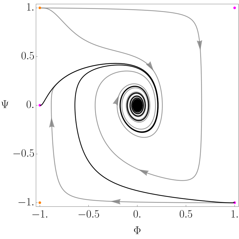
(a) Expansion ($Y>0$).

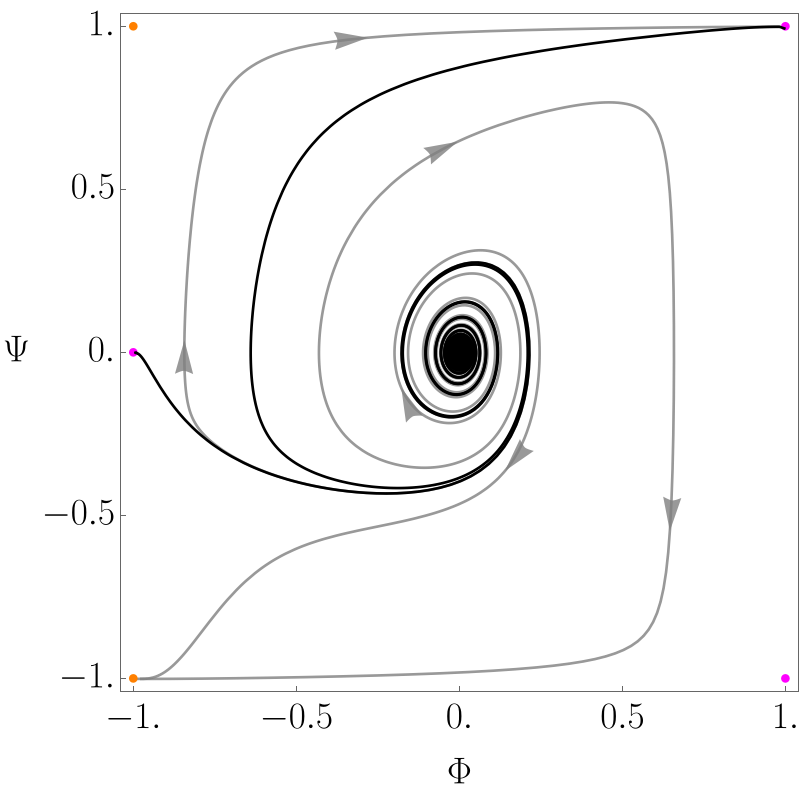
(b) Contraction ($Y<0$).

Figure 1: The flat sub-manifolds for the system, where we substitute $Y>0$ for the expanding case in (a) and $Y<0$ for the contracting case in (b). The Minkowski fixed point is shown in black, the de Sitter fixed points in magenta and the singularities in orange. The two black curves are separatrices that separate where the trajectories expand from (contract to). Trajectories between the two separatrices expand from (contract to) the de Sitter fixed point $dS_{3+}$ ($dS_{2-}$). Otherwise, trajectories outside these separatrices expand from (contract to) $S_{1+}$ ($S_{2-}$).

Going back to the 3-D dynamics, we first consider the $\Phi=-1$ sub-manifold, where the potential (1) reduces to $V=V_{0}$. The fixed points of the $\Phi=-1$ sub-manifold are shown in Table 2, and the phase space is shown in Fig. 2. The Einstein points $E_{\pm}$ are both unstable saddles, with only two separatrix trajectories emerging from each. Therefore, these are not good candidates for emerging models as these are a set of measure zero for the whole phase space. In this sub-manifold, the past repellors for initially expanding models are the singularities $S_{1+}$ and $S_{2+}$, and the de Sitter fixed point $dS_{1-}$ is the past repellor for models which initially contract. Trajectories emerging from the non-singular de Sitter state $dS_{1-}$ either collapse, bounce and expand towards another de Sitter state $dS_{1+}$, or collapse to a singularity ($S_{1-}$ or $S_{2-}$).

Fixed point	$\Psi$	$Y$	Stability in 2-D	Stability in 3-D
$E_{\pm}$	$\pm\frac{1}{\sqrt{2}}$	0	Saddle ($\pm$)	Saddle ($\pm$)
$dS_{1\pm}$	0	$\pm\frac{1}{2}$	Attractor (+)/ Repellor (-)	Saddle ($\pm$)
$dS_{4\pm}$	0	$\pm 1$	Saddle ($\pm$)	Saddle ($\pm$)
$S_{1\pm}$	1	$\pm 1$	Repellor (+)/ Attractor (-)	Repellor (+)/ Saddle (-)
$S_{2\pm}$	-1	$\pm 1$	Repellor (+)/ Attractor (-)	Saddle (+)/ Attractor (-)

Table 2: Fixed points with their stability for the 2-D $\Phi=-1$ sub-manifold in Fig. 2 and the full 3-D phase space in Fig. 3. $E$ denotes the Einstein fixed points, $dS$ the de Sitter fixed points, and $S$ the singularities.

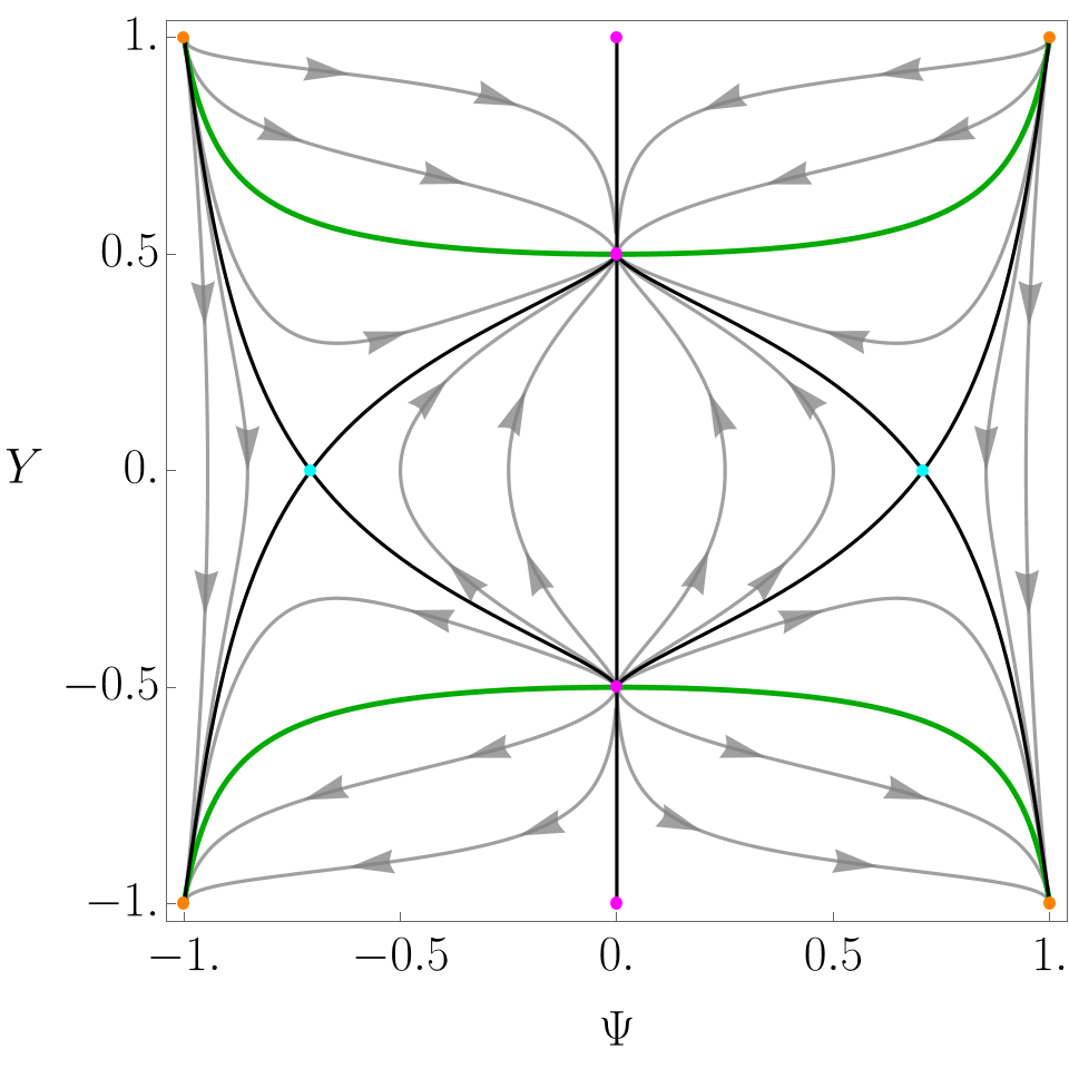
Figure 2: The $\Phi=-1$ submanifold. The thick green curve shows the Flat Friedmann Separatrix (FFS) separating the open models outside the FFS from the closed models between the two green curves. The thick black curve is the Closed Friedmann Separatrix (CFS) which seperates different types of closed models in the phase space. The Einstein fixed points are shown in cyan, the de Sitter fixed points in magenta and the singularities in orange.

The full phase space for the 3-D system is shown in Fig. 3, where Fig. 3(a) shows examples of open (blue) and closed (purple) trajectories coming from and going to a singularity, and Fig. 3(b) shows examples of non-singular trajectories. The fixed points that have not already been considered in the sub-manifolds are shown in Table 3. In Fig. 3(a), there are two examples of closed models: one simply expands from a singularity, reaches a turn-around on the surface $Y=0$ and then collapses to a singularity. The other expands and oscillates around the Minkowski fixed point (at the minimum of the potential), where it contracts, bounces and expands, before turning around on the $Y=0$ surface and collapsing to the singularity. Whether there is a sufficient inflationary phase after the bounce remains to be seen. The expanding open model evolves from a singularity, and oscillates around the minimum of the potential, and the contracting open model oscillates around the Minkowski fixed point before collapsing to a singularity.

Fig. 3(b) shows examples of non-singular models in the phase space, which emerge from Einstein fixed points (cyan) and de Sitter fixed points (magenta). The trajectories that emerge from the Einstein fixed points require extremely fine-tuned initial conditions: they form a set of measure zero in phase space. Trajectories can emerge from the de Sitter states $dS_{4+}$ and $dS_{5+}$, but these are a set of measure zero in the phase space. However, there is a 3-D subset of trajectories emerging from $dS_{3+}$, like the blue trajectory in the figure, but this fixed point is a 3-D saddle, repelling the aforementioned subset and attracting in another sub-manifold. Thus, fine-tuning is still needed to ensure that trajectories emerge from this fixed point. For all other trajectories the past repellor is the $S_{1+}$ point, representing a stiff fluid singularity where the scalar field is kinetic dominated.

Fixed point	$\Phi$	$\Psi$	$Y$	Stability
$dS_{5\pm}$	0	0	$\pm 1$	Saddle ($\pm$)

Table 3: The fixed points of the full system not already shown in the flat and $\Phi=-1$ sub-manifolds.

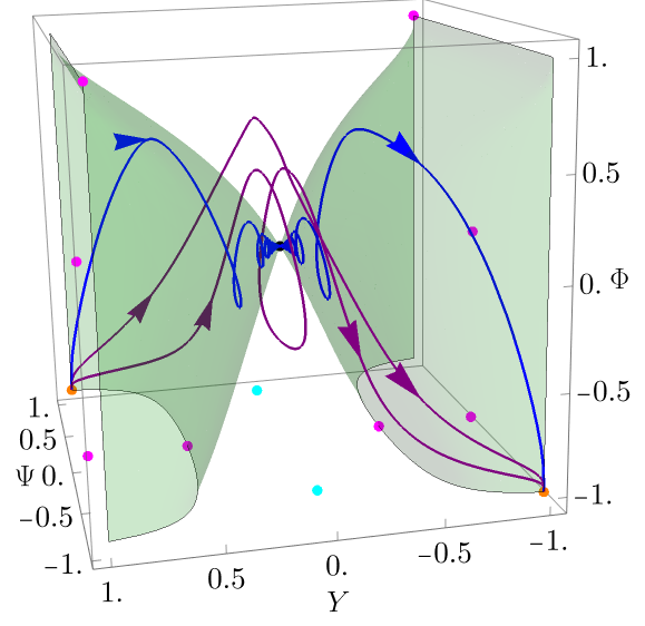
(a) Singular trajectories.

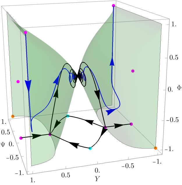
(b) Non-singular trajectories.

Figure 3: The full phase space for the system, where we have plotted examples of open (blue) and closed (purple) trajectories, as well as separatrices (black). The green surface shows the Flat Friedmann Separatrix. The Minkowski fixed point is shown in black, the Einstein fixed points in cyan, the de Sitter fixed points in magenta, and the singularities in orange.

3 Emergence from Interacting Dark Energy and Dark Matter

In this essay, we contend that it is desirable for all trajectories to emerge from a non-singular state in the Emerging Universe scenario, regardless of initial conditions. In the following, we provide an example of a model with dark energy with a non-linear equation of state [25] interacting with a dust fluid [26], where the generic trajectory either represents cyclic models, or models that emerge from an unstable de Sitter phase during expansion. For flat and open models this is the asymptotic past repellor, whilst for a subset of closed models the de Sitter phase represents a transition through a bounce from contraction to expansion.

In this scenario, the conservation equations for the dark matter and dark energy are

$$\dot{\rho}_{m}=-3H\rho_{m}+\frac{H\rho_{x}\rho_{m}}{\rho_{i}}\,,$$ (11)

$$\dot{\rho_{x}}=-3H(\rho_{x}-\rho_{\Lambda})\left(1+w_{x}+\epsilon\frac{\rho_{x}}{\rho_{*}}\right)-\frac{H\rho_{x}\rho_{m}}{\rho_{i}}\,.$$ (12)

where $\rho_{m}$ is the dark matter energy density and $\rho_{x}$ is the dark energy density. The dark energy has a non-linear equation of state, with $w_{x}$ defining its linear part, $\rho_{*}$ the characteristic scale of the non-linear part, and $\rho_{\Lambda}$ representing its low energy attractor. $\epsilon$ is a free dimensionless parameter that fixes the sign and the strength of the quadratic term and the energy scale $\rho_{i}$ characterises the non-linear interaction. To close the system, we also require the Raychaudhuri equation to describe the evolution of the expansion scalar $H$,

$$\dot{H}=-H^{2}-\frac{1}{6}\left[\rho_{m}+\rho_{x}(1+3w_{x}-3\epsilon\frac{\rho_{\Lambda}}{\rho_{*}})\\ -3\rho_{\Lambda}(1+w_{x})+3\epsilon\frac{\rho_{x}^{2}}{\rho_{*}}\right]\,.$$ (13)

To analyse the dynamical system consisting of (11), (12) and (13), we first define dimensionless variables,

$$x=\frac{\rho_{x}}{\rho_{*}},~{}~{}y=\frac{H}{\sqrt{\rho_{*}}},~{}~{}z=\frac{\rho_{m}}{\rho_{*}},~{}~{}\mathcal{R}=\frac{\rho_{\Lambda}}{\rho_{*}},~{}~{}q=\frac{\rho_{*}}{\rho_{i}},~{}~{}\eta=\sqrt{\rho_{*}}t\,,$$ (14)

as well as compactified variables,

$$X=\frac{x}{1+x},~{}~{}Y=\frac{y}{\sqrt{1+y^{2}}},~{}~{}Z=\frac{z}{1+z}\,.$$ (15)

in order to see the behaviour of the system at infinity. For this system, $Y=\pm 1$ corresponds to $H\rightarrow\pm\infty$, and $X=Z=1$ corresponds to $\rho_{x},\rho_{m}\rightarrow+\infty$.

An example of the full phase space for a subset of models that expand towards a future de Sitter state is shown in Fig. 4 with the fixed points shown in Table 4. We set the parameter values to $\epsilon=-0.25$, $q=1$, $\mathcal{R}=0.05$ and $w_{x}=-0.5$, which defines a surface in the phase space. The reddish surface shows where the acceleration is zero, with models accelerating when trajectories are above this surface, and decelerating when they are below it. The Flat Friedmann Separatrix would be a surface in the phase space, however for the sake of clarity we just show the flat trajectories in green for the parameter values we set. There is a trajectory, not shown in the figure, which connects the flat fixed points $dS_{3+}$ and $dS_{3-}$. This is a high energy de Sitter trajectory, representing a closed de Sitter model.

In this case, all trajectories are non-singular and emerge from either a de Sitter or Einstein fixed point. Open (blue) and flat models emerge from a de Sitter fixed point (magenta) and expand (contract) to another de Sitter state. The Closed Friedmann Separatrix (CFS) passing through the saddle Einstein point is shown by the thick black curve. Closed models (purple) outside the CFS emerge from a contracting phase asymptotic in the past to the de Sitter fixed point $dS_{1-}$, then bounce at high energy before expanding to $dS_{1+}$. Trajectories inside the CFS either bounce once, contracting from $dS_{1-}$ and expanding to $dS_{1+}$, or are cyclic around the Einstein fixed point $E_{2}$, and repeatedly contract, bounce and expand. An emergent case which expands from the Einstein fixed point $E_{1}$ also exists along the CFS.

In this example, two Einstein fixed points (cyan) exist in the phase space, which coincide with where the acceleration is zero. This means in this example, open, flat and closed trajectories outside of the CFS all evolve with an early- and late-time acceleration, connected by a decelerated period. These are the cases of interest as they qualitatively match the observed Universe.

Fixed point	$X$	$Y$	$Z$	Stability
$dS_{1\pm}$	0.048	$\pm$0.13	0	Attractor (+)/ Repellor (-)
$dS_{2\pm}$	0.67	$\pm$ 0.63	0	Saddle ($\pm$)
$dS_{3\pm}$	0.75	$\pm$ 0.74	0.42	Spiral saddle ($\pm$)
$dS_{4\pm}$	0.75	$\pm$ 1	0.42	Spiral repellor (+)/ Spiral attractor (-)
$E_{1}$	0.052	0	0.094	Saddle
$E_{2}$	0.73	0	0.87	Centre

Table 4: Fixed points for the fluid model, where dust is interacting with a dark energy with a non-linear equation of state. The parameters are set to $\epsilon=-0.25$, $q=1$, $\mathcal{R}=0.05$ and $w_{x}=-0.5$.

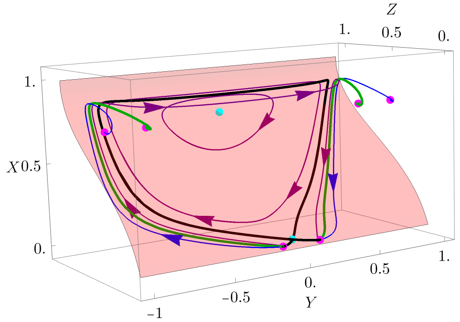
(a)

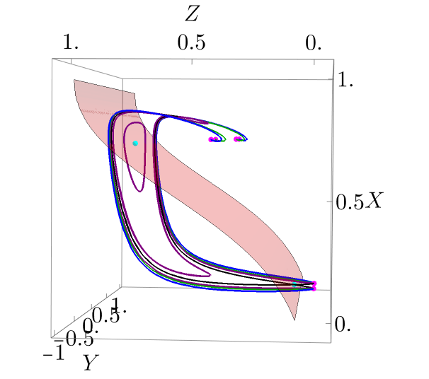
(b)

Figure 4: The full phase space for the interacting cold dark matter and dark energy model, where the parameters are set to $\epsilon=-0.25$, $q=1$, $\mathcal{R}=0.05$ and $w_{x}=-0.5$. The reddish surface shows where the acceleration is zero, with trajectories accelerating above this surface and decelerating below it. The green trajectories show the flat models and the black curves show the Closed Friedmann Separatrix (CFS). Open models are shown in blue, and closed models are shown in purple. All trajectories are non-singular, emerging from either an Einstein fixed point (cyan) or a de Sitter fixed point (magenta). We only show the fixed points that are relevant to the dynamics; the full list of fixed points can be seen in Table 4.

4 Conclusions

In this essay, we have carried out a dynamic systems analysis of the Emergent Universe scenario in [1], which consists of a scalar field with an asymmetric potential with a plateau for negative $\phi$. Originally, this scenario was considered with specific initial conditions such that the universe emerged from a static Einstein state. The aim of this essay was to understand whether the past repellor was generically non-singular for any initial conditions. The de Sitter model is normally associated to a cosmological constant associated with an asymptotically stable future attractor [27, 28], but it can also represent a past repelling fixed point [29, 25]. We found a class of models which emerged from a non-singular de Sitter fixed point, however the stability of this point is that of a 3-D saddle, so some level of fine-tuning is required. All other trajectories expand from a singularity. We remark that simply with the exchange $\phi\rightarrow-\phi$ the potential (1) for the model in [1] becomes the potential for the Einstein-frame version [30] of Starobinsky inflation [31], hence our analysis can easily be mapped into one for that model. Models of this type are currently the most favored by experimental results [32, 33].

With the aim of showing a scenario where emergence from a non-singular state is generic during expansion, we then considered a fluid model with interacting dark energy and dark matter. In this case, it is not necessary to have a quantum gravity era at high energy to avoid a singularity. Instead we have a classical de Sitter vacuum-dominated era at high energy from which our models emerge from, which is a past attractor for flat and open models, or a transition phase through a bounce for a subset of closed models. We also highlighted the models of interest that evolve with an early- and late-time acceleration connected by a decelerated period, which include open, flat and closed models. Therefore, at least qualitatively, these models are consistent with the observable Universe and emerge from a non-singular de Sitter state.

For FLRW models that have a singularity, it is well known that this is very special in that it is matter dominated, while in more general GR models the shear anisotropy becomes dominant in approaching the singularity, which is said to be velocity dominated, e.g. see [34] and refs. therein. More in general, especially for bouncing models with a contracting phase, the question is if the singularity avoidance found in the FLRW case is stable against shear anisotropy [35]. In a long-wavelength approximation to inhomogeneities [36], this question can be investigated by generalising non-singular FLRW models with a bounce to anisotropic Bianchi IX models, see [37] and refs. therein. This will be the goal of our future investigation, generalising the non-singular scenario presented here based on dark matter interacting with dark energy, to study the stability of the results [26].

References

- [1] G. F. R. Ellis and R. Maartens. The emergent universe: Inflationary cosmology with no singularity. Class. Quant. Grav., 21:223–232, 2003.
- [2] P. Joshi. Global Aspects in Gravitation and Cosmology. Oxford University Press Inc., 1993.
- [3] S. Hawking and W. Israel. General Relativity: An Einstein Centenary Survey. Cambridge University Press, 1979.
- [4] G. W. Gibbons, E. P. S. Shellard, and S. J. Ranking, editors. The Future of Theoretical Physics and Cosmology. Cambridge University Press, 2003.
- [5] A. Ashtekar, B. K. Berger, J. Isenberg, and M. MacCallum, editors. General Relativity and Gravitation: A Centennial Perspective. Cambridge University Press, 2015.
- [6] N. Aghanim, Y. Akrami, F. Arroja, M. Ashdown, et al. Planck 2018 results. I. Overview and the cosmological legacy of Planck. Astronomy & Astrophysics, 641, 2020.
- [7] N Aghanim, Y. Akrami, M. Ashdown, J. Aumont, et al. Planck 2018 results. VI. Cosmological parameters. Astronomy & Astrophysics, 641, 2020.
- [8] E. Di Valentino et al. Snowmass2021 - Letter of interest cosmology intertwined IV: The age of the universe and its curvature. Astropart. Phys., 131:102607, 2021.
- [9] G. F. R. Ellis, K. A. Meissner, and H. Nicolai. The physics of infinity. Nature Physics, 14:770–772, 8 2018.
- [10] G. F. R. Ellis, J. Murugan, and C. G. Tsagas. The emergent universe: An explicit construction. Classical and Quantum Gravity, 21:233–249, 1 2004.
- [11] S. Mukherjee, B. C. Paul, N. K. Dadhich, S. D. Maharaj, and A. Beesham. Emergent universe with exotic matter, 2006.
- [12] E. Verlinde. Emergent gravity and the dark universe. SciPost Physics, 2, 6 2017.
- [13] G. F. R. Ellis, E. Platts, D. Sloan, and A. Weltman. Current observations with a decaying cosmological constant allow for chaotic cyclic cosmology. Journal of Cosmology and Astroparticle Physics, 2016, 4 2016.
- [14] L. Parisi, M. Bruni, R. Maartens, and K. Vandersloot. The Einstein static universe in Loop Quantum Cosmology. Class. Quant. Grav., 24:6243–6253, 6 2007.
- [15] D. J. Mulryne, R. Tavakol, J. E. Lidsey, and G. F. R. Ellis. An emergent universe from a loop. Phys. Rev. D, 71:123512, 2005.
- [16] A. Bonanno, G. Gionti, and A. Platania. Bouncing and emergent cosmologies from ADM RG flows. Class. Quant. Grav., 35, 2017.
- [17] G. Gionti. Hamiltonian Analysis of Asymptotically Safe Gravity. PoS, CORFU 2017:192, 2017.
- [18] R. Sengupta. A novel model of non-singular oscillating cosmology on flat Randall-Sundrum II braneworld. 2023.
- [19] J. D. Barrow, G. F. R. Ellis, R. Maartens, and C. G. Tsagas. On the Stability of the Einstein Static Universe. Class. Quant. Grav., 20:155–164, 2003.
- [20] A. S. Eddington. On the instability of Einstein’s spherical world. MNRAS, 90:668–678, 1930.
- [21] L. Amendola, M. Litterio, and F. Occhionero. The phase-space view of inflation: I. the non-minimally coupled scalar field. International Journal of Modern Physics A, 5:3861–3886, 1990.
- [22] V. A. Belinskii, L. P. Grishchuk, Ya. B. Zel’dovich, and I. M. Khalatniko. Inflationary stages in cosmological models with a scalar field. Sov. Phys. JETP, 62:195, 1985.
- [23] D. K. Arrowsmith and C. M. Place. Ordinary Differential Equations. Chapman and Hall, 1982.
- [24] D. K. Arrowsmith and C. M. Place. Dynamical systems: differential equations, maps and chaotic behaviour. Chapman and Hall, 1992.
- [25] M. Burkmar and M. Bruni. Bouncing cosmology from nonlinear dark energy with two cosmological constants. Phys. Rev. D, 107:083533, 4 2023.
- [26] M. Burkmar and M. Bruni. In preperation, 2024.
- [27] Robert M. Wald. Asymptotic behavior of homogeneous cosmological models in the presence of a positive cosmological constant. Phys. Rev. D, 28:2118–2120, 1983.
- [28] Marco Bruni, Filipe C. Mena, and Reza K. Tavakol. Cosmic no hair: Nonlinear asymptotic stability of de Sitter universe. Class. Quant. Grav., 19:L23–L29, 2002.
- [29] Kishore N. Ananda and Marco Bruni. Cosmological dynamics and dark energy with a nonlinear equation of state: A quadratic model. Phys. Rev. D, 74:023523, 2006.
- [30] K. Maeda. Inflation as a transient attractor in cosmology. Phys. Rev. D, 37:858–862, Feb 1988.
- [31] A. A. Starobinsky. A New Type of Isotropic Cosmological Models Without Singularity. Phys. Lett. B, 91:99–102, 1980.
- [32] Y. Akrami, F. Arroja, M. Ashdown, J. Aumont, et al. Planck 2018 results: X. Constraints on inflation. Astronomy & Astrophysics, 641, 2020.
- [33] A. Kehagias, A. M. Dizgah, and A. Riotto. Remarks on the Starobinsky model of inflation and its descendants. Phys. Rev. D, 89(4):043527, 2014.
- [34] J. Wainwright and G. F. R. Ellis. Dynamical Systems in Cosmology. Cambridge University Press, 1997.
- [35] V. Bozza and M. Bruni. A Solution to the anisotropy problem in bouncing cosmologies. JCAP, 10:014, 2009.
- [36] L. D. Landau and E. M. Lifshitz. The Classical Theory of Fields, volume 2 of Course of Theoretical Physics. Pergamon Press, Oxford, 1975.
- [37] C. Ganguly and M. Bruni. Quasi-isotropic cycles and non-singular bounces in a mixmaster cosmology. Phys. Rev. Lett., 123:201301, 2 2019.