Atomic momentum distributions in polyatomic molecules in rotational-vibrational eigenstates
Abstract
We report a quantum mechanical method for calculating the momentum distributions of constituent atoms of polyatomic molecules in rotational-vibrational eigenstates. Application of the present theory to triatomic molecules in the rovibrational ground state revealed that oscillatory changes appear on the proton momentum distribution in the nonlinear \ceH2O molecule, whilst no such modulation is present in the case of an oxygen atom in the linear \ceCO2 molecule. The atomic momentum distributions were analyzed in detail by means of a rigid rotor model, and it was found that the oscillation originates from quantum-mechanical delocalization of the target atom with respect to the other atoms.
I Introduction
Nuclear quantum effects (NQEs), such as zero-point energy and tunneling, play a crucial role in numerous phenomena of importance in materials science, chemistry, and biology, e.g., static and dynamical properties of hydrogen bonding systems, proton transfer reactions, and diffusion in bulk and confined environments.Ceriotti et al. (2016); Tuckerman and Ceperley (2018); Fang et al. (2019) Deep Inelastic Neutron Scattering (DINS)Evans et al. (1993); Watson (1996); Mayers et al. (2002); Andreani et al. (2005, 2017) has attracted recently considerable interest, because it provides information on momentum distribution of constituent atoms in matter, which is sensitive to the NQEs. For example, DINS experiments have revealed a striking bimodal profile of the proton momentum distribution in KDP,Reiter et al. (2002) confined water in nanomaterials,Reiter et al. (2012); Garbuio et al. (2007) and hydrated water in proteins.Senesi et al. (2007) The bimodal shape was regarded as a result of the proton tunneling, or coherent delocalization of the proton over different sites.Reiter et al. (2004); Garbuio et al. (2007) Furthermore, the oscillatory behavior of the atomic momentum distribution has been also reported for a tunneling phenomenon with respect to rotational motion of water in beryl.Kolesnikov et al. (2016)
Many of the DINS experimental results, including the bimodal distribution described above, were interpreted by means of an effective single-particle model, where atomic momentum distributions is evaluated under approximation with single-particle motion in an effective (Born-Oppenheimer) mean field potential.Reiter et al. (2002, 2004, 2012); Senesi et al. (2007); Garbuio et al. (2007); Reiter and Silver (1985); Andreani et al. (2001); Homouz et al. (2007); Flammini et al. (2012) However, it remains uncertain whether or not the correlated motions in quantum many-body systems can be reduced to the single-particle motions, and the interpretation of the DINS experimental results based on the single-particle model is subject to some controversy.Soper (2009); Lin et al. (2011); Wu and Car (2020) In order to elucidate the physics behind the atomic momentum distribution, an associated quantum calculation that treats all degrees of freedom of nuclei are of crucial importance.
Path integral molecular dynamics (PIMD) is the state-of-the-art method for calculating atomic momentum distributions in molecular systems.Lin et al. (2011); Wu and Car (2020); Morrone and Car (2008); Lin et al. (2010); Ceriotti and Manolopoulos (2012) Using PIMD, ensemble averages of atomic momentum distributions can be calculated under explicit consideration of quantum behavior of nuclei (except for particle exchange) in many-body systems. Although PIMD results can be compared directly to experimental results, it is difficult to capture individual contributions from an each single quantum state, since they are smeared out by the ensemble average.Wu and Car (2020) To investigate such NQEs at the most fundamental level, it is essential to develop a new theory suitable to a single quantum state of isolated molecules, whose wavefunctions are usually well characterized.
For diatomic molecules in their rotational-vibrational eigenstates, such a quantum theory for the atomic momentum distribution has already been well established.Colognesi and Pace (1999); Andreani et al. (1995); Tachibana et al. (2022) Colognesi et al. revealed that the atomic momentum distribution exhibits a clear oscillation originating from the quantum-mechanical rotation, of which wavelength is related to the internuclear distance.Colognesi and Pace (1999) To discuss the generality of this oscillation for three-atom or larger systems, it is highly expected to extend the quantum treatment from diatomic molecules to any kind of polyatomic molecules.
At present, however, the quantum effects on atomic momentum distributions in polyatomic molecules remains still to be investigated. Colognesi et al. have proposed a quantum treatment based on the position autocorrelation function, but the target is restricted to symmetric top molecules.Colognesi et al. (2001) They calculated the proton momentum distribution of the ground state \ceNH3 but did not investigate any quantum effect, by simply concluding that molecular rotations can be dealt with classically at higher temperature. Thus, issue still remains; whether or not the quantum oscillation is also present in the atomic momentum distribution in any kind of molecules other than diatomics; if it presents, what is the origin of it?
In this study, we report a quantum treatment for calculating the atomic momentum distribution in polyatomic molecules in rotational-vibrational eigenstates. Different from the previous method based on the autocorrelation function,Colognesi et al. (2001) our approach utilizes momentum-space molecular wavefunctions themselves, which is a significant extension of the quantum treatment for diatomic moleculesColognesi and Pace (1999) to polyatomic molecules having arbitrary symmetry. A practical example of triatomic molecules (\ceH2O and \ceCO2) in its rovibrational ground state has clearly shown a distinct oscillation appeared in the proton momentum distribution in the nonlinear \ceH2O molecule but not in the case of an oxygen atom in the linear \ceCO2 molecule. The origin of the oscillatory structure and the difference in the results between \ceH2O and \ceCO2 are discussed in terms of the quantum-mechanical distribution of the target atom with respect to the other constituent atoms, which is determined by the rotational-vibrational wavefunction.
II Theory
II.1 Atomic momentum distributions obtained through momentum-space molecular wavefunctions
The momentum distribution of the th atom in an N-atomic molecule in a single quantum state is defined by
| (1) |
where is the momentum of the th atom, and is the momentum-space molecular (translational, rotational, and vibrational) wavefunction in the Cartesian coordinate system with the position of the th atom. Since the momentum and position operators satisfy the canonical commutation relation, is obtained by the Fourier transform of the position-space wavefunction in the Cartesian coordinate system ,
| (2) |
However, in the rotational-vibrational eigenstate, the position-space wavefunction is usually expressed as in the generalized coordinate system , where are the center-of-mass coordinates, are the Euler angles, and are the normal coordinates.Wilson et al. (1955); Bunker and Jensen (2006) For nonlinear molecules, and ; for linear molecules, and .
Hence, to calculate of Eq. 2, the change of variables from to is necessary. According to the Podolsky trick,Podolsky (1928); Wilson et al. (1955); Bunker and Jensen (2006) which is used in the derivation of the rotational-vibrational Hamiltonian for , the is related to the by
| (3) |
where is the position-space wavefunction in the mass-weighted coordinate system with the mass of the th atom. and are the determinant of the matrices and whose components are expressed as
| (4a) | |||
| (4b) | |||
The volume elements in the coordinates , , and are connected by and as follows:
| (5) |
with and . Eq. 3 was originally introduced by Podolsky to satisfy Eq. 5 and the normalization condition of the wavefunctions , , and ,
| (6) |
| (7) |
where is the Jacobian of with respect to .
II.1.1 Separation of translational and internal motions
In the absence of external fields, the position-space wavefunction is written as the product of the translational and rotational-vibrational wavefunctions :Wilson et al. (1955); Bunker and Jensen (2006)
| (8) |
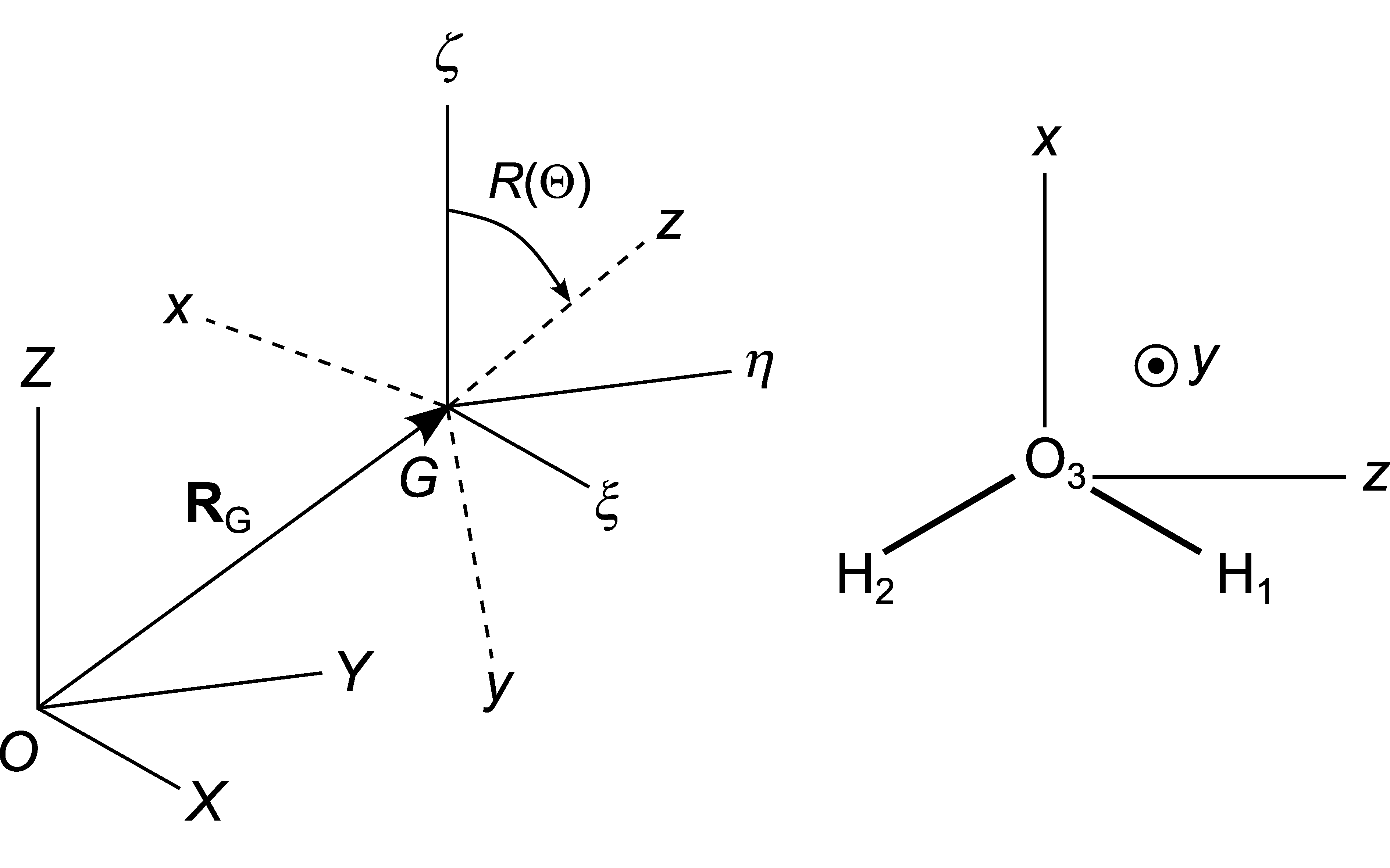
Also, can be separated into the two parts by setting the coordinate frames as shown in Fig. 1, as follows. Here the center-of-mass frame is moved by from the space-fixed frame , and the molecule-fixed frame is converted from the frame by the rotation matrix . Then, the coordinates of the th atom in the space-fixed frame are expressed as
| (9) |
with being the coordinates in the frame. From the definition of the center-of-mass coordinates,
| (10a) | |||
| (10b) | |||
where is the total mass of the molecule. On the other hand, the momentum of the th atom is expressed as
| (11) |
in terms of the total momentum and the momentum of the th atom in the center-of-mass frame, which satisfy
| (12a) | |||
| (12b) | |||
Using Eqs. 9, 10, 11 and 12, we can write the phase of the plane wave in Eq. 7 as
| (13) |
Substituting Eqs. 8 and 13 into Eq. 7, we obtain
| (14) |
where
| (15) | |||
| (16) |
In the derivation of Eq. 14, we have made use of the fact that is independent of , as shown in the Appendix A.
From Eqs. 12 and 14, we can rewrite the atomic momentum distribution as
| (17) |
where and
| (18) |
with and the momentum space which satisfies . Eq. 17 means that we can calculate by the convolution of the atomic momentum distribution due to the internal (rotational and vibrational) motion and the translational momentum distribution . The energy eigenstates of translational motion in free molecular systems are momentum eigenstates, and hence it is not necessary to consider the translational contribution as long as stationary states are considered. Hereafter, we will focus only on the internal motion by setting so that the atomic momentum distribution is expressed as
| (19) |
II.1.2 The coordinates in the center-of-mass frame and the Jacobian expressed by the generalized coordinates
To obtain for a given , we have to evaluate the integral in Eq. 18 using of Eq. 16. In this case, it is necessary to express both the coordinates in the center-of-mass frame and the Jacobian as functions of the generalized coordinates.
Since the molecule-fixed frame is converted from the center-of-mass frame by the rotation matrix as shown in Fig. 1, the coordinates in the frame and satisfy the following relationship:
| (20) |
where we treat and as column vectors. In the Z-Y-Z convention of the Euler angles, is expressed as
| (21) |
where c and s represent cosine and sine, respectively. For linear molecules, is an arbitrary function of ,Watson (1970) and we set . According to the theory of molecular vibration, we can separate into the equilibrium coordinates and the displacements which are further decomposed into normal modes:Wilson et al. (1955)
| (22a) | |||
| (22b) | |||
with the vibrational degrees of freedom . The expansion coefficients satisfy the orthogonality and the Eckart conditions:Watson (1968); Eckart (1935)
| (23a) | |||
| (23b) | |||
| (23c) | |||
Using Eqs. 20 and 22, we can rewrite as
| (24) |
which enables us to calculate the Jacobian . After some mathematical transformations (see Appendix A), we obtain
| (25) |
The general form of for nonlinear molecules is given by
| (26) |
where is the component of the effective inertia tensor (with respect to the molecule-fixed frame) defined byWatson (1968)
| (27) |
with
| (28) | |||
| (29) |
is the instantaneous inertia tensor, and is the Coriolis coupling coefficient. For linear molecules, is written as
| (30) |
The effective moment of inertia is related to as follows:Watson (1970); Amat and Henry (1958)
| (31a) | |||
| (31b) | |||
where the -axis is the molecular axis of linear molecules.
II.2 Rigid-rotor-harmonic-oscillator approximation
Since and are obtained as the functions of , we can calculate by using Eq. 16. However, to obtain , the -dimensional integral must be performed for each point of in the momentum space. In order to reduce the computational cost, we introduce the rigid-rotor-harmonic-oscillator (RRHO) approximation.
Using Eq. 24, we can write the phase of plane wave in Eq. 16 as
| (32) |
where
| (33a) | |||
| (33b) | |||
Substituting Eqs. 32 and 25 into Eq. 16, we rewrite
| (34) |
with being the rotational degrees of freedom. The integration with respect to in Eq. 34 is regarded as the Fourier transform of . By applying the RRHO approximation to and , we will calculate this Fourier transform analytically.
In the RRHO approximation, is separated into the rigid rotor and harmonic oscillator wavefunctions:Wilson et al. (1955); Bunker and Jensen (2006)
| (35) |
The normalization conditions of and are given by
| (36) |
with . is expressed as the product of the harmonic oscillator wavefunctions for each normal mode of the molecule:
| (37) |
with
| (38) |
where is the vibrational quantum number, is the angular frequency, and is the th-order Hermite polynomial. In the rigid rotor approximation of , we write
| (39) |
This treatment is equivalent to used in the RRHO approximation of the rotation-vibration Hamiltonian.Wilson et al. (1955); Bunker and Jensen (2006) Substituting Eqs. 35 and 39 into Eq. 34, we obtain
| (40) |
with . is the Fourier transform of and is written as
| (41) |
where
| (42) |
Finally, we can calculate the atomic momentum distribution within the RRHO framework by using Eqs. 18, 19 and 40.
III Computational details
To investigate the quantum effects on the atomic momentum distribution, the calculations of atomic momentum distributions were performed within the two kinds of frameworks, i.e., the quantum and semiclassical ones, dealing with molecular free rotations in quantum and classical ways, respectively. In both cases, we set and utilize the RRHO approximation. The target are nonlinear and linear triatomic molecules, \ceH2O and \ceCO2, in their rotational-vibrational ground state ().
III.1 Quantum framework
In the rotational-vibrational ground state (the angular momentum quantum number and ), the rotational wavefunction of nonlinear (or linear) molecules is given by
| (43) |
Putting Eq. 43 into Eq. 40, it is evident that has the following rotational symmetry:
| (44) |
Therefore, the atomic momentum distribution of Eq. 18 becomes isotropic in the space-fixed frame:
| (45) |
From Eqs. 17, 19, 45 and 18, the atomic momentum distribution of the target atom A in a triatomic molecule (ABC) can be written as
| (46) |
| where we replace with . Since the atomic momentum distribution in the ground state is isotropic, we just consider one-dimensional distribution for and express by using the cylindrical coordinates, | |||
| (47a) | |||
| (47b) | |||
Using Eq. 44 with rotations around the -axis, has cylindrical symmetry about :
| (48) |
Therefore, we can rewrite Eq. 46 as
| (49) |
with .
In order to calculate the physical quantities for \ceH2O and \ceCO2 were calculated at the HF/6-31G(d,p) level using the Gaussian16 program.Frisch et al. (2016) In determining and , we set the axes of the molecule-fixed frame as with the principal axes at the equilibrium molecular structure, where the principal moments of inertia satisfy . For \ceCO2, the axis coincides with the molecular axis, i.e., the axis.
In the numerical evaluation of Eq. 40, the integrand is periodic for and , but not for . Therefore, we used the trapezoidal integration for and , and the tanh-sinh quadrature for with
| (50) |
where we set . For \ceH2O, the numbers of sampled points are 100, 200, and 100 for , , and , respectively; for \ceCO2, 100 and 400 for and , respectively.
| Molecule(Atom A,B) | ||||
|---|---|---|---|---|
| \ceH2O(\ceH1,\ceH2) | 0.1 | 0–20 | 0–15 | –15 |
| \ceCO2(\ceO1,\ceO2) | 0.1 | 0–40 | 0–15 | –30 |
From obtained in the way described above, we calculated of Eq. 49 by using the trapezoidal integration. The step size and the ranges of the momentum , , and are shown in Table 1. To evaluate the accuracy of these integration, we calculated the squared norm and the average kinetic energy , which are obtained in the case of isotropic momentum distribution as
| (51) | |||
| (52) |
III.2 Semiclassical framework
IV Results and Discussion
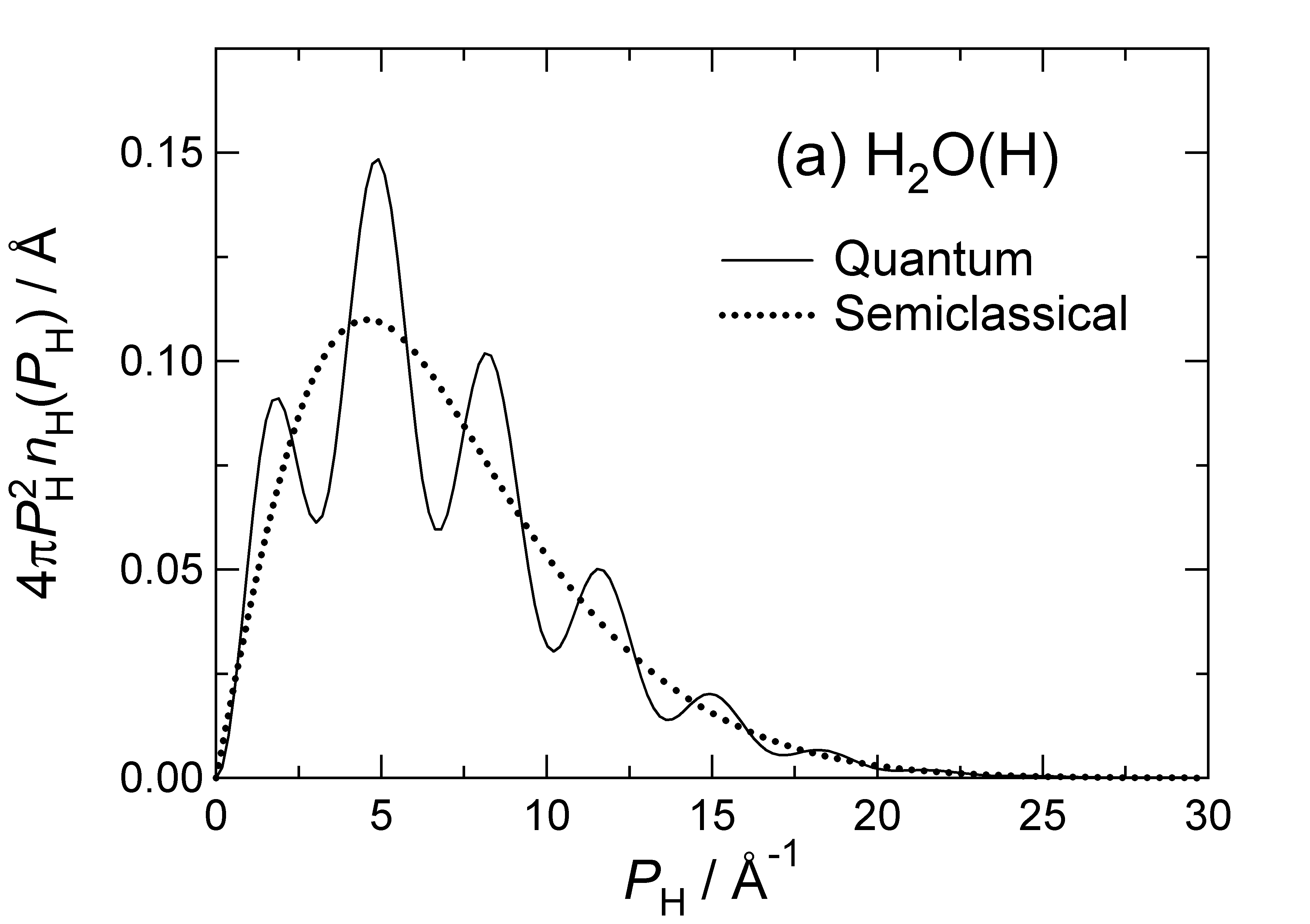
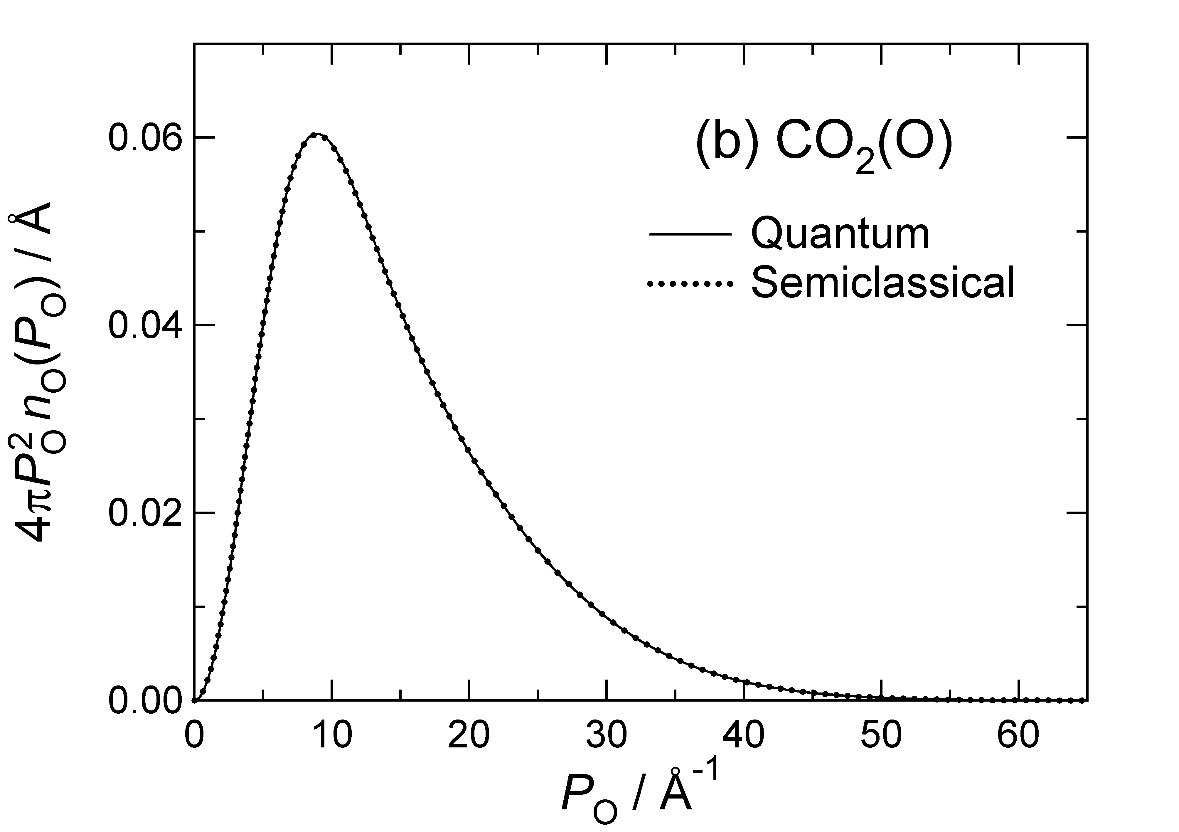
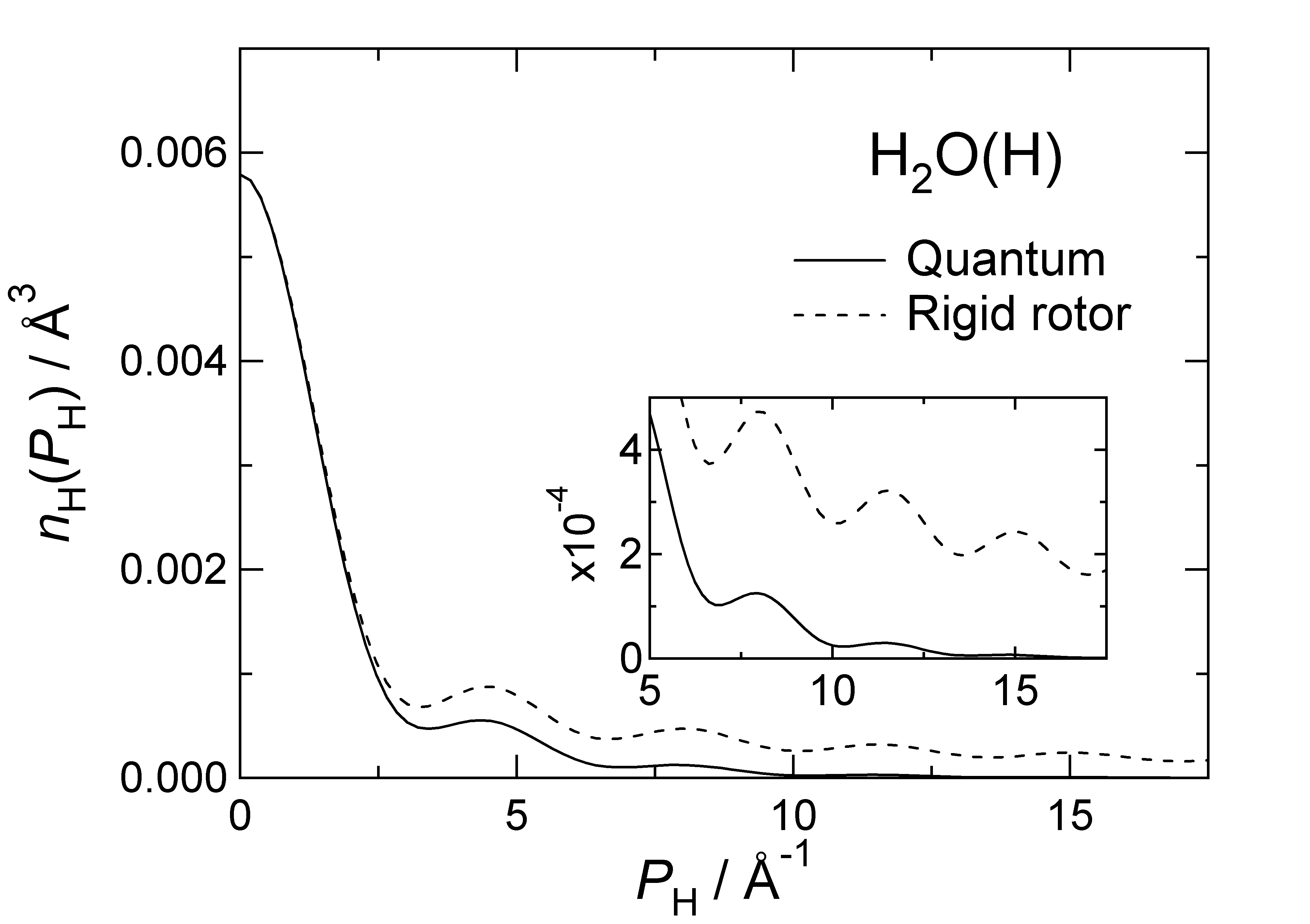
Fig. 2 shows the calculated momentum distributions of the \ceH1 atom in \ceH2O and those of the \ceO1 atom in \ceCO2, which were multiplied by a factor of in order to highlight structures appeared in the distributions. The calculated values for the squared norm are listed in Table 2. They are almost unity, which demonstrates the validity of the RRHO approximation. In addition, the values calculated by the quantum treatment with Eq. 52 are in reasonable agreement with the theoretical values estimated by the semiclassical treatment with Eq. 54. From Fig. 2, it is evident that an oscillatory structure appears in the H-atom momentum distribution in \ceH2O calculated within the framework of the quantum theory. On average, the result of the quantum calculation is in good agreement with that of the semiclassical calculation. On the other hand, no oscillatory behavior is found in the quantum result for the O-atom momentum distribution in \ceCO2.
| Target Atom in Molecule | ||||
|---|---|---|---|---|
| Calc. | Theo. | Calc. | Theo. | |
| \ceH in H2O | 1.03 | 1 | 132 | 134 |
| \ceO in CO2 | 0.99 | 1 | 37.1 | 36.8 |
The oscillation in the quantum momentum distribution for \ceH2O(H) can be understood qualitatively as follows. Substituting Eq. 2 into Eq. 1, we can rewrite as
| (56) |
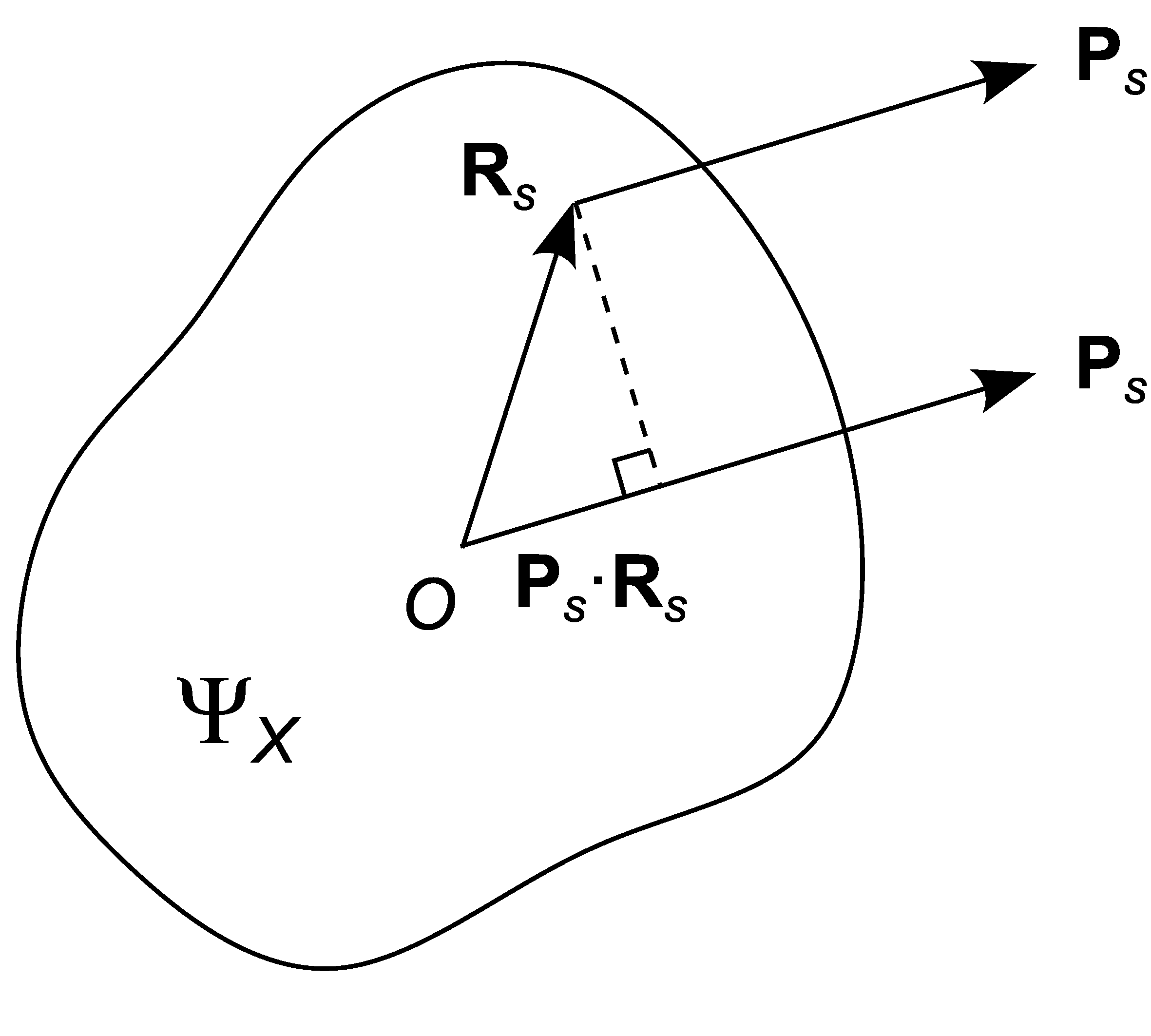
By analogy with the atomic scattering factor,Cullity and Stock (2001); Waseda et al. (2011) the Fourier transform in Eq. 56 can be considered as a superposition of plane waves emitted from all positions with amplitude and wave vector , which is illustrated in Fig. 3. Then, the momentum distribution of the target atom corresponds to the intensity of the resultant wave averaged over all spatial configurations of the other atoms .
The amplitude of the plane wave, defined in the Cartesian coordinate system, is separated into translational and rotational-vibrational parts, as was the case for the generalized coordinate system:
| (57) |
where is identical to , and is regarded as a function on the whole position space, satisfying
| (58) |
Since we assumed , can be expressed as the wavefunction of a free particle in its ground state:
| (59) |
where is the volume of the space . Therefore, is independent of and is determined only by the rotatinal-vibrational part .
In the vibrational ground state, has an amplitude only near equilibrium atomic configurations of the target molecule. If we treat the molecule as a perfect rigid rotor, only the orientational average () of needs to be considered in order to take into account the spatial average of in Eq. 56. As a result of this rigid rotor model, the atomic momentum distribution can be expressed as
| (60) |
Here the region indicates not only the initial configuration but also the other configurations of that coincide with the equilibrium structure. The presence of the thus means that the target atom is spatially delocalized, resulting in interference of the plane waves emitted from them.
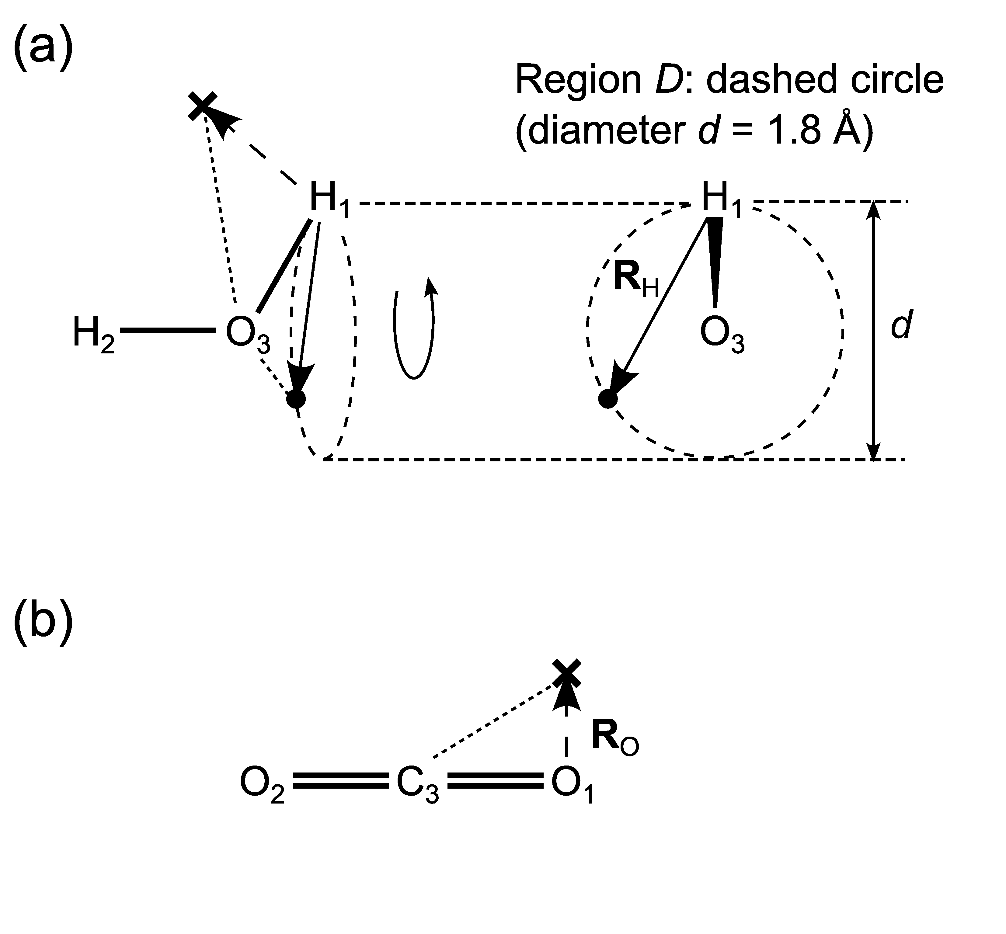
Fig. 4 illustrates the interference effect on the in terms of the spatial delocalization of the target atom. The Fourier integral in Eq. 56 is carried out with respect to the , while keeping the other atoms fixed at a configuration . For the region where , the integrand is vanishingly small. In the case of \ceH2O, thereby, \ceH1 configuration which leads to significantly deformed structures from the equilibrium one [e.g., a configuration marked by cross in Fig. 4(a)] have no contribution to the Fourier transform in Eq. 56. However, the \ceH1 configurations which are identical to those obtained by the rotation with respect to the \ceH2-O3 axis can have some contributions to the integral. The dashed circle drawn in Fig. 4(a) indicates such possible configurations of \ceH1, which corresponds to the region specified in Eq. 60 for the rigid rotor model. Quantum mechanically, this situation represents rotational delocalization of the target \ceH1 atom with respect to the \ceH2 and \ceO3 atoms. Therefore, the plane waves emitted from the different positions of the \ceH1 interfere constructively or destructively each other depending on the momentum of the \ceH1, which results in the oscillation in the proton momentum distribution. This kind of interference can occur in \ceH2O because of the nonlinear molecular structure. For the linear triatomic molecule, \ceCO2, such interference is impossible since the \ceO1 atom is localized with respect to the \ceO2 and \ceC3 atoms, and hence no oscillation due to the quantum interference appears in the O atom’s momentum distribution in \ceCO2.
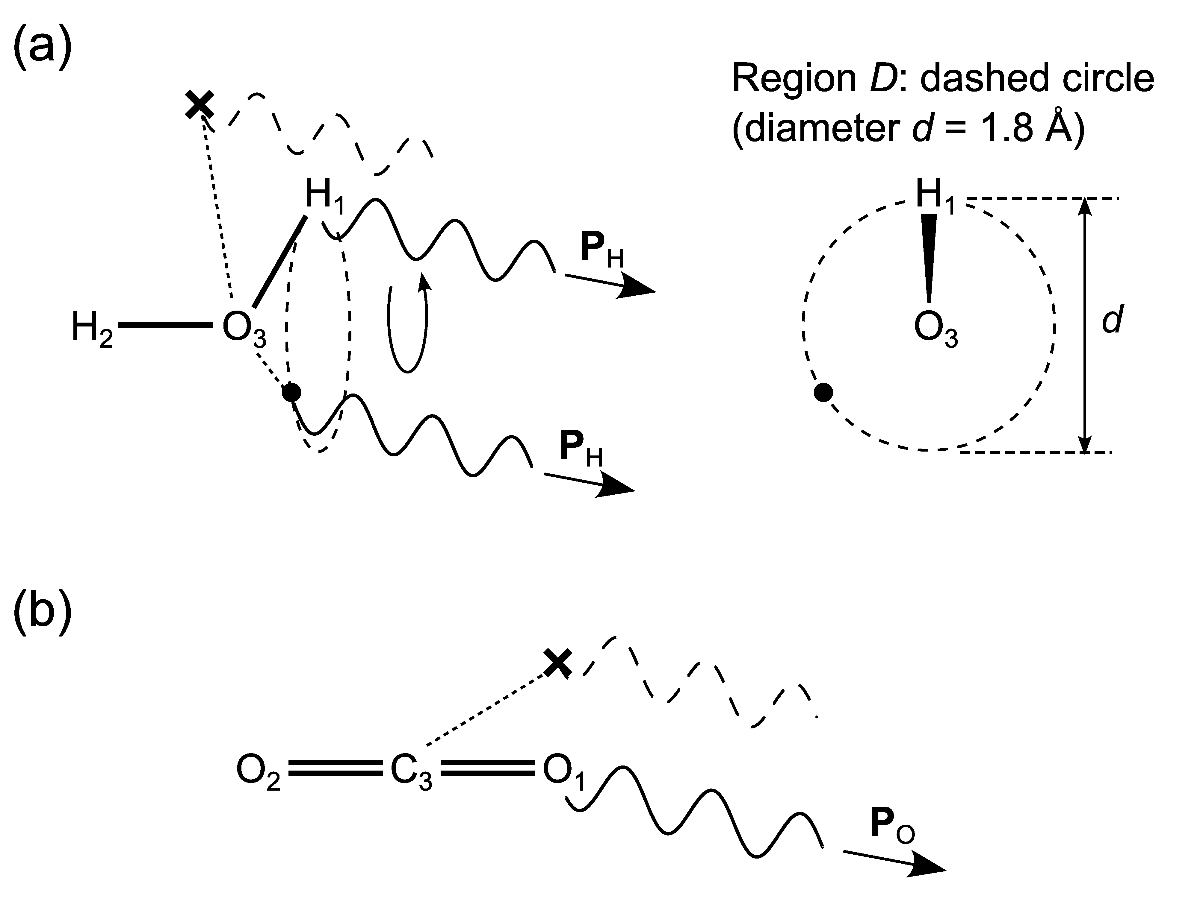
To demonstrate the validity of the above interpretation, we performed the calculation of Eq. 60 for \ceH2O(H) using the rigid rotor model. The region of integration is set to be just a circumference with a diameter as shown in Fig. 4, which is formed by the trajectory of the target \ceH1 atom rotating with respect to the \ceH2-O3 axis by keeping the equilibrium structure of \ceH2O. In addition, is just a constant on the for the rotational ground state. Using these simplifications, we can rewrite Eq. 60 as
| (61) |
where is the zeroth-order Bessel function of the first kind. Fig. 5 compares the rigid rotor model calculation of Eq. 61 with the quantum calculation obtained from Eq. 49. It is evident from the figure that the period of the oscillation is well reproduced by the restricted rigid rotor model though the intensity is overestimated. Therefore, it is concluded that the essential feature of the oscillation is originated from the quantum interference due to the rotational delocalization of the target atom.
An alternative way of interpreting the oscillation in the quantum momentum distribution for \ceH2O(H) can be provided by the autocorrelation of the position-space wavefunction,
| (62) |
which can be obtained by the inverse Fourier transform of the atomic momentum distribution,
| (63) |
Since we consider here only the rotational ground state, is isotropic. Using the expansion of a plane wave in spherical harmonics, is expressed as
| (64) |
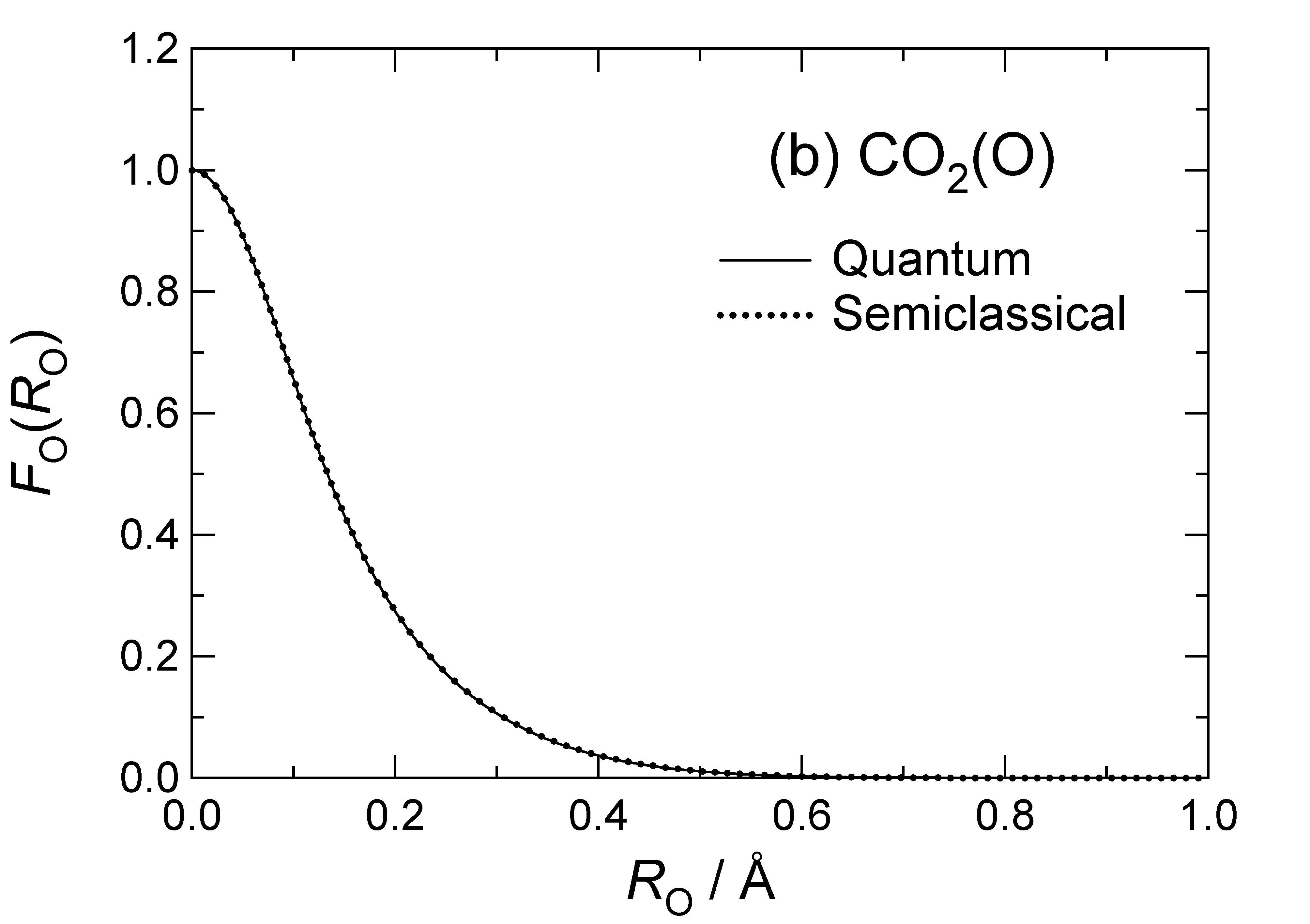
where is the zeroth-order spherical Bessel function. Fig. 6 shows the inverse Fourier transform of the momentum distributions of \ceH2O(H) and \ceCO2(O) calculated by Eq. 64. For comparison, also shown are the results calculated by using semiclassical for Eq. 64. In the case of \ceH2O(H), in the small region, the quantum and semiclassical results are almost identical to each other. However, as increases, there is a relevant deviation of the quantum result from the semiclassical one, as can be clearly seen in the insert of Fig. 6(a). In particular, the result of the quantum calculation exhibits a sharp decrease to zero at around . In the case of \ceCO2(O), there is no such a sharp decay; there is no appreciable difference in between the quantum and semiclassical results.
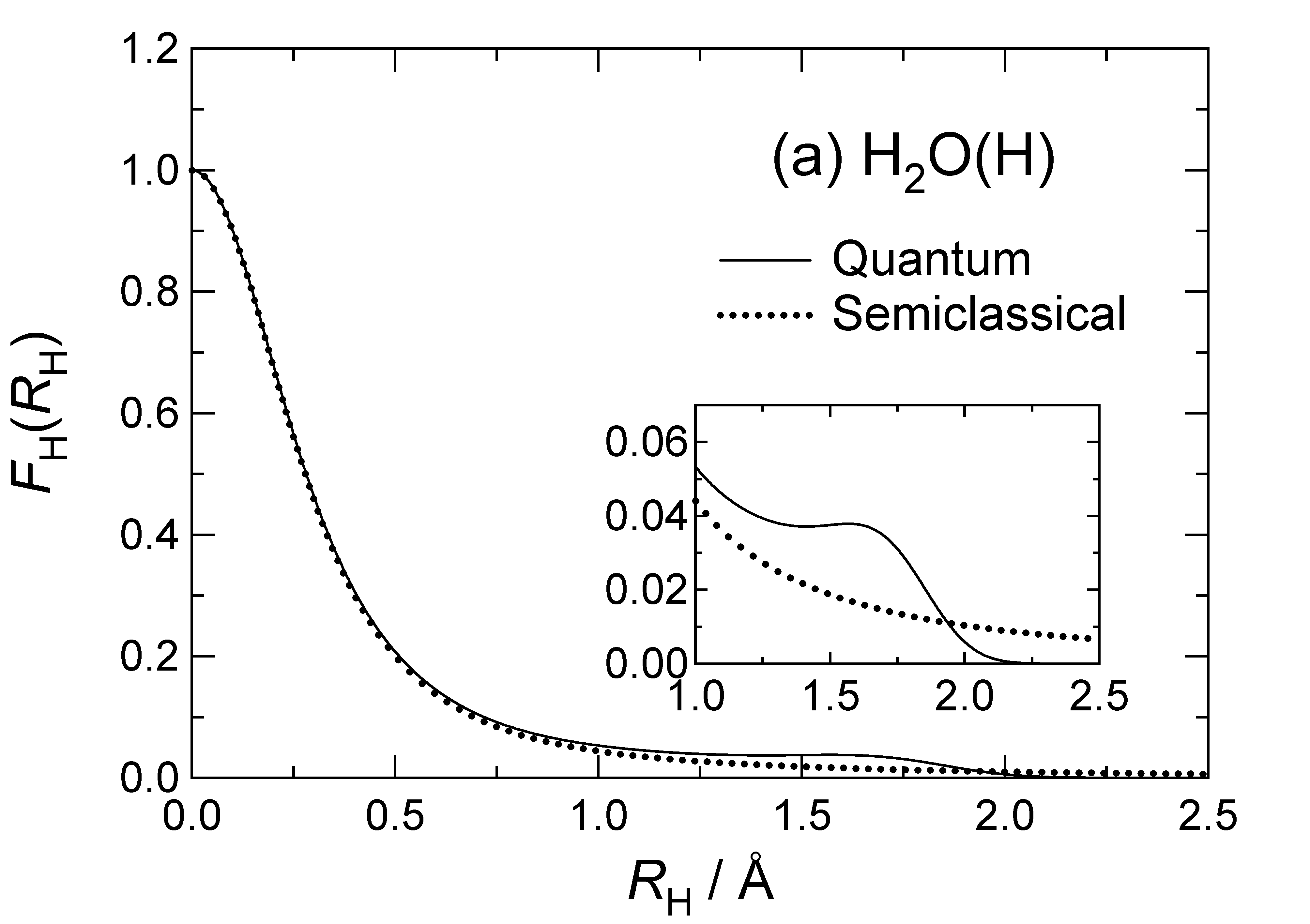
As mentioned in Section III in detail, the only difference between the quantum and semiclassical calculations is the treatment of rotational motion. In the small region, the autocorrelation is dominated by the overlap of the vibrational wavefunctions between the original and displaced positions. In this region, the semiclassical results are in good agreement with the quantum ones, as the semiclassical calculation can take into account the quantum-mechanical vibrational autocorrelation. Therefore, the difference in the between the quantum and semiclassical results of \ceH2O(H) demonstrates clearly the quantum effect of autocorrelation due to rotational motion, i.e., quantum rotational autocorrelation.
The sharp drop in the of \ceH2O(H), which does not appear in the semiclassical result, can be interpreted by the behavior of the autocorrelation in the rigid rotor model. To derive this model, we eliminate the effect of the translational motion in Eq. 62 by factorizing the autocorrelation function into the translational and rotational-vibrational parts.Colognesi et al. (2001) Substituting Eq. 57 into Eq. 62 (or Eq. 17 into Eq. 63), we obtain
| (65) |
where
| (66) | |||
| (67) |
with the position space satisfying . From Eq. 66, yields , which is consistent with Eq. 59. Thus, Eq. 65 becomes
| (68) |
In the same way as for the atomic momentum distribution, the rigid rotor model gives the autocorrelation function as
| (69) |
In general, as increases, deviates from the initial equilibrium configuration of the atoms, and hence the autocorrelation value decreases monotonically due to the decrease of the amplitude of the vibrational wavefunctions around . However, when a displaced atomic configuration accidentally coincides with the equilibrium molecular structure, the autocorrelation will retain a certain value. For \ceH2O, this situation is illustrated in Fig. 7(a). Quantum-mechanically, all the configurations in which the \ceH1 atom is on the dashed circle in Fig. 7(a) contribute to the autocorrelation coherently, since the \ceH1 atom is delocalized over the circle. On the other hand, there is no such rotational autocorrelation in the semiclassical calculation because the atomic momentum distribution within the semiclassical framework is obtained just by an orientational average (incoherent sum) of the atomic momentum distribution for one equilibrium configuration.Colognesi et al. (2001); Ivanov and Sayasov (1967) Therefore, it is concluded that the difference between the semiclassical and quantum results of for \ceH2O(H) is attributed to this rotational autocorrelation. It is noted that the upper limit of in the rotational autocorrelation is determined by the equilibrium molecular geometry of \ceH2O. It is , the diameter on which the \ceH1 atom is delocalized, corresponding to the position where the autocorrelation decays to zero in Fig. 6(a). In the case of \ceCO2, on the other hand, no rotational autocorrelation occurs because the displacement of the target \ceO1 atom always results in a different molecular structure from the stable linear structure, as shown in Fig. 7(b).
The above discussion about the quantum delocalization effect on the atomic momentum distributions can be extended to any molecule, not just to ground-state triatomic molecules. Another example is the oscillatory structure in the atomic momentum distribution of a diatomic molecule in the vibrational ground state. Since the oscillation is attributed to the spherical delocalization of the target atom around the other atom, diatomic molecules inherently exhibit the interference effect on the atomic momentum distribution. As mentioned in the Section I, it was pointed out that the wavelength (or period) of the oscillation depends on the internuclear distance.Colognesi and Pace (1999) This point can be revisited in terms of delocalization effect of the target atom with respect to the other atom; the internuclear distance determines the size of the sphere from which the plane waves are emitted.
V Conclusion
This study has reported the quantum theory for the atomic momentum distributions of polyatomic molecules, which is based on the momentum-space molecular wavefunctions in rotational-vibrational eigenstates. The rigid-rotor-harmonic-oscillator approximation has been developed to significantly reduce the computational cost, which enables one to extend the quantum-mechanical calculation to any kinds of isolated molecules in practice.
The proton momentum distribution in the ground-state \ceH2O was found to clearly show an oscillatory structure, or interference fringes. This oscillation is originated purely from the quantum nature and hence is not appeared on the momentum distribution when the molecular rotation is treated as classical. On the other hand, no such oscillation occurs on the oxygen momentum distribution in the ground-state \ceCO2 molecule even in the quantum calculation.
The rigid rotor model shows that whether or not the interference fringes appear in the atomic momentum distribution in a polyatomic molecule is determined by whether the target atom is delocalized or localized with respect to the other atoms. For the vibrational ground state, where the rigid rotor model is applicable, this finding leads to the following general rule that predicts necessarily the presence of interference fringes without rigorous calculations. Firstly, the positions of all atoms are fixed in an equilibrium configuration (initial configuration) of the molecule. Next, the target atom is displaced with keeping the other atoms in the same positions as the initial ones, to find one or more equilibrium configurations different from the initial configuration. Then, if the different equilibrium configurations are obtained, the interference structure may appear, otherwise no interference fringes are expected in the atomic momentum distribution.
Although a profound theoretical understanding for the delocalization effect on atomic momentum distributions has been gained for isolated molecules, experimental investigation has not been attempted so far. This is partially because the difficulty in a measurement on a single quantum state of dilute gas-phase molecules by using DINS, which has mostly been applied to condensed matter systems due to the limitation in sensitivity. However, the recent development of electron-atom Compton scattering, or Atomic Momentum Spectroscopy,Tachibana et al. (2022); Vos (2001); Cooper et al. (2007); Vos et al. (2013); Yamazaki et al. (2017); Onitsuka et al. (2022) would make it possible to measure the atomic momentum distribution in gas-phase molecules in their single quantum state. A combination of a recently developed highly-sensitive apparatusYamazaki et al. (2017) with adiabatic cooling would offer a promising means of studying the quantum effects on the atomic momentum distribution in a single molecule, and the observation of the oscillatory structure in a rovibrational state would become feasible in the near future.
*
Appendix A Simplification of the Jacobian
Nonlinear molecules
From Eqs. 9 and 24, the derivatives of the mass-weighted coordinates with respect to the generalized coordinates become
| (70) |
with , and hence we can write the Jacobian matrix as
| (71) |
where all bold symbols represent column vectors, and the directions of the infinitesimal rotation vector , , and are given by
| (72a) | ||||
| (72b) | ||||
| (72c) | ||||
and is the direct sum of rotation matrices in three dimensions . Using Eq. 23 and the translational Eckart conditions
| (73) |
we can simplify the determinant of Eq. 4b to
| (74) |
where is the identity matrix of size , and the matrix and the matrix are written as
| (75) | |||
| (76) |
with the matrix and . From Eqs. 75 and 76, we obtain
| (77) |
Substituting Eq. 77 into Eq. 74, is rewritten as
| (78) |
where we use . Calculating Eq. 4a from , the determinant is
| (79) |
Therefore, can be expressed as
| (80) |
Linear molecules
As mentioned above, for linear molecules, the Euler angle in the rotation matrix is set as . Thus, the derivatives of are
| (81) |
which yield
| (82) |
In this case, and are written as
| (83a) | ||||
| (83b) | ||||
In the same way as for nonlinear molecules, we obtain
| (84) |
where the matrix and the matrix is given by
| (85) | |||
| (86) |
with the matrix . From Eqs. 85 and 86, we have
| (87) |
where we use Eq. 31. Substituting Eq. 87 into Eq. 84, we can rewrite as
| (88) |
Therefore, for linear molecules can be expressed as
| (89) |
Acknowledgements.
This work was partially supported by JSPS KAKENHI Grant Number JP20H02688. It was also supported in part by the Inamori Research Grants, the Research Foundation for Opto-Science and Technology, the MATSUO FOUNDATION, and the Institute for Quantum Chemical Exploration. This work was also partially supported by JST FOREST Program (Grant Number JPMJFR201X, Japan).References
- Ceriotti et al. (2016) M. Ceriotti, W. Fang, P. G. Kusalik, R. H. McKenzie, A. Michaelides, M. A. Morales, and T. E. Markland, Chemical Reviews 116, 7529 (2016).
- Tuckerman and Ceperley (2018) M. Tuckerman and D. Ceperley, The Journal of Chemical Physics 148, 102001 (2018).
- Fang et al. (2019) W. Fang, J. Chen, Y. Feng, X.-Z. Li, and A. Michaelides, International Reviews in Physical Chemistry 38, 35 (2019).
- Evans et al. (1993) A. C. Evans, J. Mayers, D. N. Timms, and M. J. Cooper, Zeitschrift für Naturforschung A 48, 425 (1993), publisher: De Gruyter.
- Watson (1996) G. I. Watson, Journal of Physics: Condensed Matter 8, 5955 (1996).
- Mayers et al. (2002) J. Mayers, G. Reiter, and P. Platzman, Journal of Molecular Structure 615, 275 (2002).
- Andreani et al. (2005) C. Andreani, D. Colognesi, J. Mayers, G. F. Reiter, and R. Senesi, Advances in Physics 54, 377 (2005).
- Andreani et al. (2017) C. Andreani, M. Krzystyniak, G. Romanelli, R. Senesi, and F. Fernandez-Alonso, Advances in Physics 66, 1 (2017).
- Reiter et al. (2002) G. F. Reiter, J. Mayers, and P. Platzman, Physical Review Letters 89, 135505 (2002).
- Reiter et al. (2012) G. F. Reiter, A. I. Kolesnikov, S. J. Paddison, P. M. Platzman, A. P. Moravsky, M. A. Adams, and J. Mayers, Physical Review B 85, 045403 (2012).
- Garbuio et al. (2007) V. Garbuio, C. Andreani, S. Imberti, A. Pietropaolo, G. F. Reiter, R. Senesi, and M. A. Ricci, The Journal of Chemical Physics 127, 154501 (2007).
- Senesi et al. (2007) R. Senesi, A. Pietropaolo, A. Bocedi, S. E. Pagnotta, and F. Bruni, Physical Review Letters 98, 138102 (2007).
- Reiter et al. (2004) G. Reiter, J. C. Li, J. Mayers, T. Abdul-Redah, and P. Platzman, Brazilian Journal of Physics 34, 142 (2004).
- Kolesnikov et al. (2016) A. I. Kolesnikov, G. F. Reiter, N. Choudhury, T. R. Prisk, E. Mamontov, A. Podlesnyak, G. Ehlers, A. G. Seel, D. J. Wesolowski, and L. M. Anovitz, Physical Review Letters 116, 167802 (2016).
- Reiter and Silver (1985) G. Reiter and R. Silver, Physical Review Letters 54, 1047 (1985).
- Andreani et al. (2001) C. Andreani, E. Degiorgi, R. Senesi, F. Cilloco, D. Colognesi, J. Mayers, M. Nardone, and E. Pace, The Journal of Chemical Physics 114, 387 (2001).
- Homouz et al. (2007) D. Homouz, G. Reiter, J. Eckert, J. Mayers, and R. Blinc, Physical Review Letters 98, 115502 (2007).
- Flammini et al. (2012) D. Flammini, A. Pietropaolo, R. Senesi, C. Andreani, F. McBride, A. Hodgson, M. A. Adams, L. Lin, and R. Car, The Journal of Chemical Physics 136, 024504 (2012).
- Soper (2009) A. K. Soper, Physical Review Letters 103, 069801 (2009).
- Lin et al. (2011) L. Lin, J. A. Morrone, R. Car, and M. Parrinello, Physical Review B 83, 220302 (2011).
- Wu and Car (2020) Y. Wu and R. Car, The Journal of Chemical Physics 152, 024106 (2020).
- Morrone and Car (2008) J. A. Morrone and R. Car, Physical Review Letters 101, 017801 (2008).
- Lin et al. (2010) L. Lin, J. A. Morrone, R. Car, and M. Parrinello, Physical Review Letters 105, 110602 (2010).
- Ceriotti and Manolopoulos (2012) M. Ceriotti and D. E. Manolopoulos, Physical Review Letters 109, 100604 (2012).
- Colognesi and Pace (1999) D. Colognesi and E. Pace, Physica B: Condensed Matter 266, 267 (1999).
- Andreani et al. (1995) C. Andreani, A. Filabozzi, and E. Pace, Physical Review B 51, 8854 (1995).
- Tachibana et al. (2022) Y. Tachibana, Y. Onitsuka, H. Kono, and M. Takahashi, Physical Review A 105, 052813 (2022).
- Colognesi et al. (2001) D. Colognesi, E. Degiorgi, and E. Pace, Physica B: Condensed Matter 293, 317 (2001).
- Wilson et al. (1955) E. B. Wilson, J. Decius, and P. C. Cross, Molecular Vibrations : The Theory of Infrared and Raman Vibrational Spectra, Vibrational spectra (McGraw-Hill, New York, United States, 1955).
- Bunker and Jensen (2006) P. R. Bunker and P. Jensen, Molecular Symmetry and Spectroscopy (NRC Research Press, 2006).
- Podolsky (1928) B. Podolsky, Physical Review 32, 812 (1928).
- Watson (1970) J. K. Watson, Molecular Physics 19, 465 (1970).
- Watson (1968) J. K. Watson, Molecular Physics 15, 479 (1968).
- Eckart (1935) C. Eckart, Physical Review 47, 552 (1935).
- Amat and Henry (1958) G. Amat and L. Henry, Cahiers de Physique 12, 273 (1958).
- Frisch et al. (2016) M. J. Frisch, G. W. Trucks, H. B. Schlegel, G. E. Scuseria, M. A. Robb, J. R. Cheeseman, G. Scalmani, V. Barone, G. A. Petersson, H. Nakatsuji, X. Li, M. Caricato, A. V. Marenich, J. Bloino, B. G. Janesko, R. Gomperts, B. Mennucci, H. P. Hratchian, J. V. Ortiz, A. F. Izmaylov, J. L. Sonnenberg, D. Williams-Young, F. Ding, F. Lipparini, F. Egidi, J. Goings, B. Peng, A. Petrone, T. Henderson, D. Ranasinghe, V. G. Zakrzewski, J. Gao, N. Rega, G. Zheng, W. Liang, M. Hada, M. Ehara, K. Toyota, R. Fukuda, J. Hasegawa, M. Ishida, T. Nakajima, Y. Honda, O. Kitao, H. Nakai, T. Vreven, K. Throssell, J. A. Montgomery, Jr., J. E. Peralta, F. Ogliaro, M. J. Bearpark, J. J. Heyd, E. N. Brothers, K. N. Kudin, V. N. Staroverov, T. A. Keith, R. Kobayashi, J. Normand, K. Raghavachari, A. P. Rendell, J. C. Burant, S. S. Iyengar, J. Tomasi, M. Cossi, J. M. Millam, M. Klene, C. Adamo, R. Cammi, J. W. Ochterski, R. L. Martin, K. Morokuma, O. Farkas, J. B. Foresman, and D. J. Fox, “Gaussian˜16 Revision C.01,” (2016), gaussian Inc. Wallingford CT.
- Ivanov and Sayasov (1967) G. Ivanov and Yu.S. Sayasov, Soviet Physics Uspekhi 9, 670 (1967).
- Cullity and Stock (2001) B. Cullity and S. Stock, Elements of X-ray Diffraction, Third Edition (Prentice-Hall, New York, 2001).
- Waseda et al. (2011) Y. Waseda, E. Matsubara, and K. Shinoda, in X-Ray Diffraction Crystallography: Introduction, Examples and Solved Problems, edited by Y. Waseda, E. Matsubara, and K. Shinoda (Springer, Berlin, Heidelberg, 2011) pp. 67–106.
- Vos (2001) M. Vos, Physical Review A 65, 012703 (2001).
- Cooper et al. (2007) G. Cooper, E. Christensen, and A. P. Hitchcock, The Journal of Chemical Physics 127, 084315 (2007).
- Vos et al. (2013) M. Vos, E. Weigold, and R. Moreh, The Journal of Chemical Physics 138, 044307 (2013).
- Yamazaki et al. (2017) M. Yamazaki, M. Hosono, Y. Tang, and M. Takahashi, Review of Scientific Instruments 88, 063103 (2017).
- Onitsuka et al. (2022) Y. Onitsuka, Y. Tachibana, and M. Takahashi, Physical Chemistry Chemical Physics 24, 19716 (2022).