Black Box Differential Privacy Auditing
Using Total Variation Distance

Abstract

We present a practical method to audit the differential privacy (DP) guarantees of a machine learning model using a small hold-out dataset that is not exposed to the model during the training. Having a score function such as the loss function employed during the training, our method estimates the total variation (TV) distance between scores obtained with a subset of the training data and the hold-out dataset. With some meta information about the underlying DP training algorithm, these TV distance values can be converted to $(\varepsilon,\delta)$-guarantees for any $\delta$. We show that these score distributions asymptotically give lower bounds for the DP guarantees of the underlying training algorithm, however, we perform a one-shot estimation for practicality reasons. We specify conditions that lead to lower bounds for the DP guarantees with high probability. To estimate the TV distance between the score distributions, we use a simple density estimation method based on histograms. We show that the TV distance gives a very close to optimally robust estimator and has an error rate $\mathcal{O}(k^{-1/3})$, where $k$ is the total number of samples. Numerical experiments on benchmark datasets illustrate the effectiveness of our approach and show improvements over baseline methods for black-box auditing.

1 Introduction

Differential Privacy (Dwork et al.,, 2006) (DP) limits the disclosure of membership information of individuals in statistical data analysis. It has been successfully applied also to the training of machine learning (ML) models, where the de facto standard is the DP stochastic gradient descent (DP-SGD) (see e.g., Abadi et al.,, 2016). DP-SGD enables the analysis of the formal $(\varepsilon,\delta)$-DP guarantees via composition analysis in a threat model where the guarantees hold against an adversary that has the access to the whole history of models. Besides, it is possible to obtain accurate $(\varepsilon,\delta)$-DP guarantees for DP-SGD using numerical accounting tools (Koskela et al.,, 2020; Zhu et al.,, 2022; Gopi et al.,, 2021).

We motivate the privacy auditing problem by the following scenario. Consider a federated learning setup, where a non-fully-trusted server participates in enhancing the DP protection to provide better privacy-utility trade-off for the final model. In order to achieve the theoretical privacy guarantees of DP-SGD, a notoriously difficult implementation setup is needed (Tramer et al.,, 2022; Nasr et al.,, 2023). Since parts of the model updates are performed by an external entity, there is no full certainty for the data-owner that the DP guarantees hold (see e.g. Maddock et al.,, 2023; Andrew et al.,, 2024, for methods addressing this). The question then is, how could the data owner perform privacy auditing during the training? And how could the auditing be performed in a setting where only a black-box access to the model is available?

The problem of privacy auditing has increasingly gained attention during recent years. Many of the existing works on DP auditing focuses on inserting well-designed data elements or gradients into the training dataset, coined as the canaries. By observing their effect later in the trained model one can infer about the DP guarantees (see, e.g., Jagielski et al.,, 2020; Nasr et al.,, 2021; Pillutla et al.,, 2023). These methods commonly also require training several models in order to obtain the estimates of the DP guarantees, even up to thousands (Pillutla et al.,, 2023). To overcome the computational burden of training the model multiple times, recently Steinke et al., (2023) and Andrew et al., (2024) have proposed different approaches that requires access to only a single model.

Similarly to Steinke et al., (2023), we audit the model by using a small hold-out dataset. Moreover, we focus on inferring the DP guarantees from the final model. Our method is also related to the threshold membership inference attacks (Yeom et al.,, 2018; Carlini et al.,, 2022) and also to the memorization exposure metric considered by Carlini et al., (2019). In the FL setting, there are two notable works related to ours, both of which are heuristic methods based on estimating the $(\varepsilon,\delta)$-distance between Gaussian distributions (Andrew et al.,, 2024; Maddock et al.,, 2023). The work by Andrew et al., (2024) advocates for inserting randomly sampled canaries in the model updates, which could deteriorate the model accuracy. Moreover, their method requires a white-box access to the model. The work by (Maddock et al.,, 2023) is based on carefully crafting canary gradients that are inserted in the model updates.

We focus on a scenario where the auditor only has a black-box access to the model via its predictions. Furthermore, the auditor has access to the auditing training and test data samples, i.e., to auditing data samples that used for the training and that are held out, respectively. This fits particularly well to practical federated learning (FL) scenarios, where, e.g., a data owner may want to find out whether the central aggregator has fulfilled the DP guarantees as advertised. We further assume no engineered canary data is injected to the training dataset. We propose to use a score function, such as the loss function used for the training, to measure the model’s performance. We mathematically show that the empirical $\varepsilon$-values obtained with threshold membership inference attacks based on the score values are equivalent to measuring the hockey-stick divergence between the two discrete distributions obtained by a simple two-bin histogram frequency estimation of the score values corresponding to the auditing training and tests sets, respectively. Our novelty is to use multiple bins for for the frequency estimation of these two distributions. The rational behind our method is similar to the one from the threshold membership inference attacks in that we compute a finite-sample one-shot estimate of the score distributions, by assuming independence between the score values corresponding to the auditing training and test sets (Zanella-Béguelin et al.,, 2023). Analyses that avoid this assumption can be found in (Steinke et al.,, 2023) and (Pillutla et al.,, 2023). Our approach allows using any hockey-stick divergence to measure the distance between the score distributions of auditing training and test samples. We analytically prove that the optimal hockey-stick divergence distance parameter $\alpha$, which leads to the most robust estimate of the distance and thus the $(\varepsilon,\delta)$-estimates, occurs at the vicinity of $\alpha=1$, which corresponds to the total variation distance.

After giving the necessary definitions on differential privacy, in Section 3 we first describe the idea of obtaining $(\varepsilon,\delta)$-DP lower bounds via the hockey-stick divergence between the score distributions of the auditing training and test samples. In Section 4, we show how to numerically estimate the hockey-stick divergence between those distributions using histogram density estimators. Then, in Section 5 we analytically illustrate that the total variation distance gives a robust estimator for the distance between two Gaussian distributions, which is practically relevant for estimating the $(\varepsilon,\delta)$-DP lower bounds for DP-SGD trained models. Experiments in Section 7 illustrate the effectiveness of the proposed auditing method for which a pseudocode is listed in Section 6.

2 Required Background on Differential Privacy

We first give the preliminaries for the techniques based on hockey-stick divergence, and in particular for the special case of the total variation distance.

We denote the space of possible data points by $X$. We denote a dataset containing $n$ data points as $D=(x_{1},\ldots,x_{n})\in X^{n}$, and the space of all possible datasets (of all sizes) by $\mathcal{X}$. We say $D$ and $D^{\prime}$ are neighboring datasets if we get one by substituting one element in the other. We say that a mechanism $\mathcal{M}\,:\,\mathcal{X}\rightarrow\mathcal{O}$ is $(\varepsilon,\delta)$-DP if the output distributions for neighboring datasets are always $(\varepsilon,\delta)$-indistinguishable.

Definition 1.

Let $\varepsilon\geq 0$ and $\delta\in[0,1]$. Mechanism $\mathcal{M}\,:\,\mathcal{X}\rightarrow\mathcal{O}$ is $(\varepsilon,\delta)$-DP if for every pair of neighboring datasets $D,D^{\prime}\in\mathcal{X}$ and every measurable set $E\subset\mathcal{O}$,

$$\mathbb{P}(\mathcal{M}(D)\in E)\leq{\rm e}\hskip 1.0pt^{\varepsilon}\mathbb{P}(\mathcal{M}(D^{\prime})\in E)+\delta.$$

We call $\mathcal{M}$ tightly $(\varepsilon,\delta)$-DP, if there does not exist $\delta^{\prime}<\delta$ such that $\mathcal{M}$ is $(\varepsilon,\delta^{\prime})$-DP.

The tight $(\varepsilon,\delta)$-guarantees can be equivalently formulated using the hockey-stick divergence. For $\alpha\geq 0$ the hockey-stick divergence $H_{\alpha}$, also called the $\alpha$-divergence, from a distribution $P$ to a distribution $Q$ is defined as

$$H_{\alpha}(P||Q)=\int\left[P(t)-\alpha\cdot Q(t)\right]_{+}\,\hskip 1.0pt{\rm d}\hskip 0.5ptt,$$ (2.1)

where for $t\in\mathbb{R}$, $[t]_{+}=\max\{0,t\}$. The $(\varepsilon,\delta)$-DP guarantees as in Definition 1 can be characterized using the hockey-stick divergence as follows.

Lemma 2 (Balle et al., 2018, Theorem 1).

For a given $\varepsilon\in\mathbb{R}$, a mechanism $\mathcal{M}$ satisfies $(\epsilon,\delta)$-DP if and only if, for all neighboring datasets $D,D^{\prime}$,

$$H_{{\rm e}\hskip 1.0pt^{\varepsilon}}(\mathcal{M}(D)||\mathcal{M}(D^{\prime}))\leq\delta.$$

By Lemma 2, if we can bound $H_{{\rm e}\hskip 1.0pt^{\varepsilon}}(\mathcal{M}(D)||\mathcal{M}(D^{\prime}))$ accurately for all neighboring datasets $D,D^{\prime}$, we also obtain accurate $(\varepsilon,\delta)$-DP bounds. For compositions of general DP mechanisms, this can be carried out by using so-called dominating pairs of distributions (Zhu et al.,, 2022) and numerical techniques (Koskela et al.,, 2021; Gopi et al.,, 2021). In some cases, such as for the Gaussian mechanism, the hockey-stick divergence (2.1) leads to analytical expressions for tight $(\varepsilon,\delta)$-DP guarantees (see, e.g., Balle and Wang,, 2018).

Lemma 3.

Let $d_{0},d_{1}\in\mathbb{R}^{d}$, $\sigma\geq 0$, and let $P$ be the density function of $\mathcal{N}(d_{0},\sigma^{2}I_{d})$ and $Q$ the density function of $\mathcal{N}(d_{1},\sigma^{2}I_{d})$. Then, for all $\varepsilon\in\mathbb{R}$, the divergence $H_{{\rm e}\hskip 1.0pt^{\varepsilon}}(P||Q)$ is given by the expression

$$\delta(\varepsilon)=\Phi\left(-\frac{\varepsilon\sigma}{\Delta}+\frac{\Delta}{2\sigma}\right)-e^{\varepsilon}\Phi\left(-\frac{\varepsilon\sigma}{\Delta}-\frac{\Delta}{2\sigma}\right),$$ (2.2)

where $\Phi$ denotes the CDF of the standard univariate Gaussian distribution and $\Delta=\|d_{0}-d_{1}\|_{2}$.

Total variation distance.

Setting $\alpha=1$ in Eq. (2.1), we get the TV distance between the probability distributions $P$ and $Q$ (see e.g., Sec. 2.4, Balle et al.,, 2020),

$$\mathrm{TV}(P,Q)=\frac{1}{2}\int\left|P(x)-Q(x)\right|\,\hskip 1.0pt{\rm d}\hskip 0.5ptx=\int[P(x)-Q(x)]_{+}\,\hskip 1.0pt{\rm d}\hskip 0.5ptx.$$ (2.3)

When $P$ and $Q$ are discrete, defined by probabilities $p_{k}$ and $q_{k}$, $k\in\mathbb{Z}$, respectively, we have the important special case of discrete TV distance defined by

$$\mathrm{TV}(P,Q)=\sum_{k\in\mathbb{Z}}\max\{p_{k}-q_{k},0\}.$$

3 Empirical DP Guarantees Using Score Functions

3.1 Score Functions

We define score function $S$ as a deterministic real-valued function associated to a randomized function $\mathcal{M}\,:\,\mathcal{X}\rightarrow\mathcal{O}$ as $S\,:\,\mathcal{O}\times X\rightarrow\mathbb{R}$, where, for a given $\theta\in\mathcal{O}$ (e.g., ML model parameters) and $x\in X$ (a data element), $S(\theta,x)$ gives a score value. As an example, if $\theta\in\mathbb{R}^{d}$ denotes the model parameters, $F(\theta,z)$ the forward mapping for the features $z$ of a data element $x=(z,y)\in X$, where $y$ denotes the label, we may consider the score

$$S(\theta,x)=\ell\big{(}F(\theta,z),y\big{)},$$

where $\ell\big{(}F(\theta,z),y\big{)}$ is some loss function.

3.2 Motivation and Relation to Existing Work

As a motivation, we first consider a simple threshold membership inference attack which can be seen as a special case of our auditing method. Let us denote the total auditing dataset by $A$ and the auditing training dataset by $D$. Thus, the auditing test dataset, i.e., the hold-out auditing dataset, equals $A\setminus D$. Suppose that we are given some score function $S$ and a fixed threshold $\tau$. We infer that a sample is in the auditing training set in case its score is below $\tau$. This gives the true positive ratios (TPRs) and false positive ratios (FPRs)

$$\mathrm{TPR}=\mathbb{P}_{x\sim D}\left(S(\theta,x)<\tau\right),\quad\quad\mathrm{FPR}=\mathbb{P}_{x\sim A\setminus D}\left(S(\theta,x)<\tau\right),$$ (3.1)

where $x\sim D$ denotes that $x$ is uniformly randomly sampled from $D$. As is common, estimates of $\mathrm{TPR}$- and $\mathrm{FPR}$-values can further be used to estimate lower bounds for the $(\varepsilon,\delta)$-privacy parameters. We can interpret the $(\varepsilon,\delta)$-estimates given by this threshold membership inference as the $(\varepsilon,\delta)$-distance between two-bin approximations (bins defined by the parameter $\tau\in\mathbb{R}$ dividing the real line into two bins) of the distributions $P$ and $Q$, where $P$ and $Q$ are defined as

$$P=S(\mathcal{M}(D),x),\quad x\sim D,\quad\quad Q=S(\mathcal{M}(D),x),\quad x\sim A\setminus D.$$ (3.2)

Let $P_{2}$ and $Q_{2}$ denote the two-bin histogram approximations of $P$ and $Q$, respectively, where the bins are determined by the threshold parameter $\tau$. The following lemma shows that the $(\varepsilon,\delta)$-distance between $P_{2}$ and $Q_{2}$ exactly matches with the expression commonly used for the empirical $\varepsilon$-values.

Lemma 1.

Let $A$ be the auditing set, $D\subset A$ the auditing training set and $A\setminus D$ the auditing test set. Consider the distributions $P$ and $Q$ as defined in Eq. (3.2) and distributions $P_{2}$ and $Q_{2}$ obtained with two-bin frequency histograms defined by a threshold $\tau\in\mathbb{R}$. Suppose the underlying mechanism $\mathcal{M}$ is $(\varepsilon,\delta)$-DP for some $\varepsilon\geq 0$ and $\delta\in[0,1]$. Then,

$$\max\{H_{{\rm e}\hskip 1.0pt^{\varepsilon}}\big{(}P_{2}||Q_{2}\big{)},H_{{\rm e}\hskip 1.0pt^{\varepsilon}}\big{(}Q_{2}||P_{2}\big{)}\}=\delta,$$

where

$$\varepsilon=\max\left\{\log\frac{\mathrm{TPR}-\delta}{\mathrm{FPR}},\log\frac{\mathrm{TNR}-\delta}{\mathrm{FNR}}\right\}.$$ (3.3)

and $\mathrm{TPR}$ and $\mathrm{FPR}$ are as defined in Eq. (3.1) and $\mathrm{FNR}=1-\mathrm{TPR}$ and $\mathrm{TNR}=1-\mathrm{FPR}$.

The $\varepsilon$-estimate of Eq.(3.3) is exactly the characterization given by Kairouz et al., (2015) for the connection between the success rates of membership inference attacks and the $(\varepsilon,\delta)$-DP guarantees of the underlying mechanism. Our novelty is to generalize this threshold membership inference auditing such that we consider histograms with more than two bins, and instead of estimating TPRs and FPRs, we estimate the relative frequencies of the scores hitting each of the bins and then measure the $(\varepsilon,\delta)$-distance between the approximated distributions corresponding to the score distributions of the two auditing sets. We remark that the auditing training and test sample scores would generally need to be independent to conclude that the estimate of Eq.(3.3) gives a lower bound for the actual $(\varepsilon,\delta)$-DP guarantees (see also the discussion in Jagielski,, 2023).

Following the discussion of Jagielski, (2023), we see that our approach is also related to the exposure metric defined by Carlini et al., (2019). Given $n$ auditing training samples $\{c_{i}\}_{i=1}^{n}$ and $n$ auditing test samples $\{r_{i}\}_{i=1}^{n}$, Carlini et al., (2019) defines the exposure of a sample $c_{i}$ via its rank

$$\mathrm{Exposure}(c_{i})=\log_{2}n-\log_{2}\mathrm{rank}(c_{i},\{r_{i}\}_{i=1}^{n}),$$

where $\mathrm{rank}(c_{i},\{r_{i}\}_{i=1}^{n})$ equals the number of auditing test samples with loss smaller then the loss of $c_{i}$. As Jagielski, (2023) shows, a reasonable approximation for the the expected exposure is given by the threshold membership inference (i.e., a two-bin histogram approximation desribed above) with threshold parameter $\tau=\ell_{\mathrm{median}}$, where $\ell_{\mathrm{median}}$ is the median value of the losses of the auditing training samples, i.e., the median of $\{\ell(c_{i})\}_{i=1}^{n}$. This leads to the $\varepsilon$-estimate given by Eq. (3.3) with $\mathrm{TPR}=\mathbb{P}_{x\sim D}\left(\ell(x)<\ell_{\mathrm{median}}\right)$ and $\mathrm{FPR}=\mathbb{P}_{x\sim A\setminus D}\left(\ell(x)<\ell_{\mathrm{median}}\right).$ We remark that the rigorous lower bounds given by Steinke et al., (2023) can also be seen as approximations of this form.

3.3 Distinguishability of the Estimated Scores

Let $A$ denote the auditing dataset and $D\subset A$ the auditing training set, as above. The DP property of the mechanisms $\mathcal{M}$ suggests that the distributions

$$P=S(\mathcal{M}(D),x),\quad x\sim D,\quad\quad\quad Q=S(\mathcal{M}(D),x),\quad x\sim A\setminus D$$ (3.4)

should be $(\varepsilon,\delta)$-close to each other. In the following result, we show that when letting $D$ also be a random variable, independently for $P$ and $Q$, the distributions $P$ and $Q$ are $(\varepsilon,\delta)$-close in case the mechanism $\mathcal{M}$ is $(\varepsilon,\delta)$-DP. By the post-processing property of the hockey-stick divergence, this result hold for any score function $S$.

Theorem 2.

Let $A\subset X^{n}$ where $|A|$ is even, denote the total auditing set, and suppose the mechanism $\mathcal{M}$ is $(\varepsilon,\delta)$-DP. Denote

$$\widetilde{P}=S(\theta,x),\quad\textrm{where}\quad\theta\sim\mathcal{M}(D),\,D\sim\mathrm{Subsample}(A),\,x\sim D$$

and

$$\widetilde{Q}=S(\theta,x),\quad\textrm{where}\quad\theta\sim\mathcal{M}(D),\,D\sim\mathrm{Subsample}(A),\,x\sim A\setminus D,$$

where $\mathrm{Subsample}(A)$ randomly samples half of the set $A$ without replacement. Then,

$$\max\left\{H_{{\rm e}\hskip 1.0pt^{\varepsilon}}\big{(}\widetilde{P}||\widetilde{Q}\big{)},H_{{\rm e}\hskip 1.0pt^{\varepsilon}}\big{(}\widetilde{Q}||\widetilde{P}\big{)}\right\}\leq\delta.$$

Theorem 2 states that the distributions of score values estimated at the auditing training and auditing test sets are $(\varepsilon,\delta)$-close in case the underlying mechanism $\mathcal{M}$ is $(\varepsilon,\delta)$-DP and also the randomness of drawing the auditing training set $D\subset A$ is also included in the score distributions. Our aim, however, is to carry out the auditing of $(\varepsilon,\delta)$-values using a single draw of $D$.

The following result gives an example of a high-dimensional mechanism, where the approach of estimating $(\varepsilon,\delta)$-distance between one-dimensional score distributions $P$ and $Q$ (as defined in Eq. (3.4)) gives the $(\varepsilon,\delta)$-guarantees for the underlying mechanism $\mathcal{M}$ with high probability.

Theorem 3.

Suppose the dataset $X=\{x_{1},\ldots,x_{n}\}$, where $x_{i}$’s are i.i.d. uniformly sampled from the unit sphere $\mathbb{S}^{d-1}$. Suppose $\mathcal{M}$ is the DP mean estimation mechanism, i.e.,

$$\mathcal{M}(X)=\sum_{x\in X}x+Z,\quad Z\sim\mathcal{N}(0,\sigma^{2}),$$

where $\sigma>0$ is chosen such that for a given dataset $X$, $\mathcal{M}$ is tightly $(\varepsilon,\delta)$-DP. Let the score function $S$ be defined as $S(\theta,x)=\theta^{T}x$. Let $P$ and $Q$ be as defined in Eq. (3.4) using a random $D\subset A$, $\left|D\right|=\left|A\right|/2$. Then, for any $\tau>0$,

$$\mathbb{P}\left(\left|H_{{\rm e}\hskip 1.0pt^{\varepsilon}}\big{(}P||Q\big{)}-\delta\right|>\tau\right)\rightarrow 0\quad\textrm{as}\quad d\rightarrow\infty.$$

The following result states that if the mechanism $\mathcal{M}$ is stable in a sense that the average total variation distance between the test errors, respectively training errors, for two models trained on neighboring datasets is $\mathcal{O}(\delta)$ with high probability w.r.t. sampling of the auditing training set $D\subset A$, and the mechanism $\mathcal{M}$ is $(\varepsilon,\delta)$-DP, then one training run gives us a good approximation of the lower bound of the $(\varepsilon,\delta)$-values. Notice that the conditions of Lemma 4 can be seen as stability conditions for the training and test losses and are thus very different than, for example, the average generalization error (see, e.g., Yeom et al.,, 2018).

Theorem 4.

Let $\tau>0$. Suppose that with probability $1-\tau$ w.r.t. to the randomness of sampling $D\subset A$, for some $\widehat{\delta}>0$, for all measurable $E\subset\mathbb{R}$,

$$\mathbb{P}_{x^{\prime}\sim A\setminus D,x\sim D}\big{(}S(\mathcal{M}(D\setminus\{x\}\cup\{x^{\prime}\}),x)\in E\big{)}-\mathbb{P}_{x\sim A\setminus D}\big{(}S(\mathcal{M}(D),x)\in E\big{)}\leq\widehat{\delta}$$

and suppose $\mathcal{M}$ is $(\varepsilon,\delta)$-DP for some $\varepsilon\in\mathbb{R}$. Then, for $P$ and $Q$ as defined in Eq. (3.4), we have with probability $1-\tau$,

$$H_{{\rm e}\hskip 1.0pt^{\varepsilon}}\big{(}P||Q\big{)}\leq\delta+{\rm e}\hskip 1.0pt^{\varepsilon}\cdot\widehat{\delta}.$$

Suppose that with probability $1-\tau$ w.r.t. to the randomness of sampling $D\subset A$, for some $\widehat{\delta}>0$, for all measurable $E\subset\mathbb{R}$,

$$\mathbb{P}_{x\sim A\setminus D,x^{\prime}\sim D}\big{(}S(\mathcal{M}(D\setminus\{x^{\prime}\}\cup\{x\}),x)\in E\big{)}-\mathbb{P}_{x\sim D}\big{(}S(\mathcal{M}(D),x)\in E\big{)}\leq\widehat{\delta}$$

and suppose $\mathcal{M}$ is $(\varepsilon,\delta)$-DP for some $\varepsilon\in\mathbb{R}$. Then, for $P$ and $Q$ as defined in Eq. (3.4), we have with probability $1-\tau$,

$$H_{{\rm e}\hskip 1.0pt^{\varepsilon}}\big{(}Q||P\big{)}\leq\delta+{\rm e}\hskip 1.0pt^{\varepsilon}\cdot\widehat{\delta}.$$

4 Estimating Densities of the Score Distributions

We next consider a method for one-shot estimation of the hockey-stick divergence $H_{\alpha}(\widetilde{P}||\widetilde{Q})$, $\alpha\geq 0$, where $\widetilde{P}$ and $\widetilde{Q}$ are as defined in Eq. (3.4). This is carried out via histogram density estimates constructed using the samples from the score distributions $P$ and $Q$ defined in Eq. (3.2)

4.1 Density Estimation Using Histograms

Given the auditing training set $A$, we estimate the $\widetilde{P}$ and $\widetilde{Q}$ defined in Eq. (3.4) by first sampling the auditing training set $D$ (denoted $A_{\mathrm{train}}$ from now on) from $A$ and by evaluating the scores of the $k$ samples of $A_{\mathrm{train}}$ and of the $k$ samples of the auditing test set $A_{\mathrm{test}}:=A\setminus A_{\mathrm{train}}$. Then, we carry out a binning such that we place the score values into $N$ bins, each of width $h>0$. Given the left and right end points $a$ and $b$, respectively, we define the bin $j$, $j\in[N-1]$, as

$$\textrm{Bin}_{j}=[a+(j-1)\cdot h,a+j\cdot h)$$

and

$$\textrm{Bin}_{N}=[b-h,b].$$

After training the machine learning model (i.e., evaluate $\mathcal{M}(A_{\mathrm{train}})=\theta$), we estimate the probabilities $p_{j}$ and $q_{j}$, $j\in[N]$, by the relative frequencies of hitting bin $j$:

$$p_{j}\leftarrow\frac{\#\{x\in A_{\mathrm{train}}\,:\,S(\theta,x)\in\textrm{Bin}_{j}\}}{\left|A_{\mathrm{train}}\right|},\quad\quad\quad q_{j}\leftarrow\frac{\#\{x\in A_{\mathrm{test}}\,:\,S(\theta,x)\in\textrm{Bin}_{j}\}}{\left|A_{\mathrm{test}}\right|}.$$

Denote these estimated distributions with probabilities $p_{j}$ and $q_{j}$, $j\in[N]$, by $\widehat{P}$ and $\widehat{Q}$, respectively. Guided by Theorem 2, we can estimate the DP parameters of the mechanism $\mathcal{M}$ by using the hockey-stick divergence $H_{{\rm e}\hskip 1.0pt^{\varepsilon}}(\widehat{P}||\widehat{Q})$, $\varepsilon\in\mathbb{R}$. However, as we show in Section 5, for robustness reasons we eventually obtain the $(\varepsilon,\delta)$-estimates by using the TV distance (corresponding to $H_{{\rm e}\hskip 1.0pt^{\varepsilon}}(\cdot||\cdot)$ with $\varepsilon=0$) for estimating the distance between $\widehat{P}$ and $\widehat{Q}$.

4.2 Convergence of the Hockey-Stick Divergence Estimates

The density estimation using histograms is a classical problem in statistics, and existing results such as those by Scott, (1979) can be used to derive suitable bin widths for the histograms. We also mention the work by Wand, (1997) which gives methods based on kernel estimation theory and the work by Knuth, (2013) which gives binning based on a Bayesian procedure and reportedly works better for multimodal densities.

Suppose the one-dimensional density is given by a function $f$ and denote the histogram estimate with $N$ bins by $(\widehat{f}_{1},\ldots,\widehat{f}_{N})$ ($\widehat{f}_{1}+\ldots+\widehat{f}_{N}=1$). Assuming that $f$ takes values on the interval $[a,b]$, we divide $[a,b]$ into $N$ bins $\textrm{Bin}_{j}$, $j\in[N]$, such that for $j\in[N-1]$, $\textrm{Bin}_{j}=[a+(j-1)\cdot h,a+j\cdot h)$ and $\textrm{Bin}_{N}=[b-h,b]$, where $h=(b-a)/N$. We place the $k$ randomly drawn samples into these bins and estimate the probabilities $\int_{\textrm{Bin}_{j}}f(x)\hskip 1.0pt{\rm d}\hskip 0.5ptx$ by the bin-wise frequencies of the histograms, $\widehat{f}_{j}$, $j\in[N]$. If we denote the piece-wise continuous density function $f_{k}(x)=\widehat{f}_{j}/h$, when $x\in\textrm{Bin}_{j}$, then the analysis of (Scott,, 1979) gives an optimal bin width for minimizing the mean-square error $\mathbb{E}(f(x)-f_{k}(x))^{2}$ for an $f$ with bounded and continuous derivatives up to second order. We can directly use this result for analysing the convergence of the numerical hockey-stick divergence $H_{{\rm e}\hskip 1.0pt^{\varepsilon}}(P_{k}||Q_{k})$, $\varepsilon\geq 0$, as a function of the number of samples $k$.

Theorem 1.

Let $P$ and $Q$ be one-dimensional probability distributions and consider the density estimation described above. Draw $k$ samples both from $P$ and $Q$, giving density estimators $P_{k}=(\widehat{P}_{1},\ldots,\widehat{P}_{N})$ and $Q_{k}=(\widehat{Q}_{1},\ldots,\widehat{Q}_{N})$, respectively. Let the bin width be chosen as

$$h_{k}=\left(\frac{12}{\int P^{\prime}(x)^{2}\,\hskip 1.0pt{\rm d}\hskip 0.5ptx+\int Q^{\prime}(x)^{2}\,\hskip 1.0pt{\rm d}\hskip 0.5ptx}\right)^{\frac{1}{3}}k^{-\frac{1}{3}}$$ (4.1)

Then, for any $\alpha\geq 0$, the numerical hockey-stick divergence $H_{\alpha}(P_{k}||Q_{k})$ convergences in expectation to $H_{\alpha}(P||Q)$ with rate $\mathcal{O}(k^{-1/3})$, i.e.,

$$\mathbb{E}\left|H_{\alpha}(P_{k}||Q_{k})-H_{\alpha}(P||Q)\right|=\mathcal{O}(k^{-1/3}),$$

where the expectation is taken over the random draws for constructing $P_{k}$ and $Q_{k}$.

In case $P$ and $Q$ are Gaussians with an equal variance, we directly get the following result from the analysis of (Sec. 3, Scott,, 1979).

Corollary 2.

Suppose $P$ and $Q$ are one-dimensional normal distributions both with variance $\sigma^{2}$. Then, the bin width $h_{k}$ of Eq. (4.1) is given by

$$h_{k}=2\cdot 3^{1/3}\cdot\pi^{1/6}\cdot\sigma\cdot k^{-1/3}.$$ (4.2)

We may use the expression of Eq. (4.2) for Gaussians as a rule of thumb also for other distributions with $\sigma$ denoting the standard deviation. We may also approximate $h_{k}\approx 3.5\cdot\sigma\cdot k^{-1/3}$.

4.3 Estimating the $(\varepsilon,\delta)$-Distance Between High-Dimensional Gaussians

We illustrate our discretization approach for estimating the $(\varepsilon,\delta)$-distance between two high-dimensional Gaussians. The example also illustrates the effect of the bin size.

The setting of this example is the following. Let $\sigma>0$ and $z\in\mathbb{R}^{d}$ such that $\|z\|_{2}=1$. We draw $k$ random vectors $x_{1},\ldots,x_{k}$ from the distribution $P\sim\mathcal{N}(0,\sigma^{2}I_{d})$ and $k$ random vectors $y_{1},\ldots,y_{k}$ from the distribution $Q\sim\mathcal{N}(z,\sigma^{2}I_{d})$. We know that $P$ and $Q$ are $\big{(}\varepsilon,\delta(\varepsilon)\big{)}$-distinguishable, where $\delta(\varepsilon)$ denotes the privacy profile of the Gaussian mechanism with noise scale $\sigma$ and sensitivity 1 and in particular we know by Lemma 3 that the total variation distance $\mathrm{TV}(P,Q)$ is given by

$$\delta(0)=\Phi\left(\frac{1}{2\sigma}\right)-\Phi\left(-\frac{1}{2\sigma}\right)=2\cdot\left(1-\Phi\left(\frac{1}{2\sigma}\right)\right),$$ (4.3)

where $\Phi$ denotes the CDF of the standard univariate Gaussian distribution.

For a data vector $x\in\mathbb{R}^{d}$, we define as a score function

$$S(x,z)=\langle x,z\rangle,$$

and determine $S_{\min}$ and $S_{\max}$ such that for all $x_{i}$ and $y_{i}$, $i\in[k]$, the score values are inside the interval $[S_{\min},S_{\max}]$ with high probability. We fix the number of bins $N\in\mathbb{N}$, and carry out the frequency estimation to obtain the estimates $P_{k}$ and $Q_{k}$ using the samples $x_{1},\ldots,x_{k}$ ad $y_{1},\ldots,y_{k}$, respectively. The discrete TV distance $\mathrm{TV}(P_{k}||Q_{k})$ is then used to approximate the exact TV distance given in Eq. (4.3). Figure 1 illustrates the accuracy of the TV distance estimation as the number of bins $N$ varies.

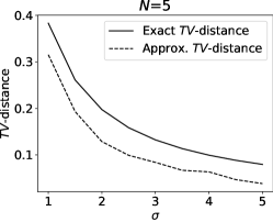
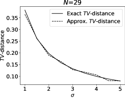
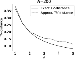
Figure 1: Too few or too many bins will lead to inaccurate estimates of hockey-stick divergences. Exact TV distance $TV(P,Q)$ and the approximated TV distance obtained using our method, when $k=5000$ and $d=1000$. Left: $N=5$ (too few bins), Center: the bin width $h_{k}$ set using Eq. (4.2) giving $N=29$ (optimal number of bins), Right: $N=200$ (too many bins).

5 Approximating DP Guarantees Using TV Distance

5.1 Approximation of $\varepsilon$ Using Any Hockey-Stick Divergence

We could in principle use any hockey-stick divergence to estimate the privacy profile of a mechanism $\mathcal{M}$ in case we can parameterize the privacy profile with a single real-valued parameter in a way that the privacy guarantees depend monotonically on that parameter. Consider, for example, the noise level $\sigma$ for the Gaussian mechanism with sensitivity 1, where finding the $\delta$-value for any $\varepsilon\in\mathbb{R}$ will also give a unique value for $\sigma$. This kind of single-parameter dependence serves as a good heuristics for analyzing DP-SGD trained models, as the privacy profiles for large compositions are commonly very close to those of a Gaussian mechanism with a given noise scale (Dong et al.,, 2022).

Thus, given an estimate of any hockey-stick divergence between the frequency estimates $\widehat{P}$ and $\widehat{Q}$ for an DP-SGD trained model, we get an estimate of the whole privacy profile and in particular get an estimate of an $\varepsilon$-value for a fixed $\delta$-value. Figure 2 illustrates this by showing the relationship between the TV distances and $\varepsilon$-values for a fixed $\delta>0$ for the Gaussian mechanism, obtained by varying the noise parameter $\sigma$. I.e., the parameter $\sigma$ is first numerically determined using the TV distance and the analytical expression of Eq. 4.3, and then the $\varepsilon$-value is numerically determined using the analytical expression of Eq. (2.2).

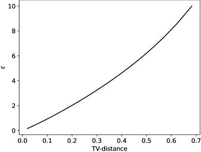
Figure 2: Relationship between TV distance $TV(P,Q)$ and $\varepsilon$ when $\delta=10^{-5}$ for the Gaussian mechanism.

We next analytically show that the choice $\alpha=1$, i.e., the TV distance, in fact gives an estimator that is not far from optimal among all hockey-stick divergences for estimating the distance between two Gaussians.

5.2 Optimal Choice of $\alpha$: Total Variation Distance

In principle, we could use any $\alpha\geq 0$ to estimate the $\alpha$-divergence between the frequency estimates $\widehat{P}$ and $\widehat{Q}$ and to subsequently deduce the parameters of the underlying mechanism $\mathcal{M}$. However, experiments indicate that the choice $\alpha=1$ is generally not far from optimum for this procedure. This is analytically explained by the following example.

Consider two one-dimensional Gaussians $P_{\sigma}\sim\mathcal{N}(0,\sigma^{2})$ and $Q_{\sigma}\sim\mathcal{N}(1,\sigma^{2})$. We first rigorously show that there is a one-to-one relationship between the hockey-stick divergence values and $\sigma$, i.e., that the hockey-stick divergence $H_{\alpha}(P_{\sigma}||Q_{\sigma})$ is an invertible function of $\sigma$ for all $\sigma\in(0,\infty)$ for all $\alpha>0$.

Lemma 1.

Let $\alpha>0$. The hockey-stick divergence $H_{\alpha}\big{(}P_{\sigma}||Q_{\sigma}\big{)}$ as a function of $\sigma$ is invertible for all $\sigma>0$.

Denote $F_{\alpha}(\sigma):=H_{\alpha}(P_{\sigma}||Q_{\sigma})$. To find a robust estimator, we would like to find an order $\alpha>0$ such that the $\sigma$-value that we obtain using the numerical approach would be least sensitive to errors in the evaluated $\alpha$-divergence. If we have an error $\approx\Delta H$ in the estimated $\alpha$-divergence, we would approximately have an error $\Delta\sigma=\left|\frac{\hskip 1.0pt{\rm d}\hskip 0.5pt}{\hskip 1.0pt{\rm d}\hskip 0.5ptH}\,F^{-1}_{\alpha}(H)\right|\cdot\Delta H$ in the estimated $\sigma$-value. Thus, we want to solve

$$\mathrm{argmin}_{\alpha>0}\,\left|\frac{\hskip 1.0pt{\rm d}\hskip 0.5pt}{\hskip 1.0pt{\rm d}\hskip 0.5ptH}\,F^{-1}_{\alpha}(H)\right|.$$

By the inverse function rule, if $H=F_{\alpha}(\sigma)$, we have that

$$\mathrm{argmin}_{\alpha>0}\,\left|\frac{\hskip 1.0pt{\rm d}\hskip 0.5pt}{\hskip 1.0pt{\rm d}\hskip 0.5ptH}\,F^{-1}_{\alpha}(H)\right|=\mathrm{argmin}_{\alpha>0}\,\left|\frac{1}{F_{\alpha}^{\prime}(\sigma)}\right|=\mathrm{argmax}_{\alpha>0}\,\left|F_{\alpha}^{\prime}(\sigma)\right|$$ (5.1)

Using the relation (5.1), we can show that the optimal hockey-stick divergence estimator is always near $\alpha=1$ which corresponds to the TV distance.

Lemma 2.

For any $\sigma>1$, as a function of $\alpha$, $\left|F_{\alpha}^{\prime}(\sigma)\right|$ has its maximum on the interval $[1,{\rm e}\hskip 1.0pt^{\frac{1}{2\sigma}}]$.

Figure 3 illustrates numerically that the optimal $\alpha$ is not far from 1 for different values of $\sigma$.

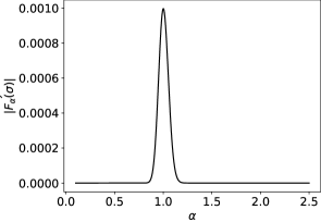
Figure 3: The value of $\left|F_{\alpha}^{\prime}(\sigma)\right|$ as a function of $\alpha$, when $\sigma=2$ (left) and $\sigma=20$ (right). We see that the optimal value is not far from $\alpha=1$, indicating that the choice $\alpha=1$ gives an estimate of $\sigma$ that is robust to errors.

6 Algorithm for Auditing the DP-Guarantees

The pseudocode for our $(\varepsilon,\delta)$-DP auditing method derived in Sections 3, 4 and 5 is given in Alg. 1. Notice that in Alg. 1, in order to find a suitable bin width $h$, we estimate the standard deviation of the score values using the auditing training data only. This is motivated by the experimental observation that the variances of the score values for auditing training and test sets are similar.

Algorithm 1 Estimation of $(\varepsilon,\delta)$-DP parameters Using Histogram Density Estimation

  Input: score function $S\,:\,\Theta\times X\rightarrow\mathbb{R}$, auditing dataset $A$, DP parameter $\delta\in(0,1)$.

  Sample $A_{\mathrm{train}}\subset A$ such that $\left|A_{\mathrm{train}}\right|=\left|A\right|/2$. Set $A_{\mathrm{test}}=A\setminus A_{\mathrm{train}}$ and $k=\left|A_{\mathrm{train}}\right|$.

  Train the model $\theta=\mathcal{M}(A_{\mathrm{train}})$ (possibly use additional training data).

  Estimate the standard deviation $\widehat{\sigma}$ of the set of score values $\{S(\theta,x)\,:\,x\in A_{\mathrm{train}}\}$.

  Set the bin width $h=3.5\cdot k^{-1/3}\widehat{\sigma}$.

  Set $a,b\in\mathbb{R}$, both multiplicatives of $h$, s.t. $S(\theta,x)\in[a,b]$ for all $x\in A$.

  Divide the interval $[a,b]$ into $N=\tfrac{b-a}{h}$ disjoint bins, each of width $h$. I.e., for $j\in[N]$,

$$\textrm{Bin}_{j}=[a+(j-1)\cdot h,a+j\cdot h].$$

Estimate the probabilities $p_{j}$ and $q_{j}$, $j\in[N]$, by the relative frequencies of hitting bin $j$ as

$$p_{j}\leftarrow\frac{\#\{x\in A_{\mathrm{train}}\,:\,S(\theta,x)\in B_{j}\}}{\left|A_{\mathrm{train}}\right|},\quad\quad\quad q_{j}\leftarrow\frac{\#\{x\in A_{\mathrm{test}}\,:\,S(\theta,x)\in B_{j}\}}{\left|A_{\mathrm{test}}\right|}$$

giving the discrete distributions $\widehat{P}$ and $\widehat{Q}$.

  Compute the TV distance $TV(\widehat{P},\widehat{Q})$ and find $\sigma>0$ such that

$$TV\big{(}\mathcal{N}(0,\sigma^{2})||\mathcal{N}(1,\sigma^{2})\big{)}=TV(\widehat{P},\widehat{Q}).$$

Find $\varepsilon>0$ such that

$$H_{{\rm e}\hskip 1.0pt^{\varepsilon}}\big{(}\mathcal{N}(0,\sigma^{2})||\mathcal{N}(1,\sigma^{2})\big{)}=\delta.$$

$\mathbf{RETURN}$ $\varepsilon$.

7 Experiments

We consider a one hidden-layer feedforward network for MNIST (LeCun et al.,, 1998) classification, with hidder-layer width 200. We also consider the CIFAR-10 (Krizhevsky and Hinton,, 2009) classification for which we use a Resnet20 pre-trained on CIFAR-100 (Krizhevsky and Hinton,, 2009) dataset so that only the last fully connected layer is trained. We minimize the cross-entropy loss for all models, and all models are trained using the Adam optimizer (Kingma and Ba,, 2014) with the default initial learning rate 0.001. To compute the theoretical $\varepsilon$-upper bounds, we use the PRV accountant of the Opacus library (Yousefpour et al.,, 2021). We use as the score function the cros-entropy loss between the initial model and the final model, i.e., $S(\theta,x)=\ell(\theta_{0},x)-\ell(\theta_{\mathrm{end}},x)$. In Appendix Fig 6 we illustrate the effect of using for auditing a different loss function than for the training.

We consider as the baseline auditing method the method by Steinke et al., (2023) and we use the implementation given in their supplementary material. The method randomly selects the auditing training set $A_{\mathrm{train}}$ from the total auditing set $A$, and based on the ordering of the loss function values, counts the number of ’correct guesses’ for the score function values. Assuming that the total number of auditing samples is even and that none of the values equals the median of all scores, the number of correct guesses equals

$$\left|\{x\in A_{\mathrm{train}}\,:\,S(\theta,x)<m\}\right|+\left|\{x\in A_{\mathrm{test}}\,:\,S(\theta,x)>m\}\right|,$$

where $m$ is the median of the score function values for the whole auditing set $A$.

We measure the $\varepsilon$-lower bound estimates both for models trained with and without DP (left and right figures of Fig. 4 and 5, respectively). We use 2000 randomly drawn auditing samples. We vary the total number of training samples, i.e., we augment the set of 1000 auditing training samples $A_{\mathrm{train}}$ with random training samples from the original dataset. In all training runs we train with batch size 100 and train for 100 epochs, and when using DP we use the clipping constant $C=0.1$ and vary the noise parameter $\sigma$ such that $\sigma\in\{0.4,0.6,\ldots,2.2\}$ when $\left|A_{\mathrm{train}}\right|=1000$, and for larger values of $\left|A_{\mathrm{train}}\right|$ we scale down the $\sigma$-values such that approximately equal $\varepsilon$-upper bounds are obtained. The results of Fig. 4 and Fig. 5 are averaged over 10 trials and the error bars on both sides of the mean values depict 1.96 times the standard error, giving the asymptotic 95% coverage. As Figures 4 and 5 show, our auditing method gives considerably more accurate $\varepsilon$-estimates than the baseline method in all experiments.

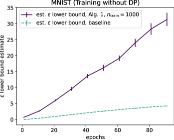
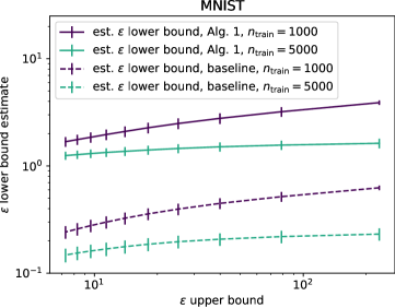
Figure 4: Training a single hidden-layer feedforward network for MNIST. The total number of training samples $n_{\mathrm{train}}$ varies. Left: the growth of $\varepsilon$-estimates along training when the model is trained using SGD. Right: the $\varepsilon$-estimates given by Alg. 1 after 100 epochs of training for different theoretical $\varepsilon$-values.

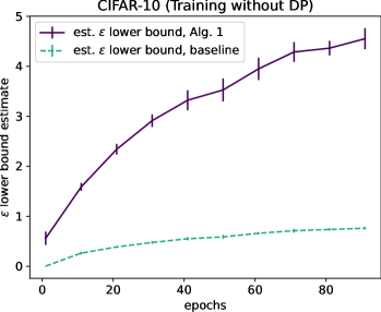
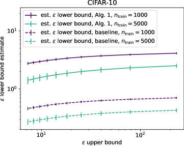
Figure 5: Fine-tuning the last layer of a pre-trained Resnet-20 for CIFAR-10. The number of training samples $n_{\mathrm{train}}$ varies. Left: the growth of $\varepsilon$-estimates along training when the model is trained using SGD. Right: the $\varepsilon$-estimates after 100 epochs of training for different theoretical $\varepsilon$-values.

8 Conclusions

We have proposed a simple and practical technique to compute empirical estimates of DP privacy guarantees in an ML model training scenario using a hold-out dataset. We have shown that our method can be seen as a generalization of existing auditing methods based on threshold membership inference attacks. The established connection also explains why our proposed method commonly gives larger $\varepsilon$-estimates than existing methods suitable for the black-box scenario. One limitation of our method is that the reported $\varepsilon$-estimates are heuristic and we do not provide confidence intervals for them. For future work, it will be interesting to find conditions under which we can circumvent the assumption of the independence of the auditing score values and possibly give confidence intervals for $\varepsilon$-lower bounds.

Appendix A Proof of Lemma 1

Lemma 1.

Let $A$ be the auditing set, $D\subset A$ the auditing training set and $A\subset D$ the auditing test set. Consider the distributions $P$ and $Q$ as defined in Eq. (3.4) obtained with 2-bin histograms defined by a threshold $\tau\in\mathbb{R}$. Suppose the underlying mechanism $\mathcal{M}$ is $(\varepsilon,\delta)$-DP for some $\varepsilon\geq 0$ and $\delta\in[0,1]$. Then,

$$\max\{H_{{\rm e}\hskip 1.0pt^{\varepsilon}}\big{(}P||Q\big{)},H_{{\rm e}\hskip 1.0pt^{\varepsilon}}\big{(}Q||P\big{)}\}=\delta,$$

where

$$\varepsilon=\max\left\{\log\frac{\mathrm{TPR}-\delta}{\mathrm{FPR}},\log\frac{\mathrm{TNR}-\delta}{\mathrm{FNR}}\right\}.$$

and $\mathrm{TPR}$ and $\mathrm{FPR}$ are as defined in Eq. (3.1) and $\mathrm{FNR}=1-\mathrm{TPR}$ and $\mathrm{TNR}=1-\mathrm{FPR}$.

Proof.

We have that $P$ and $Q$ are now discrete distributions with binary values, such that $P=(p_{1},p_{2})$, where $p_{1}=\mathrm{TPR}$, $p_{2}=\mathrm{FNR}$ and $Q=(q_{1},q_{2})$, where $q_{1}=\mathrm{FPR}$, $q_{2}=\mathrm{TNR}$. Assuming $p_{1}\geq q_{1}$, i.e., $q_{2}\geq p_{2}$, we have that

$$H_{{\rm e}\hskip 1.0pt^{\varepsilon}}\big{(}P||Q\big{)}=[p_{1}-{\rm e}\hskip 1.0pt^{\varepsilon}q_{1}]_{+}+[p_{2}-{\rm e}\hskip 1.0pt^{\varepsilon}q_{2}]_{+}=p_{1}-{\rm e}\hskip 1.0pt^{\varepsilon}q_{1}$$ (A.1)

and

$$H_{{\rm e}\hskip 1.0pt^{\varepsilon}}\big{(}Q||P\big{)}=[q_{1}-{\rm e}\hskip 1.0pt^{\varepsilon}p_{1}]_{+}+[q_{2}-{\rm e}\hskip 1.0pt^{\varepsilon}p_{2}]_{+}=q_{2}-{\rm e}\hskip 1.0pt^{\varepsilon}p_{2}.$$ (A.2)

Setting Eq. (A.1) and (A.2) equal to $\delta$ gives $\varepsilon=\frac{p_{1}-\delta}{q_{1}}$ and $\varepsilon=\frac{q_{2}-\delta}{p_{2}}$, respectively. Taking maximum of $H_{{\rm e}\hskip 1.0pt^{\varepsilon}}\big{(}P||Q\big{)}$ and $H_{{\rm e}\hskip 1.0pt^{\varepsilon}}\big{(}Q||P\big{)}$ for $\delta$ is equivalent to taking the maximum of $\frac{p_{1}-\delta}{q_{1}}$ and $\frac{p_{1}-\delta}{q_{1}}$ for $\varepsilon$. ∎

Appendix B Proof of Theorem 2

Theorem 1.

Let $A\subset X^{n}$ where $|A|$ is even, denote the total auditing set, and suppose the mechanism $\mathcal{M}$ is $(\varepsilon,\delta)$-DP. Denote

$$\widetilde{P}=S(\theta,x),\quad\textrm{where}\quad\theta\sim\mathcal{M}(D),\,D\sim\mathrm{Subsample}(A),\,x\sim D$$

and

$$\widetilde{Q}=S(\theta,x),\quad\textrm{where}\quad\theta\sim\mathcal{M}(D),\,D\sim\mathrm{Subsample}(A),\,x\sim A\setminus D,$$

where $\mathrm{Subsample}(A)$ randomly samples half of the set $A$ without replacement. Then,

$$\max\left\{H_{{\rm e}\hskip 1.0pt^{\varepsilon}}\big{(}\widetilde{P}||\widetilde{Q}\big{)},H_{{\rm e}\hskip 1.0pt^{\varepsilon}}\big{(}\widetilde{Q}||\widetilde{P}\big{)}\right\}\leq\delta.$$

Proof.

Denote $D\sim A$ short for $D\sim\mathrm{Subsample}(A)$ and $x\sim D$ short for $x\sim\mathrm{Uniform}(D)$. We have for all measurable $E\subset\mathbb{R}$:

$$\mathbb{P}\big{(}\widetilde{P}\in E\big{)}= \mathbb{P}_{D\sim A,x\sim D}\big{(}S(\mathcal{M}(D),x)\in E\big{)}$$ (B.1)

$$= \sum_{D\subset A}\sum_{x\in D}\mathbb{P}\big{(}\mathrm{Subsample}(A)=D\big{)}\cdot\mathbb{P}\big{(}\mathrm{Uniform}(D)=x\big{)}\cdot\mathbb{P}\big{(}S(\mathcal{M}(D),x)\in E\big{)}$$

$$= \sum_{D\subset A}\sum_{x\in D}\mathbb{P}\big{(}\mathrm{Subsample}(A)=D\big{)}\cdot\mathbb{P}\big{(}\mathrm{Uniform}(D)=x\big{)}\cdot$$

$$\quad\quad\left(\sum_{x^{\prime}\in A\setminus D}\mathbb{P}\big{(}\mathrm{Uniform}(A\setminus D)=x^{\prime}\big{)}\right)\cdot\mathbb{P}(S(\mathcal{M}(D),x)\in E)$$

$$\leq \sum_{D\subset A}\sum_{x\in D}\mathbb{P}\big{(}\mathrm{Subsample}(A)=D\big{)}\cdot\mathbb{P}\big{(}\mathrm{Uniform}(D)=x\big{)}\cdot$$

$$\quad\quad\left(\sum_{x^{\prime}\in A\setminus D}\mathbb{P}\big{(}\mathrm{Uniform}(A\setminus D)=x^{\prime}\big{)}\big{(}{\rm e}\hskip 1.0pt^{\varepsilon}\mathbb{P}(S(\mathcal{M}(D\setminus\{x\}\cup\{x^{\prime}\}),x)\in E)+\delta\big{)}\right)$$

$$= \delta+{\rm e}\hskip 1.0pt^{\varepsilon}\sum_{D\subset A}\sum_{x\in D}\sum_{x^{\prime}\in A\setminus D}\mathbb{P}\big{(}\mathrm{Subsample}(A)=D\big{)}\cdot\mathbb{P}\big{(}\mathrm{Uniform}(D)=x\big{)}\cdot$$

$$\quad\quad\mathbb{P}\big{(}\mathrm{Uniform}(A\setminus D)=x^{\prime}\big{)}\cdot\mathbb{P}\big{(}S(\mathcal{M}(D\setminus\{x\}\cup\{x^{\prime}\}),x)\in E\big{)}$$

$$= \delta+{\rm e}\hskip 1.0pt^{\varepsilon}\sum_{D\subset A}\sum_{x\in D}\sum_{x^{\prime}\in A\setminus D}\frac{1}{{\left|A\right|\choose\left|D\right|}}\cdot\frac{1}{\left|D\right|}\cdot\frac{1}{\left|D\right|}\cdot\mathbb{P}\big{(}S(\mathcal{M}(D\setminus\{x\}\cup\{x^{\prime}\}),x)\in E\big{)}$$

$$= \delta+{\rm e}\hskip 1.0pt^{\varepsilon}\frac{1}{{\left|A\right|\choose\left|D\right|}}\cdot\frac{1}{\left|D\right|}\cdot\frac{1}{\left|D\right|}\cdot\sum_{D\subset A}\sum_{x\in D}\sum_{x^{\prime}\in A\setminus D}\mathbb{P}\big{(}S(\mathcal{M}(D\setminus\{x\}\cup\{x^{\prime}\}),x)\in E\big{)}$$

where the inequality follows from the fact that $\mathcal{M}$ is $(\varepsilon,\delta)$-DP under substitute neighborhood relation.

We see that for any triplet $(D,x,x^{\prime})$, where $D\subset A$, $\left|D\right|=\left|A\right|/2$, $x\in D$ and $x^{\prime}\in A\setminus D$, there exist exactly $\left|D\right|$ pairs $(\widetilde{D},x^{\prime})$, where $\widetilde{D}\subset A$, $\left|\widetilde{D}\right|=\left|A\right|/2$ and $x^{\prime}\in A\setminus\widetilde{D}$, such that

$$(\widetilde{D}\setminus\{x\}\cup\{x^{\prime}\},x)=(D\setminus\{x\}\cup\{x^{\prime}\},x).$$

On the other hand, for any $D\subset A$, $\left|D\right|=\left|A\right|/2$ and $x\in A\setminus D$, there exist $\widetilde{D}\subset A$, $\left|\widetilde{D}\right|=\left|A\right|/2$ and $x^{\prime}\in A\setminus\widetilde{D}$ such that

$$(\widetilde{D}\setminus\{x\}\cup\{x^{\prime}\},x)=(D\setminus\{x\}\cup\{x^{\prime}\},x).$$

Therefore,

$$\sum_{D\subset A}\sum_{x\in D}\sum_{x^{\prime}\in A\setminus D}\mathbb{P}\big{(}S(\mathcal{M}(D\setminus\{x\}\cup\{x^{\prime}\}),x)\in E\big{)}=\left|D\right|\cdot\sum_{D\subset A}\sum_{x\in A\setminus D}\mathbb{P}\big{(}S(\mathcal{M}(D),x)\in E\big{)}.$$ (B.2)

Together from (B.3) and (B.2) it follows that

$$\mathbb{P}\big{(}\widetilde{P}\in E\big{)}= \mathbb{P}_{D\sim A,x\sim D}\big{(}S(\mathcal{M}(D),x)\in E\big{)}$$ (B.3)

$$\leq \delta+{\rm e}\hskip 1.0pt^{\varepsilon}\frac{1}{{\left|A\right|\choose\left|D\right|}}\cdot\frac{1}{\left|D\right|}\cdot\sum_{D\subset A}\sum_{x\in A\setminus D}\mathbb{P}\big{(}S(\mathcal{M}(D),x)\in E\big{)}$$

$$= \delta+{\rm e}\hskip 1.0pt^{\varepsilon}\sum_{D\subset A}\sum_{x\in A\setminus D}\mathbb{P}\big{(}\mathrm{Subsample}(A)=D\big{)}\cdot\mathbb{P}\big{(}\mathrm{Uniform}(A\setminus D)=x\big{)}\cdot\mathbb{P}\big{(}S(\mathcal{M}(D),x)\in E\big{)}$$

$$= \delta+{\rm e}\hskip 1.0pt^{\varepsilon}\mathbb{P}\big{(}\widetilde{Q}\in E\big{)}.$$

This proves that $\mathbb{P}\big{(}\widetilde{P}\in E\big{)}\leq{\rm e}\hskip 1.0pt^{\varepsilon}\mathbb{P}\big{(}\widetilde{Q}\in E\big{)}+\delta$ for any measurable $E\subset\mathbb{R}$. Notice that the only inequality above comes from the DP property of $\mathcal{M}$ and from the post-processing property of DP, when we use in Eq. (B.3) the following bound:

$$\mathbb{P}(S(\mathcal{M}(D),x)\in E)\leq{\rm e}\hskip 1.0pt^{\varepsilon}\mathbb{P}(S(\mathcal{M}(D\setminus\{x\}\cup\{x^{\prime}\}),x)\in E)+\delta.$$ (B.4)

Inverting all the steps above and instead of Eq. (B.4), using the bound

$$\mathbb{P}(S(\mathcal{M}(D\setminus\{x\}\cup\{x^{\prime}\}),x)\in E)\leq{\rm e}\hskip 1.0pt^{\varepsilon}\mathbb{P}(S(\mathcal{M}(D),x)\in E)+\delta,$$

we see that also $\mathbb{P}\big{(}\widetilde{Q}\in E\big{)}\leq{\rm e}\hskip 1.0pt^{\varepsilon}\mathbb{P}\big{(}\widetilde{P}\in E\big{)}+\delta$ for any measurable $E\subset\mathbb{R}$ and therefore

$$\max\left\{H_{{\rm e}\hskip 1.0pt^{\varepsilon}}\big{(}\widetilde{P}||\widetilde{Q}\big{)},H_{{\rm e}\hskip 1.0pt^{\varepsilon}}\big{(}\widetilde{Q}||\widetilde{P}\big{)}\right\}\leq\delta.$$

∎

Appendix C Proof of Theorem 3

We first state some auxiliary results needed for the proof.

Recall first the following lemma from (Andrew et al.,, 2024) which essentially says that maximal cosine similarity between $n$ random unit vectors goes to zero in distribution as the dimension $d$ grows.

Lemma 1 (Andrew et al., 2024).

For $d\in\mathbb{N}$, $d\geq 2$, let $c$ be sampled uniformly from $\mathbb{S}^{d-1}$, and let $\rho=\langle c^{T}v\rangle\in[-1,1]$ for some arbitrary $v\in\mathbb{S}^{d-1}$. Then, for all $\lambda\in\mathbb{R}$,

$$\lim_{d\rightarrow\infty}\mathbb{P}(\rho\leq\lambda/\sqrt{d})=\mathbb{P}_{Z\sim\mathcal{N}(0,1)}(Z\leq\lambda).$$

Moreover, the cosine angles between $n$ randomly chosen vectors from the unit sphere are independent random variables.

Lemma 2 (Cai et al., 2013, Lemma 6.1,).

Let $x_{1},\ldots,x_{n}$ be independently chosen random vectors from the unit sphere $\mathbb{S}^{d-1}$. Denote $\rho_{ij}$ the cosine angle between the vectors $x_{i}$ and $x_{j}$. Then, for $1\leq i\leq j\leq n$, $\rho_{ij}$’s are mutually independent.

Using Lemma 2, we directly get from Lemma 1 the following corollary.

Lemma 3.

Let $x_{1},\ldots,x_{n}$ be independently uniformly chosen random vectors from the unit sphere $\mathbb{S}^{d-1}$. Denote $\rho_{ij}$ the cosine angle between the vectors $x_{i}$ and $x_{j}$. Then, for $1\leq i\leq j\leq n$, $\rho_{ij}$’s are mutually independent. Denote $\rho_{\max}:=\max_{i,j}\rho_{ij}$. Then, Then, for all $\lambda\in\mathbb{R}$,

$$\lim_{d\rightarrow\infty}\mathbb{P}(\rho_{\max}\leq\lambda/\sqrt{d})\leq\mathbb{P}_{Z\sim\mathcal{N}(0,1)}(Z\leq\lambda)^{n^{2}}.$$

Moreover, $\rho_{\max}$ converges in probability to 0 as $d\rightarrow\infty$.

Theorem 4.

Suppose the dataset $X=\{x_{1},\ldots,x_{n}\}$, where $x_{i}$’s are i.i.d. uniformly sampled from the unit sphere $\mathbb{S}^{d-1}$. Suppose $\mathcal{M}$ is the DP mean estimation mechanism, i.e.,

$$\mathcal{M}(X)=\sum_{x\in X}x+Z,\quad Z\sim\mathcal{N}(0,\sigma^{2}),$$

where $\sigma>0$ is chosen such that $\mathcal{M}$ is tightly $(\varepsilon,\delta)$-DP. Let $P$ and $Q$ be as defined in Eq. (3.4) using a random draw $D\subset A$. Then, for any fixed $n\in\mathbb{N}$ and for any $\tau>0$,

$$\mathbb{P}\left(\left|H_{{\rm e}\hskip 1.0pt^{\varepsilon}}\big{(}P||Q\big{)}-\delta\right|>\tau\right)\rightarrow 0\quad\textrm{as}\quad d\rightarrow\infty.$$

Proof.

We see that for any $z\in D$,

$$S\big{(}z,\mathcal{M}(D)\big{)}\sim z^{T}\left(\sum\limits_{x\in D}x+\mathcal{N}(0,\sigma^{2}I_{d})\right)\sim 1+\sum\limits_{x\in D,\,x\neq z}z^{T}x+\mathcal{N}(0,\sigma^{2}),$$

and for any $z\in A\setminus D$,

$$S\big{(}z,\mathcal{M}(D)\big{)}\sim z^{T}\left(\sum\limits_{x\in D}x+\mathcal{N}(0,\sigma^{2}I_{d})\right)\sim\sum\limits_{x\in D}z^{T}x+\mathcal{N}(0,\sigma^{2}).$$

For any ordering $D=\{z_{1},\ldots,z_{k}\}$, $A\setminus D=\{\widehat{z}_{1},\ldots,\widehat{z}_{k}\}$, using the joint convexity of the hockey-stick divergence we have that

$$H_{{\rm e}\hskip 1.0pt^{\varepsilon}}\big{(}P||Q\big{)}\leq\frac{1}{k}\sum_{i=1}^{k}H_{{\rm e}\hskip 1.0pt^{\varepsilon}}\bigg{(}1+\sum\nolimits_{x\in D,\,x\neq z_{i}}z_{i}^{T}x+\mathcal{N}(0,\sigma^{2})||\sum\nolimits_{x\in D}\widehat{z}_{i}^{T}x+\mathcal{N}(0,\sigma^{2})\bigg{)}.$$

Under the assumption that the samples are uniformly sampled from the unit sphere $\mathbb{S}^{d-1}$, by Lemma 3, we have that for all $z_{i}\in D$,

$$\left|\sum\nolimits_{x\in D,\,x\neq z_{i}}z_{i}^{T}x\right|\leq k\cdot\rho_{\max}$$

and for all $\widehat{z}_{i}\in A\setminus D$,

$$\left|\sum\nolimits_{x\in D}\widehat{z}_{i}^{T}x\right|\leq k\cdot\rho_{\max},$$

where $\rho_{\max}$ converges in probability to 0 as $d\rightarrow\infty$.

As the hockey-stick divergence of the Gaussian mechanism is a continuous function of the sensitivity, we have that for all $i\in[k]$,

$$H_{{\rm e}\hskip 1.0pt^{\varepsilon}}\bigg{(}1+\sum\nolimits_{x\in D,\,x\neq z_{i}}z_{i}^{T}x+\mathcal{N}(0,\sigma^{2})||\sum\nolimits_{x\in D}\widehat{z}_{i}^{T}x+\mathcal{N}(0,\sigma^{2})\bigg{)}\rightarrow H_{{\rm e}\hskip 1.0pt^{\varepsilon}}\bigg{(}1+\mathcal{N}(0,\sigma^{2})||\mathcal{N}(0,\sigma^{2})\bigg{)}$$

in probability as $d\rightarrow\infty$ which shows the claim.

∎

Appendix D Proof of Lemma 4

Theorem 1.

Let $\tau>0$. Suppose that with probability $1-\tau$ w.r.t. to the randomness of sampling $D\subset A$, for some $\widehat{\delta}>0$, for all measurable $E\subset\mathbb{R}$,

$$\mathbb{P}_{x^{\prime}\sim A\setminus D,x\sim D}\big{(}S(\mathcal{M}(D\setminus\{x\}\cup\{x^{\prime}\}),x)\in E\big{)}-\mathbb{P}_{x\sim A\setminus D}\big{(}S(\mathcal{M}(D),x)\in E\big{)}\leq\widehat{\delta}$$

and suppose $\mathcal{M}$ is $(\varepsilon,\delta)$-DP for some $\varepsilon\in\mathbb{R}$. Then, for $P$ and $Q$ as defined in Eq. (3.4), we have with probability $1-\tau$,

$$H_{{\rm e}\hskip 1.0pt^{\varepsilon}}\big{(}P||Q\big{)}\leq\delta+{\rm e}\hskip 1.0pt^{\varepsilon}\cdot\widehat{\delta}.$$ (D.1)

Suppose that with probability $1-\tau$ w.r.t. to the randomness of sampling $D\subset A$, for some $\widehat{\delta}>0$, for all measurable $E\subset\mathbb{R}$,

$$\mathbb{P}_{x\sim A\setminus D,x^{\prime}\sim D}\big{(}S(\mathcal{M}(D\setminus\{x^{\prime}\}\cup\{x\}),x)\in E\big{)}-\mathbb{P}_{x\sim D}\big{(}S(\mathcal{M}(D),x)\in E\big{)}\leq\widehat{\delta}$$

and suppose $\mathcal{M}$ is $(\varepsilon,\delta)$-DP for some $\varepsilon\in\mathbb{R}$. Then, for $P$ and $Q$ as defined in Eq. (3.4), we have with probability $1-\tau$,

$$H_{{\rm e}\hskip 1.0pt^{\varepsilon}}\big{(}Q||P\big{)}\leq\delta+{\rm e}\hskip 1.0pt^{\varepsilon}\cdot\widehat{\delta}.$$ (D.2)

Proof.

For any measurable $E\subset\mathbb{R}$:

$$\mathbb{P}\big{(}P\in E\big{)} =\mathbb{P}_{D\sim A,x\sim D}\big{(}S(\mathcal{M}(D),x)\in E\big{)}$$

$$\leq{\rm e}\hskip 1.0pt^{\varepsilon}\cdot\mathbb{P}_{D\sim A,x\sim D,x^{\prime}\sim A\setminus D}\big{(}S(\mathcal{M}(D\setminus\{x\}\cup\{x^{\prime}\}),x)\in E\big{)}+\delta$$

$$={\rm e}\hskip 1.0pt^{\varepsilon}\cdot\left(\mathbb{P}_{D\sim A,x\sim D,x^{\prime}\sim A\setminus D}\big{(}S(\mathcal{M}(D\setminus\{x\}\cup\{x^{\prime}\}),x)\in E\big{)}-\mathbb{P}_{x\sim A\setminus D}\big{(}S(\mathcal{M}(D),x)\in E\big{)}\right)$$

$$\quad+{\rm e}\hskip 1.0pt^{\varepsilon}\cdot\mathbb{P}_{x\sim A\setminus D}\big{(}S(\mathcal{M}(D),x)\in E\big{)}+\delta$$

which shows the inequality (D.1). Showing the inequality (D.2) goes analogously.

∎

Appendix E Proof of Theorem 1

Theorem 1.

Let $P$ and $Q$ be one-dimensional probability distributions. Consider drawing $k$ samples both from $P$ and $Q$, giving density estimators $P_{k}=(\widehat{P}_{1},\ldots,\widehat{P}_{N})$ and $Q_{k}=(\widehat{Q}_{1},\ldots,\widehat{Q}_{N})$, respectively. Let the bin width be

$$h_{k}=\left(\frac{12}{\int P^{\prime}(x)^{2}\,\hskip 1.0pt{\rm d}\hskip 0.5ptx+\int Q^{\prime}(x)^{2}\,\hskip 1.0pt{\rm d}\hskip 0.5ptx}\right)^{\frac{1}{3}}k^{-\frac{1}{3}}$$ (E.1)

Then, for any $\alpha\geq 0$, the numerical hockey-stick divergence $H_{\alpha}(P_{k}||Q_{k})$ convergences in expectation to $H_{\alpha}(P||Q)$ with speed $\mathcal{O}(k^{-2/3})$, i.e.,

$$\mathbb{E}\left|H_{\alpha}(P_{k}||Q_{k})-H_{\alpha}(P||Q)\right|=\mathcal{O}(k^{-2/3}),$$

where the expectation is taken over the random draws from $P$ and $Q$ for constructing $P_{k}$ and $Q_{k}$, respectively.

Proof.

Define the piece-wise continuous functions $P_{k}(x)$ and $Q_{k}(x)$. I.e., let $P_{k}(x)=\widehat{P}_{\ell}/h$, if $x\in\textrm{Bin}_{\ell}$ and similarly for $Q_{k}(x)$. To analyse the error we can use $P_{k}(x)$ and $Q_{k}(x)$ since

$$H_{\alpha}(P_{k}||Q_{k})=\sum_{\ell=1}^{N}\max\{\widehat{P}_{\ell}-\alpha\cdot\widehat{Q}_{\ell},0\}=\int\max\{P_{k}(x)-\alpha\cdot Q_{k}(x),0\}\,\hskip 1.0pt{\rm d}\hskip 0.5ptx.$$

Furthermore, we have for the expectation of the divergence $H_{\alpha}(P_{k}||Q_{k})$ (where the expectation is taken over the random draws from $P$ and $Q$) :

$$\mathbb{E}H_{\alpha}(P_{k} ||Q_{k})$$ (E.2)

$$= \mathbb{E}\int\max\{P_{k}(x)-\alpha\cdot Q_{k}(x),0\}\,\hskip 1.0pt{\rm d}\hskip 0.5ptx$$

$$= \int\mathbb{E}\max\{P_{k}(x)-\alpha\cdot Q_{k}(x),0\}\,\hskip 1.0pt{\rm d}\hskip 0.5ptx$$

$$= \int\mathbb{E}\max\{P_{k}(x)-P(x)-\alpha\cdot(Q_{k}(x)-Q(x))+P(x)-\alpha\cdot Q(x),0\}\,\hskip 1.0pt{\rm d}\hskip 0.5ptx$$

$$\leq \int\mathbb{E}\left|P_{k}(x)-P(x)\right|\,\hskip 1.0pt{\rm d}\hskip 0.5ptx+\alpha\int\mathbb{E}\left|Q_{k}(x)-Q(x)\right|\,\hskip 1.0pt{\rm d}\hskip 0.5ptx+\int\mathbb{E}\max\{P(x)-\alpha\cdot Q(x),0\}\,\hskip 1.0pt{\rm d}\hskip 0.5ptx$$

$$\leq \sqrt{\int\mathbb{E}(P_{k}(x)-P(x))^{2}\,\hskip 1.0pt{\rm d}\hskip 0.5ptx}+\alpha\sqrt{\int\mathbb{E}(Q_{k}(x)-Q(x))^{2}\,\hskip 1.0pt{\rm d}\hskip 0.5ptx}+\int\mathbb{E}\max\{P(x)-\alpha\cdot Q(x),0\}\,\hskip 1.0pt{\rm d}\hskip 0.5ptx$$

$$= \sqrt{\int\mathbb{E}(P_{k}(x)-P(x))^{2}\,\hskip 1.0pt{\rm d}\hskip 0.5ptx}+\alpha\sqrt{\int\mathbb{E}(Q_{k}(x)-Q(x))^{2}\,\hskip 1.0pt{\rm d}\hskip 0.5ptx}+\mathbb{E}H_{\alpha}(P||Q),$$

where the first inequality follows from the fact that $\max\{a+b,0\}\leq\left|a\right|+\max\{b,0\}$ for all $a,b\in\mathbb{R}$, and the second inequality follows from the Hölder inequality.

Using the inequality $\sqrt{a}+\sqrt{b}\leq\sqrt{2}\sqrt{a+b}$ which holds for any $a,b\geq 0$, we have that

$$\sqrt{\int\mathbb{E}(P_{k}(x)-P(x))^{2}\,\hskip 1.0pt{\rm d}\hskip 0.5ptx}+\sqrt{\int\mathbb{E}(Q_{k}(x)-Q(x))^{2}\,\hskip 1.0pt{\rm d}\hskip 0.5ptx}$$ (E.3)

$$\leq \sqrt{2}\sqrt{\int\mathbb{E}(P_{k}(x)-P(x))^{2}\,\hskip 1.0pt{\rm d}\hskip 0.5ptx+\int\mathbb{E}(Q_{k}(x)-Q(x))^{2}\,\hskip 1.0pt{\rm d}\hskip 0.5ptx}.$$

By the results of (Sec. 3 Scott,, 1979), we have that

$$\int\mathbb{E}(P_{k}(x)-P(x))^{2}\,\hskip 1.0pt{\rm d}\hskip 0.5ptx+\int\mathbb{E}(Q_{k}(x)-Q(x))^{2}\,\hskip 1.0pt{\rm d}\hskip 0.5ptx$$ (E.4)

$$= \frac{2}{k\cdot h}+\frac{1}{12}h^{2}\left[\int P^{\prime}(x)^{2}\,\hskip 1.0pt{\rm d}\hskip 0.5ptx+\int Q^{\prime}(x)^{2}\,\hskip 1.0pt{\rm d}\hskip 0.5ptx\right]+\mathcal{O}\left(\frac{1}{k}+h^{3}\right)$$

Minimizing the first two terms on the right-hand side of (E.4) with respect to $h$ gives the expression $h_{k}$ of Eq. (E.1) and furthermore, with this optimal choice $h_{k}$, we have that

$$\int\mathbb{E}(P_{k}(x)-P(x))^{2}\,\hskip 1.0pt{\rm d}\hskip 0.5ptx+\int\mathbb{E}(Q_{k}(x)-Q(x))^{2}\,\hskip 1.0pt{\rm d}\hskip 0.5ptx=\mathcal{O}\left(k^{-\frac{2}{3}}\right).$$

which together with inequalities (E.2) and  (E.3) shows that

$$H_{\alpha}(P_{k}||Q_{k})-H_{\alpha}(P||Q)=\mathcal{O}(k^{-\frac{1}{3}}).$$ (E.5)

Similarly, carrying out the same calculation starting from $H_{\alpha}(P||Q)$, we have

$$H_{\alpha}(P||Q) =\int\max\{P(x)-\alpha\cdot Q(x),0\}\,\hskip 1.0pt{\rm d}\hskip 0.5ptx$$

$$\leq\int\mathbb{E}\left|P_{k}(x)-P(x)\right|\,\hskip 1.0pt{\rm d}\hskip 0.5ptx+\alpha\int\mathbb{E}\left|Q_{k}(x)-Q(x)\right|\,\hskip 1.0pt{\rm d}\hskip 0.5ptx+\int\mathbb{E}\max\{P_{k}(x)-\alpha\cdot Q_{k}(x),0\}\,\hskip 1.0pt{\rm d}\hskip 0.5ptx$$

$$=\int\mathbb{E}\left|P_{k}(x)-P(x)\right|\,\hskip 1.0pt{\rm d}\hskip 0.5ptx+\alpha\int\mathbb{E}\left|Q_{k}(x)-Q(x)\right|\,\hskip 1.0pt{\rm d}\hskip 0.5ptx+\mathbb{E}H_{\alpha}(P_{k}||Q_{k})$$

which eventually gives

$$H_{\alpha}(P||Q)-H_{\alpha}(P_{k}||Q_{k})=\mathcal{O}(k^{-\frac{1}{3}})$$

which together with Eq. (E.5) shows the claim. ∎

Appendix F Proof of Lemma 1

Lemma 1.

The hockey-stick divergence $H_{\alpha}(P_{\sigma}||Q_{\sigma})$ as a function of $\sigma$ is invertible for all $\sigma\in(0,\infty)$.

Proof.

From Eq. (2.2) we know that

$$F_{\alpha}^{\prime}(\sigma)=\left(-\log\alpha-\frac{1}{2\sigma^{2}}\right)\cdot f\left(-\sigma\log\alpha+\frac{1}{2\sigma}\right)-\alpha\cdot\left(-\log\alpha+\frac{1}{2\sigma^{2}}\right)\cdot f\left(-\sigma\log\alpha-\frac{1}{2\sigma}\right),$$ (F.1)

where $f$ denotes the density function of the standard univariate Gaussian distribution. We see from Eq. (F.1) that for $\alpha=1$, the value of $F_{\alpha}^{\prime}(\sigma)$ is strictly negative for all $\sigma>0$. We also know that if a post-processing function reduces the total variation distance, it reduces then all other hockey-stick divergences, since the contraction constant of all hockey-stick divergences is bounded by the contraction constant of the total variation distance. This follows from the fact that for any Markov kernel $\mathrm{K}$, and for any pair distributions $(P,Q)$ and for any $f$-divergence $D_{f}(\cdot||\cdot)$, we have that $D_{f}(P\mathrm{K}||Q\mathrm{K})\leq\mathrm{TV}(P,Q)\cdot D_{f}(P||Q)$ (see, e.g., Lemma 1 and Thm. 1, Asoodeh et al.,, 2021). Therefore, $F_{\alpha}^{\prime}(\sigma)$ is strictly negative for all $\alpha\geq 0$. ∎

Appendix G Proof of Lemma 2

Lemma 1.

For any $\sigma>1$, as a function of $\alpha$, $\left|F_{\alpha}^{\prime}(\sigma)\right|$ has its maximum on the interval $[1,{\rm e}\hskip 1.0pt^{\frac{1}{2\sigma}}]$.

Proof.

The proof goes by looking at the expression $\frac{\hskip 1.0pt{\rm d}\hskip 0.5pt}{\hskip 1.0pt{\rm d}\hskip 0.5pt\alpha}F_{\alpha}^{\prime}(\sigma)$. Clearly $F_{\alpha}^{\prime}(\sigma)$ is negative for all $\sigma>0$ and for all $\alpha\geq 0$. Thus $\left|F_{\alpha}^{\prime}(\sigma)\right|=-F_{\alpha}^{\prime}(\sigma)$.

Using the expression (F.1), a lengthy calculation shows that

$$\frac{\hskip 1.0pt{\rm d}\hskip 0.5pt}{\hskip 1.0pt{\rm d}\hskip 0.5pt\alpha}F_{\alpha}^{\prime}(\sigma)= \frac{1}{\sqrt{2\pi}}{\rm e}\hskip 1.0pt^{-\frac{1}{2}(\frac{1}{2\sigma}+\log\alpha)^{2}}\left(\left(\frac{1}{2\sigma}+\log\alpha\right)\left(\frac{1}{2\sigma^{2}}-\log\alpha\right)-\left(\frac{1}{2\sigma^{2}}-\log\alpha\right)+1\right)$$ (G.1)

$$+\frac{1}{\sqrt{2\pi}}{\rm e}\hskip 1.0pt^{-\frac{1}{2}(\frac{1}{2\sigma}-\log\alpha)^{2}}\left(\left(-\frac{1}{2\sigma^{2}}-\log\alpha\right)\left(\frac{1}{2\sigma}-\log\alpha\right)-\frac{1}{\alpha}\right).$$

When $\alpha=1$, i.e., $\log\alpha=0$, we find from Eq. (G.1) that

$$\frac{\hskip 1.0pt{\rm d}\hskip 0.5pt}{\hskip 1.0pt{\rm d}\hskip 0.5pt\alpha}F_{\alpha}^{\prime}(\sigma)|_{\alpha=1}=-\frac{1}{2\sqrt{2\pi}\sigma^{2}}{\rm e}\hskip 1.0pt^{-\frac{1}{8\sigma^{2}}}<0.$$

On the other hand, when $\log\alpha=\frac{1}{2\sigma}$, we see from Eq. (G.1) that

$$\frac{\hskip 1.0pt{\rm d}\hskip 0.5pt}{\hskip 1.0pt{\rm d}\hskip 0.5pt\alpha}F_{\alpha}^{\prime}(\sigma)|_{\alpha=\exp\big{(}\frac{1}{2\sigma}\big{)}} =\frac{1}{\sqrt{2\pi}}{\rm e}\hskip 1.0pt^{-\frac{1}{2\sigma^{2}}}\left(\frac{1}{\sigma}\left(\frac{1}{2\sigma^{2}}-\frac{1}{\sigma}\right)-\left(\frac{1}{2\sigma^{2}}-\frac{1}{\sigma}\right)\right)+\frac{1}{\sqrt{2\pi}}\left({\rm e}\hskip 1.0pt^{-\frac{1}{2\sigma^{2}}}-{\rm e}\hskip 1.0pt^{-\frac{1}{2\sigma}}\right)$$

$$=\frac{1}{\sqrt{2\pi}}{\rm e}\hskip 1.0pt^{-\frac{1}{2\sigma^{2}}}\left(1-\frac{1}{\sigma}\right)\left(\frac{1}{\sigma}-\frac{1}{2\sigma^{2}}\right)+\frac{1}{\sqrt{2\pi}}\left({\rm e}\hskip 1.0pt^{-\frac{1}{2\sigma^{2}}}-{\rm e}\hskip 1.0pt^{-\frac{1}{2\sigma}}\right)$$

which shows that $\frac{\hskip 1.0pt{\rm d}\hskip 0.5pt}{\hskip 1.0pt{\rm d}\hskip 0.5pt\alpha}F_{\alpha}^{\prime}(\sigma)|_{\alpha=\exp\big{(}\frac{1}{2\sigma}\big{)}}>0$ when $\sigma>1$.

Moreover, we can infer from Eq. (G.1) that $\frac{\hskip 1.0pt{\rm d}\hskip 0.5pt}{\hskip 1.0pt{\rm d}\hskip 0.5pt\alpha}F_{\alpha}^{\prime}(\sigma)$ is negative when $0\leq\alpha<1$ and positive for $\alpha>{\rm e}\hskip 1.0pt^{\frac{1}{2\sigma}}$. Thus $\frac{\hskip 1.0pt{\rm d}\hskip 0.5pt}{\hskip 1.0pt{\rm d}\hskip 0.5pt\alpha}\left|F_{\alpha}^{\prime}(\sigma)\right|=-\frac{\hskip 1.0pt{\rm d}\hskip 0.5pt}{\hskip 1.0pt{\rm d}\hskip 0.5pt\alpha}F_{\alpha}^{\prime}(\sigma)$ has its maximum on the interval $[1,{\rm e}\hskip 1.0pt^{\frac{1}{2\sigma}}]$.

∎

Appendix H Example with Different Score Function

One might intuitively think that the using the same loss function $\ell$ for the auditing as for the training will likely give the best auditing results, as the training has minimized $\ell$ for the training data and thus the distance of $P$ and $Q$ will become larger. However, we are free to use any score function $S$ to generate $P$ and $Q$ and using, e.g., some other loss function will likely show the possible overfitting as well.

Consider training of a fully connected one hidden-layer neural network for the MNIST classification problem using the MSE loss function. We carry out the auditing using as the score function the loss between the initial model and the final model, i.e., $S(\theta,x)=\ell(\theta_{0})-\ell(\theta_{\mathrm{end}})$, when $\ell$ is a) The MSE loss function, b) the cross entropy loss function.

As Fig. 6 shows, also other loss functions than the one used for training is able to detect that the DP parameters are high (true answer being ”no DP used” in this case) and most importantly, the method still give much more accurate answer than the existing baseline method by Steinke et al., (2023).

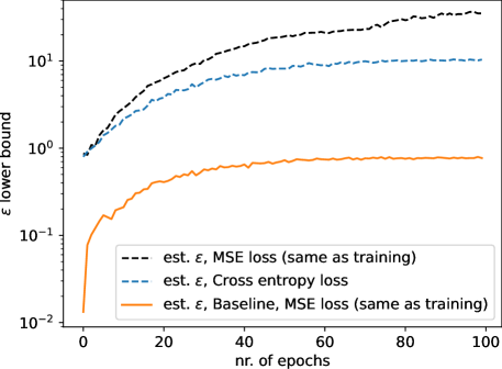
Figure 6: The model is a fully connected one hidden-layer neural network trained for the MNIST classification problem using SGD and the MSE loss function (i.e., without DP). Auditing is carried out by using MSE loss and the cross entropy loss.

Appendix I Varying the Total Number of Training Samples

Figures 7 and 8 show results with more values of $n_{\mathrm{train}}$ for the experiments of Fig. 4 and 5 of the main text.

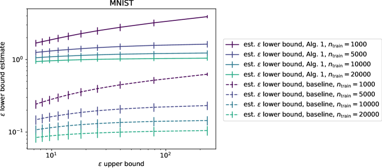
Figure 7: Training a single hidden-layer feedforward network for MNIST. The total number of training samples $n_{\mathrm{train}}$ varies. Left: the growth of $\varepsilon$-estimates along training when the model is trained using SGD. Right: the $\varepsilon$-estimates given by Alg. 1 after 100 epochs of training for different theoretical $\varepsilon$-values.

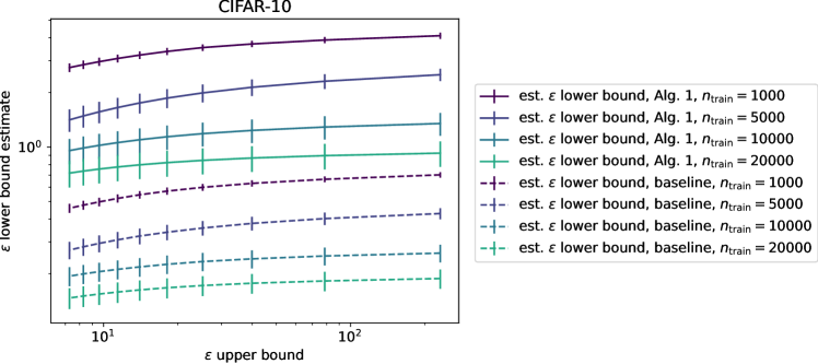
Figure 8: Fine-tuning the last layer of a pre-trained Resnet-20 for CIFAR-10. The number of training samples $n_{\mathrm{train}}$ varies. Left: the growth of $\varepsilon$-estimates along training when the model is trained using SGD. Right: the $\varepsilon$-estimates after 100 epochs of training for different theoretical $\varepsilon$-values.

References

- Abadi et al., (2016) Abadi, M., Chu, A., Goodfellow, I., McMahan, H. B., Mironov, I., Talwar, K., and Zhang, L. (2016). Deep learning with differential privacy. In Proceedings of the 2016 ACM SIGSAC Conference on Computer and Communications Security, pages 308–318.
- Andrew et al., (2024) Andrew, G., Kairouz, P., Oh, S., Oprea, A., McMahan, H. B., and Suriyakumar, V. M. (2024). One-shot empirical privacy estimation for federated learning. In The Twelfth International Conference on Learning Representations.
- Asoodeh et al., (2021) Asoodeh, S., Aliakbarpour, M., and Calmon, F. P. (2021). Local differential privacy is equivalent to contraction of an -divergence. In 2021 IEEE International Symposium on Information Theory (ISIT), pages 545–550. IEEE.
- Balle et al., (2018) Balle, B., Barthe, G., and Gaboardi, M. (2018). Privacy amplification by subsampling: Tight analyses via couplings and divergences. In Advances in Neural Information Processing Systems, volume 31.
- Balle et al., (2020) Balle, B., Barthe, G., and Gaboardi, M. (2020). Privacy profiles and amplification by subsampling. Journal of Privacy and Confidentiality, 10(1).
- Balle and Wang, (2018) Balle, B. and Wang, Y.-X. (2018). Improving the gaussian mechanism for differential privacy: Analytical calibration and optimal denoising. In International Conference on Machine Learning, pages 394–403.
- Cai et al., (2013) Cai, T., Fan, J., and Jiang, T. (2013). Distributions of angles in random packing on spheres. The Journal of Machine Learning Research, 14(1):1837–1864.
- Carlini et al., (2022) Carlini, N., Chien, S., Nasr, M., Song, S., Terzis, A., and Tramer, F. (2022). Membership inference attacks from first principles. In 2022 IEEE Symposium on Security and Privacy (SP), pages 1897–1914. IEEE.
- Carlini et al., (2019) Carlini, N., Liu, C., Erlingsson, Ú., Kos, J., and Song, D. (2019). The secret sharer: Evaluating and testing unintended memorization in neural networks. In 28th USENIX security symposium (USENIX security 19), pages 267–284.
- Dong et al., (2022) Dong, J., Roth, A., Su, W. J., et al. (2022). Gaussian differential privacy. Journal of the Royal Statistical Society Series B, 84(1):3–37.
- Dwork et al., (2006) Dwork, C., McSherry, F., Nissim, K., and Smith, A. (2006). Calibrating noise to sensitivity in private data analysis. In Proc. TCC 2006, pages 265–284.
- Gopi et al., (2021) Gopi, S., Lee, Y. T., and Wutschitz, L. (2021). Numerical composition of differential privacy. In Advances in Neural Information Processing Systems, volume 34.
- Jagielski, (2023) Jagielski, M. (2023). A note on interpreting canary exposure. arXiv preprint arXiv:2306.00133.
- Jagielski et al., (2020) Jagielski, M., Ullman, J., and Oprea, A. (2020). Auditing differentially private machine learning: How private is private sgd? Advances in Neural Information Processing Systems, 33:22205–22216.
- Kairouz et al., (2015) Kairouz, P., Oh, S., and Viswanath, P. (2015). The composition theorem for differential privacy. In International conference on machine learning, pages 1376–1385. PMLR.
- Kingma and Ba, (2014) Kingma, D. P. and Ba, J. (2014). Adam: A method for stochastic optimization. arXiv preprint arXiv:1412.6980.
- Knuth, (2013) Knuth, K. H. (2013). Optimal data-based binning for histograms. arXiv preprint physics/0605197.
- Koskela et al., (2020) Koskela, A., Jälkö, J., and Honkela, A. (2020). Computing tight differential privacy guarantees using FFT. In International Conference on Artificial Intelligence and Statistics, pages 2560–2569. PMLR.
- Koskela et al., (2021) Koskela, A., Jälkö, J., Prediger, L., and Honkela, A. (2021). Tight differential privacy for discrete-valued mechanisms and for the subsampled gaussian mechanism using FFT. In International Conference on Artificial Intelligence and Statistics, pages 3358–3366. PMLR.
- Krizhevsky and Hinton, (2009) Krizhevsky, A. and Hinton, G. (2009). Learning multiple layers of features from tiny images. Technical Report 0, University of Toronto, Toronto, Ontario.
- LeCun et al., (1998) LeCun, Y., Bottou, L., Bengio, Y., and Haffner, P. (1998). Gradient-based learning applied to document recognition. Proceedings of the IEEE, 86(11):2278–2324.
- Maddock et al., (2023) Maddock, S., Sablayrolles, A., and Stock, P. (2023). Canife: Crafting canaries for empirical privacy measurement in federated learning. In The Eleventh International Conference on Learning Representations.
- Nasr et al., (2023) Nasr, M., Hayes, J., Steinke, T., Balle, B., Tramèr, F., Jagielski, M., Carlini, N., and Terzis, A. (2023). Tight auditing of differentially private machine learning. In 32nd USENIX Security Symposium (USENIX Security 23), pages 1631–1648.
- Nasr et al., (2021) Nasr, M., Songi, S., Thakurta, A., Papernot, N., and Carlin, N. (2021). Adversary instantiation: Lower bounds for differentially private machine learning. In 2021 IEEE Symposium on security and privacy (SP), pages 866–882. IEEE.
- Pillutla et al., (2023) Pillutla, K., Andrew, G., Kairouz, P., McMahan, H. B., Oprea, A., and Oh, S. (2023). Unleashing the power of randomization in auditing differentially private ml. Advances in Neural Information Processing Systems, 36.
- Scott, (1979) Scott, D. W. (1979). On optimal and data-based histograms. Biometrika, 66(3):605–610.
- Steinke et al., (2023) Steinke, T., Nasr, M., and Jagielski, M. (2023). Privacy auditing with one (1) training run. Advances in Neural Information Processing Systems, 36.
- Tramer et al., (2022) Tramer, F., Terzis, A., Steinke, T., Song, S., Jagielski, M., and Carlini, N. (2022). Debugging differential privacy: A case study for privacy auditing. arXiv preprint arXiv:2202.12219.
- Wand, (1997) Wand, M. (1997). Data-based choice of histogram bin width. The American Statistician, 51(1):59–64.
- Yeom et al., (2018) Yeom, S., Giacomelli, I., Fredrikson, M., and Jha, S. (2018). Privacy risk in machine learning: Analyzing the connection to overfitting. In 2018 IEEE 31st computer security foundations symposium (CSF), pages 268–282. IEEE.
- Yousefpour et al., (2021) Yousefpour, A., Shilov, I., Sablayrolles, A., Testuggine, D., Prasad, K., Malek, M., Nguyen, J., Ghosh, S., Bharadwaj, A., Zhao, J., et al. (2021). Opacus: User-friendly differential privacy library in pytorch. In NeurIPS 2021 Workshop Privacy in Machine Learning.
- Zanella-Béguelin et al., (2023) Zanella-Béguelin, S., Wutschitz, L., Tople, S., Salem, A., Rühle, V., Paverd, A., Naseri, M., Köpf, B., and Jones, D. (2023). Bayesian estimation of differential privacy. In International Conference on Machine Learning, pages 40624–40636. PMLR.
- Zhu et al., (2022) Zhu, Y., Dong, J., and Wang, Y.-X. (2022). Optimal accounting of differential privacy via characteristic function. In International Conference on Artificial Intelligence and Statistics, pages 4782–4817. PMLR.