Skill-aware Mutual Information Optimisation for Generalisation in Reinforcement Learning

Abstract

Meta-Reinforcement Learning (Meta-RL) agents can struggle to operate across tasks with varying environmental features that require different optimal skills (i.e., different modes of behaviours). Using context encoders based on contrastive learning to enhance the generalisability of Meta-RL agents is now widely studied but faces challenges such as the requirement for a large sample size, also referred to as the $\log$-$K$ curse. To improve RL generalisation to different tasks, we first introduce Skill-aware Mutual Information (SaMI), an optimisation objective that aids in distinguishing context embeddings according to skills, thereby equipping RL agents with the ability to identify and execute different skills across tasks. We then propose Skill-aware Noise Contrastive Estimation (SaNCE), a $K$-sample estimator used to optimise the SaMI objective. We provide a framework for equipping an RL agent with SaNCE in practice and conduct experimental validation on modified MuJoCo and Panda-gym benchmarks. We empirically find that RL agents that learn by maximising SaMI achieve substantially improved zero-shot generalisation to unseen tasks. Additionally, the context encoder equipped with SaNCE demonstrates greater robustness to reductions in the number of available samples, thus possessing the potential to overcome the $\log$-$K$ curse.

1 Introduction

Meta-Reinforcement Learning (Meta-RL) agents often learn policies that do not generalise across tasks in which the environmental features and optimal skills are different [des Combes et al., 2018, Garcin et al., 2024]. Consider, for example, a set of cube-moving tasks, in which an agent is required to move a cube to a goal position on a table (Figure 1). These tasks become challenging if the underlying environmental features vary between different tasks, such as table friction. Suppose an agent

Figure 1: (a) In a cube-moving environment, tasks are defined according to different environmental features. (b) Different tasks have different transition dynamics caused by underlying environmental features, hence optimal skills are different across tasks.

attempts to push a cube across a table covered by a tablecloth and receives environmental feedback showing that the cube has become "unpushable". In this scenario, a generalist agent should infer that the table friction is relatively high. Consequently, the agent ought to adapt its strategy, opting to lift the cube off the table to avoid friction, rather than continuing to push. Recent advances in Meta-RL [Lee et al., 2020, Agarwal et al., 2021, Mu et al., 2022, Dunion et al., 2023b, a] have shown promising potential to perceive and understand environmental features by inferring context embeddings from a small number of interactions in the environment. The context embedding is expected to capture the distribution of tasks and efficiently infer new tasks. Meta-RL methods then train a policy conditioned on the context embedding to generalise to multiple tasks.

The context encoder is the key component for capturing the context embedding from recent experiences [Clavera et al., 2019a, Lee et al., 2020], which affects generalisation performance significantly. Some Meta-RL algorithms [Fu et al., 2021, Wang et al., 2021, Li et al., 2021, Sang et al., 2022] are equipped with context encoders based on contrastive learning, which uses the InfoNCE lower bound [Oord et al., 2019] to optimise the mutual information (MI) between context embeddings. InfoNCE is a $K$-sample MI estimator and is utilised to learn distinct context embeddings for each task. Despite significant advancements, integrating contrastive learning with Meta-RL poses several unresolved challenges, of which two are particularly relevant to this research: (i) existing context encoders based on contrastive learning do not distinguish tasks that require different skills; many prior algorithms only pull embeddings of the same tasks together and push those of different tasks apart. However, for example, a series of cube-moving tasks with high friction may only require a Pick&Place skill (picking the cube off the table and placing it at the goal position), making further differentiation unnecessary. (ii) K-sample MI estimators are sensitive to the sample size K (i.e., the log-K curse) [Poole et al., 2019]; a substantial quantity of negative samples is required to approximate the true MI, which is challenging due to RL’s low sample efficiency [Franke et al., 2021] and often impractical for achieving accurate MI estimation [Arora et al., 2019, Nozawa and Sato, 2021]. The effectiveness of $K$-sample MI estimators breaks down with a small sample size and leads to a significant performance drop in downstream RL tasks [Mnih and Teh, 2012, Guo et al., 2022].

To enhance RL generalisation across different tasks, we propose that the context embeddings should optimise downstream tasks and indicate whether the current skill remains optimal or requires further exploration, thereby addressing issue (i). This approach also reduces the necessary sample size and helps to overcome issue (ii) by concentrating solely on extracting task-relevant MI. Specifically, we propose a three-step process tailored to RL: (1) We introduce Skill-aware Mutual Information (SaMI), a smaller ground-truth MI that discriminates context embeddings according to skills by maximising the MI between context embedding, skills and trajectories. Additionally, we provide a theoretical proof of why introducing skills can make the ground-truth MI smaller, thus making it easier to optimise; (2) We propose a more data-efficient $K$-sample estimator, Skill-aware Noise Contrastive Estimation (SaNCE), used to optimise SaMI and reduce the negative sample space based on skills to overcome the $log$-$K$ curse; (3) We provide a framework to equip any Meta-RL algorithm with SaNCE in practice, and propose a practical skill-aware sampling method for SaNCE when the skills are not known in advance.

We demonstrate empirically in MuJoCo [Todorov et al., 2012] and Panda-gym [Gallouédec et al., 2021] that SaMI improves the zero-shot generalisation performance in sets of previously unseen tasks with moderate and extreme difficulty. In the MuJoCo benchmark, SaMI enhances two Meta-RL algorithms [Yu et al., 2020, Fu et al., 2021] by achieving an average increase of 42.27% in returns for moderate testing tasks and a 53.14% improvement for extreme testing tasks. Meanwhile, in the Panda-gym benchmark, SaNCE boosts success rates by an average of 20.23% in moderate tests and 18.36% in extreme tests. This indicates SaMI’s advantage in encoding information that enables an agent to execute effective skills in downstream control tasks. SaNCE-based RL algorithms utilise smaller sample spaces while achieving improved downstream control performance, indicating their potential to overcome the $\log$-$K$ curse. Visualisation of the learned context embeddings shows distinct clusters corresponding to different skills, indicating that SaMI is a step towards more robust and versatile RL agents.

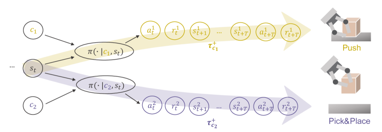
Figure 2: A policy $\pi$ conditioned on a fixed context embedding $c$ is defined as a skill $\pi(\cdot|c)$. Executing different skills (e.g., Push skill $\pi(\cdot|c_{1})$ and Pick&Place skill $\pi(\cdot|c_{2})$) shows different modes of behaviours in trajectories (e.g., $\tau^{+}_{c_{1}}$ where the cube moves on the table; $\tau^{+}_{c_{2}}$ where the cube leaves the table).

2 Related works

Meta-RL. Meta-RL methods train an agent conditioned on context embeddings to improve generalisation to unseen tasks. As the key component of Meta-RL, the quality of the context embedding can significantly affect the agent’s performance. Existing algorithms can be categorised into three types based on different context embeddings. In the first category, the context embedding is learned by minimising the downstream RL loss [Rakelly et al., 2019, Yu et al., 2020]. PEARL [Rakelly et al., 2019] learns probabilistic context embeddings by recovering the value function. Multi-task SAC + TE (TESAC) [Yu et al., 2020] uses the Task Embedding (TE) [Hausman et al., 2018] as input to policies, parameterising the learned policies via a shared embedding space and maximising average returns. However, the update signals from the RL loss are stochastic and weak, and may not capture the similarity relations among tasks [Fu et al., 2021]. The second category involves learning context embeddings through dynamics prediction [Lee et al., 2020, Zhou et al., 2019], which can make the context embeddings noisy, as they may model irrelevant dependencies and overlook task-specific information [Fu et al., 2021]. The third category employs contrastive learning [Fu et al., 2021, Wang et al., 2021, Li et al., 2021, Sang et al., 2022], achieving significant improvements in context learning. However, these methods overlook the similarity of skills between different tasks, thus failing to achieve effective zero-shot generalisation by executing different skills. Our improvements build upon this third category by distinguishing context embeddings according to different optimal skills.

Contrastive learning. Contrastive learning has been applied to RL due to its significant momentum in representation learning in recent years, attributed to its superior effectiveness [Tishby and Zaslavsky, 2015, Hjelm et al., 2019, Dunion and Albrecht, 2024], ease of implementation [Oord et al., 2019], and strong theoretical connection to mutual information (MI) estimation [Poole et al., 2019]. MI is often estimated through noise-contrastive estimation (NCE) [Gutmann and Hyvärinen, 2010], InfoNCE [Oord et al., 2019], and variational objectives [Hjelm et al., 2019]. InfoNCE has garnered recent interest due to its lower variance [Song and Ermon, 2020] and superior performance in downstream tasks. However, InfoNCE may underestimate true MI because it is constrained by the number of samples $K$. To address this issue, CCM [Fu et al., 2021] leverages InfoNCE to learn the context embedding with a large number of samples. DOMINO [Mu et al., 2022] reduces the total MI by introducing an independence assumption; however, this results in biased information. Correspondingly, we focus on proposing an unbiased alternative MI objective and a more data-efficient $K$-sample estimator tailored for downstream RL tasks, which, to our knowledge, have not been addressed in previous research.

3 Preliminaries

Reinforcement learning. In Meta-RL, we assume an environment is a distribution $\xi(e)$ of tasks $e$ (e.g. uniform in our experiments). Each task $e\sim\xi(e)$ has a similar structure that corresponds to a Markov Decision Process (MDP) [Puterman, 2014], defined by $\mathcal{M}_{e}=(\mathcal{S},\mathcal{A},R,P_{e},\gamma)$, with a state space $\mathcal{S}$, an action space $\mathcal{A}$, a reward function $R(s_{t},a_{t})$ where $s_{t}\in\mathcal{S}$ and $a_{t}\in\mathcal{A}$, state transition dynamics $P_{e}(s_{t+1}|s_{t},a_{t})$, and a discount factor $\gamma\in[0,1)$. In order to address the problem of zero-shot generalisation, we consider the transition dynamics $P_{e}(s_{t+1}|s_{t},a_{t})$ vary across tasks $e\sim\xi(e)$ according to multiple environmental features $e=\{e^{0},e^{1},...,e^{N}\}$ that are not included in states $s$ and can be continuous random variables, such as mass and friction, or discrete random variables, such as the cube’s material. For instance, in a cube-moving environment (Figure 1), an agent has different tasks that are defined by different environmental features (e.g., mass and friction). The Meta-RL agent’s goal is to learn a generalisable policy $\pi$ that is robust to such dynamic changes. Specifically, given a set of training tasks $e$ sampled from $\xi_{\text{train}}(e)$, we aim to learn a policy that can maximise the discounted returns, $\arg\max_{\pi}\mathbb{E}_{e\sim\xi_{\text{train}}(e)}[\sum_{t=0}^{\infty}\gamma^{t}R(s_{t},a_{t})|a_{t}\sim\pi(a_{t}|s_{t}),s_{t+1}\sim P_{e}(s_{t+1}|s_{t},a_{t})]$, and can produce accurate control for unseen test tasks $e$ sampled from $\xi_{\text{test}}(e)$.

Contrastive learning. A Meta-RL agent first consumes a collected trajectory $\tau_{t:t+T}=\{s_{t},a_{t},r_{t},s_{t+1},...,s_{t+T},a_{t+T},r_{t+T}\}$ and outputs a context embedding $c$ through a context encoder $\psi(c|\tau_{t:t+T})$, then executes policy $\pi$ conditioned on the current state $s_{t}$ and context embedding $c$ to work across multiple tasks. As a key component, a context encoder $\psi$ captures the unknown context $c$ of the task. We focus on a context encoder that optimises the InfoNCE bound $I_{\text{InfoNCE}}(x;y)$, which is a $K$-sample estimator of the MI $I(x;y)$ [Oord et al., 2019]. Given a query $x$ and a set $Y=\{y_{1},...,y_{K}\}$ of $K$ random samples containing one positive sample $y_{1}$ and $K-1$ negative samples from the distribution $p(y)$, $I_{\text{InfoNCE}}(x;y)$ is obtained by comparing pairs sampled from the joint distribution $x,y_{1}\sim p(x,y)$ to pairs $x,y_{k}$ built using a set of negative examples $y_{2:K}$:

$$I_{\text{InfoNCE}}(x;y|\psi,K)=\mathbb{E}\left[\log\frac{f_{\psi}(x,y_{1})}{\frac{1}{K}\sum_{k=1}^{K}f_{\psi}(x,y_{k})}\right].$$ (1)

InfoNCE constructs a formal lower bound to the MI, i.e., $I_{\text{InfoNCE}}(x;y|\psi,K)\leq I(x;y)$ [Guo et al., 2022, Chen et al., 2021]. Given two inputs $x$ and $y$, their embedding similarity is $f_{\psi}(x,y)=e^{\psi(x)^{\top}\cdot\psi(y_{1})/\beta}$, where $\psi$ is the context encoder that projects $x$ and $y$ into the context embedding space, the dot product is used to calculate the similarity score between $\psi(x),\psi(y)$ pairs [Wu et al., 2018, He et al., 2020], and $\beta$ is a temperature hyperparameter that controls the sensitivity of the product. Some previous Meta-RL methods [Lee et al., 2020, Mu et al., 2022] learn a context embedding $c$ by maximising $I_{\text{InfoNCE}}(c;\tau_{c}|\psi,K)$ between the context $c$ embedded from a trajectory in the current task, and the historical trajectories $\tau_{c}$ under the same environmental features setting.

4 Skill-aware mutual information optimisation for Meta-RL

4.1 The $log$-$K$ curse of $K$-sample MI estimators

In this section, we provide a theoretical analysis of the challenge inherent in learning a $K$-sample estimator for MI, commonly referred to as the $log$-$K$ curse. Based on this theoretical analysis, we give insights to overcome this challenge.

If we have sufficient training epochs for the context encoder $\psi$ in Equation 1 and a sample size $K$, $I_{\text{InfoNCE}}(x;y|\psi,K)\approx\log K$ [Mnih and Teh, 2012, Guo et al., 2022]. Hence, the MI we can optimise is bottlenecked by the number of available samples, formally expressed as:

Lemma 1

Learning a context encoder $\psi$ with a $K$-sample estimator, we always have ${I}_{\text{InfoNCE}}(x;y|\psi,K)$ $\leq$ $\log K$$\leq$$I(x;y)$. (see proof in Appendix A)

To ensure that the $K$-sample estimator is a tight bound of the ground-truth MI, inspired by Lemma 1, we derive three key insights when learning a context encoder: (1) focus on a ground-truth MI that is smaller than $I(x;y)$ and achievable with a smaller sample size; (2) develop a $K$-sample estimator tighter than $I_{\text{InfoNCE}}$; (3) increasing sample quantity $K$, however, this is usually impractical.

A meta-RL agent learns a context encoder by maximising MI between trajectories $\tau_{c}$ and context embeddings $c$. Driven by insight (1), we introduce Skill-aware Mutual Information (SaMI) in Section 4.2, designed to enhance the zero-shot generalisation of downstream RL tasks. Corresponding to insight (2), we propose Skill-aware Noise Contrastive Estimation (SaNCE) to maximise SaMI with limited samples in Section 4.3. Finally, Section 4.4 demonstrates how to equip any Meta-RL agent with SaNCE in practice.

Figure 3: A $K$-sample estimator $I_{\text{InfoNCE}(c;\pi_{c};\tau_{c})}$, with limited sample size $K$, is a loose lower bound of $I(c;\tau_{c})$ and leads to lower performance embeddings. $I_{\text{SaMI}}(c;\pi_{c};\tau_{c})$ is a lower ground-truth MI, and $I_{\text{SaNCE}}(c;\pi_{c};\tau_{c})$ is a tighter lower bound of $I_{\text{SaMI}}(c;\pi_{c};\tau_{c})$.

4.2 Skill-aware mutual information: a smaller ground-truth MI

An useful tool in learning a versatile agent is to understand when to explore novel skills or switch between existing skills in multi-task settings. To start with, we define skills:

Definition 1 (Skills)

A policy $\pi$ conditioned on a fixed context embedding $c$ is defined as a skill $\pi(\cdot|c)$, abbreviated as $\pi_{c}$. If a skill $\pi_{c}$ is conditioned on a state $s_{t}$, we can sample actions $a_{t}\sim\pi(\cdot|c,s_{t})$. If we sample actions from $\pi_{c}$ at consecutive timesteps, we gain a trajectory $\tau_{c}=\{s_{t},a_{t},r_{t},s_{t+1},...,s_{t+T},a_{t+T},r_{t+T}\}$.

After executing skills, an agent should distinguish tasks through environmental feedback to be aware of underlying environmental features $e=\{e^{0},e^{1},...,e^{N}\}$. In this regard, the context encoder $\psi$ should learn by maximising the MI between context embedding $c$, skills $\pi_{c}$, and environmental feedback (i.e., trajectories $\tau_{c}$). We achieve this learning process by maximising the MI $I_{\text{SaMI}}(c;\pi_{c};\tau_{c})$, in which we introduce a variable, skill $\pi_{c}$, into $I(c;\tau_{c})$. Formally, we propose a novel MI optimisation objective for a context encoder, Skill-aware Mutual Information (SaMI), which is defined as:

$$I_{\text{SaMI}}(c;\pi_{c};\tau_{c})=\mathbb{E}_{p(c,\pi_{c},\tau_{c})}\left\{\log\ \frac{p(\tau_{c}|c,\pi_{c})}{p(\tau_{c})}\right\}.$$ (2)

Although we cannot evaluate $p(c,\pi_{c},\tau_{c})$ directly, we approximate it by Monte-Carlo sampling, using $K$ samples from $p(c,\pi_{c},\tau_{c})$. After introducing the variable $\pi_{c}$, $I_{\text{SaMI}}(c;\pi_{c};\tau_{c})$ contains less information, i.e., $I_{\text{SaMI}}(c;\pi_{c};\tau_{c})\leq I(c;\tau_{c})$ (see proof in Appendix B). So the context encoder $\psi$ has a lower ground-truth MI $I_{\text{SaMI}}(c;\pi_{c};\tau_{c})$ to approach. $I_{\text{SaMI}}$ also enables the RL agent to embody diverse skills and switch skills based on the context embedding $c$. In other words, the skill $\pi_{c}$ conditioned on different context embeddings $c$ will exhibit various modes of behaviour, such as the Push skill $\pi_{c_{1}}$ (pushing a cube on the table to the target position) or the Pick&Place skill $\pi_{c_{2}}$.

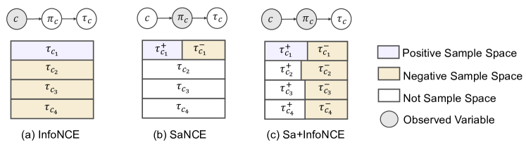
Figure 4: A comparison of sample spaces for task $e_{1}$. Positive samples $\tau_{c_{1}}$ or $\tau_{c_{1}}^{+}$ are always from current task $e_{1}$. For SaNCE, in a task $e_{k}$ with embedding $c_{k}$, the positive skill $\pi_{c_{k}}^{+}$ conditions on $c_{k}$ and generates positive trajectories $\tau_{c_{k}}^{+}$, and the negative skill $\pi_{c_{k}}^{-}$ generates negative trajectories $\tau_{c_{k}}^{-}$. The top graphs show the relationship between $c$, $\pi_{c}$ and $\tau_{c}$.

4.3 Skill-aware noise contrastive estimation: a tighter $K$-sample estimator

Despite InfoNCE’s success as a $K$-sample estimator for approximating MI [Laskin et al., 2020, Eysenbach et al., 2022], its learning efficiency plunges due to limited numerical precision, which is called the $\log$-$K$ curse, i.e., $I_{\text{InfoNCE}}\leq\log K\leq I_{\text{SaMI}}\leq I(c;\tau_{c})$ [Chen et al., 2021] (see proof in Appendix B). When $K\to+\infty$, we can expect $I_{\text{InfoNCE}}\approx\log K\approx I_{\text{SaMI}}$ [Guo et al., 2022]. However, increasing $K$ is too expensive, especially in complex environments with enormous negative sample space. In response, we propose a novel $K$-sample estimator with a reduced required sample space size $K^{*}$ ($K^{*}\ll+\infty$). First, we define $K^{*}$:

Definition 2 ($\mathbf{K^{*}}$)

$K^{*}=|c|\cdot|\pi_{c}|\cdot M$ is defined as the number of trajectories in the replay buffer (i.e., the sample space), in which $|c|$ represents the number of different context embeddings $c$, $|\pi_{c}|$ represents the number of different skills $\pi_{c}$, and $M$ is a natural number.

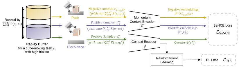
Figure 5: A practical framework for SaNCE. The context encoder embeds the trajectories into context embeddings, in which the queries are generated by context encoder $\psi$ and the negative/positive embeddings are produced by the momentum context encoder $\psi^{*}$. The encoder is updated with gradients from both the SaNCE loss $\mathcal{L}_{\text{SaNCE}}$ and the RL loss $\mathcal{L}_{RL}$. The replay buffer is task-specific.

Note that $K^{*}$ is the maximum batch size that can be sampled in contrastive learning. Therefore, to ensure that $I_{\text{InfoNCE}}$ is a tight bound of $I_{\text{SaMI}}$, we require that $I_{\text{InfoNCE}}\approx\log K\approx I_{\text{SaMI}}$ when $K\to K^{*}$. Under the definition of $K^{*}$, the replay buffer can be divided according to the different context embeddings $c$ and skills $\pi_{c}$ (i.e., observing context embeddings $c$ and skills $\pi_{c}$). In real-world robotic control tasks, the sample space size significantly increases due to multiple environmental features $e=\{e^{0},e^{1},...,e^{N}\}$. Taking the sample space of InfoNCE as an example (Figure 4(a)), in the current task $e_{1}$ with context embedding $c_{1}$, positive samples are trajectories $\tau_{c_{1}}$ generated after executing the skill $\pi_{c_{1}}$ in task $e_{1}$, and negative samples are trajectories $\{\tau_{c_{2}},...\}$ from other tasks $\{e_{2},...\}$. The permutations and combinations of $N$ environmental features lead to an exponential growth in task number $|c|$, which in turn results in an increase of sample space $K^{*}_{\text{InfoNCE}}=|c|\cdot|\pi|\cdot M$.

We introduce a tight $K$-sample estimator, Skill-aware Noise Contrastive Estimation (SaNCE), which is used to approximate $I_{\text{SaMI}}(c;\pi_{c};\tau_{c})$ with a reduced $K^{*}_{\text{SaNCE}}$. For SaNCE, both positive samples $\tau_{c_{1}}^{+}$ and negative samples $\tau_{c_{1}}^{-}$ are sampled from the current tasks $e_{1}$, but are generated by executing positive skills $\pi_{c_{1}}^{+}$ and negative skills $\pi_{c_{1}}^{-}$, respectively. Here, a positive skill is intuitively defined by whether it is optimal for the current task $e$, with a more formal definition provided in Section 4.4. For instance, in a cube-moving task under a large friction setting, the agent executes a skill $\pi_{c}^{+}$ after several iterations of learning, and obtains corresponding trajectories $\tau_{c}^{+}$ where the cubes leave the table surface. This indicates that the skill $\pi_{c}^{+}$ is Pick&Place and other skills $\pi_{c}^{-}$ may include Push or Flip (flipping the cube to the goal position), with corresponding trajectories $\tau_{c}^{-}$ where the cube remains stationary or rolls on the table. Formally, we can optimise the $K$-sample lower bound $I_{\text{SaNCE}}$ to approximate $I_{\text{SaMI}}$:

$$\quad I_{\text{SaNCE}}(c;\pi_{c};\tau_{c}|\psi,K)$$

$$=\mathbb{E}_{p(c_{1},\pi_{c_{1}},\tau_{c_{1}}^{+})p(\tau_{c_{1},2:K}^{-})}\left[\log\left(\frac{K\cdot f_{\psi}(c_{1},\pi_{c_{1}},\tau_{c_{1}}^{+})}{f_{\psi}(c_{1},\pi_{c_{1}},\tau_{c_{1}}^{+})+\sum_{k=2}^{K}f_{\psi}(c_{1},\pi_{c_{1}},\tau_{c_{1},k}^{-})}\right)\right]$$

$$\leq I_{\text{SaMI}}(c;\pi_{c};\tau_{c})$$ (3)

where $f_{\psi}(c_{1},\pi_{c_{1}},\tau_{c_{1}})=e^{\psi(\tau_{c_{1}})^{\top}\cdot\psi^{*}(\tau_{c_{1}})/\beta}$. The query $c_{1}=\psi(\tau_{c_{1}})$ is generated by the context encoder $\psi$. For training stability, we use a momentum encoder $\psi^{*}$ to produce the positive and negative embeddings. SaNCE significantly reduces the required sample space size $K^{*}_{\text{SaNCE}}$ by sampling trajectories $\tau_{c}$ based on different skills $\pi_{c}$ (Figure 4(b)) in task $e_{1}$, so that $K^{*}_{\text{SaNCE}}=|c|\cdot|\pi_{c}|\cdot M=|\pi_{c_{1}}|\cdot M\leq K^{*}_{\text{InfoNCE}}$ ($|c|=|c_{1}|=1$). Therefore, $I_{\text{SaNCE}}$ satisfies Lemma 2:

Lemma 2

With a skill-aware context encoder $\psi$, we have $I_{\text{InfoNCE}}(c;\pi_{c};\tau_{c}|\psi,K)\leq I_{\text{SaNCE}}(c;\pi_{c};\tau_{c}|\psi,K)\leq\log K\leq I_{\text{SaMI}}(c;\pi_{c};\tau_{c})\leq I(c;\tau_{c})$. (see proof in Appendix B)

SaNCE is a plug-and-play module for any other NCE. For example, the negative sample space can be more diverse by combining SaNCE and InfoNCE with $K^{*}_{\text{Sa+InfoNCE}}=\left(\sum_{i=1}^{|c|}|\pi_{c_{i}}^{-}|+|\pi_{c_{1}}^{+}|\right)\cdot M$ (Figure 4(c)). A detailed analysis of the sample size of $I_{\text{Sa+InfoNCE}}$ can be found in Appendix C.

4.4 Optimal/Sub-optimal skill-aware sampling strategy

In this section, we further define the positive and negative skills and propose a practical trajectory sampling method. SaNCE requires sample trajectories by ovserving skills $\pi_{c}$. However, we cannot access the prior distribution $p(\pi_{c})$, making it impossible to enumerate all distinct skills $\pi_{c}$. Therefore, in the optimal/sub-optimal skill-aware sampling method, positive skills $\pi_{c}^{+}$ are defined as the optimal skills achieving the highest return $\sum_{i=t}^{t+T}R(s_{i},a_{i})$ in task $e$, while negative skills $\pi_{c}^{-}$ encompass all the other sub-optimal skills with lower returns in task $e$. Thus, we can simply sample the trajectory with the ranked highest return from the replay buffer as the positive sample $\tau_{c}^{+}$, and the one with the lowest return as the negative sample $\tau_{c}^{-}$. The SaNCE loss is then minimised to bring the context embeddings of the highest return trajectories closer in the embedding space while distancing those of negative trajectories.

Note that, at the end of the training, the top-ranked trajectories in the ranked replay buffer correspond to positive samples $\tau_{c}^{+}$ with high returns, and the lower-ranked ones are negative samples $\tau_{c}^{-}$ with low returns. However, before the agent is able to achieve high returns, all trajectories are with low returns. Therefore, our SaNCE loss is a soft version of the $K$-sample SaNCE estimator:

$$\mathcal{L}_{\text{SaNCE}}=-\max\left(||\psi(\tau_{c}^{+}),\psi(\tau_{c}^{-})||_{L2},1\right)\cdot I_{\text{SaNCE}}$$ (4)

where $||\cdot||_{L2}$ represents the Euclidean distance [Tabak, 2014]. Figure 5 provides a practical framework of SaNCE, with a cube-moving example task $e_{1}$ under high friction. In task $e_{1}$, the positive skill $\pi_{c_{1}}^{+}$ is the Pick&Place skill, which is used to generate queries $\psi(\tau_{c_{1}}^{+})$ and positive embeddings $\psi^{*}(\tau_{c_{1}}^{+})$; after executing Push skill we get negative samples $\tau_{c_{1}}^{-}$ and negative embeddings $\psi^{*}(\tau_{c_{1}}^{-})$.

5 Experiments

We use a three-step process to demonstrate the benefits of SaMI in each environment and answer three questions: (1) Does optimising SaMI lead to increased returns during training and zero-shot generalisation (see Table 5.1 and 2)?; (2) Does SaMI help the RL agents to be versatile and embody multiple skills (see Figure 6)?; (3) Can SaNCE overcome the $\log$-$K$ curse in sample-limited scenarios (see Table 5.1 and 2, and Section 5.4)?

5.1 Experimental setup

Modified benchmarks with multiple environmental features. We demonstrate the efficacy of our method using two benchmarks, Panda-gym [Gallouédec et al., 2021] and MuJoCo [Todorov et al., 2012] (details in Sections 5.2 and 5.3). The benchmarks are modified to be influenced by multiple environmental features simultaneously. Environmental features are sampled at the start of each episode during both training and testing phases. During training, we uniform-randomly select a combination of environmental features from a training set. At test time, we evaluate each algorithm in unseen tasks with different environmental features outside the training range. Generalisation performance is measured in two different regimes: moderate and extreme. The moderate regime draws environmental features from a closer range to the training range compared to the extreme. For all our experiments, we report the mean and standard deviation of the models trained over five seeds in both training and test tasks. Further experimental details are available in Appendix D.

Baselines. In our experiments, we primarily compare InfoNCE with SaNCE to demonstrate the performance improvements brought by SaNCE. Therefore, we compare our method with three prevailing and competitive baselines. First, we consider CCM [Fu et al., 2021], which is equipped with InfoNCE. Additionally, we consider TESAC [Yu et al., 2020], which employs a value function loss, allowing us to evaluate the impact on the context encoder without contrastive loss. Given that CCM and TESAC are using RNN encoder, we also consider PEARL [Rakelly et al., 2019], which utilises an MLP context encoder and a similar loss as TESAC.

Our methods. We employ Soft Actor-Critic (SAC) [Haarnoja et al., 2018] as the base RL algorithm. SaNCE can be integrated with any Meta-RL algorithm. Hence, we equip two RL algorithms with SaNCE: (1) SaTESAC is TESAC with SaNCE, which solely uses SaNCE for contrastive learning, with a significantly smaller sample space than that of other algorithms, as shown in Figure 4(b); (2) SaCCM is CCM with SaNCE, where the contrastive learning combines InfoNCE and SaNCE, as shown in Figure 4(c). The purpose is to compare both the impact of different negative sample spaces on the contrastive learning and downstream RL tasks, and the adaptability of SaNCE across different algorithms. In Appendix G, we provide a comparison in MuJoCo with numerical results from DOMINO [Mu et al., 2022] and CaDM [Lee et al., 2020] because of the exact same environmental setting. The sample spaces of PEARL, TESAC, and CCM are all $|c|$ times larger than that of SaTESAC.

5.2 Panda-gym

Task description. Our modified Panda-gym benchmark contains a robot arm control task using the Franka Emika Panda [Gallouédec et al., 2021], where the robot needs to move a cube to a target position. Unlike previous works, the robot can flexibly execute different skills (Push and Pick&Place) to solve tasks. In our experiments, we simultaneously modify multiple environmental features (cube mass and table friction) that characterise the transition dynamics. In some environmental settings,

Table 1: Comparison of success rate with baselines in Panda-gym (over 5 seeds).The blue background indicates that our method surpasses PEARL, TESAC and CCM. Bold text signifies the highest average return.

	Training	Test (moderate)	Test (extreme)
PEARL	0.42$\pm$0.19	0.10$\pm$0.06	0.11$\pm$0.05
TESAC	0.64$\pm$0.16	0.33$\pm$0.23	0.27$\pm$0.17
CCM	0.82$\pm$0.04	0.50$\pm$0.23	0.29$\pm$0.23
SaTESAC	0.92$\pm$0.05	0.55$\pm$0.25	0.40$\pm$0.35
SaCCM	0.94$\pm$0.02	0.58$\pm$0.27	0.46$\pm$0.36

only a specific skill can accomplish the task. For example, an agent needs to learn the Pick&Place skill to avoid high friction. Thus, the agent must determine when and which skill to execute.

Evaluating zero-shot generalisation. As shown in Table 5.1, SaTESAC and SaCCM achieve superior generalisation performance compared to PEARL, TESAC, and CCM, with a smaller sample space. In training, moderate test, and extreme test tasks, SaTESAC achieved up to 43.75%, 66.67%, and 48.15% higher success rates, respectively, compared to TESAC, while SaCCM improved success rates by 14.63%, 16.00%, and 58.62% compared to CCM.

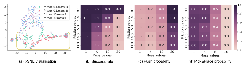
Figure 6: (a) t-SNE visualisation of context embeddings in the Panda-gym environment. The clustered points in the yellow box correspond to the Push skill executed in scenarios with a large mass. Heatmap of (b) success rate, and probability of learned (c) Push skill and (d) Pick&Place skill of SaCCM. Under large mass scenarios, the probability of executing Push skill is higher than Pick&Place skill.

Skill analysis. We visualise the context embedding of SaCCM using t-SNE [Van der Maaten and Hinton, 2008]. We determine the skills by detecting contact points between the end effector and the cube and between the cube and the table (see Appendix D for more details), and then employ Heatmaps [Waskom, 2021] to visualise skills executed by the agent. As shown in Figure 6, we found that when the cube mass is large (30 Kg and 10 Kg), the agent learned the Push skill (corresponding to the clustered points in the yellow bounding box in Figure 6(a). With smaller masses, the agent learned the Pick&Place skill. However, as shown in Figure 15 in Appendix F.1, CCM did not exhibit clear skill grouping. This indicates that SaMI extracts high-quality skill-related information from the trajectories and aids in embodying diverse skills. We provide additional visualisation based on both t-SNE and PCA [Jolliffe, 2002], and heatmap results in Appendix F.

5.3 MuJoCo

Task description. The modified MuJoCo benchmark [Mu et al., 2022, Lee et al., 2020] contains 6 typical robotic control environments based on the MuJoCo physics engine [Todorov et al., 2012]. Hopper, Half-cheetah, Ant, and SlimHumanoid are affected by multiple continuous environmental features (i.e., mass, damping) that characterise the transition dynamics. Both Crippled Ant and Crippled Half-cheetah are more difficult because they are also affected by a discrete environmental feature as one of the actuators in the legs is randomly crippled to change the transition dynamics.

Table 2: Comparison of average return with baselines in modified MuJoCo benchmark (over 5 seeds). The blue background indicates that our method surpasses PEARL, TESAC and CCM. Bold text signifies the highest average return.

	Crippled Ant			Crippled Half-cheetah
	Training	Test (moderate)	Test (extreme)	Training	Test (moderate)	Test (extreme)
PEARL	182$\pm$73	96$\pm$21	88$\pm$31	2538$\pm$783	1028$\pm$445	908$\pm$185
TESAC	485$\pm$83	129$\pm$32	117$\pm$32	4512$\pm$737	1708$\pm$360	1550$\pm$274
CCM	814$\pm$23	146$\pm$13	158$\pm$31	4153$\pm$569	1417$\pm$710	995$\pm$188
SaTESAC	568$\pm$70	176$\pm$9	196$\pm$17	5380$\pm$917	2334$\pm$169	1848$\pm$341
SaCCM	719$\pm$82	215$\pm$6	219$\pm$9	6210$\pm$402	2656$\pm$231	2070$\pm$651
	Ant			Half-cheetah
	Training	Test (moderate)	Test (extreme)	Training	Test (moderate)	Test (extreme)
PEARL	153$\pm$63	73$\pm$25	39$\pm$40	1802$\pm$773	530$\pm$270	346$\pm$102
TESAC	761$\pm$234	360$\pm$23	276$\pm$63	5817$\pm$3064	2843$\pm$1303	1074$\pm$446
CCM	1268$\pm$362	1078$\pm$492	548$\pm$177	6839$\pm$542	3053$\pm$347	1422$\pm$332
SaTESAC	911$\pm$54	590$\pm$111	552$\pm$119	7303$\pm$1353	4077$\pm$424	1723$\pm$88
SaCCM	1015$\pm$60	629$\pm$126	588$\pm$92	7662$\pm$316	4384$\pm$223	1828$\pm$52
	SlimHumanoid			Hopper
	Training	Test (moderate)	Test (extreme)	Training	Test (moderate)	Test (extreme)
PEARL	6947$\pm$3541	3697$\pm$2674	2018$\pm$907	934$\pm$242	874$\pm$366	799$\pm$298
TESAC	9095$\pm$894	7180$\pm$711	3709$\pm$35	1530$\pm$39	1476$\pm$9	1491$\pm$79
CCM	7297$\pm$790	5856$\pm$290	3501$\pm$877	1488$\pm$18	1420$\pm$46	1451$\pm$76
SaTESAC	10501$\pm$2102	8483$\pm$1502	6669$\pm$883	1500$\pm$24	1452$\pm$36	1449$\pm$15
SaCCM	9738$\pm$92	8389$\pm$231	5606$\pm$2027	1472$\pm$53	1456$\pm$13	1446$\pm$94

Results. Table 2 shows the average return of our method and baselines on both training and test tasks. Incorporating SaNCE into TESAC resulted in SaTESAC’s average return increasing by 19.41% in training tasks across all environments, 39.70% in moderate test tasks, and 65.40% in extreme test tasks. Similarly, adding SaNCE to CCM led to SaCCM achieving up to 31.69%, 44.83%, and 40.88% higher average returns in training tasks, moderate test tasks, and extreme test tasks, respectively. Overall, SaTESAC and SaCCM outperform baselines in both training and testing in most of the tasks, in which the Ant, Crippled Ant and Hopper tasks are exceptions. Comparing the visualisation of context embeddings for CCM and SACCM in the Ant, Crippled Ant, and Hopper environments (Appendix F.2), introducing SaNCE does not modify the grouping of context embeddings across different tasks. Notably in Hopper environment, all algorithms maintain consistent average returns when zero-shot generalising to unseen test tasks, with no clear clustering of context embeddings across different tasks (Table 22 in Appendix F.2). This indicates that a single skill may generalise across numerous tasks within the Hopper environment. Hence, we can draw an insight that SaMI is more suitable for environments that require multiple skills to adapt to different environmental features.

5.4 Analysis of the $\log$-$K$ curse in sample-limited scenarios

In this section, we further analyse whether SaNCE can overcome the $\log$-$K$ curse. During the training phases, we sample the environmental features at the beginning of each episode. Therefore, throughout the training process, the context encoder needs to learn the context embedding distribution of multiple tasks. Because InfoNCE requires sampling negative samples across all tasks, and SaNCE samples negative samples from the current task, SaNCE’s negative sample space is $|c|$ times smaller than that of InfoNCE. For example, in the SlimHumanoid environment, where both mass and damping have five values, there can be a maximum of 25 different tasks, making the sampling space of InfoNCE potentially 25 times larger than that of SaNCE. According to Table 5.1 and 2, RL algorithms equipped with SaNCE can achieve better or comparable performance with a much smaller number of negative samples $K$ than InfoNCE. This indicates that SaNCE indeed plays a significant role in addressing the $\log$-$K$ curse, and the SaMI objective helps the contrastive context encoder extract information that is crucial for downstream RL tasks.

Furthermore, the number of negative samples $K$ also relates to two hyperparameters: buffer size, which directly determines the size of the negative sample space; and contrastive batch size, which determines the number of samples used for training contrastive context encoder at each update step. Therefore, we conducted further analysis on these two hyperparameters. As shown in Figure 7, we find that reductions in buffer size and contrastive batch size do not significantly decrease the average return for SaCCM and SaTESAC, which exhibit state-of-the-art performance with small buffers and contrastive batch sizes. Note that the results in Table 2 correspond to a buffer size of 100,000 and a contrastive batch size of 12. Experimental results for all environments (Appendix E.2) further demonstrate that SaNCE is not highly sensitive to changes in $K$, and indeed shows great potential in overcoming the $\log$-$K$ curse.

6 Conclusion and future work

In this paper, we propose a Skill-aware Mutual Information (SaMI) to learn context embeddings for zero-shot generalisation in downstream RL tasks, and a Skill-aware Noise Contrastive Estimation (SaNCE) to optimise SaMI and overcome the $\log$-$K$ curse. RL algorithms equipped with SaMI have achieved state-of-the-art performance in the MuJoCo and Panda-gym benchmarks. Through visual analysis of context embeddings and heatmap analysis of learned skills in Panda-gym, we confirm that SaMI assists the RL agent in embodying diverse skills. These experimental observations indicate that the context encoder, learned by maximising SaMI, helps the RL agent generalise across various tasks by executing different skills. Notably, the optimisation process of SaNCE utilises a far smaller negative sample space than baselines. Coupled with further experimental analysis of buffer size and contrastive batch size on MuJoCo, we demonstrate that SaNCE helps overcome the $\log$-$K$ curse.

Figure 7: Changes of average return in the SlimHumanoid environment. (a) The impact of buffer size on RL control performance (i.e., TESAC, CCM, SaTESAC, SaCCM). (b) The impact of contrastive batch size on the contrastive context encoder (i.e., CCM, SaTESAC, SaCCM).

Our results indicate the importance of aligning the optimisation objectives of representation learning and downstream optimal control to enhance task performance and improve data efficiency.

Given that environmental features are often interdependent, such as a cube’s material correlating with friction and mass, SaMI does not introduce independence assumptions like DOMINO [Mu et al., 2022]. Therefore, future work will focus on verifying and enhancing SaMI’s potential in more complex tasks where environmental features are correlated. This will contribute to our ultimate goal: developing a generalist and versatile agent capable of working across multiple tasks and even real-world tasks in the near future.

Appendix A Proof of Lemma 1

Given a query $x$ and a set $Y=\{y_{1},...,y_{K}\}$ of $K$ random samples containing one positive sample $y_{1}$ and $K-1$ negative samples from the distribution $p(y)$, A $K$-sample InfoNCE estimator is obtained by comparing pairs sampled from the joint distribution $x,y_{1}\sim p(x,y)$ to pairs $x,y_{k}$ built using a set of negative examples $y_{2:K}$. InfoNCE is obtained by comparing positive pairs $(x,y_{1})$ and negative pairs $(x,y_{k})$, where $y_{k}\sim y_{2:K}$, as follows:

$$I_{\text{InfoNCE}}(x;y|\psi,K) =\mathbb{E}_{p(x,y_{1})p(y_{2:K})}\left[\log\left(\frac{f_{\psi}(x,y_{1})}{\frac{1}{K}\sum_{k=1}^{K}f_{\psi}(x,y_{k})}\right)\right]$$ (5)

Step 1. Let us prove the $K$-sample InfoNCE estimator is upper bounded by $\log K$. According to Mu et al. [2022], $\frac{f_{\psi}(x,y_{1})}{\sum_{k=1}^{K}f_{\psi}(x,y_{k})}=\frac{f_{\psi}(x,y_{1})}{f_{\psi}(x,y_{1})+\sum_{k=2}^{K}f_{\psi}(x,y_{k})}\leq 1$. So we have:

$$I_{\text{InfoNCE}}(x;y|\psi,K) =\mathbb{E}_{p(x,y_{1})p(y_{2:K})}\left[\log\left(\frac{f_{\psi}(x,y_{1})}{\frac{1}{K}\sum_{k=1}^{K}f_{\psi}(x,y_{k})}\right)\right]$$

$$=\mathbb{E}_{p(x,y)}\left[\mathbb{E}_{p(y_{2:K})}\log\left(\frac{K\cdot f_{\psi}(x,y_{1})}{\sum_{k=1}^{K}f_{\psi}(x,y_{k})}\right)\right]$$

$$\leq\log K$$ (6)

Hence, we have $I_{\text{InfoNCE}}(x;y|\psi,K)\leq\log K$.

Step 2. We have the $I(x;y)\geq I_{\text{InfoNCE}}(x;y|\psi,K)$ which are rightmost and the leftmost side in Lemma 1 according to:

Proposition 1

[Poole et al., 2019] A $K$-sample estimator is an asymptotically tight lower bound to the MI, i.e.,

$$I(x;y)\geq I_{\text{InfoNCE}}(x;y|\psi,K),\lim_{x\to+\infty}I_{\text{InfoNCE}}(x;y|\psi,K)\to I(x;y)$$

Proof. See Poole et al. [2019] for a neat proof of how the multi-sample estimator (e.g., InfoNCE) lower bounds MI.

Step 3. In this research, the context encoder $\psi$ in $f_{\psi}(x,y)$ is implemented using an RNN to approximate $\frac{p(y|x)}{p(y)}$ [Oord et al., 2019]. For most deep learning platforms, with a powerful learner for $\psi$ and a limited size $K$ such that $I(x;y)\geq\log K$, we can reasonably expect $I_{\text{InfoNCE}}\approx\log K$ after a few training epochs. Therefore, during training, when $K\ll+\infty$, we always have $I(x;y)\geq\log K$.

Proof. See Chen et al. [2021] for more detailed proof.

Step 4. Let us prove that the $K$-sample InfoNCE bound is asymptotically tight. The specific choice of context encoder $\psi$ relates to the tightness of the $K$-sample NCE bound. InfoNCE [Oord et al., 2019] sets $f_{\psi}(x,y)\propto\frac{p(y|x)}{p(y)}$ to model a density ratio which preserves the MI between $x$ and $y$, where $\propto$ stands for ‘proportional to’ (i.e. up to a multiplicative constant). Let us plug in $f_{\psi}(x,y)=f_{\psi}^{*}(x,y)=\frac{p(y|x)}{p(y)}$ into InfoNCE, and we have

$$I_{\text{InfoNCE}}(x;y|\psi,K) =\mathbb{E}\left[\log\left(\frac{f_{\psi}^{*}(x,y_{1})}{\sum_{k=1}^{K}f_{\psi}^{*}(x,y_{k})}\right)\right]+\log K$$

$$=-\mathbb{E}\left[\log\left(1+\frac{p(y)}{p(y|x)}\sum_{k=2}^{K}\frac{p(y_{k}|x)}{p(y_{k})}\right)\right]+\log K$$

$$\approx-\mathbb{E}\left[\log\left(1+\frac{p(y)}{p(y|x)}(K-1)\mathbb{E}_{y_{k}\sim p(y)}\frac{p(y_{k}|x)}{p(y_{k})}\right)\right]+\log K$$

$$=-\mathbb{E}\left[\log\left(1+\frac{p(y_{1})}{p(y_{1}|x)}(K-1)\right)\right]+\log K$$

$$\approx-\mathbb{E}\left[\log\frac{p(y)}{p(y|x)}\right]-\log(K-1)+\log K$$

$$=I(x;y)-\log(K-1)+\log K$$ (7)

Now taking $K\to+\infty$, the last two terms cancel out.

Putting it together. Combining $I(x;y)\geq\log K$ with Proposition 1 and Equation 6, we have Lemma 1:

$${I}_{\text{InfoNCE}}(x;y|\psi,K)\leq\log K\leq I(x;y).$$ (8)

Besides, according to Equation 7, with sample size $K\to+\infty$, $K$-sample InfoNCE bound is sharp and approaches to the true MI $I(x;y)$, i.e., $I_{\text{InfoNCE}}(x;y|\psi,K)\approx\log K\approx I(x;y)$.

Appendix B Proof for Lemma 2

Step 1. According to Lemma 1, we have ${\color[rgb]{0.5625,0.66796875,0.80859375}I_{\text{InfoNCE}}(c;\pi_{c};\tau_{c}|\psi,K)}\leq{\color[rgb]{0.49609375,0.49609375,0.49609375}\log K}\leq{\color[rgb]{0.3828125,0.33984375,0.5859375}I_{\text{SaMI}}(c;\pi_{c};\tau_{c})}$ (shown in Figure 3).

Step 2. Let us prove SaNCE is a $K$-sample SaNCE estimator and upper bounded by ${\color[rgb]{0.49609375,0.49609375,0.49609375}\log K}$. Because $\frac{f_{\psi}(c,\pi_{c},\tau_{c}^{+})}{f_{\psi}(c,\pi_{c},\tau_{c}^{+})+\sum_{k=2}^{K}f_{\psi}(c,\pi_{c},\tau_{c,k}^{-})}\leq 1$ [Mu et al., 2022], so we have:

$$\quad{\color[rgb]{0.78125,0.67578125,0.0390625}I_{\text{SaNCE}}(c;\pi_{c};\tau_{c}|\psi,K)}$$

$$=\mathbb{E}_{p(c_{1},\pi_{c_{1}},\tau_{c_{1}}^{+})p(\tau_{c_{1},2:K}^{-})}\left[\log\left(\frac{K\cdot f_{\psi}(c_{1},\pi_{c_{1}},\tau_{c_{1}}^{+})}{f_{\psi}(c_{1},\pi_{c_{1}},\tau_{c_{1}}^{+})+\sum_{k=2}^{K}f_{\psi}(c_{1},\pi_{c_{1}},\tau_{c_{1},k}^{-})}\right)\right]$$

$$=\mathbb{E}_{p(c_{1},\pi_{c_{1}})}\left[\mathbb{E}_{p(\tau_{c_{1},2:K}^{-})}\log\left(\frac{K\cdot f_{\psi}(c_{1},\pi_{c_{1}},\tau_{c_{1}}^{+})}{f_{\psi}(c_{1},\pi_{c_{1}},\tau_{c_{1}}^{+})+\sum_{k=2}^{K}f_{\psi}(c_{1},\pi_{c_{1}},\tau_{c_{1},k}^{-})}\right)\right]$$

$$\leq{\color[rgb]{0.49609375,0.49609375,0.49609375}\log K}$$ (9)

Hence, we have ${\color[rgb]{0.78125,0.67578125,0.0390625}I_{\text{SaNCE}}(c;\pi_{c};\tau_{c}|\psi,K)}\leq{\color[rgb]{0.49609375,0.49609375,0.49609375}\log K}$ (similar to Equation 6).

Step 3. With the definition of $K^{*}$, we can prove ${\color[rgb]{0.5625,0.66796875,0.80859375}I_{\text{InfoNCE}}(c;\pi_{c};\tau_{c}|\psi,K)}\leq{\color[rgb]{0.78125,0.67578125,0.0390625}I_{\text{SaNCE}}(c;\pi_{c};\tau_{c}|\psi,K)}$ with the same sample size $K$. In task $e_{1}$ with context embedding $c_{1}$, SaNCE obtains positive and negative samples from the current task $e_{1}$. Hence the variable $c=c_{1}$ is constant, we have:

$$\quad{\color[rgb]{0.78125,0.67578125,0.0390625}I_{\text{SaNCE}}(c;\pi_{c};\tau_{c}|\psi,K)}$$

$$=\mathbb{E}_{p(c_{1},\pi_{c_{1}},\tau_{c_{1}}^{+})p(\tau_{c_{1},2:K}^{-})}\left[\log\left(\frac{K\cdot f_{\psi}(c_{1},\pi_{c_{1}},\tau_{c_{1}}^{+})}{f_{\psi}(c_{1},\pi_{c_{1}},\tau_{c_{1}}^{+})+\sum_{k=2}^{K}f_{\psi}(c_{1},\pi_{c_{1}},\tau_{c_{1},k}^{-})}\right)\right]$$

$$\leq\mathbb{E}_{p(c_{1},\pi_{c_{1}},\tau_{c_{1}}^{+})p(\tau_{c_{1},2:K^{*}_{\text{SaNCE}}}^{-})}\left[\log\left(\frac{K^{*}_{\text{SaNCE}}\cdot f_{\psi}(c_{1},\pi_{c_{1}},\tau_{c_{1}}^{+})}{f_{\psi}(c_{1},\pi_{c_{1}},\tau_{c_{1}}^{+})+\sum_{k=2}^{K^{*}_{\text{SaNCE}}}f_{\psi}(c_{1},\pi_{c_{1}},\tau_{c_{1},k}^{-})}\right)\right]$$

$$=\mathbb{E}_{p(\pi_{c_{1}},\tau_{c_{1}}^{+})p(\tau_{c_{1},2:K^{*}_{\text{SaNCE}}}^{-})}\left[\log\left(\frac{K^{*}_{\text{SaNCE}}\cdot f_{\psi}(\pi_{c_{1}},\tau_{c_{1}}^{+})}{f_{\psi}(\pi_{c_{1}},\tau_{c_{1}}^{+})+\sum_{k=2}^{K^{*}_{\text{SaNCE}}}f_{\psi}(\pi_{c_{1}},\tau_{{c_{1}},k}^{-})}\right)\right]\text{($c_{1}$ is constant.)}$$

$$\approx{\color[rgb]{0.49609375,0.49609375,0.49609375}\log K^{*}_{\text{SaNCE}}}$$ (10)

The required sample size $K^{*}_{\text{SaNCE}}=|c_{1}|\cdot|\pi|\cdot M=|\pi|\cdot M$. With $K\to K^{*}_{\text{SaNCE}}$, ${\color[rgb]{0.78125,0.67578125,0.0390625}I_{\text{SaNCE}}(c;\pi_{c};\tau_{c}|\psi,K)}\approx{\color[rgb]{0.3828125,0.33984375,0.5859375}I_{\text{SaMI}}(c;\pi_{c};\tau_{c})}$. Correspondingly, for InfoNCE, in the current task $e_{1}$ with context embedding $c_{1}$, positive samples are trajectories $\tau_{1}$ generated after executing the skill $\pi_{1}$ in task $e_{1}$, and negative samples are trajectories $\{\tau_{c_{2}}^{-},...\}$ from other tasks $\{e_{2},...\}$. Under the definition of $K^{*}$, we have:

$$\quad{\color[rgb]{0.5625,0.66796875,0.80859375}I_{\text{InfoNCE}}(c;\pi_{c};\tau_{c}|\psi,K)}$$

$$=\mathbb{E}_{p(c,\pi_{c},\tau_{c_{1}})p({\tau_{c_{2:|c|},2:K}})}\left[\log\left(\frac{K\cdot f_{\psi}(c,\pi_{c},\tau_{c_{1}})}{f_{\psi}(c,\pi_{c},\tau_{c_{1}})+\sum_{k=2}^{K}f_{\psi}(c,\pi_{c},\tau_{c_{2:|c|},k})}\right)\right]$$

$$\leq\mathbb{E}_{p(c,\pi_{c},\tau_{c_{1}})p(\tau_{c_{2:|c|},2:K^{*}_{\text{InfoNCE}}})}\left[\log\left(\frac{K^{*}_{\text{InfoNCE}}\cdot f_{\psi}(c,\pi_{c},\tau_{c_{1}})}{f_{\psi}(c,\pi_{c},\tau_{c_{1}})+\sum_{k=2}^{K^{*}_{\text{InfoNCE}}}f_{\psi}(c,\pi_{c},\tau_{c_{2:|c|},k})}\right)\right]$$

$$\approx{\color[rgb]{0.49609375,0.49609375,0.49609375}\log K^{*}_{\text{InfoNCE}}},$$ (11)

where $K^{*}_{\text{InfoNCE}}=|c|\cdot|\pi|\cdot M\approx|c|\cdot K^{*}_{\text{SaNCE}}$. In real-world robotic control tasks, the sample space size significantly increases due to multiple environmental features $e=\{e^{0},e^{1},...,e^{N}\}$. $|c|$ is the number of different tasks and increases exponentially due to the permutations and combinations of $N$ environmental features. When current task $e_{1}$ has context embedding $c_{1}$, the $c_{2:|c|}$ refer to the context embedding for the other tasks. With $K\to K^{*}_{\text{InfoNCE}}$, ${\color[rgb]{0.5625,0.66796875,0.80859375}I_{\text{InfoNCE}}(c;\pi_{c};\tau_{c}|\psi,K)}\approx{\color[rgb]{0.3828125,0.33984375,0.5859375}I_{\text{SaMI}}(c;\pi_{c};\tau_{c})}$. Hence, during the training process, ${\color[rgb]{0.5625,0.66796875,0.80859375}I_{\text{InfoNCE}}(c;\pi_{c};\tau_{c}|\psi,K)}\leq{\color[rgb]{0.78125,0.67578125,0.0390625}I_{\text{SaNCE}}(c;\pi_{c};\tau_{c}|\psi,K)}$ with the same sample size $K$.

Step 4. What remains is to show ${\color[rgb]{0.3828125,0.33984375,0.5859375}I_{\text{SaMI}}(c;\pi_{c};\tau_{c})}\leq{\color[rgb]{0.21875,0.328125,0.57421875}I(c;\tau_{c})}$. The MI for three variables is also called interaction information. According to the definition in McGill [1954], the SaMI can be presented as:

Proposition 2

For the case of three variables, the MI could be written as ${\color[rgb]{0.3828125,0.33984375,0.5859375}I_{\text{SaMI}}(c;\pi_{c};\tau_{c})}={\color[rgb]{0.21875,0.328125,0.57421875}I(c;\tau_{c})}-I(c;\tau_{c}|\pi_{c})$.

Using this proposition, one can see that in the case of three variables, interaction information quantifies how much the information shared between two variables differs from what they share if the third variable is known. Several properties of interaction information in the case of three variables have been studied in the literature. Specifically, Yeung [1991] showed that

$$-\min\{I(x;\tau_{c}|\pi_{c}),I(c;\pi_{c}|\tau_{c}),I(\tau_{c};\pi_{c}|c)\}\leq I(c;\tau_{c};\pi_{c})\leq\min\{I(c;\tau_{c}),I(c;\pi_{c}),I(\tau_{c};\pi_{c})\}$$ (12)

Combining Equation 12 and Proposition 2, we have ${\color[rgb]{0.3828125,0.33984375,0.5859375}I_{\text{SaMI}}(c;\pi_{c};\tau_{c})}\leq{\color[rgb]{0.21875,0.328125,0.57421875}I(c;\tau_{c})}$.

Putting it together. Hence, we have Lemma 2: we always have ${\color[rgb]{0.5625,0.66796875,0.80859375}I_{\text{InfoNCE}}(c;\pi_{c};\tau_{c}|\psi,K)}\leq{\color[rgb]{0.78125,0.67578125,0.0390625}I_{\text{SaNCE}}(c;\pi_{c};\tau_{c}|\psi,K)}\leq{\color[rgb]{0.49609375,0.49609375,0.49609375}\log K}\leq{\color[rgb]{0.3828125,0.33984375,0.5859375}I_{\text{SaMI}}(c;\pi_{c};\tau_{c})}\leq{\color[rgb]{0.21875,0.328125,0.57421875}I(c;\tau_{c})}$ (shown in Figure 3), while learning a skill-aware context encoder $\psi$ with SaNCE estimator. $K^{*}_{\text{SaNCE}}<<K^{*}_{\text{InfoNCE}}$ so that $I_{\text{SaNCE}}(c;\pi_{c};\tau_{c}|\psi,K)$ is a much tighter lower bound of the true $I_{\text{SaMI}(c;\pi_{c};\tau_{c})}$ than ${\color[rgb]{0.5625,0.66796875,0.80859375}I_{\text{InfoNCE}}(c;\pi_{c};\tau_{c}|\psi,K)}$.

Appendix C Sample size of $I_{\text{Sa+InfoNCE}}$

We illustrate the sample size of $I_{\text{Sa+InfoNCE}}(c;\pi_{c};\tau_{c}|\psi,K)$ in this section. Sa+InfoNCE plugs SaNCE into InfoNCE, and has positive samples $\tau_{c_{1}}^{+}$ from task $e_{1}$ after executing skill $\pi_{c_{1}}^{+}$, and negative samples are trajectories $\tau_{c_{1:K}}^{-}$ from executing skills $\pi_{c_{1:K}}^{-}$ in task $e_{1:K}$, respectively. Therefore, this is equivalent to observing the variable $c$, then observing the variable $\pi_{c}$, i.e., sampling from the distribution $p(\pi_{c},\tau_{c}|c)p(c)$. We have:

$$I_{\text{Sa+InfoNCE}}(c;\pi_{c};\tau_{c}|\psi,K)$$

$$=\mathbb{E}_{p(c)p(\pi_{c_{1}}^{+},\tau_{c_{1}}^{+}|c)p\left(\left(\pi_{2:|c|}^{-},\tau_{2:|c|}^{-}\right)_{2:K}\right)}\left[\log\left(\frac{K\cdot f_{\psi}(c,\pi_{c_{1}}^{+},\tau_{c_{1}}^{+})}{f_{\psi}(c,\pi_{c_{1}}^{+},\tau_{c_{1}}^{+})+\sum_{k=2}^{K}f_{\psi}(c,\pi_{2:|c|,k}^{-},\tau_{2:|c|,k}^{-})}\right)\right]$$

$$\leq\mathbb{E}_{p(c)p(\pi_{c_{1}}^{+},\tau_{c_{1}}^{+}|c)p\left(\left(\pi_{2:|c|}^{-},\tau_{2:|c|}^{-}\right)_{2:K^{*}_{\text{Sa+InfoNCE}}}\right)}\left[\log\left(\frac{K^{*}_{\text{Sa+InfoNCE}}\cdot f_{\psi}(c,\pi_{c_{1}}^{+},\tau_{c_{1}}^{+})}{f_{\psi}(c,\pi_{c_{1}}^{+},\tau_{c_{1}}^{+})+\sum_{k=2}^{K^{*}_{\text{Sa+InfoNCE}}}f_{\psi}(c,\pi_{2:|c|,k}^{-},\tau_{2:|c|,k}^{-})}\right)\right]$$

$$\approx{\color[rgb]{0.49609375,0.49609375,0.49609375}\log K^{*}_{\text{Sa+InfoNCE}}}$$ (13)

It should be noted that such a combination will increase the size of the negative sample space, i.e., $K^{*}_{\text{Sa+InfoNCE}}=\left(\sum_{i=1}^{|c|}|\pi_{c_{i}}^{-}|+|\pi_{c_{1}}^{+}|\right)\cdot M\geq K^{*}_{\text{SaNCE}}$. Therefore, with the same number $K$ of samples, $I_{\text{Sa+InfoNCE}}$ is less precise and looser than $I_{\text{SaNCE}}$. Hence, a trade-off between sample diversity and the precision of the $K$-sample estimator is required.

Appendix D Environmental setup

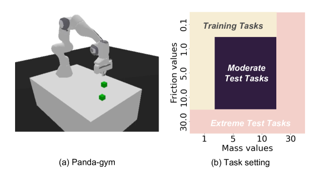
Figure 8: (a) Modified Panda-gym benchmarks, (b) the training tasks, the moderate test tasks and the extreme test tasks. The moderate test task setting just has a combinatorial interpolation. The extreme test task setting has unseen ranges of environmental features and is an extrapolation.

D.1 Modified Panda-gym

We modified the original Pick&Place task in Panda-gym [Gallouédec et al., 2021] by setting the $z$ dimension (i.e., the desired height) of the cube’s goal position equal to $0$ and maintaining the freedom of grippers, so the agent can explore whether it is supposed to push the cube or grasp it. Skills in this benchmark are defined as:

• Pick&Place skill: This skill specifically refers to the agent trying to use the gripper to grasp the cube, pick it up off the table and place it in the goal position. We determine the Pick&Place skill by detecting no contact points between the table and the cube, two contact points between the robot’s end effector and the cube, and the cube’s height being greater than half its width, meaning it is on the table.

• Push skill: This skill refers to the agent giving a push force to the cube and then the cube slides to the goal position. We confirm the Push skill by detecting that the cube’s height is equal to half its width.

• Other skills: Besides the Pick&Place and Push skills, any other different modes of behaviour are classified as other skills. For example, with the Flip skill, the agent applies an initial force to the cube, causing it to roll on the surface or leave the table. In this case, we detect that the cube’s height is greater than half its width, and the number of contact points between the cube and the table is greater than zero.

Some elements in the RL framework are defined as the following:

State space: we use feature vectors which contain cube position (3 dimensions), cube rotation (3 dimensions), cube velocity (3 dimensions), cube angular velocity (3 dimensions), end-effector position (3 dimensions), end-effector velocity (3 dimensions), gripper width (1 dimension), desired goal (3 dimensions) and achieved goal (3 dimensions). Environmental features are not included in the state.

Action space: the action space has 4 dimensions, the first three dimensions are the end-effector’s position changes and the last dimension is the gripper’s width change.

During training, we randomly select a combination of environmental features from a training set sampling combinations from sets: $\text{mass}=1.0$ and $\text{friction}\in\{0.1,1.0,5.0,10.0\}$; $\text{mass}\in\{1.0,5.0,10.0\}$ and $\text{friction}=0.1$. At test time, we evaluate each algorithm in all tasks from the moderate test task setting, in which $\text{mass}\in\{5.0,10.0\}$ and $\text{friction}\in\{1.0,5.0,10.0\}$ (shown in Figure 8(b)), and all tasks from extreme test task setting: $\text{mass}=30.0$ and $\text{friction}\in\{0.1,1.0,5.0,10.0,30.0\}$; $\text{mass}\in\{1.0,5.0,10.0,30.0\}$ and $\text{friction}=30.0$ (shown in Figure 8(b)).

D.2 Modified MuJoCo

We follow exactly the same environmental settings as DOMINO [Mu et al., 2022] and CaDM [Lee et al., 2020]. For Hopper, Half-cheetah, Ant, and SlimHumanoid, we use the environments from the MuJoCo physics engine and use implementation available from Clavera et al. [2019b] and Seo et al. [2020], and scale the mass of every rigid link by scale factor $m$, and scale damping of every joint by scale factor $d$. For Crippled Ant and Crippled Half-cheetah, we use implementation available from Seo et al. [2020] and scale the mass of every rigid link by scale factor $m$, scale damping of every joint by scale factor $d$, and randomly select one leg, and make it crippled to change the dynamic transitions.

Figure 9: Six environments in modified MuJoCo benchmark.

Generalisation performance is measured in two different regimes: moderate and extreme, where the moderate draws environment parameters from a closer range to the training range, compared to the extreme. We have provided our settings for training, extreme and moderate test tasks in Table 3.

Table 3: Environment parameters used for MuJoCo benchmark.

	Training	Test (Moderate)	Test (Extrame)	Episode Length
Half-cheetah	$m\in\{0.75,0.85,1.0,1.15,1.25\}$ $d\in\{0.75,0.85,1.0,1.15,1.25\}$	$m\in\{0.40,0.50,1.50,1.60\}$ $d\in\{0.40,0.50,1.50,1.60\}$	$m\in\{0.20,0.40,1.60,1.80\}$ $d\in\{0.20,0.40,1.60,1.80\}$	1000
Ant	$m\in\{0.75,0.85,1.0,1.15,1.25\}$ $d\in\{0.75,0.85,1.0,1.15,1.25\}$	$m\in\{0.40,0.50,1.50,1.60\}$ $d\in\{0.40,0.50,1.50,1.60\}$	$m\in\{0.20,0.40,1.60,1.80\}$ $d\in\{0.20,0.40,1.60,1.80\}$	1000
Hopper	$m\in\{0.75,1.0,1.25\}$ $d\in\{0.75,1.0,1.25\}$	$m\in\{0.40,0.50,1.50,1.60\}$ $d\in\{0.40,0.50,1.50,1.60\}$	$m\in\{0.20,0.40,1.60,1.80\}$ $d\in\{0.20,0.40,1.60,1.80\}$	500
SlimHumanoid	$m\in\{0.80,0.90,1.0,1.15,1.25\}$ $d\in\{0.80,0.90,1.0,1.15,1.25\}$	$m\in\{0.60,0.70,1.50,1.60\}$ $d\in\{0.60,0.70,1.50,1.60\}$	$m\in\{0.40,0.50,1.70,1.80\}$ $d\in\{0.40,0.50,1.70,1.80\}$	500
Crippled Ant	$m\in\{0.75,0.85,1.0,1.15,1.25\}$ $d\in\{0.75,0.85,1.0,1.15,1.25\}$ Crippled Leg: $\{0,1,2\}$	$m\in\{0.40,0.50,1.50,1.60\}$ $d\in\{0.40,0.50,1.50,1.60\}$ Crippled Leg: $\{3\}$	$m\in\{0.20,0.40,1.60,1.80\}$ $d\in\{0.20,0.40,1.60,1.80\}$ Crippled Leg: $\{3\}$	1000
Crippled Half-cheetah	$m\in\{0.75,0.85,1.0,1.15,1.25\}$ $d\in\{0.75,0.85,1.0,1.15,1.25\}$ Crippled Leg: $\{0,1,2,3\}$	$m\in\{0.40,0.50,1.50,1.60\}$ $d\in\{0.40,0.50,1.50,1.60\}$ Crippled Leg: $\{4,5\}$	$m\in\{0.20,0.40,1.60,1.80\}$ $d\in\{0.20,0.40,1.60,1.80\}$ Crippled Leg: $\{1\}$	1000

D.3 Implementation details

In this section, we provide the implementation details for SaMI. Our codebase is built on top of the publicly released implementation Stable Baselines3 by Raffin et al. [2021] as well as the implementation of InfoNCE by Oord et al. [2019]. A public and open-source implementation of SaMI is available at https://github.com/uoe-agents/SaMI.

Base algorithm. We use SAC [Haarnoja et al., 2018] for downstream evaluation of the learned context embedding. SAC is an off-policy actor-critic method that uses the maximum entropy framework for soft policy iteration. At each iteration, SAC performs soft policy evaluation and improvement steps. We use the same SAC implementation across all baselines and other methods. We trained SAC agents for 1.6 million timesteps on Panda-gym and MuJoCo benchmarks (i.e. Half-cheetah, Ant, Crippled Half-cheetah, Crippled Ant, SlimHumanoid). We evaluated trained agents every $10,000$ timesteps on tasks with fixed random seeds.

Table 4: Hyperparameters used in Panda-gym and MuJoCo benchmarks. Most hyperparameter values are unchanged across tasks except for contrastive batch size and SaNCE loss coefficient.

Hyperparameter	Value
Replay buffer size	100,000
Contrastive batch size	MuJoCo 12, Panda-gym 256
SaNCE loss coefficient $\alpha$	MuJoCo 1.0, Panda-gym 0.01
Context embedding dimension	6
Hidden state dimension	128
Learning rate (actor, critic and encoder)	1e-3
Training frequency (actor, critic and encoder)	128
Gradient steps	16
Momentum context encoder $\psi^{*}$ soft-update rate	0.05
SAC target soft-update rate	critic 0.01, actor 0.05
SAC batch size	256
Discount factor	0.99
Optimizer	Adam

Encoder architecture. For our method, the context encoder $\psi$ is modelled as a Long Short-Term Memory (LSTM) that produces a 128-dimensional hidden state vector, subsequently processed through a single-layer feed-forward network to generate a 6-dimensional context embedding. The actor and critic both use the same context encoder to embed trajectories. For contrastive learning, SaNCE utilises a momentum encoder $\psi^{*}$ to generate positive and negative context embeddings [Laskin et al., 2020, He et al., 2020]. Formally, denoting the parameters of $\psi$ as $\theta_{\psi}$ and those of $\psi^{*}$ as $\theta_{\psi^{*}}$, we update $\theta_{\psi^{*}}$ by:

$$\theta_{\psi^{*}}\leftarrow m\cdot\theta_{\psi}+(1-m)\cdot\theta_{\psi^{*}}.$$ (14)

Here $m\in[0,1)$ is a soft-update rate. Only the parameters $\theta_{\psi}$ are updated by back-propagation. The momentum update in Equation 14 makes $\theta_{\psi^{*}}$ evolve more smoothly by having them slowly track the $\theta_{\psi}$ with $m\ll 1$ (e.g., $m=0.05$ in this research). This means that the target values are constrained to change slowly, greatly improving the stability of learning.

Hyperparameters. A full list of hyperparameters is displayed in Table 4.

Hardware. For each experiment run we use a single NVIDIA Volta V100 GPU with 32GB memory and a single CPU.

Appendix E Additional results

E.1 Balance contrastive and RL updates: loss coefficient $\alpha$

While past work has learned hyperparameters to balance the contrastive loss coefficient $\alpha$ relative to the RL objective [Jaderberg et al., 2016, Bachman et al., 2019], we use both the contrastive and RL objectives together with equal weight $\alpha=1.0$ to be optimal for the MuJoCo benchmark, and $\alpha=0.01$ for the Panda-gym benchmark, we also analyse the effect of loss coefficient $\alpha$ for CCM, SaTESAC and SaCCM in MuJoCo (Figure 11) and Panda-gym (Figure 10) benchmarks.

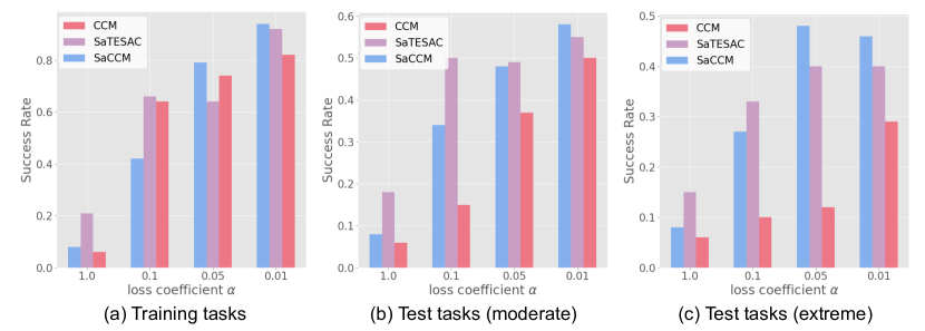
Figure 10: Loss coefficient $\alpha$ analysis of Panda-gym benchmark in training and test (moderate and extreme) tasks.

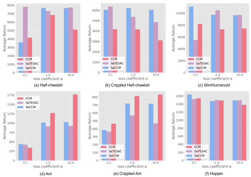
Figure 11: Loss coefficient $\alpha$ analysis of MuJoCo benchmark in training tasks.

E.2 Result of $\log$-$K$ curse analysis

E.2.1 Buffer size

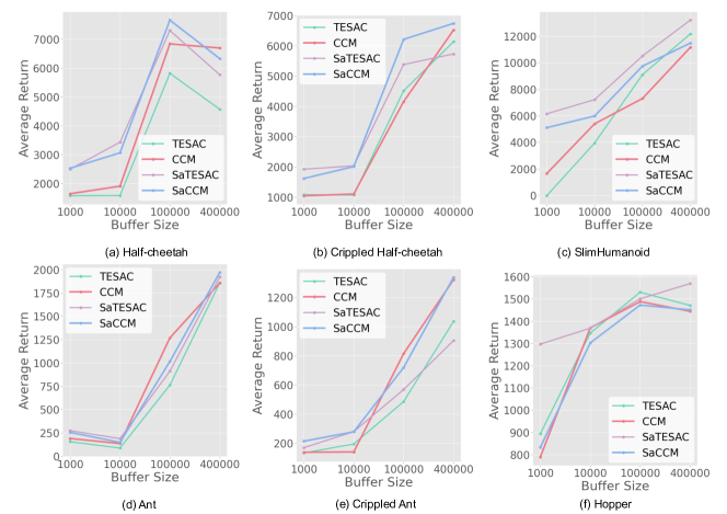
Figure 12: Comparison of different buffer sizes in MuJoCo benchmark in training tasks (over 5 seeds). Buffer size = 400000, 100000, 10000, and 1000.

E.2.2 contrastive batch size

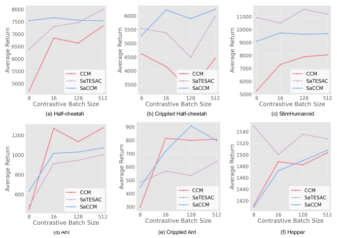
Figure 13: Comparison of different contrastive batch sizes in MuJoCo benchmark in training tasks (over 5 seeds). contrastive batch size = 512, 128, 16, and 8.

Appendix F Further skill analysis

F.1 Panda-gym

F.1.1 Visualisation of context embedding

We visualise the context embedding via t-SNE [Van der Maaten and Hinton, 2008] (Figure 15) and PCA [Jolliffe, 2002] (Figure 14). We found that when the mass of the cube is high (30 Kg and 10 Kg), the agent learned the Push skill (the yellow bounding box in Figure 5.1(a)), whereas with lower masses, the agent learned the Pick&Place skill. However, as shown in Figure 15(b), CCM did not display clear skill grouping. This indicates that SaMI extracts high-quality skill-related information from the trajectories and helps with embodying diverse skills.

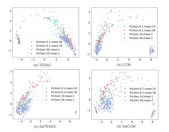
Figure 14: PCA visualization of context embedding extracted from trajectories collected in Panda-gym environments.

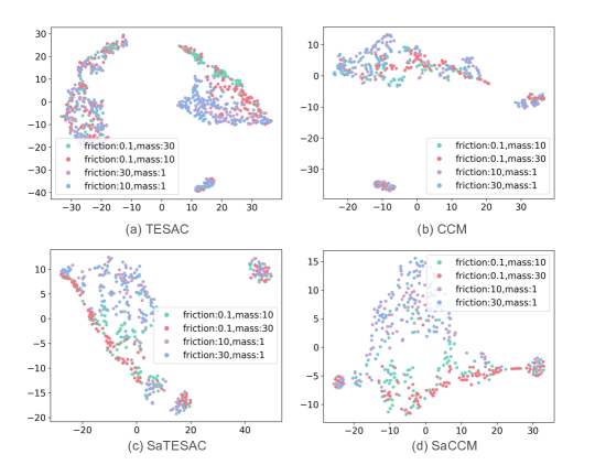
Figure 15: t-SNE visualization of context embedding extracted from trajectories collected in Panda-gym environments.

F.1.2 Heatmap of Panda-gym benchmark

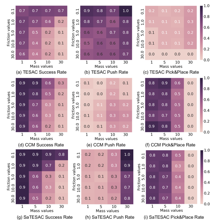
Figure 16: Heatmap of success rate and learned skills of SaCCM. For each grid, the $(i,j)^{th}$ location shows the probability of the skills executed in 100 evaluations with $(\text{mass}=i,\text{friction}=j)$. We determine the skills by detecting contact points between the end effector and the cube and between the cube and the table.

This section provides the heatmap results and further analysis of TESAC, CCM, and SaTESAC on the Panda-gym benchmark. Initially, from the heatmap results of SaTESAC and SaCCM (Figure 6), we observed that with higher cube masses (30 and 10 kg), the agent adopted the Push skill (as indicated by the clustered points in the yellow bounding box in Figure 5.1(a)). At lower masses, the agent adopted the Pick&Place skill.

In contrast to CCM, as seen in Figures 16(e-f), CCM predominantly learned the Pick&Place skill, resulting in a decline in success rates for tasks at $mass=30$, as the agent could not lift the cube off the table using the Pick&Place skill, as depicted in Figure 16(d). The visualisation of the context embedding (Figure 15) did not show clear grouping across different tasks.

Finally, TESAC only mastered the Push skill. The Push skill is relatively simpler to learn than the Pick&Place skill, as it does not require the agent to master manipulating fingers to pick up cubes. Consequently, TESAC’s success rate notably decreased in environments with higher friction.

F.2 MuJoCo

We find that SaMI help the RL agents be versatile and embody multiple skills. For example, Figure 17 displays the t-SNE visualization results of four methods in the Crippled Half-cheetah environment for both test (moderate and extreme) and training tasks. Tasks corresponding to different crippled joints on the same leg are clustered together. Further, we have displayed rendered videos (https://github.com/uoe-agents/SaMI) to better demonstrate the different skills learned.

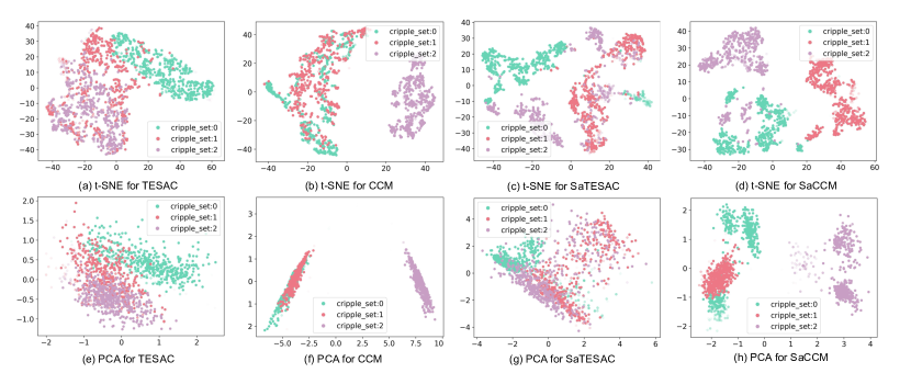
Figure 17: t-SNE and PCA visualisation of context embedding extracted from trajectories collected in Crippled Half-cheetah environment.

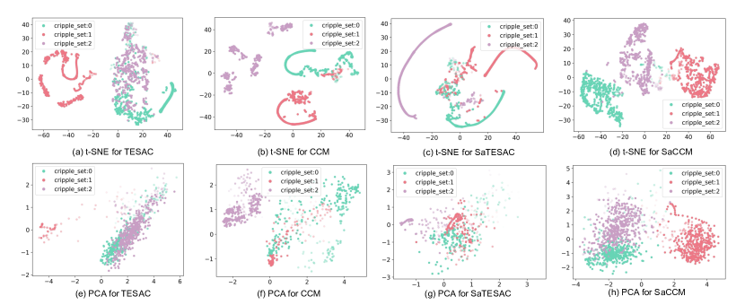
Figure 18: t-SNE and PCA visualization of context embedding extracted from trajectories collected in Crippled Ant environment.

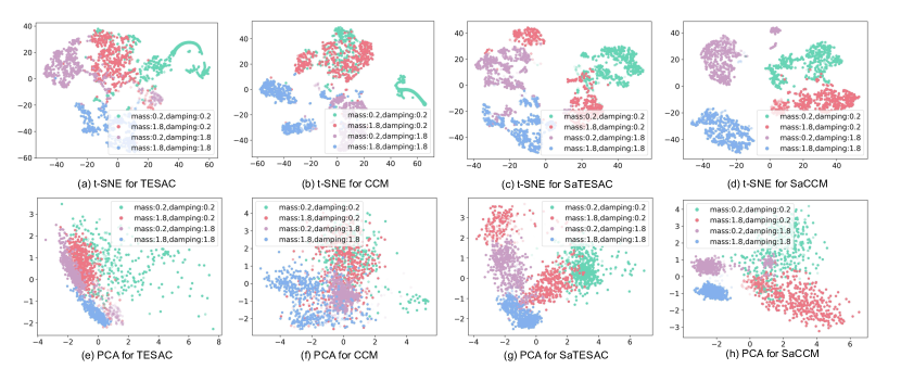
Figure 19: t-SNE and PCA visualization of context embedding extracted from trajectories collected in Half-cheetah environment.

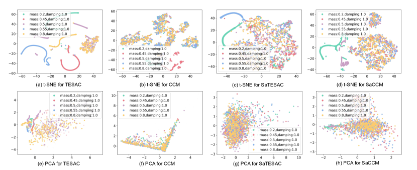
Figure 20: t-SNE and PCA visualization of context embedding extracted from trajectories collected in Ant environment.

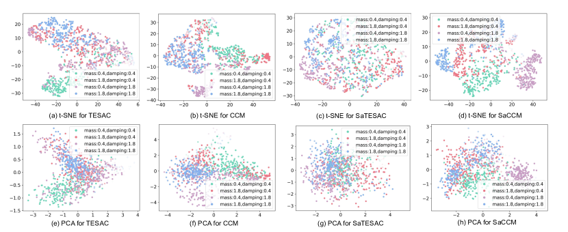
Figure 21: t-SNE and PCA visualization of context embedding extracted from trajectories collected in SlimHumanoid environment.

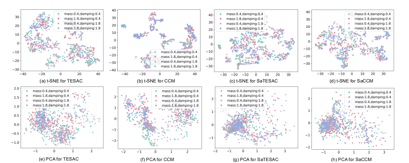
Figure 22: t-SNE and PCA visualization of context embedding extracted from trajectories collected in Hopper environment.

Table 5: Sub-standard comparison of average return with baselines in MuJoCo benchmark (over 5 seeds). The blue background indicates that our method surpasses the baseline, and bold text signifies the highest average return. The numerical results for PPO+DOMINO are copied from Mu et al. [2022]; the numerical results for PPO+CaDM, Vanilla+CaDM, and PE-TS+CaDM are copied from Lee et al. [2020].

	Ant			Half-cheetah
	Training	Test (moderate)	Test (extreme)	Training	Test (moderate)	Test (extreme)
PPO+DOMINO	227$\pm$86	216$\pm$52		2472$\pm$803	1034$\pm$476
PPO+CaDM	268.6$\pm$77.0	228.8$\pm$48.4	199.2$\pm$52.1	2652.0$\pm$1133.6	1224.2$\pm$630.0	1021.1$\pm$676.6
Vanilla+CaDM	1851.0$\pm$113.7	1315.7$\pm$45.5	821.4$\pm$113.5	3536.5$\pm$641.7	1556.1$\pm$260.6	1264.5$\pm$228.7
PE-TS+CaDM	2848.4$\pm$61.9	2121.0$\pm$60.4	1200.7$\pm$21.8	8264.0$\pm$1374.0	7087.2$\pm$1495.6	4661.8$\pm$783.9
SaTESAC	911$\pm$54	590$\pm$111	552$\pm$119	7303$\pm$1353	4077$\pm$424	1723$\pm$88
SaCCM	1015$\pm$60	629$\pm$126	588$\pm$92	7662$\pm$316	4384$\pm$223	1828$\pm$52
	SlimHumanoid			Handcapped Half-Cheetah
	Training	Test (moderate)	Test (extreme)	Training	Test (moderate)	Test (extreme)
PPO+DOMINO	7825$\pm$1256	5258$\pm$1039		2503$\pm$658	1326$\pm$491
PPO+CaDM	10455.0$\pm$1004.9	4975.7$\pm$1305.7	3015.1$\pm$1508.3	2356.6$\pm$624.3	1454.0$\pm$462.6	1025.0$\pm$296.2
Vanilla+CaDM	1758.2$\pm$459.1	1228.9$\pm$374.0	1487.9$\pm$339.0	2435.1$\pm$880.4	1375.3$\pm$290.6	966.9$\pm$89.4
PE-TS+CaDM	1371.9$\pm$400.0	903.7$\pm$343.9	814.5$\pm$274.8	3294.9$\pm$733.9	2618.7$\pm$647.1	1294.2$\pm$214.9
SaTESAC	10501$\pm$2102	8483$\pm$1502	6669$\pm$883	5380$\pm$917	2334$\pm$169	1848$\pm$341
SaCCM	9738$\pm$92	8389$\pm$231	5606$\pm$2027	6210$\pm$402	2656$\pm$231	2070$\pm$651

Appendix G A comparison with DOMINO and CaDM

In this section, we give a brief comparison between our methods and methods from DOMINO [Mu et al., 2022] and CaDM [Lee et al., 2020] in the MuJoCo benchmark because we are using the exact same environmental setting.

DOMINO [Mu et al., 2022] is based on the InfoNCE $K$-sample estimator. Their implementation, PPO+DOMINO, is a model-free RL algorithm with a pre-trained context encoder. This encoder reduces the demand for large contrastive batch sizes during training by decoupling representation learning for each modality, simplifying tasks while leveraging shared information. However, a pre-trained encoder necessitates a large sample volume, with DOMINO training PPO agents for 5 million timesteps on the MuJoCo benchmark. In contrast, SaTESAC and SaCCM, trained for 1.6 million timesteps without pre-trained encoders, achieve considerably higher average returns across four environments (Table 5). Therefore, it is crucial to focus on extracting mutual information in contrastive learning that directly optimises downstream tasks, integrating rather than segregating representation learning from task performance.

CaDM [Lee et al., 2020] proposes a context-aware dynamics model adaptable to changes in dynamics. Specifically, they utilise contrastive learning to learn context embeddings, and then predict the next state conditioned on them. We copy the numerical results of PPO+CaDM, Vanilla+CaDM, and PE-TS+CaDM from CaDM [Lee et al., 2020] as their environmental setting is identical to ours, where PPO+CaDM is a model-free RL algorithm, while Vanilla+CaDM and PE-TS+CaDM are model-based. The model-free RL approach, PPO+CaDM, is trained for 5 million timesteps on the MuJoCo benchmark. As shown in Table 5, SaTESAC and SaCCM significantly outperform PPO+CaDM. The model-based RL algorithms, Vanilla+CaDM and PE-TS+CaDM, require 2 million timesteps for learning in model-based setups, compared to our fewer samples (i.e., million timesteps). In the Ant environment, Vanilla+CaDM and PE-TS+CaDM achieve higher returns than SaTESAC and SaCCM; similarly, in the Half-cheetah environment, PE-TS+CaDM outperforms them. Results in the SlimHumanoid and Crippled Half-cheetah environments show that skill-aware context embeddings are notably effective. An insight here is that our method outperforms the model-free CaCM approach, but not the model-based one. Therefore, we consider that a model-based approach to SaMI could be an interesting extension for future work.

References

- Agarwal et al. [2021] Rishabh Agarwal, Marlos C Machado, Pablo Samuel Castro, and Marc G Bellemare. Contrastive behavioral similarity embeddings for generalization in reinforcement learning. arXiv preprint arXiv:2101.05265, 2021.
- Arora et al. [2019] Sanjeev Arora, Hrishikesh Khandeparkar, Mikhail Khodak, Orestis Plevrakis, and Nikunj Saunshi. A theoretical analysis of contrastive unsupervised representation learning. arXiv preprint arXiv:1902.09229, 2019.
- Bachman et al. [2019] Philip Bachman, R Devon Hjelm, and William Buchwalter. Learning representations by maximizing mutual information across views. Advances in neural information processing systems, 32, 2019.
- Chen et al. [2021] Junya Chen, Zhe Gan, Xuan Li, Qing Guo, Liqun Chen, Shuyang Gao, Tagyoung Chung, Yi Xu, Belinda Zeng, Wenlian Lu, et al. Simpler, faster, stronger: Breaking the log-k curse on contrastive learners with flatnce. arXiv preprint arXiv:2107.01152, 2021.
- Clavera et al. [2019a] Ignasi Clavera, Anusha Nagabandi, Simin Liu, Ronald S. Fearing, Pieter Abbeel, Sergey Levine, and Chelsea Finn. Learning to adapt in dynamic, real-world environments through meta-reinforcement learning. In International Conference on Learning Representations, 2019a.
- Clavera et al. [2019b] Ignasi Clavera, Anusha Nagabandi, Simin Liu, Ronald S. Fearing, Pieter Abbeel, Sergey Levine, and Chelsea Finn. Learning to adapt in dynamic, real-world environments through meta-reinforcement learning. In International Conference on Learning Representations, 2019b.
- des Combes et al. [2018] Remi Tachet des Combes, Philip Bachman, and Harm van Seijen. Learning invariances for policy generalization, 2018. URL https://openreview.net/forum?id=BJHRaK1PG.
- Dunion and Albrecht [2024] Mhairi Dunion and Stefano V Albrecht. Multi-view disentanglement for reinforcement learning with multiple cameras. In Reinforcement Learning Conference, 2024.
- Dunion et al. [2023a] Mhairi Dunion, Trevor McInroe, Kevin Sebastian Luck, Josiah P. Hanna, and Stefano V Albrecht. Conditional mutual information for disentangled representations in reinforcement learning. In Thirty-seventh Conference on Neural Information Processing Systems, 2023a.
- Dunion et al. [2023b] Mhairi Dunion, Trevor McInroe, Kevin Sebastian Luck, Josiah P. Hanna, and Stefano V Albrecht. Temporal disentanglement of representations for improved generalisation in reinforcement learning. In The Eleventh International Conference on Learning Representations, 2023b.
- Eysenbach et al. [2022] Benjamin Eysenbach, Tianjun Zhang, Sergey Levine, and Russ R Salakhutdinov. Contrastive learning as goal-conditioned reinforcement learning. Advances in Neural Information Processing Systems, 35:35603–35620, 2022.
- Franke et al. [2021] Jörg K.H. Franke, Gregor Koehler, André Biedenkapp, and Frank Hutter. Sample-efficient automated deep reinforcement learning. In International Conference on Learning Representations, 2021.
- Fu et al. [2021] Haotian Fu, Hongyao Tang, Jianye Hao, Chen Chen, Xidong Feng, Dong Li, and Wulong Liu. Towards effective context for meta-reinforcement learning: an approach based on contrastive learning. In Proceedings of the AAAI Conference on Artificial Intelligence, pages 7457–7465, 2021.
- Gallouédec et al. [2021] Quentin Gallouédec, Nicolas Cazin, Emmanuel Dellandréa, and Liming Chen. panda-gym: Open-Source Goal-Conditioned Environments for Robotic Learning. 4th Robot Learning Workshop: Self-Supervised and Lifelong Learning at NeurIPS, 2021.
- Garcin et al. [2024] Samuel Garcin, James Doran, Shangmin Guo, Christopher G. Lucas, and Stefano V. Albrecht. DRED: Zero-shot transfer in reinforcement learning via data-regularised environment design. In International Conference on Machine Learning (ICML), 2024.
- Guo et al. [2022] Qing Guo, Junya Chen, Dong Wang, Yuewei Yang, Xinwei Deng, Jing Huang, Larry Carin, Fan Li, and Chenyang Tao. Tight mutual information estimation with contrastive fenchel-legendre optimization. Advances in Neural Information Processing Systems, 35:28319–28334, 2022.
- Gutmann and Hyvärinen [2010] Michael Gutmann and Aapo Hyvärinen. Noise-contrastive estimation: A new estimation principle for unnormalized statistical models. In Proceedings of the thirteenth international conference on artificial intelligence and statistics, pages 297–304. JMLR Workshop and Conference Proceedings, 2010.
- Haarnoja et al. [2018] Tuomas Haarnoja, Aurick Zhou, Pieter Abbeel, and Sergey Levine. Soft actor-critic: Off-policy maximum entropy deep reinforcement learning with a stochastic actor. In International conference on machine learning, pages 1861–1870. PMLR, 2018.
- Hausman et al. [2018] Karol Hausman, Jost Tobias Springenberg, Ziyu Wang, Nicolas Heess, and Martin Riedmiller. Learning an embedding space for transferable robot skills. In International Conference on Learning Representations, 2018.
- He et al. [2020] Kaiming He, Haoqi Fan, Yuxin Wu, Saining Xie, and Ross Girshick. Momentum contrast for unsupervised visual representation learning. In Proceedings of the IEEE/CVF conference on computer vision and pattern recognition, pages 9729–9738, 2020.
- Hjelm et al. [2019] R Devon Hjelm, Alex Fedorov, Samuel Lavoie-Marchildon, Karan Grewal, Phil Bachman, Adam Trischler, and Yoshua Bengio. Learning deep representations by mutual information estimation and maximization. In International Conference on Learning Representations, 2019.
- Jaderberg et al. [2016] Max Jaderberg, Volodymyr Mnih, Wojciech Marian Czarnecki, Tom Schaul, Joel Z Leibo, David Silver, and Koray Kavukcuoglu. Reinforcement learning with unsupervised auxiliary tasks, 2016.
- Jolliffe [2002] Ian T Jolliffe. Principal component analysis for special types of data. Springer, 2002.
- Laskin et al. [2020] Michael Laskin, Aravind Srinivas, and Pieter Abbeel. Curl: Contrastive unsupervised representations for reinforcement learning. In International conference on machine learning, pages 5639–5650. PMLR, 2020.
- Lee et al. [2020] Kimin Lee, Younggyo Seo, Seunghyun Lee, Honglak Lee, and Jinwoo Shin. Context-aware dynamics model for generalization in model-based reinforcement learning. In International Conference on Machine Learning, pages 5757–5766. PMLR, 2020.
- Li et al. [2021] Lanqing Li, Yuanhao Huang, Mingzhe Chen, Siteng Luo, Dijun Luo, and Junzhou Huang. Provably improved context-based offline meta-rl with attention and contrastive learning. arXiv preprint arXiv:2102.10774, 2021.
- McGill [1954] William McGill. Multivariate information transmission. Transactions of the IRE Professional Group on Information Theory, 4(4):93–111, 1954.
- Mnih and Teh [2012] Andriy Mnih and Yee Whye Teh. A fast and simple algorithm for training neural probabilistic language models. arXiv preprint arXiv:1206.6426, 2012.
- Mu et al. [2022] Yao Mu, Yuzheng Zhuang, Fei Ni, Bin Wang, Jianyu Chen, Jianye HAO, and Ping Luo. DOMINO: Decomposed mutual information optimization for generalized context in meta-reinforcement learning. In Alice H. Oh, Alekh Agarwal, Danielle Belgrave, and Kyunghyun Cho, editors, Advances in Neural Information Processing Systems, 2022.
- Nozawa and Sato [2021] Kento Nozawa and Issei Sato. Understanding negative samples in instance discriminative self-supervised representation learning. Advances in Neural Information Processing Systems, 34:5784–5797, 2021.
- Oord et al. [2019] Aaron van den Oord, Yazhe Li, and Oriol Vinyals. Representation learning with contrastive predictive coding. arXiv preprint arXiv:1807.03748, 2019.
- Poole et al. [2019] Ben Poole, Sherjil Ozair, Aaron Van Den Oord, Alex Alemi, and George Tucker. On variational bounds of mutual information. In International Conference on Machine Learning, pages 5171–5180. PMLR, 2019.
- Puterman [2014] Martin L Puterman. Markov decision processes: discrete stochastic dynamic programming. John Wiley & Sons, 2014.
- Raffin et al. [2021] Antonin Raffin, Ashley Hill, Adam Gleave, Anssi Kanervisto, Maximilian Ernestus, and Noah Dormann. Stable-baselines3: Reliable reinforcement learning implementations. Journal of Machine Learning Research, 22(268):1–8, 2021. URL http://jmlr.org/papers/v22/20-1364.html.
- Rakelly et al. [2019] Kate Rakelly, Aurick Zhou, Chelsea Finn, Sergey Levine, and Deirdre Quillen. Efficient off-policy meta-reinforcement learning via probabilistic context variables. In International conference on machine learning, pages 5331–5340. PMLR, 2019.
- Sang et al. [2022] Tong Sang, Hongyao Tang, Yi Ma, Jianye Hao, Yan Zheng, Zhaopeng Meng, Boyan Li, and Zhen Wang. Pandr: Fast adaptation to new environments from offline experiences via decoupling policy and environment representations, 2022.
- Seo et al. [2020] Younggyo Seo, Kimin Lee, Ignasi Clavera Gilaberte, Thanard Kurutach, Jinwoo Shin, and Pieter Abbeel. Trajectory-wise multiple choice learning for dynamics generalization in reinforcement learning. Advances in Neural Information Processing Systems, 33:12968–12979, 2020.
- Song and Ermon [2020] Jiaming Song and Stefano Ermon. Understanding the limitations of variational mutual information estimators. In International Conference on Learning Representations, 2020.
- Tabak [2014] John Tabak. Geometry: the language of space and form. Infobase Publishing, 2014.
- Tishby and Zaslavsky [2015] Naftali Tishby and Noga Zaslavsky. Deep learning and the information bottleneck principle. In 2015 ieee information theory workshop (itw), pages 1–5. IEEE, 2015.
- Todorov et al. [2012] Emanuel Todorov, Tom Erez, and Yuval Tassa. Mujoco: A physics engine for model-based control. In 2012 IEEE/RSJ international conference on intelligent robots and systems, pages 5026–5033. IEEE, 2012.
- Van der Maaten and Hinton [2008] Laurens Van der Maaten and Geoffrey Hinton. Visualizing data using t-sne. Journal of machine learning research, 9(11), 2008.
- Wang et al. [2021] Bernie Wang, Simon Xu, Kurt Keutzer, Yang Gao, and Bichen Wu. Improving context-based meta-reinforcement learning with self-supervised trajectory contrastive learning, 2021.
- Waskom [2021] Michael L. Waskom. seaborn: statistical data visualization. Journal of Open Source Software, 6(60):3021, 2021. doi: 10.21105/joss.03021. URL https://doi.org/10.21105/joss.03021.
- Wu et al. [2018] Zhirong Wu, Yuanjun Xiong, Stella X Yu, and Dahua Lin. Unsupervised feature learning via non-parametric instance discrimination. In Proceedings of the IEEE conference on computer vision and pattern recognition, pages 3733–3742, 2018.
- Yeung [1991] Raymond W Yeung. A new outlook on shannon’s information measures. IEEE transactions on information theory, 37(3):466–474, 1991.
- Yu et al. [2020] Tianhe Yu, Deirdre Quillen, Zhanpeng He, Ryan Julian, Karol Hausman, Chelsea Finn, and Sergey Levine. Meta-world: A benchmark and evaluation for multi-task and meta reinforcement learning. In Conference on robot learning, pages 1094–1100. PMLR, 2020.
- Zhou et al. [2019] Wenxuan Zhou, Lerrel Pinto, and Abhinav Gupta. Environment probing interaction policies. In International Conference on Learning Representations, 2019.