Quasinormal modes and ringdown waveforms of the Frolov black hole

Abstract

In this paper, we investigate the scalar perturbation over the Frolov black hole (BH), which is a regular BH induced by the quantum gravity effect. The quasinormal frequencies (QNFs) of scalar field always consistently reside in the lower half-plane, and its time-domain evolution demonstrates a decaying behavior, with the late-time tail exhibiting a power-law pattern. These observations collectively suggest the stability of the Frolov BH against the scalar perturbation. Additionally, our study reveals that the quantum gravity effect lead to slower decay modes. For the case of the angular quantum number $l=0$, the oscillation exhibits non-monotonic behavior with the quantum gravity parameter $\alpha_{0}$. However, once $l\geq 1$, the angular quantum number surpasses the influence of the quantum gravity effect.

I Introduction

Regular black holes (BHs) were originally introduced as a means to circumvent the central singularity inherent in ordinary BHs. Regular BHs may be categorized into two types based on their asymptotic behavior approaching the center: those with a de-Sitter (dS) core and those with a Minkowskian core. Notable examples of the regular BHs with dS core are the Bardeen BH Bardeen:1968 , Hayward BH Hayward:2005gi , and Frolov BH Frolov:2016pav . The regular BH with Minkowskian core is usually characterized by the exponential potentials, as described in the references Xiang:2013sza ; Culetu:2013fsa ; Culetu:2014lca ; Rodrigues:2015ayd ; Simpson:2019mud ; Ghosh:2014pba ; Ghosh:2018bxg ; Li:2016yfd ; Martinis:2010zk ; Ling:2021olm . To find comprehensive reviews on regular BHs, kindly consult the references Bambi:2023try ; Vagnozzi:2022moj ; Lan:2023cvz . This research aims to analyze the characteristics of the quasinormal modes (QNMs) of the Frolov BH.

Perturbing a BH and observing its response are widely recognized as a powerful method for extracting crucial characteristics of the BH. This perturbation can be implemented either by introducing a probe matter field into its spacetime by hand or by physically perturbing its metric. Perturbing the metric leads to the emission of gravitational waves (GWs). Prior to reaching the equilibrium, the system undergoes a phase of BH merging referred to as the ringdown phase. During this stage, the BH releases GWs with characteristic discrete frequencies, i.e., quasinormal frequencies (QNFs). These frequencies encode information about the decaying scales and damped oscillations of the BH Berti:2009kk . Studying the properties of QNFs offers an opportunity to detect deviations from General Relativity (GR) or even quantum gravity effects through GW observations. However, the majority of regular BHs are typically constructed by incorporating quantum gravity effects at the phenomenological level, making it challenging to establish consistently effective gravitational perturbation equations. Fortunately, even when only a probe matter field is considered over these regular BHs, their QNM spectra are also influenced by the background spacetime. Therefore, these QNM spectra also provide crucial information about the internal structure of the BH and can be used to model the GW form during the ringdown phase at a phenomenological level Berti:2005ys ; Berti:2018vdi ; Fu:2022cul ; Fu:2023drp ; Gong:2023ghh .

In Ref. Lopez:2018aec , the authors investigated the properties of QNMs for a probe massless scalar field over the Frolov BH in the eikonal limit, i.e, the large angular quantum number. The effective potential for the Frolov BH is found to be higher than that of the uncharged Hayward BH. The imaginary parts of the QNFs for the Frolov BH grow with the charge and exhibits a maximum, followed by a more pronounced decrease for small values of the parameter associated with the effective cosmological constant at small distances. As the charge grows, so do the real parts of the QNFs. In this work, we will conduct a systematic investigation of the QNMs of the Frolov BH, with a primary focus on the case of low angular quantum numbers, in contrast to the eikonal limit studied in Lopez:2018aec .

Our paper is organized as follows. In Section II, we offer a concise overview of the Frolov BH along with its fundamental properties, and we also introduce the dynamics of the scalar field over the Frolov BH. In Section IV, we provide a concise introduction to the pseudospectral method. The characteristics of the QNMs and the ringdown waveforms of the scalar field over the Frolov BH are discussed in Section IV and Section V, respectively. Conclusions and further discussions are presented in Section VI.

II Probe scalar field over the Frolov black hole

The Frolov BH is an extension of the Hayward BH to the charged case, originally proposed in Frolov:2016pav . The geometry of the Frolov regular BH is described by Frolov:2016pav :

$$\textrm{d}s^{2}=-f(r)\textrm{d}t^{2}+\frac{1}{f(r)}\textrm{d}r^{2}+r^{2}\textrm{d}\theta^{2}+r^{2}\sin^{2}\theta\textrm{d}\phi^{2}\,,\$$ (1)

$$f(r)=1-\frac{(2Mr-q^{2})r^{2}}{r^{4}+(2Mr+q^{2})\alpha_{0}^{2}}\,,$$ (2)

where $M$ denotes the BH mass. This core of the Frolov BH is characterized by an effective cosmological constant $\Lambda=3/\alpha_{0}^{2}$, where $\alpha_{0}$ represents the Hubble length. The Hubble length characterizes a universal hair and is bounded by the following inequality Hayward:2005gi :

$$\alpha_{0}\leq\sqrt{16/27}M\,.$$ (3)

Satisfying this constraint leads to significant quantum gravity effects. Subsequently, we will set $M=1$ for simplicity, without loss of generality. The charge parameter $q$ characterizes a specific hair and satisfies $0\leq q\leq 1$. At $q=0$, the Frolov BH reduces to the Hayward BH, and at $\alpha_{0}=0$, it simplifies to the Reissner-Nordström (RN) BH. It is obvious that when both $q=0$ and $\alpha_{0}=0$, the Frolov BH reduces to the Schwarzschild BH.

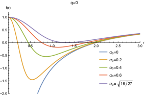
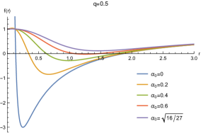
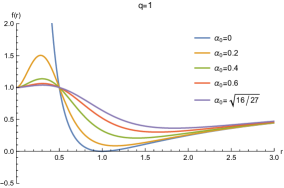
Figure 1: The metric function $f(r)$ of the Frolov BH for various $q$ and $\alpha_{0}$.

Fig.1 shows the metric function $f(r)$ of the Frolov BH for various $q$ and $\alpha_{0}$. We begin by considering the case of $q=0$, corresponding to the Hayward BH (the left plot in Fig.3). As $\alpha_{0}$ increases from the Schwarzschild BH case, the Hayward BH evolves into a BH with double horizons. Further increasing $\alpha_{0}$ to the upper bound defined by the inequality (3), the Hayward BH transforms into a BH with a single horizon. When $q\neq 0$, with an increasing $\alpha_{0}$, the Frolov geometry, initially featuring double horizons, transitions to a spacetime with a single horizon (see the second plot in Fig.1). Further increments in $\alpha_{0}$ lead to the development of a horizonless spacetime, often describing the exotic compact objects (see the second plot in Fig.1). However, when $q$ is increased to $q=1$, the Frolov geometry describes a horizonless spacetime for all $\alpha_{0}>0$ (see the right plot in Fig. 1). Fig.2 displays the phase diagram $\alpha_{0}-q$, illustrating the horizon structure of the Frolov spacetime. In this paper, we will exclusively focus on studying the case of the BH spacetime with horizons.

Figure 2: The phase diagram $\alpha_{0}-q$, illustrating the horizon structure of the Frolov spacetime.

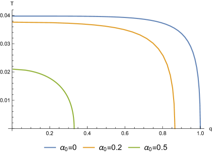
Figure 3: The Hawking temperature as a function of $q$ with different $\alpha_{0}$.

The Hawking temperature of the regular BH can be worked out as:

$$T=\frac{f^{\prime}(r_{h})}{4\pi}=\frac{r_{h}\left(-q^{2}\left(2\alpha_{0}^{2}r_{h}+r_{h}^{4}\right)-4\alpha_{0}^{2}r_{h}^{2}+r_{h}^{5}+\alpha_{0}^{2}q^{4}\right)}{2\pi\left(2\alpha_{0}^{2}r_{h}+r_{h}^{4}+\alpha_{0}^{2}q^{2}\right){}^{2}}.$$ (4)

Here, $r_{h}$ represents the event horizon of the BH. From the equation above, it’s evident that when $q=0$ and $T=0$, the upper limit of Eq. (3) is satisfied. Fig.3 illustrates the relationship between the Hawking temperature and the charge parameter $q$ for various values of $\alpha_{0}$ to aid with visualizing.

The dynamics of the probe scalar field can be described by the following Klein-Gordon (KG) equation:

$$\frac{1}{\sqrt{-g}}\partial_{\nu}(g^{\mu\nu}\sqrt{-g}\partial_{\mu}\Phi)=0\,.$$ (5)

Given the spherical symmetry of the geometry under investigation, we can employ the following spherical harmonics to separate the variables:

$$\Phi(t,r,\theta,\phi)=\sum_{l,m}Y_{l,m}(\theta,\phi)\frac{\Psi_{l,m}(t,r)}{r}\,,$$ (6)

In the above equation, $Y_{l,m}(\theta,\phi)$ is the spherical harmonics. Here, $l$ and $m$ stand for the angular and azimuthal quantum numbers, respectively. For a given $l$ and $m$, we have simplified the notation by denoting $\Psi_{l,m}(t,r)$ as $\Psi$. Then, the KG equation (5) may be reformulated in the following manner:

$$-\frac{\partial^{2}\Psi}{\partial t^{2}}+\frac{\partial^{2}\Psi}{\partial r_{\ast}^{2}}-V_{\text{eff}}\Psi=0\,,$$ (7)

where $r_{*}$ is the tortoise coordinate associated with $r$, as $\textrm{d}r_{*}/\textrm{d}r=1/f(r)$. The effective potential is given by:

$$V_{\text{eff}}=f(r)\frac{l(l+1)}{r^{2}}+\frac{f(r)f^{\prime}(r)}{r}\,,$$ (8)

with $l=0,1,\ldots$.

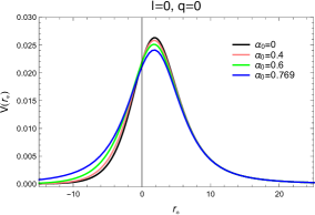
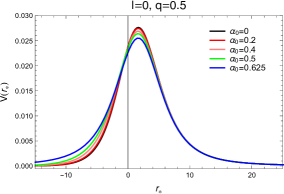
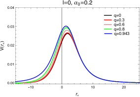
Figure 4: The effective potential $V(r_{*})$ for various BH parameter $\alpha_{0}$ and charge parameter $q$ with $l=0$.

Fig. 4 depicts the effective potential $V(r_{*})$ for different BH parameters, namely $\alpha_{0}$ and $q$, with $l=0$. For a fixed charge $q$, it is observed that as $\alpha_{0}$ increases, the peak value of the effective potential decreases, whereas the position of the peak remains almost unchanged (see the first and second plots graph in Fig.4). The third plot in Fig.4 shows the case of changing $q$ with fixed $\alpha_{0}=0.2$. With an increase in $q$, both the peak value of the effective potential and its position consistently shift to the left. Moreover, it is noteworthy that regardless of whether we vary $\alpha_{0}$ or $q$, there are discernible changes in the near-horizon behavior. These characteristics of the effective potential undoubtedly influence the behaviors of the QNMs.

III Pseudospectral Method

Numerous techniques have been devised for determining QNMs, with the pseudospectral approach being one of the potent numerical instruments. This method has been successfully applied in various models to compute QNFs, see for example Jansen:2017oag ; Wu:2018vlj ; Fu:2018yqx ; Xiong:2021cth ; Liu:2021fzr ; Liu:2021zmi ; Jaramillo:2020tuu ; Jaramillo:2021tmt ; Destounis:2021lum ; Fu:2022cul ; Fu:2023drp ; Gong:2023ghh .

We will work in the Eddington-Finkelstin coordinate system, which is advantageous for imposing the boundary conditions. Additionally, our study will be carried out in the frequency domain. To this end, we employ the following transformations:

$$r\to 1/u\ \ \text{and}\ \ \Psi=\textrm{e}^{-\textrm{i}\omega r_{*}(u)}\psi\,.$$ (9)

In the Eddington-Finkelstin coordinate system, the wave is naturally ingoing at the BH event horizon. Hence, we only need to impose the outgoing boundary condition at infinity, which is given by:

$$\psi\sim\textrm{e}^{+\textrm{i}\omega r_{*}}\,,~{}~{}~{}~{}~{}~{}\;r_{*}\rightarrow+\infty\,.$$ (10)

Collecting the equations above, the wave equation (7) is then transformed into:

$$(-l(l+1)u^{2}-2iu(1-2(1+u)f(u)+u(1+2u)f^{\prime}(u))\omega+4(1+2u)(1-f(u)$$

$$-2uf(u))\omega^{2})\psi(u)+(u^{4}f^{\prime}(u)+2iu^{2}(1-(2+4u)f(u))\omega)\psi^{\prime}(u)+u^{4}f(u)\psi^{\prime\prime}(u)=0\,,$$ (11)

where the prime represents the derivative with respect to $u$. After the transformation (9), the metric function $f(u)$ becomes

$$f(u)=1+\frac{u(-2+q^{2}u)}{1+2u^{3}\alpha_{0}^{2}+q^{2}u^{4}\alpha_{0}^{2}}\,.$$ (12)

Using the pseudospectral method to solve the eigenvalue problem in $\omega$, the pivotal step involves discretizing the wave equation (11). For more details, please refer to Ref. Jansen:2017oag . To achieve this, we employ the Chebyshev grids and Lagrange cardinal functions, defined as follows:

$$u_{i}=\cos\left(\frac{i}{N}\pi\right)\,,\ \ C_{j}(u)=\prod_{i=0,i\neq j}^{N}\frac{u-u_{i}}{u_{j}-u_{i}}\,,\ i=0\,,...\,,N\,.$$ (13)

Then, the function $\psi(u)$ can be approximated as

$$\psi(u)\approx\sum_{j=0}^{N}f(u_{j})C_{j}(u)\mathrm{,}$$ (14)

where the cardinal functions are linear combinations of Chebyshev polynomials $T_{n}(u)$ of the first kind:

$$C_{j}(u)=\frac{2}{Np_{j}}\sum_{m=0}^{N}\frac{1}{p_{m}}T_{m}(u_{j})T_{m}(u)\mathrm{~{},~{}}p_{0}=p_{N}=2\mathrm{~{},~{}}p_{j}=1\mathrm{~{}.}$$ (15)

Afterward, we can obtain the generalized eigenvalue equation in the form:

$$(M_{0}+\omega M_{1})\psi=0,$$ (16)

where $M_{i}$ ($i=0,1$) represents the linear combination of the derivative matrices $D_{ij}^{(n)}=C_{i}^{n}(u_{j})$, where $n$ represents the $n$th derivative matrix. By solving the eigenvalue function, we can determine the QNFs.

IV Quasinormal modes

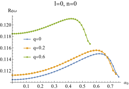
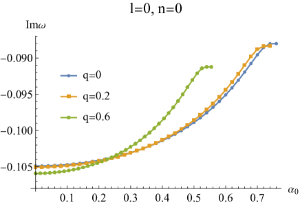
Figure 5: QNFs are presented as a function of the BH parameter $\alpha_{0}$ for different charge parameter $q$ with $l=0$ and $n=0$.

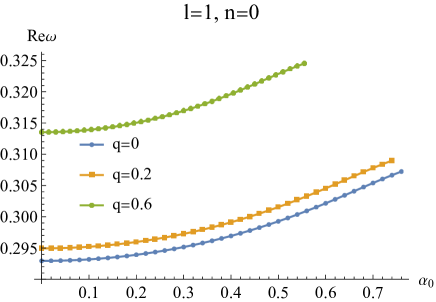
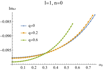
Figure 6: QNFs are presented as a function of the BH parameter $\alpha_{0}$ for different charge parameter $q$ with $l=1$ and $n=0$.

${q}$	$\omega\left(\alpha_{0}=0\right)$	$\omega\left(\alpha_{0}=1/10\right)$	$\omega\left(\alpha_{0}=1/2\right)$
$0$	0.11046 - 0.10490i	0.11061 - 0.10471i	0.11403 - 0.09889i
$2/10$	0.11124 - 0.10506i	0.11140 - 0.10486i	0.11487 - 0.09858i
$6/10$	0.11846 - 0.10593i	0.11867 - 0.10557i	0.11974 - 0.09271i

Table 1: The fundamental modes for different BH parameter $\alpha_{0}$ and charge parameter $q$ with $l=0$.

${q}$	$\omega\left(\alpha_{0}=0\right)$	$\omega\left(\alpha_{0}=1/10\right)$	$\omega\left(\alpha_{0}=1/2\right)$
$0$	0.29294 - 0.09766i	0.29318 - 0.09750i	0.29926 - 0.09287i
$2/10$	0.29494 - 0.09786i	0.29520 - 0.09769i	0.30155 - 0.09273i
$6/10$	0.31353 - 0.09915i	0.31390 - 0.09886i	0.32286 - 0.08913i

Table 2: The fundamental modes for different BH parameter $\alpha_{0}$ and charge parameter $q$ with the $l=1$.

In this section, we will explore the characteristics of the QNMs on the Frolov BH. We illustrate the behavior of the fundamental modes in relation to the BH parameter $\alpha_{0}$ for various charge parameters $q$ with $l=0$ in Fig.5 and $l=1$ in Fig.6, respectively. Additionally, for illustrative purposes, we present selected values of the fundamental modes corresponding to various BH parameters $\alpha_{0}$ and charge parameters $q$ with $l=0$ in Table 1 and $l=1$ in Table 2, respectively. It is observed that the imaginary parts consistently reside in the lower half-plane. This suggests that the Frolov BH remains stable when subjected to scalar perturbations.

Now, we will delve deeper into studying some particular characteristics of the QNFs for the fundamental modes with respect to both the BH parameter $\alpha_{0}$ and the charge parameter $q$. When $l=0$, there is a clear non-monotonic pattern in the real parts of QNFs with respect to the BH parameter $\alpha_{0}$ for a given value of $q$ (see the left plot in Fig.5). The phenomenon of non-monotonic behavior has been documented in LQG-corrected BH, as reported in the works of Fu:2023drp ; Gong:2023ghh . To be more precise, as an increase in the parameter $\alpha_{0}$, signifying the system is farther from the Schwarzschild BH or the RN BH, the real parts of the QNFs initially go up, which means that the system is oscillating more strongly, and then it goes down, which means that the oscillation is weakening. As the charge parameter $q$ goes up, the turning point of this non-monotonic behavior goes down. It is important to note that the real parts are smaller than that of the Schwarzschild BH or the RN BH as the parameter $\alpha_{0}$ increases. At the same time, as $\alpha_{0}$ goes up, so do the values of the imaginary parts of the QNFs, which points to a lower damping rate (see the right plot in Fig.5). This result suggests that when quantum gravity effects are present, we have a slower decay modes.

Furthermore, if we fix the BH parameter $\alpha_{0}$, we observe that in the region of small $\alpha_{0}$, the real parts of QNFs increase as the charge parameter $q$ rises, indicating that the charge enhances the oscillation of the system. As the parameter $\alpha_{0}$ increases, we observe that the curves with $q=0.2$ and $q=0.6$ intesect (see the left plot in Fig.5), suggesting an opposite trend in the change with $q$. The opposite change trend with $q$ between small $\alpha_{0}$ and large $\alpha_{0}$ is more pronounced in the imaginary parts (see the right plot in Fig.5). We also observe that when $\alpha_{0}$ is relatively large, the curves intersect again.

Next, we examine the scenario when $l=1$ in detail, as shown in Fig.6. The non-monotonic behavior ceases to exist at $l=1$. Specifically, both the real and imaginary parts consistently and continuously go up as the parameter $\alpha_{0}$ goes up. This means that the system oscillates more strongly and decays more slowly. we also do an analysis of the QNFs for the values of $l>1$ and arrive at a similar result as in the case when $l=1$. An analogous discovery has been documented with the fundamental modes of the LQG-corrected BH Gong:2023ghh . This means that the angular number has a bigger effect on the fundamental modes than quantum gravity effects. Further research should be done in the future into the universality of the non-monotonic behavior for $l=0$ and a study into the reasons behind this phenomenon.

V Ringdown waveform

In this section, we will investigate the time-domain profiles of the scalar field over the Frolov BH. To do this, we need to solve numerically the time-dependent wave equation (7) using the following initial Gaussian wave packet:

$$\Psi(r_{*},t=0)=\exp\left[{-\frac{(r_{*}-a)^{2}}{2b^{2}}}\right]\,,\$$

$$\Psi(r_{*},t<0)=0\,.$$ (17)

Without loss of generality, we fix the tortoise coordinate at $r_{*}=5$. Notes that, the different of initial conditions (17) can not influence the ringdown waveform. After the initial outburst stage, the ringdown waveform is fully determine by the QNMs, also called the quasinormal ringing stage.

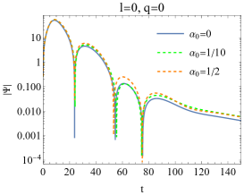
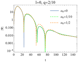
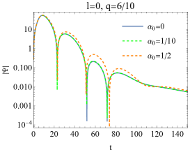
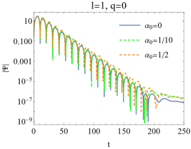
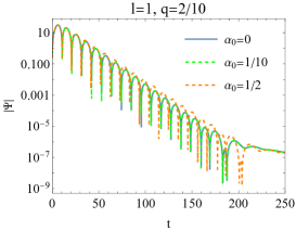
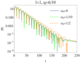
Figure 7: The semilogarithmic plots of the time-domain profiles of scalar field for $l=0$ and $l=1$ with different parameters of $q$ and $\alpha_{0}$.

In Fig.7 , we display the semilogarithmic plots of the time-domain evolution of the scalar field for $l=0$ and $l=1$, showcasing various combinations of $q$ and $\alpha_{0}$ parameters. Notably, there is no increase in perturbation over time. Furthermore, we conduct a fitting analysis on the late-time tail decay, revealing a power-law behavior represented as $\Psi\sim t^{-2l+3}$. These findings provide additional confirmation that the Frolov BH is dynamic stability when subjected to perturbations from a massless scalar field. This observation aligns with the findings from QNMs. Additionally, as a validation check, we employ the Prony method to fit the fundamental mode, presenting the results in Table 3 and 4. These findings align with those obtained through the pseudospectral method, as presented in Table 1 and 2.

${q}$	$\omega\left(\alpha_{0}=0\right)$	$\omega\left(\alpha_{0}=1/10\right)$	$\omega\left(\alpha_{0}=1/2\right)$
$0$	0.11089 - 0.10049i	0.11401 - 0.096998i	0.11534 - 0.092569i
$2/10$	0.11462 - 0.09729i	0.11469 - 0.097132i	0.11598 - 0.092354i
$6/10$	0.11160 - 0.10301i	0.11781 - 0.098063i	0.11852 - 0.086906i

Table 3: The fundamental modes obtained by the Prony method for different BH parameter $\alpha_{0}$ and charge parameter $q$ with the $l=0$.

${q}$	$\omega\left(\alpha_{0}=0\right)$	$\omega\left(\alpha_{0}=1/10\right)$	$\omega\left(\alpha_{0}=1/2\right)$
$0$	0.29287 - 0.097679i	0.29301 - 0.097522i	0.29917 - 0.092926i
$2/10$	0.29478 - 0.097902i	0.29504 - 0.097735i	0.30146 - 0.092794i
$6/10$	0.31350 - 0.099311i	0.31387 - 0.099015i	0.32288 - 0.089244i

Table 4: The fundamental modes obtained by the Prony method for different BH parameter $\alpha_{0}$ and charge parameter $q$ with the $l=1$.

VI Conclusions and discussions

In this paper, we have investigated the properties of QNMs of the scalar field over the Frolov BH and have also provided a brief discussion on its time-domain evolution. The Frolov BH exhibits stability against scalar perturbations, as evidenced by the consistent residence of the imaginary parts of the QNMs in the lower half-plane and the gradual decay of perturbations over time.

When the angular quantum number $l=0$, the real parts of QNFs display distinct non-monotonic behaviors. Specifically, with an increase in the BH parameter $\alpha_{0}$, the system undergoes stronger oscillations initially, followed by a weakening. The turning point of this non-monotonic behavior shifts downward as the charge parameter $q$ increases. Furthermore, as the parameter $\alpha_{0}$ increases, the real parts become smaller compared to those of the Schwarzschild BH or the RN BH. This suggests that at this moment, the system undergoes weaker oscillations than the Schwarzschild BH or the RN BH. While the BH parameter $\alpha_{0}$ contributes to reducing the damping rate, as indicated by the increase in the values of the imaginary parts of the QNFs as $\alpha_{0}$ rises. This outcome suggests that the presence of quantum gravity effects leads to slower decay modes. We also briefly explore the impact of the charge parameter $q$. The study indicates that the charge enhances the oscillations of the system. In addition, upon examining scenarios with higher angular quantum numbers ($l\geq 1$), we observe the disappearance of the non-monotonic behavior observed in the case of $l=0$. This disappearance may be attributed to the influence of the angular quantum number outweighing that of the quantum gravity effect. Further research is warranted to explore the universality of the non-monotonic behavior for $l=0$.

- (1) J. Bardeen, Non-singular general-relativistic gravitational collapse, in Proceedings of the International Conference GR5,Tbilisi,USSR,P.174. Tbilisi University Press (1968).
- (2) S. A. Hayward, Formation and evaporation of regular black holes, Phys. Rev. Lett. 96 (2006) 031103, [gr-qc/0506126].
- (3) V. P. Frolov, Notes on nonsingular models of black holes, Phys. Rev. D 94 (2016), no. 10 104056, [arXiv:1609.01758].
- (4) L. Xiang, Y. Ling, and Y. G. Shen, Singularities and the Finale of Black Hole Evaporation, Int. J. Mod. Phys. D 22 (2013) 1342016, [arXiv:1305.3851].
- (5) H. Culetu, On a regular modified Schwarzschild spacetime, arXiv:1305.5964.
- (6) H. Culetu, On a regular charged black hole with a nonlinear electric source, Int. J. Theor. Phys. 54 (2015), no. 8 2855–2863, [arXiv:1408.3334].
- (7) M. E. Rodrigues, E. L. B. Junior, G. T. Marques, and V. T. Zanchin, Regular black holes in gravity coupled to nonlinear electrodynamics, Phys. Rev. D 94 (2016), no. 2 024062, [arXiv:1511.00569]. [Addendum: Phys.Rev.D 94, 049904 (2016)].
- (8) A. Simpson and M. Visser, Regular black holes with asymptotically Minkowski cores, Universe 6 (2019), no. 1 8, [arXiv:1911.01020].
- (9) S. G. Ghosh, A nonsingular rotating black hole, Eur. Phys. J. C 75 (2015), no. 11 532, [arXiv:1408.5668].
- (10) S. G. Ghosh, D. V. Singh, and S. D. Maharaj, Regular black holes in Einstein-Gauss-Bonnet gravity, Phys. Rev. D 97 (2018), no. 10 104050.
- (11) X. Li, Y. Ling, Y.-G. Shen, C.-Z. Liu, H.-S. He, and L.-F. Xu, Generalized uncertainty principles, effective Newton constant and the regular black hole, Annals Phys. 396 (2018) 334–350, [arXiv:1611.09016].
- (12) M. Martinis and N. Perkovic, Is exponential metric a natural space-time metric of Newtonian gravity?, arXiv:1009.6017.
- (13) Y. Ling and M.-H. Wu, Regular black holes with sub-Planckian curvature, Class. Quant. Grav. 40 (2023), no. 7 075009, [arXiv:2109.05974].
- (14) C. Bambi, Regular Black Holes. Springer Series in Astrophysics and Cosmology. Springer Singapore, 2023.
- (15) S. Vagnozzi et al., Horizon-scale tests of gravity theories and fundamental physics from the Event Horizon Telescope image of Sagittarius A, Class. Quant. Grav. 40 (2023), no. 16 165007, [arXiv:2205.07787].
- (16) C. Lan, H. Yang, Y. Guo, and Y.-G. Miao, Regular Black Holes: A Short Topic Review, Int. J. Theor. Phys. 62 (2023), no. 9 202, [arXiv:2303.11696].
- (17) E. Berti, V. Cardoso, and A. O. Starinets, Quasinormal modes of black holes and black branes, Class. Quant. Grav. 26 (2009) 163001, [arXiv:0905.2975].
- (18) E. Berti, V. Cardoso, and C. M. Will, On gravitational-wave spectroscopy of massive black holes with the space interferometer LISA, Phys. Rev. D 73 (2006) 064030, [gr-qc/0512160].
- (19) E. Berti, K. Yagi, H. Yang, and N. Yunes, Extreme Gravity Tests with Gravitational Waves from Compact Binary Coalescences: (II) Ringdown, Gen. Rel. Grav. 50 (2018), no. 5 49, [arXiv:1801.03587].
- (20) G. Fu, D. Zhang, P. Liu, X.-M. Kuang, Q. Pan, and J.-P. Wu, Quasinormal modes and Hawking radiation of a charged Weyl black hole, Phys. Rev. D 107 (2023), no. 4 044049, [arXiv:2207.12927].
- (21) G. Fu, D. Zhang, P. Liu, X.-M. Kuang, and J.-P. Wu, Peculiar properties in quasinormal spectra from loop quantum gravity effect, Phys. Rev. D 109 (2024), no. 2 026010, [arXiv:2301.08421].
- (22) H. Gong, S. Li, D. Zhang, G. Fu, and J.-P. Wu, Quasinormal modes of quantum-corrected black holes, arXiv:2312.17639.
- (23) L. A. Lopez and V. Hinojosa, Quasinormal modes of Charged Regular Black Hole, Can. J. Phys. 99 (2021), no. 1 44–48, [arXiv:1810.09034].
- (24) A. Jansen, Overdamped modes in Schwarzschild-de Sitter and a Mathematica package for the numerical computation of quasinormal modes, Eur. Phys. J. Plus 132 (2017), no. 12 546, [arXiv:1709.09178].
- (25) J.-P. Wu and P. Liu, Quasi-normal modes of holographic system with Weyl correction and momentum dissipation, Phys. Lett. B 780 (2018) 616–621, [arXiv:1804.10897].
- (26) G. Fu and J.-P. Wu, EM Duality and Quasinormal Modes from Higher Derivatives with Homogeneous Disorder, Adv. High Energy Phys. 2019 (2019) 5472310, [arXiv:1812.11522].
- (27) W. Xiong, P. Liu, C.-Y. Zhang, and C. Niu, Quasi-normal modes of the Einstein-Maxwell-aether Black Hole, arXiv:2112.12523.
- (28) P. Liu, C. Niu, and C.-Y. Zhang, Linear instability of charged massless scalar perturbation in regularized 4D charged Einstein-Gauss-Bonnet anti de-Sitter black holes, Chin. Phys. C 45 (2021), no. 2 025111.
- (29) P. Liu, C. Niu, and C.-Y. Zhang, Instability of regularized 4D charged Einstein-Gauss-Bonnet de-Sitter black holes, Chin. Phys. C 45 (2021), no. 2 025104.
- (30) J. L. Jaramillo, R. Panosso Macedo, and L. Al Sheikh, Pseudospectrum and Black Hole Quasinormal Mode Instability, Phys. Rev. X 11 (2021), no. 3 031003, [arXiv:2004.06434].
- (31) J. L. Jaramillo, R. Panosso Macedo, and L. A. Sheikh, Gravitational wave signatures of black hole quasi-normal mode instability, arXiv:2105.03451.
- (32) K. Destounis, R. P. Macedo, E. Berti, V. Cardoso, and J. L. Jaramillo, Pseudospectrum of Reissner-Nordström black holes: Quasinormal mode instability and universality, Phys. Rev. D 104 (2021), no. 8 084091, [arXiv:2107.09673].