Bayesian inference for spatial-temporal non-Gaussian data using predictive stacking

Abstract.

Analysing non-Gaussian spatial-temporal data typically requires introducing spatial dependence in generalised linear models through the link function of an exponential family distribution. However, unlike in Gaussian likelihoods, inference is considerably encumbered by the inability to analytically integrate out the random effects and reduce the dimension of the parameter space. Iterative estimation algorithms struggle to converge due to the presence of weakly identified parameters. We devise an approach that obviates these issues by exploiting generalised conjugate multivariate distribution theory for exponential families, which enables exact sampling from analytically available posterior distributions conditional upon some fixed process parameters. More specifically, we expand upon the Diaconis-Ylvisaker family of conjugate priors to achieve analytically tractable posterior inference for spatially-temporally varying regression models conditional on some kernel parameters. Subsequently, we assimilate inference from these individual posterior distributions over a range of values of these parameters using Bayesian predictive stacking. We evaluate inferential performance on simulated data, compare with fully Bayesian inference using Markov chain Monte Carlo and apply our proposed method to analyse spatially-temporally referenced avian count data from the North American Breeding Bird Survey database.

Keywords. Bayesian inference; Generalised linear models; Predictive stacking; Spatial-temporal models.

1. Introduction

Statistical modelling and analysis for spatially oriented non-Gaussian outcomes play a crucial role in diverse scientific applications (see, for example, De Oliveira et al., 1997; Diggle et al., 1998; Heagerty and Lele, 1998; De Oliveira, 2000; Zhang et al., 2022; Saha et al., 2022). Diverse scientific investigations involve spatially, and possibly temporally, oriented outcomes that are not Gaussian, or even continuous. For example, climate scientists record daily or monthly binary variables at spatial locations indicating whether, or not, rainfall was measurable; ecologists and forest scientists analyse temporal evolution of species counts at locations; and economists study the spatial distribution of the number of insurance claims at different locations over time. While spatial-temporal count data are sometimes aggregated into rates or counts over larger regions, statisticians are increasingly encountering count data referenced by space-time coordinates.

For our purposes, we consider a spatial-temporal process as an uncountable set of random variables, say $\{z(\ell):\ell\in\mathcal{D}\}$, over a domain of interest $\mathcal{D}$, which is endowed with a probability law specifying the joint distribution for any finite sample from that set. In spatial-temporal settings $\mathcal{D}=\mathcal{S}\times\mathcal{T}$, where $\mathcal{S}\subset\mathbb{R}^{d}$ is the spatial region, $\mathcal{T}\subset[0,\infty)$ is the time domain and $\ell=(s,t)$ is a space-time coordinate with spatial location $s\in\mathcal{S}$ and time point $t\in\mathcal{T}$ (see, e.g., Gneiting and Guttorp, 2010, for a review). Following Diggle et al. (1998), we introduce spatial-temporal stochastic processes for non-Gaussian data. Let $y(\ell)$ be the outcome at $\ell$ endowed with a probability law from the natural exponential family, which we denote by

$$y(\ell)\sim\mathrm{EF}(x(\ell)^{\top}\beta+z(\ell);b,\psi_{y})$$ (1)

for some positive parameter $b>0$ and unit log partition function $\psi_{y}$ (Section 2.1). Fixed effects regression and spatial dependence, e.g., $x(\ell)^{{\top}}\beta+z(\ell)$, is introduced in the natural parameter, where $x(\ell)$ is a $p\times 1$ vector of predictors referenced with respect to $\ell$, $\beta$ is a $p\times 1$ vector of slopes measuring the trend, $z(\ell)$ is a zero-centred spatial-temporal process on $\mathbb{R}^{d}$ specified by a scale parameter $\sigma_{z}$ and a spatial correlation function $R(\cdot,\cdot;{\theta_{\text{sp}}})$ with ${\theta_{\text{sp}}}$ consisting of spatial-temporal decay and smoothness parameters. This structure is embodied by spatial generalised mixed-effect models (McCulloch and Searle, 2001; Hughes and Haran, 2013). Bayesian inference for (1) is appealing as it offers fully probabilistic inference for the latent process. However, the presence of $z(\ell)$ presents challenges for non-Gaussian families as we cannot integrate out $z$, which begets a high-dimensional parameter space. Iterative algorithms such as Markov Chain Monte Carlo (MCMC) attempt to sample from the posterior distribution, but convergence is often hampered by high auto-correlations and weakly identified parameters ${\theta_{\text{sp}}}$. Section 1.3 in Haran (2011) offers a detailed overview of MCMC algorithms for estimating such models.

Rather than devising computational algorithms to achieve improved convergence, we develop a framework to conduct Bayesian inference for fixed effects and the latent spatial-temporal process by entirely avoiding convergence issues for MCMC or other iterative algorithms for spatial-temporal non-Gaussian data. Instead, we build a hierarchical model that yields analytically accessible posterior distributions for $\beta$ and $z$ subject to fixing weakly identified parameters ${\theta_{\text{sp}}}$ and some hyper-parameters so that we can draw exact posterior samples for any fixed values of these parameters. This is achieved by availing of recent results developed in Bradley and Clinch (2024) on a new class of analytically accessible conjugate multivariate ($\mathrm{CM}$) and generalised conjugate multivariate ($\mathrm{GCM}$) distributions for spatial models by extending the Diaconis-Ylvisaker family of conjugate priors for exponential families (Diaconis and Ylvisaker, 1979). Our current manuscript expands significantly over this framework. Not only do we move from spatial to spatial-temporal processes, we further enrich (1) by introducing spatially-temporally varying regression coefficients (Gelfand et al., 2003). Such models are attractive in the Bayesian paradigm as they capture the impact of explanatory variables or predictors over space and time and offer inference on processes that are completely unobserved. However, these extensions are not straightforward because of the presence of explanatory variables in the fixed regression component and also in a spatially-temporally varying component.

The literature on spatially-temporally varying coefficient models is rather sparse and has remained purely notional for exponential families, perhaps because they require extensive tuning of MCMC or other iterative algorithms that struggle with weakly identified parameters and high-dimensional random effects. Hence, we devise Bayesian predictive stacking for estimating such models. Stacking (Wolpert, 1992; Breiman, 1996; Clyde and Iversen, 2013) is a model averaging procedure that is widely used in machine learning and has been shown (see, e.g., Le and Clarke, 2017; Yao et al., 2018, 2020, 2021) to be an effective alternative to traditional Bayesian model averaging (Madigan et al., 1996; Hoeting et al., 1999). Let $\mathcal{M}=\{M_{1},\dots,M_{L}\}$ denote a collection of $L$ candidate models, where each $M_{l}$ corresponds to a fixed set of values of certain parameters (${\theta_{\text{sp}}}$ and, for our subsequent development, a boundary adjustment parameter) that allow us to exactly sample from the posterior distributions $p_{l}(\beta,z\mid y)$ for $l=1,\ldots,L$. Rather than pursuing full inference using iterative sampling algorithms, we offer inference by “stacking” these $L$ posterior distributions by solving for the optimal set of weights needed to calculate the weighted average of the $L$ analytically available posterior distributions. Bayesian model averaging asymptotically chooses a single model in $\mathcal{M}$ that is closest to an oracle $M_{0}$ in terms of Kullback-Leibler divergence and, hence, is appropriate if $\mathcal{M}$ contains the true data generating model $M_{0}$, but is flawed otherwise. Yao et al. (2018) adapts stacking to assimilate different Bayesian predictive distributions and appears more tenable in practical geostatistics (Zhang et al., 2023).

After briefly discussing $\mathrm{CM}$ and $\mathrm{GCM}$ distributions with multivariate extensions in Section 2, Section 3 introduces our hierarchical spatially-temporally varying regression model and derives accessible posterior distributions. Section 4 develops predictive stacking with novel results on posterior sampling and predictive inference. Sections 5 and 6 present simulation experiments demonstrating the effectiveness of our method and analyses a spatial-temporal dataset on avian counts. We conclude with some discussion and directions for future work in Section 7.

2. Conjugate priors for exponential family

2.1. The Diaconis-Ylvisaker distribution

Let $Y$ be distributed from the natural exponential family, $\mathrm{EF}(\eta;b,\psi)$, with density

$$p(Y\mid\eta)=\exp\{\eta Y-b\psi(\eta)+c(Y)\},\ Y\in\mathscr{Y},\eta\in\mathscr{H}\;,$$ (2)

where $\mathscr{Y}$ denotes the support of $Y$ and $\mathscr{H}=\{\eta:\psi(\eta)<\infty\}$ denotes the natural parameter space and, therefore, the support of $\eta$. The scalar $b$ may be unknown, while $\psi(\cdot)$ and $c(\cdot)$ are known functions. We will be discussing various forms of the unit log partition function $\psi(\cdot)$ and the scalar $b$ to denote different distributions from the family. Diaconis and Ylvisaker (1979) provides a proper conjugate prior for $\eta$ in (2) as $\mathrm{DY}(\alpha,\kappa;\psi)$, which has the density

$$p(\eta\mid\alpha,\kappa)\propto\exp\{\alpha\eta-\kappa\psi(\eta)\},\ \eta\in\mathscr{H},\frac{\alpha}{\kappa}\in\mathscr{Y},\kappa>0\;.$$ (3)

It is easily seen that the posterior distribution $\eta\mid Y,\alpha,\kappa\sim\mathrm{DY}(\alpha+Y,\kappa+b;\psi)$. There are several special cases of the $\mathrm{DY}$ distribution other than the Gaussian ($\psi=\psi_{1}$), log-gamma ($\psi=\psi_{2}$), and logit-beta ($\psi=\psi_{3}$) distributions, several of which do not correspond to a member of the exponential family. For example, $\alpha=0$, $\psi(t)=\psi_{4}(t)=\log(1+t^{2}/\nu)$, and $\kappa=(\nu+1)/2$ with $\nu>0$ results in a Student’s $t$-distribution with $\nu$ degrees of freedom.

2.2. The (Generalised) Conjugate Multivariate distribution

Bradley et al. (2020) introduced a multivariate version of (3) using linear combinations of mutually independent DY random variables. Let $\zeta$ be the $n\times 1$ random vector

$$\zeta=\mu+L\eta\;,$$ (4)

where $\zeta\in\mathscr{M}$, $\mathscr{M}=\{\zeta:\zeta=\mu+L\eta,\eta\in\mathscr{H}^{n}\}$, $\mu\in\mathbb{R}^{n}$ denotes a location vector, $L$ is an $n\times n$ lower-triangular matrix with positive diagonal elements and the $n\times 1$ random vector $\eta=(\eta_{1},\dots,\eta_{n})^{\top}$ consists of $n$ mutually independent DY random variables, $\eta_{i}\sim\mathrm{DY}(\alpha_{i},\kappa_{i};\psi)$ with $\kappa_{i}>0$ for $i=1,\dots,n$. Define $\zeta\sim\mathrm{CM}(\mu,L,\alpha,\kappa;\psi)$ with unnormalised density

$$p(\zeta\mid\mu,L,\alpha,\kappa)\propto\exp\left\{\alpha^{\top}L^{-1}(\zeta-\mu)-\kappa^{\top}\psi(L^{-1}(\zeta-\mu))\right\}\det(L^{-1})$$ (5)

for all $\zeta\in\mathscr{M}$, where $\psi$ operates element-wise on $L^{-1}(\zeta-\mu)$, $\alpha=(\alpha_{1},\dots,\alpha_{n})^{\top}$ and $\kappa=(\kappa_{1},\dots,\kappa_{n})^{\top}$. If $\zeta=(\zeta_{1}^{\top},\zeta_{2}^{\top})^{\top}$ is distributed as $\mathrm{CM}(\mu,L,\alpha,\kappa;\psi)$, where $\zeta_{1}$ is $r\times 1$ and $\zeta_{2}$ is $(n-r)\times 1$, then the conditional distribution of $\zeta_{1}$ given $\zeta_{2}$ is $\mathrm{CM_{c}}(\mu^{*},A_{1},\alpha,\kappa;\psi)$ with

$$p(\zeta_{1}\mid\zeta_{2}=c_{2},\mu^{*},A_{1},\alpha,\kappa)\propto\exp\{\alpha^{\top}(A_{1}\zeta_{1}-\mu^{*})-\kappa^{\top}\psi(A_{1}\zeta_{1}-\mu^{*})\}\;,$$ (6)

as the unnormalised density for all $(\zeta_{1}^{\top},c_{2}^{\top})^{\top}\in\mathscr{M}$. Here, $A_{1}$ is defined as the $n\times r$ submatrix of $L^{-1}=[A_{1}:A_{2}]$, and $\mu^{*}=L^{-1}\mu-A_{2}c_{2}$ for some $c_{2}\in\mathbb{R}^{n-r}$. The proportionality constant in (6) is strictly positive and finite ensuring that (6) is proper (Bradley et al., 2020).

Bradley and Clinch (2024) generalise the $\mathrm{CM}$ distribution by relating $\zeta$, $\mu$, $L$ and $\eta$ as in (4), where $\zeta=(\zeta_{1}^{\top},\dots,\zeta_{K}^{\top})^{\top}$ and $\eta=(\eta_{1}^{\top},\dots,\eta_{K}^{\top})^{\top}$ are $n\times 1$ with $n=\sum_{k=1}^{K}n_{k}$, and each element of $\eta_{k}$ is independently distributed as $\eta_{k,i}\sim\mathrm{DY}(\alpha_{k,i},\kappa_{k,i};\psi_{k})$, $L$ is an $n\times n$ lower-triangular matrix with positive diagonal elements and $\mu$ is an $n\times 1$ location parameter. The density is written analogously to (5) with $\zeta\in\mathscr{N}$, $\mathscr{N}=\{\zeta:\zeta=\mu+L\eta,\eta_{k,i}\in\mathscr{H}_{k},i=1,\dots,n_{k},k=1,\dots,K\}$ with $\mathscr{H}_{k}$ being the parameter space corresponding to the log partition function $\psi_{k}$, $\alpha_{k,i}/\kappa_{k,i}\in\mathscr{Y}_{k}$, $\kappa_{k,i}>0$ and $\psi(L^{-1}(\zeta-\mu))=(\psi_{1}(J_{1}L^{-1}(\zeta-\mu))^{\top},\dots,\psi_{K}(J_{K}L^{-1}(\zeta-\mu))^{\top})^{\top}$, where $J_{k}=[0:I_{n_{k}}:0]$ is $n_{k}\times n$ and each $\psi_{k}(\cdot)$ operates element-wise on the vector of arguments, $\alpha=(\alpha_{1}^{\top},\dots,\alpha_{K}^{\top})^{\top}$ and $\kappa=(\kappa_{1}^{\top},\dots,\kappa_{K}^{\top})^{\top}$ are $n\times 1$ parameter vectors.

We say $\zeta$ is distributed as $\mathrm{GCM}(\mu,L,\alpha,\kappa;\psi)$. A conditional $\mathrm{GCM}$ density up to a normalising constant is obtained analogous to (6) and denoted as $\mathrm{GCM_{c}}(\mu^{*},A_{1},\alpha,\kappa;\psi)$. We use these distributions for building the hierarchical models in the following sections. In general, we may be unable to sample directly from either the conditional $\mathrm{CM}$ or the conditional $\mathrm{GCM}$ distributions except for some familiar exceptions (e.g., the conditional distribution of Gaussian is indeed Gaussian). However, it is possible to consider an augmented model with a particular structure that yields a posterior distribution in the $\mathrm{GCM}$ family that is easy to sample from (Section 3).

3. Bayesian hierarchical model

3.1. Conjugate spatial-temporal process

The prevalent specification for $z(\ell)$ in (1) is a Gaussian process. This is a special case of a “$\mathrm{CM}$” process ($\mathrm{CMP}$) on $\mathcal{D}$. We write $z(\ell)\sim\mathrm{CMP}(\mu_{z}(\ell),\allowbreak V_{z}(\cdot,\cdot),\alpha_{z},\kappa_{z};\psi_{z})$ if, for any finite collection $\mathcal{L}=\{\ell_{1},\dots,\ell_{n}\}\subset\mathcal{D}$, the $n\times 1$ vector $z(\mathcal{L})=(z(\ell_{1}),\dots,z(\ell_{n}))^{\top}$ is distributed as $\mathrm{CM}(\mu_{z}(\mathcal{L}),L_{z},\alpha_{z},\kappa_{z};\psi_{z})$, $\mu_{z}(\mathcal{L})=(\mu_{z}(\ell_{1}),\dots,\mu_{z}(\ell_{n}))^{\top}$ and $L_{z}$ is the lower-triangular Cholesky factor of the $n\times n$ matrix $V_{z}(\mathcal{L};\theta)=(V_{z}(\ell_{i},\ell_{j};\theta))$ for $i,j=1,\ldots,n$ and $V_{z}(\ell,\ell^{\prime};\theta)$ is a spatial covariance function indexed by parameters $\theta$. The $\mathrm{CM}$ process endows a $\mathrm{CM}$ distribution on $\{z(\ell):\ell\in\mathcal{L}\}$, thereby enabling predictive inference over the entire domain $\mathcal{D}$ based on partial realisations of the process. The Gaussian process is a $\mathrm{CM}$ process with $\psi_{z}=\psi_{1}$. A crucial extension here is to move from the real-valued process in (1) to a vector-valued process $z(\ell)$ with each element following a $\mathrm{CM}$ process. This vector-valued process is composed of univariate spatial-temporal process that model regression coefficients for certain predictors whose impact is posited to vary over space and time. We elaborate below.

3.2. Conjugate Bayesian spatially-temporally varying coefficients model

Let $\mathcal{L}=\{\ell_{1},\allowbreak\ldots,\ell_{n}\}$ be a fixed set of $n$ distinct space-time coordinates in $\mathcal{D}$, where $y(\mathcal{L})=(y(\ell_{1}),\dots,y(\ell_{n}))^{\top}\in\mathscr{Y}^{n}$, which we simply denote by $y$, is the vector of observed outcomes. We introduce spatially-temporally varying coefficients as

$$\begin{split}y(\ell_{i})\mid\beta,z(\ell_{i}),\xi_{i},\mu_{i}&\overset{\text{ind.}}{\sim}\mathrm{EF}\left(x(\ell_{i})^{\top}\beta+\tilde{x}(\ell_{i})^{{\top}}z(\ell_{i})+\xi_{i}-\mu_{i};b,\psi_{y}\right),\quad(i=1,\dots,n)\\ z_{j}\mid\sigma_{z_{j}},L_{z_{j}},\alpha_{z},\kappa_{z}&\overset{\text{ind.}}{\sim}\mathrm{CM}(\mu_{z_{j}},\sigma_{z_{j}}L_{z_{j}}({\theta_{\text{sp}}}_{j}),\alpha_{z_{j}},\kappa_{z_{j}};\psi_{z_{j}}),\quad(j=1,\dots,r)\\ \beta\mid\sigma_{\beta},L_{\beta},\alpha_{\beta},\kappa_{\beta}&\sim\mathrm{CM}(\mu_{\beta},\sigma_{\beta}L_{\beta},\alpha_{\beta},\kappa_{\beta};\psi_{\beta})\\ \xi\mid\beta,z,\mu,\sigma_{\xi},\alpha_{\xi},\kappa_{\xi}&\sim\mathrm{GCM_{c}}(\tilde{\mu}_{\xi},H_{\xi},\alpha_{\xi},\kappa_{\xi};\psi_{\xi}),\quad\theta\sim\pi(\theta)\;,\end{split}$$ (7)

where $x(\ell_{i})$ is a $p\times 1$ vector of predictors, $\beta$ is the corresponding $p\times 1$ vector of slopes (fixed effects), $\tilde{x}(\ell_{i})$ is the $r\times 1$ vector ($r\leq p$) consisting of those predictors in $x(\ell_{i})$ that are posited to have spatially varying regression coefficients, and $z_{j}=(z_{j}(\ell_{1}),\ldots,z_{j}(\ell_{n}))^{{\top}}$ is $n\times 1$ with each $z_{j}(\ell_{i})$ being a spatially-temporally varying coefficient for the predictor $\tilde{x}_{j}(\ell_{i})$.

For subsequent developments, we assume that the probability law of the $nr\times 1$ vector $z=(z_{1}^{{\top}},\ldots,z_{r}^{{\top}})^{{\top}}$ is derived by assuming that $z_{j}(\ell)\overset{\text{ind.}}{\sim}\mathrm{CMP}(\mu_{z_{j}}(\ell),\sigma_{z_{j}}^{2}R_{j}(\cdot,\cdot;{\theta_{\text{sp}}}_{j}))$ are a collection of $r$ independent $\mathrm{CM}$ processes with their respective parameters and log partition functions. The spatial covariance matrix for $z_{j}$ is given by $\sigma_{z_{j}}^{2}L_{z}({\theta_{\text{sp}}}_{j})L_{z}({\theta_{\text{sp}}}_{j})^{{\top}}$, where $\sigma_{z_{j}}^{2}$ is the spatial variance corresponding to process $z_{j}(\ell)$ and $L_{z}({\theta_{\text{sp}}}_{j})$ is the lower-triangular Cholesky factor of an $n\times n$ spatial correlation matrix $R_{j}({\theta_{\text{sp}}}_{j})$. We model the elements of $R_{j}({\theta_{\text{sp}}}_{j})$ using the spatial-temporal correlation function (see, e.g., Gneiting and Guttorp, 2010, for other examples)

$$R_{j}(\ell,\ell^{\prime};{\theta_{\text{sp}}}_{j})=\frac{1}{\phi_{1j}|t-t^{\prime}|^{2}+1}\exp\left(-\frac{\phi_{2j}\|s-s^{\prime}\|}{\sqrt{1+\phi_{1j}|t-t^{\prime}|^{2}}}\right),\quad\phi_{1j},\phi_{2j}>0\;,$$ (8)

where $\ell=(s,t)$ and $\ell^{\prime}=(s^{\prime},t^{\prime})$ are any two distinct space-time coordinates in $\mathcal{D}$, $\|\cdot\|$ is the Euclidean distance over $\mathcal{S}$, ${\theta_{\text{sp}}}_{j}=(\phi_{1j},\phi_{2j})$, and $\phi_{1j}$ and $\phi_{2j}$ are positive spatial and temporal decay parameters, respectively. For ease of notation, we drop ${\theta_{\text{sp}}}_{j}$ in (8) and simply write $R_{j}(\cdot,\cdot)$ for the correlation function. The specification for each $z_{j}(\ell)$ is completed with $\mathrm{CM}$ distribution parameters $\alpha_{z_{j}}$, $\kappa_{z_{j}}$ and $\psi_{z_{j}}$, all specific to the $j$th process.

The prior for $\beta$ is also a $\mathrm{CM}$ distribution with parameters defined analogously and the variance-covariance parameter $\sigma_{\beta}^{2}L_{\beta}L_{\beta}^{{\top}}$, where $L_{\beta}$ is the Cholesky factor of a fixed correlation matrix $V_{\beta}$. The conditional prior for $\xi$ is a $\mathrm{GCM_{c}}$ distribution with the $2n\times n$ matrix $H_{\xi}=[I_{n}:\sigma_{\xi}I_{n}]^{\top}$, location parameter $\tilde{\mu}_{\xi}=H_{\xi}((\mu-X\beta-\tilde{X}z)^{\top},\mu_{\xi}^{\top})^{\top}$, where $\mu=(\mu_{1},\ldots,\mu_{n})^{\top}$ is $n\times 1$, shape and scale parameters $\alpha_{\xi}=(\alpha_{\epsilon}1_{n}^{\top},0_{n}^{\top})^{\top}$ and $\kappa_{\xi}=(\kappa_{\epsilon}1_{n}^{\top},(1/2)1_{n}^{\top})^{\top}$, respectively, for some fixed positive reals $\alpha_{\epsilon}$ and $\kappa_{\epsilon}$. The unit log partition function $\psi_{\xi}$ is defined as $\psi_{\xi}(h)=(\psi_{y}(h_{1})^{{\top}},\psi_{1}(h_{2})^{{\top}})$ for any $h_{1},h_{2}\in\mathbb{R}^{n}$, where $\psi_{y}(\cdot)$ and $\psi_{1}(\cdot)$ operate element-wise on their respective arguments. We collect the variance components into a $(3r+2)$-dimensional parameter $\theta=(\sigma_{\beta},\sigma_{z},\sigma_{\xi},{\theta_{\text{sp}}})$ where $\sigma_{z}=(\sigma_{z_{1}},\dots,\sigma_{z_{r}})$ is $r$-dimensional and ${\theta_{\text{sp}}}=({\theta_{\text{sp}}}_{1},\dots,{\theta_{\text{sp}}}_{r})$ is $2r$-dimensional and subsequently assign a hyperprior $\pi$ on $\theta$. Gather the fixed and random effects into the $(n+p+nr)\times 1$ parameter $\gamma=(\xi^{\top},\beta^{\top},z^{\top})^{\top}$. Let $\tilde{\mu}=(\mu^{\top},\mu_{\gamma}^{\top})^{\top}$ be the $(2n+p+nr)\times 1$ vector obtained by combining $\mu$ with the location parameters $\mu_{\gamma}=(\mu_{\xi}^{\top},\mu_{\beta}^{\top},\mu_{z}^{\top})^{\top}$, where $\mu_{z}=(\mu_{z_{1}}^{{\top}},\ldots,\mu_{z_{r}}^{\top})^{{\top}}$ is $nr\times 1$. Let $q=-Q^{\top}\tilde{\mu}$, where $Q$ is $(2n+p+nr)\times n$ and obtained from the decomposition $QQ^{\top}=I_{2n+p+nr}-H(H^{\top}H)^{-1}H^{\top}$ with the columns of $Q$ being the $n$ unit norm orthogonal eigenvectors of $I_{2n+p+nr}-H(H^{\top}H)^{-1}H^{\top}$ corresponding to eigenvalue $1$. Hence, $Q^{{\top}}Q=I_{n}$ and $H^{\top}Q=0$. Furthermore, $H=[(I_{n}:X:\tilde{X})^{{\top}}:I_{n+p+nr}]^{{\top}}$ is $(2n+p+nr)\times(n+p+nr)$, $X$ is $n\times p$ with $x(\ell_{i})^{{\top}}$ as its $i$th row, and $\tilde{X}=[\mathrm{diag}(\tilde{x}_{1}):\cdots:\mathrm{diag}(\tilde{x}_{r})]$ is $n\times nr$ with $\mathrm{diag}(\tilde{x}_{j})$ being an $n\times n$ diagonal matrix whose $i$th diagonal element is $\tilde{x}_{j}(\ell_{i})$.

We work with an improper prior on $q$ given by $p(q)\propto 1$ which follows from assuming a vague prior on $\mu$ (see, Proposition A1 and Lemma A1 in Appendix A for technical details on the construction of the improper prior). These specifications yield the posterior distribution

$$p\left((\gamma^{\top},q^{\top})^{\top}\mid y,\theta\right)\propto\mathrm{GCM}\left((\gamma^{\top},q^{\top})^{\top}\mid 0_{2n+p+nr},V^{*}(\theta),\alpha^{*},\kappa^{*};\psi^{*}\right)\;,$$ (9)

where $V^{*}(\theta)^{-1}=L(\theta)^{-1}[H:Q]$, $L(\theta)=\mathrm{blkdiag}(I_{n},\sigma_{\xi}I_{n},\sigma_{\beta}L_{\beta},L_{z}(\theta))$ is $(3n+p)\times(3n+p)$ block-diagonal with $\sigma_{z_{j}}L_{z_{j}}({\theta_{\text{sp}}})$ as the $j$th block of $nr\times nr$ block-diagonal matrix $L_{z}(\theta)$. The shape and scale parameters are $\alpha^{*}=((y+\alpha_{\epsilon}1_{n})^{\top},0_{n}^{\top},\alpha_{\beta}^{\top},\alpha_{z}^{\top})^{\top}$ and $\kappa^{*}=((b+\kappa_{\epsilon})1_{n}^{\top},(1/2)1_{n}^{\top},\kappa_{\beta}^{\top},\kappa_{z}^{\top})^{\top}$. The unit log partition function is $\psi^{*}(h)=(\psi_{y}(h_{1})^{{\top}},\psi_{1}(h_{2})^{{\top}},\psi_{\beta}(h_{3})^{{\top}},\psi_{z}(h_{4})^{{\top}})$ for some $h=(h_{1}^{{\top}},h_{2}^{{\top}},h_{3}^{{\top}},h_{4}^{{\top}})^{{\top}}$ with $h_{1},h_{2}\in\mathbb{R}^{n}$, $h_{3}\in\mathbb{R}^{p}$, $h_{4}\in\mathbb{R}^{nr}$, and, $\psi_{z}(h_{4})=(\psi_{z_{1}}(h_{41}),\ldots,\psi_{z_{r}}(h_{4r}))$ for $h_{4j}\in\mathbb{R}^{n}$, where the log partition functions operate element-wise on the arguments (see Theorem A1 in Appendix A). Generalised linear models typically assume that $q$ is zero, which yields the posterior distribution $p(\gamma\mid y,\theta)\propto\mathrm{GCM_{c}}(\gamma\mid\tilde{\mu},H,\alpha^{*},\kappa^{*};\psi^{*})$. Recall that we cannot sample directly from a conditional $\mathrm{GCM}$ distribution except for some special cases of $\psi_{y}$ (e.g., Gaussian). Finally, we remark that $\mu$ is crucial in producing the posterior distribution within the $\mathrm{GCM}$ family and, hence, unlike in traditional generalised linear models, cannot be excluded from (7).

4. Predictive Stacking

4.1. Choice of candidate models

We specifically consider modelling count data typically originating from Poisson ($\psi_{y}=\psi_{2}$) or binomial ($\psi_{y}=\psi_{3}$) distributions. The choice of the log partition functions $\psi_{\beta}(\cdot)$ and $\psi_{z_{j}}(\cdot)$ in the prior distributions of $\beta$ and the $j$th process $z_{j}$ uniquely determine its associated $\mathrm{DY}$ parameters $\alpha_{\beta}$, $\kappa_{\beta}$, $\alpha_{z_{j}}$ and $\kappa_{z_{j}}$. For example, in practice, we consider a multivariate Gaussian prior $\beta\mid\sigma_{\beta}^{2}\sim\mathrm{N}(0,\sigma_{\beta}^{2}I_{p})$ which is a special case of (7) with $\mu_{\beta}=0$, $L_{\beta}=I_{p}$, $\alpha_{\beta}=0_{p}$, $\kappa_{\beta}=(1/2)1_{p}$ and $\psi_{\beta}=\psi_{1}$. Similarly, for each $j$, considering $\mu_{z_{j}}(\cdot)$ as the zero function, $\alpha_{z_{j}}=0_{n}$, $\kappa_{z_{j}}=(1/2)1_{n}$ and $\psi_{z_{j}}=\psi_{1}$ implies that $z_{j}(\ell)\mid\sigma_{z_{j}}^{2}\sim\mathrm{GP}(0,\sigma_{z_{j}}^{2}R_{j}(\cdot,\cdot))$ is a zero-centred Gaussian process with the spatial-temporal covariogram (8). For subsequent developments, we proceed with zero-centred multivariate Gaussian priors on $\beta$ and $z_{j}$ for each $j$, setting the location parameters $\mu_{\beta}$ and $\mu_{z_{j}}$ for each $j$ to be zero. We choose $\alpha_{\epsilon}>0$ (called the boundary adjustment parameter) in the prior of $\xi$ to ensure that $\alpha^{*}$ in (9) does not lie on the boundary of its parameter space. For Poisson data, $\kappa_{\epsilon}=0$ and for binomial data, $\kappa_{\epsilon}=2\alpha_{\epsilon}$.

The prior $\pi(\theta)$ assumes independence for each element of $\theta$. While fixing $\sigma_{\xi}$ obtained by cross-validation procedures is possible, we place inverse-gamma priors $\mathrm{IG}(\nu_{\beta}/2,\nu_{\beta}/2)$ and $\mathrm{IG}(\nu_{z_{j}}/2,\nu_{z_{j}}/2)$ on $\sigma_{\beta}^{2}$ and $\sigma_{z_{j}}^{2}$ for each $j$ respectively. We stack over candidate models specified by the different fixed values of $\Delta=(\alpha_{\epsilon},\sigma_{\xi},{\theta_{\text{sp}}})$ while $\pi(\theta\setminus\Delta)$ remains unchanged. Hence, a hierarchical model (7) is uniquely characterised by the fixed value of $\Delta$, denoted by $M_{\Delta}$. We build the collection of candidate models as $\mathcal{M}=\{M_{\Delta}:\Delta\in\otimes_{\delta\in\Delta}G_{\delta}\}$ where $G_{\delta}$ is a grid of candidate values of $\delta\in\Delta$ and $\otimes$ denotes the Cartesian product.

4.2. Sampling from posterior

Sampling from the posterior distribution (9) for a model $M_{\Delta}$ first requires sampling $\beta$ and $z_{j}$ for each $j$ from their respective marginal priors. The Gaussian priors on $\beta$ and $z_{j}$ and inverse-gamma priors on their variances, as specified in Section 4.1, yields the marginal priors of $\beta$ and $z$ as central multivariate $t$-distributions with degrees of freedom $\nu_{\beta}$ and $\nu_{z_{j}}$, respectively, for each $j$. This still remains in the $\mathrm{DY}$ family. Since $[H:Q]^{-1}=[H(H^{\top}H)^{-1}:Q]^{\top}$, we compute

$$\gamma^{(r)}=(H^{\top}H)^{-1}H^{\top}\tilde{v},\quad q^{(r)}=Q^{\top}\tilde{v}$$ (10)

to obtain replicates $(\gamma^{(r){\top}},{q}^{(r){\top}})^{\top}$ of $(\gamma^{\top},q^{\top})^{\top}$, where the random vector $\tilde{v}=L(\theta)v$ and $v\sim\mathrm{GCM}(0,I_{3n+p},\alpha^{*},\kappa^{*};\psi_{\gamma})$. The random vector $\tilde{v}=(\tilde{v}_{\eta}^{\top},\tilde{v}_{\xi}^{\top},\tilde{v}_{\beta}^{\top},\tilde{v}_{z}^{\top})^{\top}$ is made up of $\tilde{v}_{\eta}$, where $\tilde{v}_{\eta,i}\sim\mathrm{DY}(y_{i}+\alpha_{\epsilon},b+\kappa_{\epsilon};\psi_{y})$ for $i=1,\ldots,n$ and, $\tilde{v}_{\beta}$, $\tilde{v}_{z}=(\tilde{v}_{z_{1}}^{{\top}},\ldots,\tilde{v}_{z_{r}}^{{\top}})^{{\top}}$ are samples from their marginal priors with their scale parameters integrated out and their location parameters set to zero, and $\tilde{v}_{\xi}$ is a sample from $\mathrm{N}(0,\sigma_{\xi}^{2}I_{n})$. The random vector $\tilde{v}_{\eta}$ merits special attention as it is the posterior sample of the $n\times 1$ natural parameter $\eta$ with $i$th element $\eta(\ell_{i})=x(\ell_{i})^{\top}\beta+\tilde{x}(\ell_{i})^{{\top}}z(\ell_{i})+\xi_{i}-\mu_{i}$ (Diaconis and Ylvisaker, 1979).

The projection in (10) maps the posterior samples of $\eta$ to the posterior samples of $\gamma$ accounting for the effect of its priors. It is instructive to rewrite (10) as

$$\gamma^{(r)}=\left(H_{1}^{{\top}}H_{1}+I_{n+p+nr}\right)^{-1}\left(H_{1}^{\top}\tilde{v}_{\eta}+\tilde{v}_{\gamma}\right)\;,$$ (11)

where $H=[H_{1}^{\top}:I_{n+p+nr}]^{\top}$ with $H_{1}=[I_{n}:X:\tilde{X}]$ and $\tilde{v}_{\gamma}=(\tilde{v}_{\xi}^{\top},\tilde{v}_{\beta}^{\top},\tilde{v}_{z}^{\top})^{\top}$. Section B of Appendix B shows that, given $\tilde{v}$, computing (11) requires $O(nr^{3}+p^{3})$ floating point operations (flops) and storage of $O(np+nr+nr^{2}+p^{2})$ (see, Theorem A2 and Algorithm S1 in Appendix B).

We note that $\mathrm{CM}$ customarily uses posterior samples of $\beta$ and $z$ to draw samples from the posterior predictive distribution $p(x(\ell)^{\top}\beta+\tilde{x}(\ell)^{{\top}}z(\ell)+\xi-\mu\mid y)$ for any $\ell\in\mathcal{L}$ by simply considering $x(\ell)^{\top}\beta^{(r)}+\tilde{x}(\ell)^{{\top}}z^{(r)}(\ell)$, where $\{\beta^{(r)},z^{(r)}(\ell)\}$ are replicates from (9) obtained using (10), which implicitly estimates $\mu$ and $\xi$ to be zero after integrating them out of the posterior distribution (Bradley et al., 2020; Bradley and Clinch, 2024).

4.3. Prediction

Given data observed at $\mathcal{L}$, let $\tilde{\mathcal{L}}=\{\tilde{\ell}_{1},\dots,\tilde{\ell}_{\tilde{n}}\}\subset\mathcal{D}\setminus\mathcal{L}$ be a collection of $\tilde{n}$ new space-time coordinates in $\mathcal{D}$, where we wish to predict the response and the latent spatial-temporal processes. Let $\tilde{y}$ and $\tilde{z}_{j}$ for each $j$ be the $\tilde{n}\times 1$ vectors with $i$th elements $y(\tilde{\ell}_{i})$ and $z_{j}(\tilde{\ell}_{i})$ respectively. For a given model, $M_{\Delta}$, which entails a fixed value of ${\theta_{\text{sp}}}$ and some auxiliary model parameters, spatial-temporal predictive inference evaluates the posterior predictive distribution,

$$p(\tilde{y},\tilde{z}\mid y,M_{\Delta})=\int p(\tilde{y}\mid\beta,\tilde{z})p(\tilde{z}\mid z,M_{\Delta})p(\beta,z\mid y,M_{\Delta})d\beta dz\;,$$ (12)

where $\tilde{z}=(\tilde{z}_{1}^{{\top}},\ldots,\tilde{z}_{r}^{{\top}})^{{\top}}$. Sampling from (12) is facilitated by first drawing $\{\beta^{(r)},z^{(r)}\}$ from $p(\beta,z\mid y,M_{\Delta})$ as described in Section 4.2 and then, for each drawn value $z^{(r)}$ of $z$, drawing $\tilde{z}^{(r)}$ from $p(\tilde{z}\mid z,M_{\Delta})$. Further, for each posterior sample $\beta^{(r)}$ and $\tilde{z}^{(r)}$, we draw $\tilde{y}^{(r)}$ from $p(\tilde{y}\mid\beta,\tilde{z})$ with $\mu$ in (7) set to 0. This yields samples $\{\tilde{y}^{(r)},\tilde{z}^{(r)}\}$ from (12). Under the prior specification of $z_{j}$ and $\sigma_{z_{j}}^{2}$ in Section 4.1, the marginal distribution of the $(n+\tilde{n})\times 1$ vector $(z_{j}^{\top},\tilde{z}_{j}^{\top})^{\top}$ corresponding to the $j$th process is a multivariate $t$-distribution $t_{n+\tilde{n}}(\nu_{z_{j}},0_{n},\tilde{V}_{z_{j}})$ with $\nu_{z_{j}}$ degrees of freedom, location parameter $0_{n}$ and $(n+\tilde{n})\times(n+\tilde{n})$ scale matrix $\tilde{V}_{z_{j}}=[(R_{j}:C_{j});(C_{j}^{{\top}}:\tilde{R}_{j})]$, where $\tilde{R}_{j}$ is the $\tilde{n}\times\tilde{n}$ correlation matrix for $\tilde{z}_{j}$, and $C_{j}=[R_{j}(\ell,\ell^{\prime})]$ is $n\times\tilde{n}$ with $\ell\in\mathcal{L},\ell^{\prime}\in\tilde{\mathcal{L}}$. This yields

$$\tilde{z}_{j}\mid z_{j},M_{\Delta}\sim t_{\tilde{n}}\left(\nu_{z_{j}}+n,\,C_{j}^{\top}R_{j}^{-1}z_{j},\,\frac{\nu_{z_{j}}+z_{j}^{\top}R_{j}^{-1}z_{j}}{\nu_{z_{j}}+n}(\tilde{R}_{j}-C_{j}^{\top}R_{j}^{-1}C_{j})\right),\quad(j=1,\ldots,r).$$ (13)

It is worth noticing that, the conditional scale matrix contains the factor $(\nu_{z_{j}}+z_{j}^{\top}R_{j}^{-1}z_{j})/(\nu_{z_{j}}+n)$ which is directly related to the Mahalanobis distance of $z_{j}$ implying that the dispersion is enlarged in presence of extreme values of $z_{j}$. The degrees of freedom also increases by a factor $n$ which means that, the more data we have, the less heavy-tailed $p(\tilde{z}_{j}\mid z_{j},M_{\Delta})$ becomes (Ding, 2016). The analytic tractability as described by (13) provides further motivation behind the choice $\psi_{z}=\psi_{1}$ for practical purposes, since, an efficient way for evaluating the predictive density at an out-of-sample point is particularly crucial in order to effectuate our stacking algorithm.

4.4. Stacking algorithm

We collect samples from $p(\beta,z\mid\chi,{\theta_{\text{sp}}},\cdot)$, where $\chi=\{y,X,\tilde{X},\mathcal{L}\}$ denotes the data and $\cdot$ denotes any other parameters that are required to be conditioned for accessible posterior sampling, for an array of candidate values of these parameters. Following Yao et al. (2018), we devise a stacking algorithm for (7) based on predictive densities. Given a collection of candidate models $\mathcal{M}=\{M_{1},\dots,M_{L}\}$, we find the probability distribution in $\mathcal{C}=\left\{\sum_{l=1}^{L}w_{l}p(\cdot\mid y,M_{l}):\sum_{l=1}^{L}w_{l}=1,w_{l}\geq 0\right\}$ by solving for the optimal stacking weights $w=(w_{1},\ldots,w_{L})$ as the solution to the optimisation problem

$$\max_{w_{1},\dots,w_{L}}\frac{1}{n}\sum_{i=1}^{n}\log\sum_{l=1}^{L}w_{l}p(y(\ell_{i})\mid y_{-i},M_{l}),\quad w_{l}\geq 0,\sum_{l=1}^{L}w_{l}=1\;,$$ (14)

where $y_{-i}$ denotes $(y_{-i},X_{-i},\tilde{X}_{-i},\mathcal{L}_{-i})$, i.e., the data with the $i$th observation deleted.

Solving for $w$ in (14) involves computing the leave-one-out predictive density $p(y(\ell_{i})\mid y_{-i},M_{l})$ for each $i$ and $l$. For each $l$, the exact leave-one-out predictive densities require estimating the model $n$ times as we need to sample from (9) under $M_{l}$, given data $(y_{-i},X_{-i},\tilde{X}_{-i},\mathcal{L}_{-i})$, for $i=1,\dots,n$. Following Vehtari et al. (2017), we apply $K$-fold cross validation for faster evaluation of these densities. We randomly permute the data and construct $K$ blocks using consecutive indices. Let $\chi_{[k]}=(y_{[k]},X_{[k]},\tilde{X}_{[k]},\mathcal{L}_{[k]})$ be the $k$th block of size $n_{k}$ and $\chi_{[-k]}=(y_{[-k]},X_{[-k]},\tilde{X}_{[-k]},\mathcal{L}_{[-k]})$ is its complement of size $(n-n_{k})$ for $k=1,\dots,K$. For each $k$, we fit $M_{l}$ to $\chi_{[-k]}$ as we draw $S$ samples $\{\beta^{s}_{k,l},z^{s}_{k,l}\}_{s=1}^{S}$ from $p((\gamma^{\top},q^{\top})^{\top}\mid y_{[-k]},M_{l})$ as given in (9).

Estimating $M_{l}$ on $\chi_{[-k]}$ requires sampling $z_{j}$ from its marginal prior for each $j=1,\ldots,r$. Each step is dominated by the Cholesky decomposition of the $(n-n_{k})\times(n-n_{k})$ matrix $R_{j}(\mathcal{L}_{[-k]})$. Instead of computing the Cholesky factor of $R_{j}(\mathcal{L}_{[-k]})$ for every $\chi_{[-k]}$, which would cost $O(Kn^{3})$ flops, we execute an efficient block Givens rotation (Golub and Van Loan, 2013, Section 5.1.8) for faster evaluation of Cholesky factors of the $K$ submatrices of $R_{j}(\mathcal{L})$ taking $O(Kn^{3}/4)$ operations for all the blocks (see Algorithm S2 in Appendix B). Our algorithm is a block-level variant of Kim et al. (2002). For each sample $z^{s}_{k,l}=(z^{s{\top}}_{1,k,l},\ldots,z^{s{\top}}_{r,k,l})^{{\top}}$ where $z^{s}_{k,l}$ is $(n-n_{k})r\times 1$, we draw posterior samples of $\tilde{z}^{s}_{k,l}=(\tilde{z}^{s{\top}}_{1,k,l},\ldots,\tilde{z}^{s{\top}}_{r,k,l})^{{\top}}$, the spatially-temporally varying $n_{k}r\times 1$ regression coefficients at the $n_{k}$ left-out locations, $\mathcal{L}_{[k]}$ using (13) as detailed in Section 4.3, which we use to evaluate $p(y(\ell_{i})\mid y_{-i},M_{l})$. In particular, if $y(\ell_{i})\in y_{[k]}$, then

$$p(y(\ell_{i})\mid y_{-i},M_{l})\approx\frac{1}{S}\sum_{s=1}^{S}\mathrm{EF}\left(y(\ell_{i})\mid x(\ell_{i})^{\top}\beta^{s}_{k,l}+\tilde{x}(\ell_{i})^{{\top}}\tilde{z}^{s}_{k,l}(\ell_{i});b,\psi_{y}\right)\;,$$ (15)

where $r\times 1$ vector $\tilde{z}^{s}_{k,l}(\ell_{i})=(\tilde{z}^{s}_{1,k,l}(\ell_{i}),\ldots,\tilde{z}^{s}_{r,k,l}(\ell_{i}))^{{\top}}$ and $\mathrm{EF}(y_{0}\mid\eta_{0};b,\psi)$ is the density of $\mathrm{EF}(\eta_{0};b,\psi)$ as defined in Section 2.1 evaluated at $y_{0}\in\mathscr{Y}$. We repeat these steps for each of the $L$ models and use (15) to solve the optimisation problem (14) using convex programming. Posterior inference for quantities of interest subsequently proceed from the “stacked posterior”,

$$\tilde{p}(\cdot\mid y)=\sum_{l=1}^{L}\hat{w}_{l}p(\cdot\mid y,M_{l})\;,$$ (16)

where $\hat{w}_{l}$ are the optimal weights obtained from (14); see Algorithm S3 in Appendix B.

Unlike MCMC, this stacking algorithm easily distributes independent tasks across multiple computing nodes and accrues substantial computational gains. The predictive stacking algorithm expends $O(L^{g}+c^{-1}LKrn^{3}/4)$ flops for some $g>0$, where $r$, $L$ and $K$ are as defined earlier and $c$ is the number of available processing cores. We use the package CVXR (Fu et al., 2020) in the R statistical computing environment by applying disciplined convex programming (2005 Stanford University Department of Electrical Engineering PhD thesis by M. Grant), while also confirming the convexity of the problem, and find the stacking weights in polynomial time $O(L^{g})$ using an interior-point algorithm. We have used the solvers Mosek (ApS, 2023) and ECOSolveR (Fu and Narasimhan, 2023) for obtaining the stacking weights.

5. Simulation

5.1. Simulated data

We evaluate predictive performance of our proposed methods using two simulated datasets each of sample size $n$, with spatial coordinates sampled uniformly inside the unit square $[0,1]^{2}$ and temporal coordinates sampled uniformly within $[0,1]$. The simulated datasets are based on the natural parameter $\eta(\ell)=x(\ell)^{\top}\beta+x(\ell)^{\top}z(\ell)$, where the latent Gaussian spatial-temporal processes $z(\ell)=(z_{1}(\ell),z_{2}(\ell))^{\top}$ are modelled as $z_{j}(\ell)\sim\mathrm{GP}(0,\sigma^{2}_{z_{j}}R_{j}(\cdot,\cdot))$ for $j=1,2$. In both datasets, $x(\ell)$ is $2\times 1$ consisting of an intercept and one predictor sampled from the standard normal distribution. We take $\sigma^{2}_{z_{1}}=0.25$, $\sigma^{2}_{z_{2}}=0.5$ and, $(\phi_{11},\phi_{21})=(0.5,2)$ and, $(\phi_{12},\phi_{22})=(1,4)$. The first simulation considers responses distributed as $y(\ell)\sim\mathrm{Poisson}(\exp(\eta(\ell)))$ with $\beta=(5,-0.5)$. The second simulation considers binomial data with responses $y(\ell)\sim\mathrm{Binomial}(m(\ell),\pi(\ell))$ with $m(\ell)$, the number of trials sampled independently from a Poisson distribution with mean 20 and probability of success $\pi(\ell)=\mathrm{ilogit}(\eta(\ell))$ with $\mathrm{ilogit}(t)=\exp(t)/(1+\exp(t)),t\in\mathbb{R}$ and $\beta=(1,-0.5)$. The choice of $\beta$ in each simulated data is such that the generated data do not contain excessive zeros. The simulation experiments are conducted with $n$ varying from 200 to 600 with a randomly chosen holdout sample of size $n_{h}=100$ over a set of coordinates $\mathcal{L}_{h}$.

5.2. Posterior inference

We stack on the parameters $\Delta=\{\alpha_{\epsilon},\sigma_{\xi},{\theta_{\text{sp}}}\}$, where ${\theta_{\text{sp}}}$ denotes the collection of process parameters corresponding to all $r$ spatial-temporal processes in the model. We fit the model in (7) with appropriate choices of $\psi_{y}$ and $b$, i.e., for Poisson data, $\psi_{y}(t)=\exp(t)$ and $b=1_{n}$, and, for the binomial data, $\psi_{y}(t)=\log(1+\exp(t))$ and $b=(m(\ell_{1}),\dots,m(\ell_{n}))^{\top}$. For the prior on $\beta$, we consider $\mu_{\beta}=0$ and, $L_{\beta}=I_{2}$. For subsequent inference, we fix hyperparameters $\nu_{\beta}=\nu_{z_{1}}=\nu_{z_{2}}=3$ and consider the grid of candidate values of $\sigma_{\xi}$ as, $G_{\sigma_{\xi}}=\{0.5,1\}$. The parameters $\alpha_{\epsilon}$ and $\kappa_{\epsilon}$ appearing in the $\mathrm{GCM_{c}}$ prior $p(\xi\mid\beta,z)$ specify the shape and scale parameters $\alpha^{*}$ and $\kappa^{*}$ of the posterior distribution (9). If the data is on the boundary of the parameter space with a high frequency (e.g., Poisson data with excessive zeros), then the inference is sensitive to the choice of these parameters. This has been investigated using grid-search with an out-of-sample criterion (Bradley and Clinch, 2024). We formally handle the value of these parameters by stacking on several models with different choices of $\alpha_{\epsilon}$ and $\kappa_{\epsilon}$. For the simulated Poisson data and the Binomial data, we choose $\kappa_{\epsilon}=0$ and $\kappa_{\epsilon}=2\alpha_{\epsilon}$ respectively and fix $G_{\alpha_{\epsilon}}=\{0.5,0.75\}$. Finally, we choose candidate values of the spatial-temporal decay parameters so that the corresponding effective range is between 20% and 70% of the maximum spatial and temporal inter-coordinate distances (see Banerjee et al., 2003, Chapter 2). Choosing a grid of candidate values for each of these $2r$ process parameters results in the number candidate models to grow exponentially. In order to negotiate this impracticality, we consider, motivated by the weak identifiability of the process parameters, a special case of (7) which we refer to as the “reduced” model. In the reduced model, we shrink the parameter space of ${\theta_{\text{sp}}}$ by considering the process parameters common across all $r$ spatial processes i.e., ${\theta_{\text{sp}}}_{1}={\theta_{\text{sp}}}_{2}=(\phi_{1},\phi_{2})$. We implement our proposed stacking algorithm on the reduced model. We choose $G_{\phi_{1}}=\{0.3,0.7,1.2\}$ and $G_{\phi_{2}}=\{1.5,3,4.5\}$ and, hence, we stack on $2\times 2\times 3\times 3=36$ models. We use the value $K=10$ for $K$-fold cross validation in order to evaluate the leave-one-out predictive densities (Vehtari and Lampinen, 2002).

We also estimate a fully Bayesian model with prior distributions on the spatial process parameters using MCMC for comparison with predictive stacking. In addition to the same priors for the model parameters, as mentioned above, we assign uniform priors $\mathrm{U}(0.1,15)$ on $\phi_{1j}$ and $\phi_{2j}$ for $j=1,2$. Here, it is worth remarking that sampling from the joint posterior distribution, for example using random walk Metropolis steps, suffers considerably from mixing and convergence issues because of the high-dimensional parameter space and weak identifiability of process parameters. This issue is only partially mitigated using adaptive Metropolis steps (Roberts and Rosenthal, 2009). The Gibbs sampling algorithm involves sampling from the conditional posterior distributions $p({\theta_{\text{sp}}}\mid\beta,z,\xi,y)$ and $p(\beta,z,\xi,\mid{\theta_{\text{sp}}},y)$, where the former involves an adaptive Metropolis update using the R package spBayes (Finley et al., 2015) and, the latter proceeds by sampling from (9) using the projections described in Section 4.2. We evaluate predictive performance of our stacking algorithm with MCMC by computing the mean log-point-wise predictive density at the held out locations, given by $\mathrm{MLPD}=n_{h}^{-1}\sum_{\ell\in\mathcal{L}_{h}}\log\sum_{l=1}^{L}\hat{w}_{l}p(y(\ell)\mid y,M_{l})$.

5.3. Results

5.3.1. Posterior learning and predictive performance

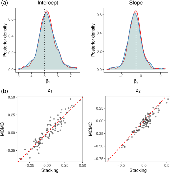
Figure 1. Simulated Poisson count data: (a) posterior distributions of the intercept as well as the slope obtained from stacking (blue) and MCMC (red) overlaid dotted vertical line showing their true values; (b) posterior medians of spatial-temporal random effects obtained by stacking and MCMC with the $y=x$ reference as a red dashed line.

Figure 1(a) shows the overlaid posterior densities of the fixed effects obtained from the stacked posterior (blue) and MCMC (red), revealing practically indistinguishable posterior distributions. Figure 1(b) displays high agreement between the posterior medians of the spatial-temporal random effects associated with the intercept and the slope, obtained by our proposed stacking algorithm and MCMC. We also notice that the posterior samples of the spatial-temporal process parameters do not necessarily concentrate around their true values hence, demonstrating their weak identifiability. In addition, we also observe similar patterns in the posterior distributions within the temporal ($\phi_{11}$ and $\phi_{12}$) and the spatial decay parameters ($\phi_{21}$ and $\phi_{22}$), which further motivates the assumptions of the reduced model (see, Figure A1 in Appendix C).

Treating the fully Bayesian model with priors on ${\theta_{\text{sp}}}$ which is fitted using MCMC, we find that the predictive performance of our proposed stacking algorithm gets closer to MCMC as sample size increases (see, Table 1). In Table 1, for Poisson count data, we see that, the difference in mean log-pointwise predictive density of 100 held-out samples between MCMC and our proposed stacking algorithm drops from 11.6% at sample size 100 to 10.5% at sample size 500. Furthermore, we find that the mean log-pointwise predictive density between MCMC on the “full” model (which has $2r$ process parameters) and MCMC on the reduced model drops from 10.1% at sample size 100 to 3.7% at sample size 500. We observe similar trend in case of the simulated binomial count data.

Model	Method	Sample size ($n$)
		$n=100$	$n=200$	$n=300$	$n=400$	$n=500$
Poisson	Stacking	-7.653	-7.594	-7.579	-7.538	-7.486
	rMCMC	-7.515	-7.398	-7.189	-7.066	-6.957
	MCMC	-6.758	-6.738	-6.736	-6.716	-6.696
Binomial	Stacking	-7.464	-7.449	-7.426	-7.411	-7.398
	rMCMC	-7.428	-7.389	-7.201	-7.182	-7.001
	MCMC	-6.978	-6.813	-6.747	-6.729	-6.711

Table 1. Predictive performance of stacking and MCMC. All values correspond to mean log-pointwise predictive density (MLPD) based on 5 replications. Stacking and rMCMC assumes the reduced model with shared process parameters while MCMC assumes separate process parameters.

5.3.2. Runtime comparison

Figure 2 reveals that predictive stacking is, on average, about 500 times faster than MCMC further corroborating the efficiency of predictive stacking as an alternative to MCMC. We have implemented our predictive stacking algorithm within the R statistical computing environment. We execute the programs for runtime comparisons on hardware equipped with an 1-Intel(R) Xeon(R) Gold 6140 CPU @ 2.30GHz processor with 36 cores and 1 thread per core, totalling 36 possible threads for parallel computing. The runtime for predictive stacking reported here are based on execution using 6 cores only. We compare the runtime of our proposed algorithm with the adaptive Metropolis-within-Gibbs algorithm that implements full Bayesian inference.

Figure 2. Comparison of runtimes of our proposed stacking algorithm (solid), MCMC (dashes) and MCMC on the reduced model (dot-dash). Stacking demonstrates significantly faster execution times across various sample sizes compared to the MCMC algorithms.

6. North American Breeding Bird Survey

Terrestrial birds were sampled annually from routes (approximately 40.23 km with point counts every 0.8 km) spread across the United States and Canada as part of the North American Breeding Bird Survey (Ziolkowski Jr. et al., 2022). We analyse the number of migrant birds observed at different locations across United States with the goal to predict their numbers at an arbitrary location. Our key inferential objective is to evaluate how the impact from nearby vehicles and external noise varies over space and time. For this analysis, we use 2,396 spatial coordinates over the years 2010 through 2019 at which the number of migrant birds were recorded. We aggregated the count data of different species within each spatial unit since very few locations recorded counts for more than one species. We consider two explanatory variables, “car” and “noise”. The variable ‘car’ represents tallies of vehicles passing survey points during each 3-minute count, and the variable ‘noise’ reports unrelated excessive noise at each point from sources other than passing vehicles (for example, from construction work). The presence of excessive noise is defined as noise lasting more than 45 seconds that significantly interferes with the observer’s ability to hear birds at the location during the sampling period. Both these variables are mapped to the same GPS coordinates in the form of latitude and longitude that reference the avian counts.

Statistical analysis of this survey has focused on different species-level analyses with random effects modelling variability within different levels of a factor. For example, Link and Sauer (1997) and Sauer and Link (2011) study route-level population trajectories of a species and observer effects using quasi-likelihood approaches and a Bayesian hierarchical log-linear model respectively. Sauer and Link (2011) elaborates on the practical difficulties arising from convergence issues compelling a limited number of MCMC iterations for moderately large datasets. Furthermore, their model featured random effects of much lower dimension than we have in our proposed model (7). In addition, none of the previous analyses uses spatial random effects in order to model spatial variability in their log-linear model whereas we utilise available geographic coordinates of the routes to build spatial-temporal processes to account for dependencies in the avian point count data within a rich modelling framework. This framework enables us to account for large scale variation in the mean using explanatory variables (for example the presence of excessive noise from vehicles) so the latent process evinces the residual spatial-temporal association in bird counts that can indicate lurking factors affecting the avian population.

We apply the spatial-temporal Poisson regression model in (7) to analyse the counts of migrant birds at the observed locations with ‘car’ and ‘noise’ as predictors having spatially-temporally varying regression coefficients with the correlation function as given in (8) and with the additional assumption of common process parameters $\phi_{1}$ and $\phi_{2}$ shared across all the spatial-temporal processes. We implemented our proposed stacking algorithm with $G_{\phi_{2}}=\{40,800,1000\}$ which considers the effective spatial range to be approximately 20%, 50% and 70% of the maximum inter-site distance, $G_{\phi_{1}}=\{0.5,1,2\}$, $G_{\sigma_{\xi}}=\{0.5,1\}$ and $G_{\alpha_{\epsilon}}=\{0.5,0.75\}$.

	Median	SD	2.5%	97.5%
(Intercept)	0.891	0.234	0.530	1.207
Car	0.007	0.054	-0.116	0.093
Noise	0.005	0.304	-0.395	0.508
Average Bird Count	15.789	20.677	13.529	31.753

Table 2. North American Breeding Bird Survey (2010-19): Posterior summary (95% credible intervals) of global regression coefficients and the average bird count over all spatial-temporal coordinates. SD denotes standard deviation; 2.5% and 97.5% represent quantiles.

Table 2 presents posterior summaries of global regression coefficients (the component that does not vary over space and time) for the intercept, ‘car’ and ‘noise’. We find the global intercept to be significantly larger than zero which contributes approximately 2.5 units to the count with 95% credible interval (1.7, 3.4) in the presence of no passing cars or excessive noise. Neither the number of cars nor levels of excessive noise seem to significantly impact the count in terms of global effects. The last row of Table 2 presents the estimated bird count averaged over all observed spatial-temporal coordinates in the data set. This estimate is obtained from the posterior predictive distribution of the average bird count and provides us with an estimate of the relative influence of the spatially-temporally varying component over the global effects. To be precise, we see that the spatially-temporally varying component of the regression increases the estimate of counts ($\approx$ 16) by a factor of 6 times over the 2.5 units contributed by the global effects. This estimate of the average bird count is consistent with what one would obtain from customary generalised linear models with fixed effects only, but we also offer the spatially and temporally varying impact of predictors that are not captured by the global regression.

Figures 3(a) and (b) reveal how the impact of the predictors ‘car’ and ‘noise’ vary over space and time. For example, in Fig. 3(a) we see significant positive impact (red) of ‘car’ in the Niland and Palo Verde regions of Imperial county, California, (southwest corner of the map) rather consistently between 2010 and 2012. These elevated spatial-temporal coefficients along with higher numbers of cars in these regions (not shown) produce higher than average estimates of bird counts there. We observe a similar pattern in parts of North Dakota and South Dakota between 2015 and 2019. Fig. 3(b) reveals a positive impact (red) of ‘noise’ in the spatial-temporal random effects in northern Minnesota from 2011 to 2015. While this area experiences persistently low levels of ‘noise’ (not shown) the high values of the coefficients produce higher than average estimates of bird counts. In summary, these spatially-temporally varying coefficients represent the local impact of predictors that adjusts the global effects from Table 2. Appendix D presents further details of this analysis.

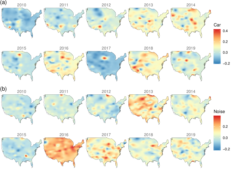
Figure 3. North American Breeding Bird Survey (2010-19): Interpolated surfaces of posterior median of spatial-temporal random effects in the slope of the variables (a) ‘car’ and, (b) ‘noise’ obtained by our proposed stacking algorithm.

Lastly, we note that while our proposed stacking algorithm delivered inference in 30 minutes using 6 cores, implementing the adaptive Metropolis-within-Gibbs algorithm anticipates at least 15,000 iterations for convergence with each iteration taking 1.3 minutes on average. Hence, our proposed stacking algorithm offers speed-ups of over 650 times over MCMC.

7. Discussion

We have devised and demonstrated Bayesian predictive stacking to be an effective tool for estimating spatially-temporally varying regression coefficients and yielding robust predictions for non-Gaussian spatial-temporal data. We develop and exploit analytically accessible distribution theory pertaining to Bayesian analysis of generalised linear mixed models that enables us to directly sample from the posterior distributions. The focus of this article is on effectively combining inference across different closed-form posterior distributions by circumventing inference on weakly identified parameters. Future developments and investigations will consider zero-inflated Bernoulli data for which the current approach will require a boundary adjustment parameter to ensure that the posterior distribution is well-defined. In this context, Bradley and Clinch (2024) explore flexible choices of $H$ to improve inference for zero-inflated Bernoulli data, although they lose the computational benefits arising from the structured $H$ in our spatially-temporally varying coefficients model. Exploring predictive stacking for alternate specifications of $H$ and, in particular, for zero-inflated binary data will comprise future research endeavours. Finally, our method can be adapted to variants of Gaussian process models that scale inference to massive datasets (Datta et al., 2016; Banerjee, 2017; Heaton et al., 2019) by circumventing the Cholesky decomposition of dense covariance matrices. Other directions can include building more general frameworks to accommodate irregular dispersion and analysis of zero-inflated count data.

Data and code availability

Codes and data required to reproduce the results and findings in this article are openly available on GitHub (https://github.com/SPan-18/spatialGLM_stacking). The North American Breeding Bird survey database is openly available at https://doi.org/10.5066/P97WAZE5.

Conflicts of interest

All authors declare that they have no conflicts of interest.

Appendix to “Bayesian inference for spatial-temporal non-Gaussian data
using predictive stacking”

Appendix A Distribution theory

We outline relevant distribution theory for deriving the posterior distribution of different model parameters in the Bayesian hierarchical model (7) in the main article. Our contribution lies in proving two important results, Proposition A1 and Lemma A1, that justifies constructing the improper prior for the parameter $q$, also referred to as the discrepancy parameter (Bradley et al., 2020) and has not been addressed hitherto (Bradley and Clinch, 2024, Theorem 3.1). We assume familiarity with the notations introduced in Section 3 of the main article.

Proposition A1.

If $H=[(I_{n}:X_{n\times p}:\tilde{X}_{n\times nr})^{{\top}}:I_{n+p+nr}]^{{\top}}$ and $Q=[Q_{1}^{{\top}}:Q_{2}^{{\top}}]^{{\top}}$, where $Q$ is $(2n+p+nr)\times n$ with $Q_{1}$ being $n\times n$ and $Q_{2}$ being $(n+p+nr)\times n$, such that the $n$ columns of $Q$ are the unit norm orthogonal eigenvectors of the orthogonal projector, $P_{H}$, on the column space of $H$, then $\mathrm{rank}(Q_{1})=n$.

Proof.

From our definitions, we note that $QQ^{{\top}}=I_{2n+p+nr}-P_{H}$, $P_{H}=H(H^{{\top}}H)^{-1}H^{{\top}}$, $Q^{{\top}}H=0$ and $\mathrm{rank}(Q)=n$. Define $H_{1}=[I_{n}:X:\tilde{X}]$. It follows from $Q^{{\top}}H=0$ that, $Q_{1}^{{\top}}H_{1}+Q_{2}^{{\top}}=0$ and subsequently, $Q_{2}=-H_{1}^{{\top}}Q_{1}$, implying that $\mathscr{R}(Q_{2})\subseteq\mathscr{R}(Q_{1})$ where $\mathscr{R}$ denotes row space of a matrix. Hence the rank of $Q$ must equal $\dim(\mathscr{R}(Q_{1}))$, the number of independent rows of $Q_{1}$. As $\mathrm{rank}(Q)=n$, we have $\mathrm{rank}(Q_{1})=\dim(\mathscr{R}(Q_{1}))=n$. ∎

Lemma A1.

In the hierarchical model (7), assumption of a vague prior on the parameter $\mu$ leads to the improper prior on the parameter $q$, given by $p(q)\propto 1$.

Proof.

Recall that $q=-Q^{{\top}}\tilde{\mu}$ where $\tilde{\mu}=(\mu^{{\top}},\mu_{\gamma}^{{\top}})^{{\top}}$ with $\mu_{\gamma}=(\mu_{\xi}^{{\top}},\mu_{\beta}^{{\top}},\mu_{z}^{{\top}})^{{\top}}$ and $Q$ is the $(2n+p+nr)\times n$ matrix defined in Proposition A1. Partition $Q=[Q_{1}^{\top}:Q_{2}^{\top}]^{\top}$ where $Q_{1}$ is $n\times n$ and $Q_{2}$ is $(n+p+nr)\times n$ to get $q=-Q_{1}^{\top}\mu-Q_{2}^{\top}\mu_{\gamma}$. Consider the sequence of priors on the discrepancy parameter as $p_{1,k}(\mu)=\mathcal{N}(\mu\mid 0_{n},\tau_{k}I_{n})$ for a real sequence $\{\tau_{k}\}_{k\in\mathbb{N}}$ with $\tau_{k}>0,\forall k\in\mathbb{N}$ such that $\lim_{k}\tau_{k}=+\infty$. By Proposition A1, for any $k$, the prior on $q$ induced by $p_{1,k}$ has the density $p_{2,k}(q)=\mathcal{N}(q\mid-Q_{2}^{\top}\mu_{\gamma},\tau_{k}Q_{1}^{\top}Q_{1})$. Hence, the improper density $p_{2}(q)\propto 1$ arises from $\lim_{k}p_{2,k}(q)=p_{2}(q)$ for any $q\in\mathbb{R}^{n}$. ∎

Next, we derive the posterior distribution in (9) corresponding to the hierarchical model (7) in the main article. The following result adapts the spatial intercept model of Theorem 3.1 in Bradley and Clinch (2024) to our spatially-temporally varying coefficient model. This extension is not entirely straightforward because of the introduction of possibly different explanatory variables in the fixed regression ($X$) and the spatially-temporally varying component ($\tilde{X}$) in our model.

Theorem A1.

The hierarchical model (7), with $p(q)\propto 1$ leads to

$$p\left((\gamma^{\top},q^{\top})^{\top}\mid y,\theta\right)\propto\mathrm{GCM}\left((\gamma^{\top},q^{\top})^{\top}\mid 0_{2n+p+nr},V^{*}(\theta),\alpha^{*},\kappa^{*};\psi^{*}\right)\;,$$

where $V^{*}(\theta)^{-1}=L(\theta)^{-1}[H:Q]$, $(3n+p)\times(3n+p)$ block-diagonal matrix $L(\theta)=\mathrm{blkdiag}(I_{n},\sigma_{\xi}I_{n},\allowbreak\sigma_{\beta}L_{\beta},L_{z}(\theta))$ with $\sigma_{z_{j}}L_{z_{j}}({\theta_{\text{sp}}})$ as the $j$th block of $nr\times nr$ block-diagonal matrix $L_{z}(\theta)$. The shape and scale parameters are $\alpha^{*}=((y+\alpha_{\epsilon}1_{n})^{\top},0_{n}^{\top},\alpha_{\beta}^{\top},\alpha_{z}^{\top})^{\top}$ and $\kappa^{*}=((b+\kappa_{\epsilon})1_{n}^{\top},(1/2)1_{n}^{\top},\kappa_{\beta}^{\top},\kappa_{z}^{\top})^{\top}$. The unit log partition function $\psi^{*}$ is $\psi^{*}(h)=(\psi_{y}(h_{1})^{{\top}},\psi_{1}(h_{2})^{{\top}},\psi_{\beta}(h_{3})^{{\top}},\psi_{z}(h_{4})^{{\top}})$ for some $h=(h_{1}^{{\top}},h_{2}^{{\top}},h_{3}^{{\top}},h_{4}^{{\top}})^{{\top}}$ with $h_{1},h_{2}\in\mathbb{R}^{n}$, $h_{3}\in\mathbb{R}^{p}$, $h_{4}\in\mathbb{R}^{nr}$, and, $\psi_{z}(h_{4})=(\psi_{z_{1}}(h_{41}),\ldots,\psi_{z_{r}}(h_{4r}))$ for $h_{4j}\in\mathbb{R}^{n}$, where all of the log partition functions operate element-wise on the arguments.

Proof.

Define the $(n+p+nr)\times 1$ random vector $\gamma=(\xi^{\top},\beta^{\top},z^{\top})^{\top}$. Then the likelihood is

$$\begin{split}p(y\mid\gamma,\mu)&=\exp\left\{y^{\top}(X\beta+\tilde{X}z+\xi-\mu)-b1_{n}^{T}\psi_{y}(X\beta+\tilde{X}z+\xi-\mu)\right\}\\ &=\exp\left\{y^{\top}\left(\begin{bmatrix}I_{n}&X&\tilde{X}\end{bmatrix}\gamma-\mu\right)-b1_{n}^{T}\psi_{y}\left(\begin{bmatrix}I_{n}&X&\tilde{X}\end{bmatrix}\gamma-\mu\right)\right\}.\end{split}$$ (A1)

According to Section 2.2, the densities of $\mathrm{CM}$ priors for $\beta\mid\theta$ and $z\mid\theta$ are

$$\begin{split}p(\beta\mid\theta)&\propto\exp\left\{\alpha_{\beta}^{\top}L_{\beta}(\theta)^{-1}(\beta-\mu_{\beta})-\kappa_{\beta}^{\top}\psi_{\beta}(L_{\beta}(\theta)^{-1}(\beta-\mu_{\beta}))\right\}\;,\\ p(z\mid\theta)&\propto\exp\left\{\alpha_{z}^{\top}L_{z}(\theta)^{-1}(z-\mu_{z})-\kappa_{z}^{\top}\psi_{z}(L_{z}(\theta)^{-1}(z-\mu_{z}))\right\}\;,\end{split}$$ (A2)

where $nr\times nr$ matrix $L_{z}(\theta)=\oplus_{j=1}^{r}\sigma_{z_{j}}L_{z_{j}}({\theta_{\text{sp}}}_{j})$. And the conditional prior $p(\xi\mid\beta,z,\theta)$ is

$$\begin{split}p(\xi\mid\beta,z,\mu,\theta)&\propto\exp\left\{\alpha_{\xi}^{\top}\left(\begin{bmatrix}I_{n}\\ L_{\xi}(\theta)^{-1}\end{bmatrix}\xi-\begin{bmatrix}\mu-X\beta-\tilde{X}z\\ L_{\xi}(\theta)^{-1}\mu_{\xi}\end{bmatrix}\right)\right.\\ &\quad\left.-\kappa_{\xi}^{\top}\psi_{\xi}\left(\begin{bmatrix}I_{n}\\ L_{\xi}(\theta)^{-1}\end{bmatrix}\xi-\begin{bmatrix}\mu-X\beta-\tilde{X}z\\ L_{\xi}(\theta)^{-1}\mu_{\xi}\end{bmatrix}\right)\right\}\\ &=\exp\left\{\alpha_{\xi}^{\top}\left(\begin{bmatrix}I_{n}&X&\tilde{X}\\ L_{\xi}(\theta)^{-1}&0&0\end{bmatrix}\gamma-\begin{bmatrix}\mu\\ L_{\xi}(\theta)^{-1}\mu_{\xi}\end{bmatrix}\right)\right.\\ &\quad\left.-\kappa_{\xi}^{\top}\psi_{\xi}\left(\begin{bmatrix}I_{n}&X&\tilde{X}\\ L_{\xi}(\theta)^{-1}&0&0\end{bmatrix}\gamma-\begin{bmatrix}\mu\\ L_{\xi}(\theta)^{-1}\mu_{\xi}\end{bmatrix}\right)\right\}\;,\end{split}$$ (A3)

where the last step follows from equality

$$\begin{bmatrix}I_{n}\\ L_{\xi}(\theta)^{-1}\end{bmatrix}\xi-\begin{bmatrix}\mu-X\beta-\tilde{X}z\\ L_{\xi}(\theta)^{-1}\mu_{\xi}\end{bmatrix}=\begin{bmatrix}I_{n}&X&\tilde{X}\\ L_{\xi}(\theta)^{-1}&0&0\end{bmatrix}\gamma-\begin{bmatrix}\mu\\ L_{\xi}(\theta)^{-1}\mu_{\xi}\end{bmatrix}.$$

Hence, combining (A2) and (A3) yields the joint prior density $p(\gamma\mid\mu,\theta)$ as

$$\begin{split}p\left(\gamma\mid\mu,\theta\right)&\propto\exp\left\{(\alpha_{\xi}^{\top},\alpha_{\beta}^{\top},\alpha_{z}^{\top})\left(\begin{bmatrix}I_{n}&X&\tilde{X}\\ L_{\xi}(\theta)^{-1}&0&0\\ 0&L_{\beta}(\theta)^{-1}&0\\ 0&0&L_{z}(\theta)^{-1}\end{bmatrix}\begin{bmatrix}\xi\\ \beta\\ z\end{bmatrix}-\begin{bmatrix}\mu\\ L_{\xi}(\theta)^{-1}\mu_{\xi}\\ L_{\beta}(\theta)^{-1}\mu_{\beta}\\ L_{z}(\theta)^{-1}\mu_{z}\end{bmatrix}\right)\right.\\ &\quad\left.-(\kappa_{\xi}^{\top},\kappa_{\beta}^{\top},\kappa_{z}^{\top})\psi^{*}\left(\begin{bmatrix}I_{n}&X&\tilde{X}\\ L_{\xi}(\theta)^{-1}&0&0\\ 0&L_{\beta}(\theta)^{-1}&0\\ 0&0&L_{z}(\theta)^{-1}\end{bmatrix}\begin{bmatrix}\xi\\ \beta\\ z\end{bmatrix}-\begin{bmatrix}\mu\\ L_{\xi}(\theta)^{-1}\mu_{\xi}\\ L_{\beta}(\theta)^{-1}\mu_{\beta}\\ L_{z}(\theta)^{-1}\mu_{z}\end{bmatrix}\right)\right\}\;,\end{split}$$ (A4)

where $\psi^{*}(h)=(\psi_{y}(h_{1})^{{\top}},\psi_{1}(h_{2})^{{\top}},\psi_{\beta}(h_{3})^{{\top}},\psi_{z}(h_{4})^{{\top}})$ for some $h=(h_{1}^{{\top}},h_{2}^{{\top}},h_{3}^{{\top}},h_{4}^{{\top}})^{{\top}}$ with $h_{1},h_{2}\in\mathbb{R}^{n}$, $h_{3}\in\mathbb{R}^{p}$, $h_{4}\in\mathbb{R}^{nr}$, and, $\psi_{z}(h_{4})=(\psi_{z_{1}}(h_{41}),\ldots,\psi_{z_{r}}(h_{4r}))$ for $h_{4j}\in\mathbb{R}^{n}$, where all the log partition functions operates element-wise on the arguments. Hence, assuming $p(q)\propto 1$, we obtain

$$\begin{split}p\left((\gamma^{\top},q^{\top})^{\top}\mid y,\theta\right)&\propto\exp\left\{(y^{\top}+\alpha_{\epsilon}1_{n}^{\top},0_{n}^{\top},\alpha_{\beta}^{\top},\alpha_{z}^{\top})L(\theta)^{-1}(H\gamma-\tilde{\mu})\right.\\ &\qquad\left.-((b+\kappa_{\epsilon})1_{n}^{\top},\frac{1}{2}1_{n}^{\top},\kappa_{\beta}^{\top},\kappa_{z}^{\top})\psi^{*}L(\theta)^{-1}(H\gamma-\tilde{\mu})\right\}\\ &=\exp\left\{\alpha^{*{\top}}L(\theta)^{-1}(H\gamma-\tilde{\mu})-\kappa^{*{\top}}\psi^{*}(L(\theta)^{-1}(H\gamma-\tilde{\mu}))\right\}\end{split}$$ (A5)

by combining (A1) and (A4). Now, reparameterise by $q=-Q^{\top}\tilde{\mu}$, which, by definition of $Q$ (see Section 3.2), is equivalent to $\tilde{\mu}=-Qq$, and, thus from (A5), we obtain

$$\begin{split}p\left((\gamma^{\top},q^{\top})^{\top}\mid y,\theta\right)&=\exp\left\{\alpha^{*{\top}}L(\theta)^{-1}[H:Q]\begin{bmatrix}\gamma\\ q\end{bmatrix}-\kappa^{*{\top}}\psi^{*}\left(L(\theta)^{-1}[H:Q]\begin{bmatrix}\gamma\\ q\end{bmatrix}\right)\right\}\\ &\propto\mathrm{GCM}\left((\gamma^{\top},q^{\top})^{\top}\mid 0_{3n+p},V^{*}(\theta),\alpha^{*},\kappa^{*};\psi^{*}\right).\end{split}$$ (A6)

∎

Appendix B Computational details

This section evolves as follows. First, we present Theorem A2 that provides a computationally efficient way to evaluate the projection expression in (11) in the main article and subsequently provide a memory-efficient algorithm implementing Theorem A2. Next, we outline the algorithm for fast Cholesky factor updates required for the cross-validation step, as detailed in Section 4.4 of the main article. Lastly, we summarise our proposed stacking algorithm in Algorithm S3.

Once the Cholesky factors are computed, we are able to obtain the samples, $\tilde{v}_{z}$, from the marginal prior of $z$. Given $\tilde{v}$, following Section 4.2, it is clear that naive evaluation of $\gamma^{(r)}=(H^{\top}H)^{-1}H^{\top}\tilde{v}$ requires expensive matrix operations on an $(n+p+nr)\times(n+p+nr)$ matrix $H^{\top}H$. Theorem A2 derives a computationally efficient algorithm to evaluate this projection.

Theorem A2.

Given $\tilde{v}$, the projection expression in (11) can be computed in $O(nr^{3}+p^{3})$ flops and requires a storage of $O(np+nr+nr^{2}+p^{2})$.

Proof.

Note that $H=[(I_{n}:X:\tilde{X})^{\top}:I_{n+p+nr}]^{\top}$ is a $(2n+p+nr)\times(n+p+nr)$ matrix where $\tilde{X}=[\mathrm{diag}(\tilde{x}_{1}):\cdots:\mathrm{diag}(\tilde{x}_{r})]$ is $n\times nr$ with $\mathrm{diag}(\tilde{x}_{j})$ being an $n\times n$ diagonal matrix whose $i$th diagonal element is $\tilde{x}_{j}(\ell_{i})$. Without loss of generality, we consider a permutation of the columns of $\tilde{X}$ and a subsequent suitable permutation on $z=(z_{1}^{\top},\ldots,z_{r}^{\top})$ such that the new $\tilde{X}=\oplus_{i=1}^{n}\tilde{x}_{i}^{\top}$ and $z=(z_{(1)}^{\top},\ldots,z_{(n)}^{\top})^{\top}$ where $z_{(i)}=(z_{1}(\ell_{i}),\ldots,z_{r}(\ell_{i}))^{\top}$. Note that we can always rearrange the obtained vector back to the original ordering by applying the inverse of the permutation. The idea of the proof follows from inversion of a partitioned matrix. Write

$$H^{\top}H=\begin{bmatrix}2I_{n}&X&\tilde{X}\\ X^{\top}&X^{\top}X+I_{p}&X^{\top}\tilde{X}\\ \tilde{X}^{\top}&\tilde{X}^{\top}X&\tilde{X}^{\top}\tilde{X}+I_{nr}\end{bmatrix}=\begin{bmatrix}A&B^{\top}\\ B&D\end{bmatrix}\;,$$ (A7)

where $B=[\tilde{X}^{\top}:\tilde{X}^{\top}X]$ and $D=\tilde{X}^{\top}\tilde{X}+I_{nr}$. Note that $(H^{\top}H)^{-1}H^{\top}\tilde{v}$ can be simplified as

$$(H^{\top}H)^{-1}H^{\top}\tilde{v}=\begin{bmatrix}S_{A}^{-1}(v_{1}-B^{\top}D^{-1}v_{2})\\ -D^{-1}BS_{A}^{-1}(v_{1}-B^{\top}D^{-1}v_{2})+D^{-1}v_{2}\end{bmatrix}\;,$$ (A8)

where $v_{1}=((\tilde{v}_{\eta}+\tilde{v}_{\xi})^{\top},(X^{\top}\tilde{v}_{\eta}+\tilde{v}_{\beta})^{\top})^{\top}$, $v_{2}=(\tilde{X}^{\top}\tilde{v}_{\eta}+\tilde{v}_{z})^{\top}$ and $S_{A}$ denotes the Schur complement of $A$ in (A7). Define $v_{3}=v_{1}-B^{\top}D^{-1}v_{2}$ and rewrite it as $v_{1}-[(\tilde{X}v_{4})^{\top},(X^{\top}\tilde{X}v_{4})^{\top}]^{\top}$ where $v_{4}=(\tilde{X}^{\top}\tilde{X}+I_{nr})^{-1}v_{2}$. Note that $v_{4}$ can be evaluated efficiently since $(\tilde{X}^{\top}\tilde{X}+I_{nr})^{-1}=\oplus_{i=1}^{n}(\tilde{x}_{i}\tilde{x}_{i}^{\top}+I_{r})^{-1}$ is block diagonal. This involves $n$ inversions of $r\times r$ positive definite matrices and hence evaluation of $v_{4}$ involves $O(nr^{3})$ operations. Next, we move on to inversion of the Schur complement $S_{A}=A-B^{\top}D^{-1}B$. Note that $B^{\top}D^{-1}B=[I_{n}:X]^{\top}\tilde{X}(\tilde{X}^{\top}\tilde{X}+I_{nr})^{-1}\tilde{X}^{\top}[I_{n}:X]$. We use $(\tilde{X}^{\top}\tilde{X}+I_{nr})^{-1}\tilde{X}^{\top}=\tilde{X}^{\top}(\tilde{X}\tilde{X}^{\top}+I_{n})^{-1}$ which follows from the equality $\tilde{X}^{\top}(\tilde{X}\tilde{X}^{\top}+I_{n})=(\tilde{X}^{\top}\tilde{X}+I_{nr})\tilde{X}^{\top}$. Hence we have $\tilde{X}(\tilde{X}^{\top}\tilde{X}+I_{nr})^{-1}\tilde{X}^{\top}=\tilde{X}\tilde{X}^{\top}(\tilde{X}\tilde{X}^{\top}+I_{n})^{-1}=\mathrm{diag}(\lVert\tilde{x}_{i}\rVert^{2}/(1+\lVert\tilde{x}_{i}\rVert^{2}),i=1,\ldots,n)=\tilde{P}$ (say). Then, writing $v_{3}=(v_{51}^{\top},v_{52}^{\top})^{\top}$,

$$S_{A}=\begin{bmatrix}A_{*}&B_{*}^{\top}\\ B_{*}&D_{*}\end{bmatrix},\quad S_{A}^{-1}v_{3}=\begin{bmatrix}A_{*}^{-1}v_{51}+A_{*}^{-1}B_{*}^{\top}S_{D_{*}}^{-1}(B_{*}A_{*}^{-1}v_{51}-v_{52})\\ -S_{D_{*}}^{-1}(B_{*}A_{*}^{-1}v_{51}-v_{52})\end{bmatrix}\;,$$ (A9)

where $v_{51}$ is $n\times 1$, $v_{52}$ is $p\times 1$ and, $A_{*}=2I_{n}-\tilde{P}$, $B_{*}=X^{\top}(I_{n}-\tilde{P})$, $D_{*}=X^{\top}(I_{n}-\tilde{P})X+I_{p}$. Note that $A_{*}^{-1}=(2I_{n}-\tilde{P})^{-1}$ is again a diagonal matrix with diagonal elements $(1+\lVert\tilde{x}_{i}\rVert^{2})/(2+\lVert\tilde{x}_{i}\rVert^{2})$ for $i=1,\ldots,n$. Hence, we evaluate $v_{6}=B_{*}A_{*}^{-1}v_{51}-v_{52}=X^{\top}\mathrm{diag}(1/(2+\lVert\tilde{x}_{i}\rVert^{2}))v_{51}-v_{52}$. Finally, we find the inverse of $S_{D_{*}}$, the $p\times p$ Schur complement of $D_{*}$, by simplifying as

$$\begin{split}S_{D_{*}}&=D_{*}-B_{*}A_{*}^{-1}B_{*}^{\top}\\ &=X^{\top}(I-\tilde{P})X+I_{p}-X^{\top}(I_{n}-\tilde{P})(2I_{n}-\tilde{P})^{-1}(I_{n}-\tilde{P})X\\ &=I_{p}+X^{\top}\left[\mathrm{diag}\left(\frac{1}{1+\lVert\tilde{x}_{i}\rVert^{2}}\right)-\mathrm{diag}\left(\frac{1}{1+\lVert\tilde{x}_{i}\rVert^{2}}\right)\mathrm{diag}\left(\frac{1+\lVert\tilde{x}_{i}\rVert^{2}}{2+\lVert\tilde{x}_{i}\rVert^{2}}\right)\mathrm{diag}\left(\frac{1}{1+\lVert\tilde{x}_{i}\rVert^{2}}\right)\right]X\\ &=I_{p}+X^{\top}\mathrm{diag}\left(\frac{1}{2+\lVert\tilde{x}_{i}\rVert^{2}}\right)X.\end{split}$$ (A10)

Inverting $S_{D_{*}}$ takes $O(p^{3})$ operations thus completing the evaluation of $S_{A}^{-1}v_{3}$. We subsequently find $D^{-1}BS_{A}^{-1}v_{3}$ using the already computed block inverses of the matrix $D$. ∎

Next, Algorithm S1 provides a memory-efficient step-by-step implementation of Theorem A2. It proceeds by considering the $n\times nr$ predictor matrix $\tilde{X}$ with permuted columns as described in Theorem A2. Subsequently $\tilde{v}_{z}$ is also permuted adapting to the new $\tilde{X}$. This requires memory allocations for one $nr\times 1$ vector $v_{1}$, two $n\times 1$ vectors $v_{2}$ and $v_{4}$, one $p\times 1$ vector $v_{3}$, an $n$-dimensional list $\{D_{i}:i=1,\ldots,n\}$ with each item storing one $r\times r$ matrix and one $p\times p$ matrix $D_{*}$, amounting to allocated storage of $O(n+p+nr+p^{2}+nr^{2})$.

Algorithm S1 Computationally efficient algorithm for projection (see, Theorem A2)

1:Input: $X$, $\tilde{X}$, $\tilde{v}_{\eta}$, $\tilde{v}_{\xi}$, $\tilde{v}_{\beta}$, $\tilde{v}_{z}$

2:Output: Posterior samples of $\gamma=(\xi^{\top},\beta^{\top},z^{\top})^{\top}$

3:Storage: Pre-allocate $v_{1}$, $v_{2}$, $v_{3}$, $v_{4}$, $\{D_{i}:i=1,\ldots,n\}$, $D_{*}$

4:function projection($X$, $\tilde{X}$, $\tilde{v}_{\eta}$, $\tilde{v}_{\xi}$, $\tilde{v}_{\beta}$, $\tilde{v}_{z}$)

5:     $v_{1}\leftarrow\tilde{X}^{\top}\tilde{v}_{\eta}+\tilde{v}_{z}$

6:     for $i=1$ to $i=n$ do

7:         $D_{i}\leftarrow\texttt{chol}\left(\tilde{x}_{i}\tilde{x}_{i}^{\top}+I_{r}\right)$

8:         $v_{1,i}\leftarrow\texttt{trsolve}(D_{i},v_{1,i})$      

9:     $v_{2}\leftarrow\tilde{v}_{\eta}-\tilde{X}v_{1}$

10:     $v_{3}\leftarrow X^{\top}v_{2}+\tilde{v}_{\beta}$

11:     $v_{2}\leftarrow v_{2}+\tilde{v}_{\xi}$

12:     for $i=1$ to $i=n$ do $v_{4,i}\leftarrow v_{2,i}/(2+\lVert\tilde{x}_{i}\rVert^{2})$      

13:     $v_{3}\leftarrow X^{\top}v_{4}-v_{3}$

14:     $D_{*}\leftarrow\texttt{chol}\left(I_{p}+X^{\top}\mathrm{diag}\left(\frac{1}{2+\lVert\tilde{x}_{i}\rVert^{2}}\right)_{i=1}^{n}X\right)$

15:     $v_{3}\leftarrow\texttt{trsolve}(D_{*},v_{3})$

16:     $v_{4}\leftarrow Xv_{3}$

17:     $v_{2}\leftarrow\mathrm{diag}\left(\frac{1+\lVert\tilde{x}_{i}\rVert^{2}}{2+\lVert\tilde{x}_{i}\rVert^{2}}\right)_{i=1}^{n}v_{2}+\mathrm{diag}\left(\frac{1}{2+\lVert\tilde{x}_{i}\rVert^{2}}\right)_{i=1}^{n}v_{4}$

18:     $v_{4}\leftarrow v_{2}-v_{4}$

19:     for $i=1$ to $i=n$ do

20:         $v_{1,i}\leftarrow\texttt{trsolve}(D_{i},v_{4,i}\tilde{x}_{i})$      

21:     return $(v_{2}^{\top},-v_{3}^{\top},-v_{1}^{\top})^{\top}$

Throughout Algorithm S1, while $v_{2,i}$ and $v_{4,i}$ correspond to the $i$th element of the $n\times 1$ vectors $v_{2}$ and $v_{4}$, respectively, $v_{1,i}$ denotes the $i$th $r\times 1$ block of the $nr\times 1$ vector $v_{1}$ corresponding to the indices running from $(i-1)r+1$ to $ir$ for each $i=1,\ldots,n$. The functions chol and trsolve compute the standard Cholesky decomposition and the solution of a triangular linear system, respectively, and are readily available in numerical linear algebra libraries. Algorithm S1 has been designed to avoid expensive linear algebra, consisting of $n$ Cholesky decompositions of $r\times r$ matrices, one Cholesky decomposition of a $p\times p$ matrix, $2n$ triangular solvers each of order $O(r)$, and one additional $O(p)$ triangular solve.

Next, we supply a block Givens rotation algorithm (Golub and Van Loan, 2013, Section 5.1.8) for faster model evaluation during cross-validation. Our algorithm can be regarded as a block-level variant of Kim et al. (2002). Following the setup preceding Algorithm S3, suppose the $k$th block $\chi_{[k]}$ for each $k$ contains adjacent indices of the data $\chi$. Moreover, suppose evaluating a model needs Cholesky decomposition of a $n\times n$ positive-definite matrix $R$, where $n$ is the number of observations in $\chi$. In the context of (7), $R$ corresponds to the correlation matrix of a spatial-temporal process. Suppose we have evaluated the model on the full data, and we have stored $L$, the upper triangular Cholesky factor of $R$. The consecutive indices of the partitioned data creates $K^{2}$ submatrices partitioning $R$ and its upper triangular Cholesky factor $L$ as,

$$R=\begin{bmatrix}R_{11}&R_{21}^{\top}&\cdots&R_{K1}^{\top}\\ R_{21}&R_{22}&\cdots&R_{K2}^{\top}\\ \vdots&\vdots&\ddots&\vdots\\ R_{K1}&R_{K2}&\cdots&R_{KK}\end{bmatrix},\quad L=\begin{bmatrix}L_{11}&L_{12}&\cdots&L_{1K}\\ 0&L_{22}&\cdots&L_{2K}\\ \vdots&\vdots&\ddots&\vdots\\ 0&0&\cdots&L_{KK}\end{bmatrix}.$$

For each $k$ such that $1<k<K$, consider the following representation of the matrices $R$, $L$, $R_{-k}$, the matrix corresponding to $\chi_{[-k]}$ and its upper triangular Cholesky factor $L_{-k}$.

$$R=\begin{bmatrix}R_{11}^{k}&R_{21}^{k{\top}}&R_{31}^{k{\top}}\\ R_{21}^{k}&R_{22}^{k}&R_{32}^{k{\top}}\\ R_{31}^{k}&R_{32}^{k}&R_{33}^{k}\end{bmatrix},\quad L=\begin{bmatrix}L_{11}^{k}&L_{12}^{k}&L_{13}^{k}\\ 0&L_{22}^{k}&L_{23}^{k}\\ 0&0&L_{33}^{k}\end{bmatrix},\quad R_{-k}=\begin{bmatrix}R_{11}^{k}&R_{31}^{k{\top}}\\ R_{31}^{k}&R_{33}^{k}\end{bmatrix},\quad L_{-k}=\begin{bmatrix}C_{11}^{k}&C_{13}^{k}\\ 0&C_{33}^{k}\end{bmatrix}\;,$$

where $R_{22}^{k}=R_{kk}$. Then, Algorithm S2 finds $L_{-k}$ for each $k=1,\ldots,K$. In Algorithm S2, note that, no computation is needed to find $L_{-K}$ and $C_{11}^{k}$, $C_{13}^{k}$ for $1<k<K$.

Algorithm S2 Fast Cholesky updates of row-deletion using block Givens rotation.

1:Input: $R$, $L$, $k$; full matrix, its upper-triangular Cholesky factor, block to be deleted

2:Output: $L_{-k}$, the Cholesky factor of $R_{-k}$, the matrix with $k$th block deleted

3:function choleskyCV($R$, $L$, k)

4:     if $k=1$ then

5:         $L_{-k}\leftarrow\texttt{chol}(R_{-k})$

6:     else

7:         if $1<k<K$ then

8:              $C_{11}^{k}\leftarrow L_{11}^{k}$ (pre-computed)

9:              $C_{13}^{k}\leftarrow L_{13}^{k}$ (pre-computed)

10:              $C_{33}^{k}\leftarrow\texttt{chol}(L_{33}^{k{\top}}L_{33}^{k}+L_{23}^{k{\top}}L_{23}^{k})$

11:         else

12:              $L_{-k}=$ upper left $(K-1)\times(K-1)$ submatrices of $L$ (pre-computed)               

13:     return $L_{-k}$

It is worth remarking that the “naive approach” for obtaining $L_{-k}$ involves Cholesky decomposition of $R_{k}$ for each $k$, and, hence, requiring $K^{-2}(K-1)^{3}n^{3}/3$ floating point operations (flops). On the other hand, the time complexity of Algorithm S2 is in the order of

$$\sum_{k=1}^{K}\left(1-\frac{k}{K}\right)^{3}\frac{n^{3}}{3}=\frac{n^{3}}{3K^{3}}\sum_{k=1}^{K-1}i^{3}=\frac{n^{3}}{3K^{3}}\frac{K^{2}(K-1)^{2}}{4}=\frac{(K-1)^{2}}{4K}\frac{n^{3}}{3}\;,$$

where the penultimate step follows from the sum of cubes of natural numbers. Hence, we show that Algorithm S2 is theoretically $4(K-1)/K$ times faster than the naive approach. If $K=10$ (Vehtari and Lampinen, 2002), then Algorithm S2 theoretically offers approximately 72% efficiency in time complexity over the naive approach. However, it must be noted that modern linear algebra libraries are highly vectorised and are often multithreaded. Hence, it is difficult to accurately translate these purely theoretical flop counts to actual wall clock time. Nevertheless, Algorithm S2 is more efficient than the naive approach.

Lastly, we detail the algorithm for implementing our proposed stacking framework utilising the aforementioned algorithms. Algorithm S3 outlines the steps required for estimating the spatially-temporally varying coefficients model (7) in the main article. The inputs $X$ and $\tilde{X}$ in Algorithm S3 correspond to the design matrices appearing in (7), $\mathcal{L}$ denotes spatial-temporal locations, $N$ denotes number of posterior samples to be drawn, $B$ denotes the number of samples to be drawn for evaluating the leave-one-out predictive densities as described in (15), $\mathcal{M}=\{M_{1},\ldots,M_{L}\}$ denotes the collection of $L$ candidate models and $K$ denotes the number of folds for cross-validation required for fast evaluation of leave-one-out predictive densities. Following a random permutation of the entire dataset, we construct a partition using consecutive indices of the permuted data. This step significantly accelerates evaluation of Cholesky factors using block Givens rotation (Golub and Van Loan, 2013) required during the cross-validation step detailed in Algorithm S2. After partitioning the data, which is denoted by $\chi=(y,X,\tilde{X},\mathcal{L})$ into $K$ blocks, each block is denoted by $\chi_{[k]}$ and the data with the $k$th block deleted is denoted by $\chi_{[-k]}$ for $k=1,\ldots,K$. Algorithm S3 is written in a richer and more general context and can be easily adapted to spatial, spatial-temporal, spatially and spatially-temporally varying coefficients models.

Algorithm S3 Predictive stacking algorithm for spatially-temporally varying coefficients GLM

1:Input: $y$, $X$, $\tilde{X}$, $\mathcal{L}$, $N$, $B$, $\mathcal{M}$, $K$

2:Output: Posterior samples for each model in $\mathcal{M}$, optimal stacking weights $\hat{w}$

3:function stvcGLM_stacking($y,X,\tilde{X},\mathcal{L},N,B,\mathcal{M},K$)

4:     Partition the data $\chi$ into $K$ blocks $\chi_{[1]},\ldots,\chi_{[K]}$, each containing consecutive indices

5:     for $l=1$ to $l=L$ do

6:         Fit model $M_{l}$ on $\chi$ and obtain posterior samples $\{\beta_{l}^{m},z_{l}^{m}\}_{m=1}^{N}$ using (11)

7:         for $k=1$ to $k=K$ do

8:              Fit model $M_{l}$ on $\chi_{[-k]}$ and obtain posterior samples $\{\beta_{k,l}^{s},z_{k,l}^{s}\}_{s=1}^{S}$ using (11)

9:              for $s=1$ to $s=S$ do

10:                  Use (13) to predict the spatial-temporal process $\tilde{z}_{k,l}^{s}$ at $\mathcal{L}_{[k]}$ from $z_{k,l}^{s}$               

11:              Use (15) to find $p(y(\ell_{i})\mid y_{-i},M_{l}),\ell_{i}\in\mathcal{L}_{[k]}$               

12:     Optimise (14) to obtain optimal stacking weights $\hat{w}$

13:     return Optimal model weights $\hat{w}$, Posterior samples $\{\beta_{l}^{m},z_{l}^{m}\}_{m=1}^{N}$ for $l=1,\ldots,L$

Appendix C Additional details on simulation experiments

We present some additional results from the simulation experiments carried out in Section 5 of the main article. Consider the simulated Poisson count data under the spatially-temporally varying coefficient model (7) as described in Section 5.1. Figure A1 presents the posterior distributions of the process parameters that characterise the two spatial-temporal processes $z_{1}$ and $z_{2}$, corresponding to the intercept ($\phi_{11}$ and $\phi_{21}$) and the predictor ($\phi_{21}$ and $\phi_{22}$) respectively, obtained by MCMC (see Section 5.2). None of the process parameters in Fig. A1 have concentrated around their corresponding true values, illustrating their weak identifiability. We also notice similarity in the posterior distributions of the temporal decay parameters $\phi_{11}$ and $\phi_{12}$ for both the processes $z_{1}$ and $z_{2}$ respectively. The same phenomenon is noticed in the posterior distributions of the spatial decay parameters $\phi_{21}$ and $\phi_{22}$. This between-process similarity in the posterior learning of the process parameters justifies the tenability of the “reduced” model that uses common spatial-temporal process parameters across all the $r$ processes in (7). This reduces the parameter space by $r$ folds. The reduced model further effectuates a substantial decrease in the number of candidate models required for the proposed stacking algorithm.

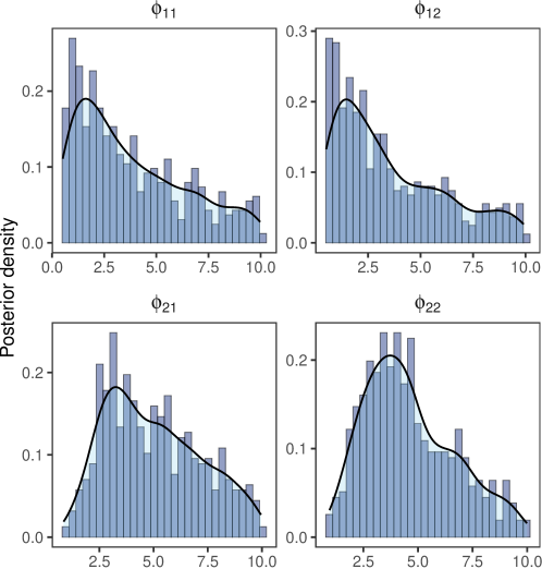
Figure A1. Histograms of posterior samples of the spatial-temporal process parameters obtained by MCMC on a fully Bayesian model on a simulated Poisson count data of sample 100.

Moreover, in addition to Fig. 1 in the main article, where we plot the posterior medians of the spatial-temporal random effects for the simulated Poisson count data, Figure A2 plots 100 quantiles of the combined posterior samples of spatial-temporal random effects obtained by stacking against quantiles obtained from MCMC. This demonstrates strong agreement between the posterior distributions obtained from the competing algorithms with most of the points concentrated along the$y=x$ line (red dashed).

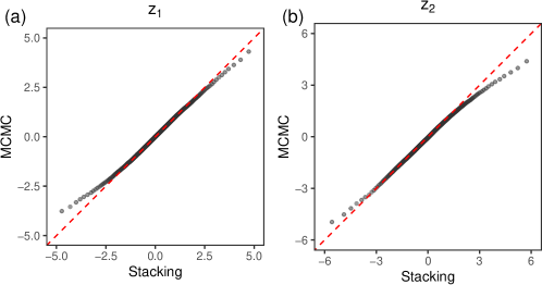
Figure A2. Plot of quantiles of the posterior distributions of the spatial-temporal random effects corresponding to (a) intercept and, (b) predictor obtained by stacking against MCMC with the $y=x$ reference as a red dashed line.

We also present results from an additional simulation experiment that demonstrates posterior learning of a random field modelling the underlying spatial or spatial-temporal processes. For convenient visualisation of the random field, we consider spatial data instead of spatial-temporal data in a continuous time domain. We simulate a dataset with responses distributed as $y(s)\sim\mathrm{Poisson}(\exp(x(s)^{\top}\beta+z(s))$ with sample size 1000. The locations are sampled uniformly inside the unit square $[0,1]^{2}$. The explanatory vector $x(s)$ consists of an intercept and one predictor sampled from the standard normal distribution and the regression coefficients are taken as $\beta=(5,-0.5)$. The latent spatial process $z(s)\sim\mathrm{GP}(0,\sigma^{2}_{z}R(\cdot,\cdot;\phi,\nu))$ is a zero-centred Gaussian process with $\sigma^{2}_{z}=0.4$, $\phi=3.5$ and $\nu=0.5$, where $R(\cdot,\cdot;\phi,\nu)$ is the Matérn correlation function,

$$R(s,s^{\prime};\phi,\nu)=\frac{(\phi\lvert s-s^{\prime}\rvert)^{\nu}}{2^{\nu-1}\Gamma(\nu)}K_{\nu}(\phi\lvert s-s^{\prime}\rvert))\;,$$ (A11)

$\lvert s-s^{\prime}\rvert$ is the Euclidean distance between $s$ and $s^{\prime}$, and ${\theta_{\text{sp}}}=\{\phi,\nu\}$. The parameter $\nu>0$ controls the smoothness of the realised random field, $\phi$ is the spatial decay parameter, $\Gamma(\cdot)$ denotes the gamma function, and $K_{\nu}$ is the modified Bessel function of the second kind of order $\nu$ (Abramowitz and Stegun, 1965, Chapter 10). The model in (7) can be modified for accommodating a spatial regression by considering $r=1$ and subsequently $\tilde{X}=I_{n}$. Here, $\mathcal{S}$ is the domain of interest. We stack on the parameters $\Delta=\{\alpha_{\epsilon},\sigma_{\xi},\phi,\nu\}$ with hyperparameters $\nu_{\beta}=\nu_{z}=3$. We also implement a fully Bayesian model with uniform priors $\mathrm{U}(0.5,10)$ for $\phi$ and $\mathrm{U}(0.1,2)$ for $\nu$. We modify our adaptive Metropolis-within-Gibbs algorithm accordingly. Figure A3 compares the posterior distributions of the spatial random effects obtained by predictive stacking and MCMC with its true values. We observe indistinguishable spatial surfaces of the posterior medians of the spatial random effects.

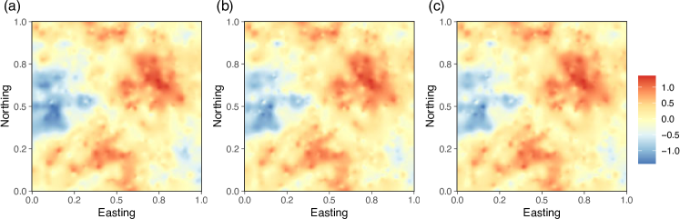
Figure A3. Comparison of interpolated surfaces of (a) the true spatial effects, with posterior median of spatial effects obtained by (b) MCMC, and, (c) our proposed predictive stacking algorithm on a simulated spatial count data.

Appendix D Additional data analysis

We offer some additional data analysis from the North American Breeding Bird Survey to supplement the results in Section 6 of the main article. In the survey, the data are collected annually during the breeding season, primarily in June, along thousands of randomly established roadside survey routes in the United States and Canada. Routes are roughly 24.5 miles (39.2 km) long with counting locations placed at approximately half-mile (800 m) intervals, for a total of 50 stops. At each stop, a citizen scientist, highly skilled in avian identification, conducts a 3-minute point count recording all birds seen within a quarter-mile (400 m) radius and all birds heard. Routes are sampled once per year. In addition to avian count data, this dataset also contains route location information including country, state and the geographic coordinates of the route start point. The variable ‘car’ records the total number of motorised vehicles passing a particular point count stop during the 3-minute count period. The variable ‘noise’ represents the presence/absence of excessive noise defined as noise from sources other than vehicles passing the survey point (e.g. from streams, construction work, vehicles on nearby roads, etc.) lasting 45 seconds that significantly interferes with the observer’s ability to hear birds at the stop during the 3-minute count period. More information on the survey can be found online at BBS 2022 data release (https://www.usgs.gov/data/2022-release-north-american-breeding-bird-survey-dataset-1966-2021).

The main article discusses the global regression coefficients. Figures A4 and A5 display side-by-side plots of the observed point counts and interpolated spatial surfaces of the posterior median of the processes assigned to the intercept and the predictors ‘car’ and ‘noise’, revealing clear spatial-temporal patterns in the effect of the predictors.

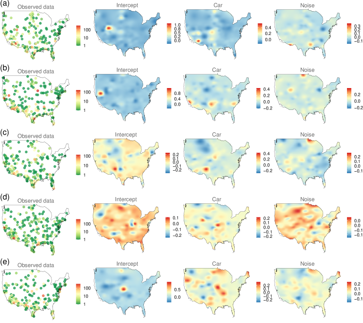
Figure A4. (a)–(e) Observed avian point count data and interpolated surfaces of posterior median of spatial-temporal random effects in the intercept as well as slopes of the variables ‘car’ and ‘noise’ for years 2010-2014.

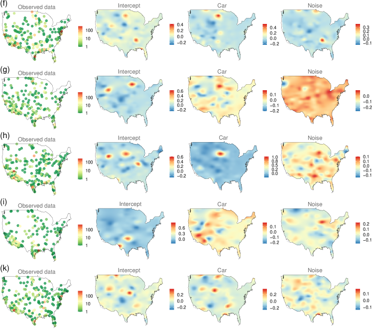
Figure A5. (f)–(k) North American Breeding Bird Survey (2015-19): Observed avian point count data and interpolated surfaces of posterior median of spatial-temporal random effects in the intercept as well as slopes of the variables ‘car’ and ‘noise’ for years 2015-2019.

References

• Abramowitz and Stegun (1965) Milton Abramowitz and Irene A. Stegun, editors. Handbook of Mathematical Functions with Formulas, Graphs and Mathematical Tables. Dover Publications, Inc., New York, 1965.
• ApS (2023) MOSEK ApS. MOSEK Rmosek package 9.3.22, 2023. URL https://docs.mosek.com/9.3/rmosek/index.html.
• Banerjee (2017) Sudipto Banerjee. High-Dimensional Bayesian Geostatistics. Bayesian Analysis, 12(2):583 – 614, 2017. doi: 10.1214/17-BA1056R.
• Banerjee et al. (2003) Sudipto Banerjee, Brad P. Carlin, and Alan E. Gelfand. Hierarchical Modeling and Analysis for Spatial Data. Chapman and Hall/CRC, 2003. doi: 10.1201/9780203487808.