Dynamical mixture modeling with fast, automatic determination of Markov chains

Abstract

Markov state modeling has gained popularity in various scientific fields due to its ability to reduce complex time series data into transitions between a few states. Yet, current frameworks are limited by assuming a single Markov chain describes the data, and they suffer an inability to discern heterogeneities. As a solution, this paper proposes a variational expectation-maximization algorithm that identifies a mixture of Markov chains in a time-series data set. The method is agnostic to the definition of the Markov states, whether data-driven (e.g. by spectral clustering) or based on domain knowledge. Variational EM efficiently and organically identifies the number of Markov chains and dynamics of each chain without expensive model comparisons or posterior sampling. The approach is supported by a theoretical analysis and numerical experiments, including simulated and observational data sets based on Last.fm music listening, ultramarathon running, and gene expression. The results show the new algorithm is competitive with contemporary mixture modeling approaches and powerful in identifying meaningful heterogeneities in time series data.

1 Introduction

To address the complexity of high-dimensional data emerging from observations and experiments, a valuable strategy involves reducing data into a small collection of states. Often, the data comes in the form of dynamical trajectories which are modeled using a finite-state Markov chain that jumps between different regions (“states”) of phase space. This modeling approach is known as Markov state modeling [1], and it has become increasingly popular in chemistry [2, 3, 4], biology [5, 6, 7, 8], and climate science [9, 10, 11] over the past two decades.

In spite of the rapid uptake and development of Markov state modeling methods, there is a limiting deficit in strategies for handling heterogeneities that plague real data sets. This paper addresses the shortcoming in the Markov state modeling literature, as it makes the following argument:

Many time-series data sets are naturally modeled as mixtures of different Markov chains, rather than a single Markov chain.

The paper proposes that Markov state modeling, which is traditionally applied to one Markov chain at a time, can be applied to learn several Markov chains simultaneously. To make this approach computationally tractable, the paper presents a Markov chain mixture modeling algorithm that automatically detects the number of Markov chains and the dynamics of each chain. This method unlocks the ability to identify heterogeneities in data sets that existing approaches would miss. Indeed, in the numerical examples in Sec. 6, the differences between the Markov chains prove to be more enlightening than any single Markov chain on its own.

The proposed algorithm is based on variational expectation-maximization [12, Sec. 10], which is a well-established tool in the statistics literature. The goal of this paper is to communicate the usefulness of variational EM for Markov chain mixture analysis. The method can be applied to states that are defined through a data-driven approach (e.g., a clustering method) or by domain knowledge.

The adaptation of variational EM for the Markov state modeling context is novel. Variational EM was previously developed for Gaussian mixture models [13, 14, 12] and hidden Markov models [15, 16, 17], but apparently this is the first paper using the method for Markov chain mixtures.

As advantages, variational EM leads to a runtime that is linear in the number of trajectories $N$ and also linear in the number of model parameters. Additionally, variational EM enables automatic detection of the number of Markov chains [14, 18, 19]. Previously, researchers would fit several Markov chain mixture models with different numbers of components and then make time-consuming model comparisons using fit statistics such as AIC or BIC [20, 21, 22]. By eliminating the need for such model comparisons, variational EM can reduce the runtime to identify $k$ Markov chains by a factor of $k$ or more.

It is important to understand the practical and theoretical limitations of any new approach. As the first limitation, the Markov state mixture model is best suited for time-series data that can be plausibly modeled as (a) finite-state and (b) Markovian. This limitation is shared with the Markov state modeling more generally.

As the second limitation, variational EM does not always converge to the globally optimal parameters. Variational EM is fast enough that randomly initializing at $10^{2}$ different parameter values is a feasible strategy that leads to high-quality solutions. Yet, future research should investigate more principled initialization for variational EM.

As the last limitation, it is impossible for a Markov chain classification algorithm to achieve high accuracy when the chains are too short. This paper establishes a new result that the Kullback-Leibler divergence fundamentally limits the reliability of Markov chain mixture modeling (see Sec. 5). The Kullback-Leibler divergence increases linearly with the trajectory length $T$, so the optimal classification rate improves exponentially with $T$. Increasing the trajectory length is the single most important factor for boosting the classification accuracy of a Markov chain mixture model.

1.1 Plan for the paper

The rest of the paper is organized as follows. Section 2 introduces Markov state modeling and Markov state mixture modeling, Section 3 reviews previous related approaches, Section 4 introduces the variational EM algorithm, Section 5 provides theoretical analysis, Section 6 presents numerical experiments, and Section 7 concludes.

1.2 Notation

Scalars are in regular typeface: $k,s,t,T,N,D$. Lowercase letters $k,s,t$ indicate scalar quantities that can vary from line to line. Uppercase letters $T,N,D$ indicate scalar quantities that are fixed by the data set.

Vectors are typically written in bold lowercase typeface: $\bm{\mu},\bm{\nu},\bm{q}$. Matrices are written in bold uppercase typeface: $\bm{K},\bm{P}$. The entries of vectors and matrices are indicated with parentheses and regular typeface: $\mu(i)$, $D(i,i)$.

Trajectories are a special class of vectors indexed by time $t=0,1,\ldots,T$ and written in uppercase bold typeface: $\bm{X},\bm{Y}$. The states of trajectories are written in regular typeface with subscripts: $X_{t},Y_{t}$. Superscripts denote trajectories in a collection: $\bm{Y}^{1},\bm{Y}^{2},\ldots,\bm{Y}^{N}$.

Finite and infinite sets are in uppercase calligraphic letters, e.g., $\mathcal{X},\mathcal{Y}$. Elements of finite sets are often in lowercase Greek letters, e.g., $\alpha,\beta\in\mathcal{Y}$.

The probability measure $\mathbb{P}$ represents a ground-truth model, while the probability measure $\hat{\mathbb{P}}$ is a data-driven estimate.

2 Extending the Markov state model

A Markov state model is a classic approach for time series analysis with a history spanning centuries [1] and recent popularity in chemistry [2, 3, 4], biology [5, 6, 7, 8], and climate science [9, 10, 11]. A Markov state model approximates time series data as a finite-state Markov chain that jumps between suitably defined “states” of the system.

A traditional Markov state model relies on three assumptions that are described in the following sections: the finite-state assumption (Sec. 2.1), the Markovian assumption (Sec. 2.2), and the one-chain assumption (Sec. 2.3). However, the one-chain assumption may be inappropriate, and Sec. 2.4 will relax the one-chain assumption and generalize the Markov state model to a Markov state mixture model.

2.1 The finite-state assumption

In a Markov state model, a dynamical system on a general state space $\mathcal{X}$ is reduced to a dynamical system on a finite state space $\mathcal{Y}=\{1,2,\ldots,s\}$. The finite states are assumed to be internally homogeneous and meaningfully different from one another. Clearly delineated states are crucial to the interpretability of the Markov state model.

There are various approaches for defining an appropriate set of finite states. As one approach, the states can be defined based on domain-area expertise. For example, user activity on MSNBC.com (“clickstreams”) can be reduced to a state space $\mathcal{Y}$ consisting of different types of webpages, such as the homepage (state 1), the news pages (state 2), and the sports pages (state 3) [22]. These state definitions are based on the MSNBC.com site map and the conventional division of articles into “sports” versus “news”.

As a more systematic alternative, the state space $\mathcal{X}$ can be decomposed using a distance function $d:\mathcal{X}\times\mathcal{X}\rightarrow\mathbb{R}$ and a set of data centers $\{\bm{c}_{1},\ldots,\bm{c}_{s}\}$. This leads to the division into cells

$$\mathcal{X}=\mathcal{X}_{1}\cup\cdots\cup\mathcal{X}_{s},\quad\text{where}$$

$$\mathcal{X}_{i}=\{\bm{x}\in\mathcal{X}:d(\bm{x},\bm{c}_{i})\leq d(\bm{x},\bm{c}_{j})\text{ for }j\neq i\}.$$

Any trajectory $\bm{X}$ on the state space $\mathcal{X}$ can be approximated by a trajectory $\bm{Y}$ on the reduced state space $\mathcal{Y}=\{1,\ldots,s\}$ by setting $Y_{t}=i$ if $X_{t}\in\mathcal{X}_{i}$ (with arbitrary tie-breaking at the boundaries).

Identifying a suitable distance function $d$ and a set of data centers $\{\bm{c}_{1},\ldots,\bm{c}_{s}\}$ can be tricky. When the data lies in $\mathcal{X}=\mathbb{R}^{D}$, one popular method combines all the trajectory locations into a data set $\{\bm{x}_{i}\}_{1\leq i\leq M}$ and selects the centers $\{\bm{c}_{1},\ldots,\bm{c}_{s}\}$ that minimize the sum of square distances

$$\sum\nolimits_{i=1}^{M}\min_{1\leq j\leq s}d(\bm{x}_{i},\bm{c}_{j})^{2}.$$

where $d(\bm{x},\bm{y})=\lVert\bm{x}-\bm{y}\rVert$ is the Euclidean distance. This method is called $k$-means clustering [23].

$k$-means clustering is common but not always effective at identifying finite states. Spectral clustering [24] is an alternative method that adapts to the nonlinear manifold structure of the input data. Spectral clustering can be applied to any state space (not just $\mathcal{X}=\mathbb{R}^{D}$), as long as there is a kernel function $k:\mathcal{X}\times\mathcal{X}\rightarrow\mathbb{R}$ which quantifies the similarity between data points. Fig.  1 illustrates spectral clustering on a spiral data set using the Gaussian kernel $k(\bm{x},\bm{y})=\exp(-\tfrac{1}{2\sigma^{2}}\lVert\bm{x}-\bm{y}\rVert^{2})$ with bandwidth $\sigma=1$. For a demonstration of spectral clustering on gene expression data, see Sec. 6.4.

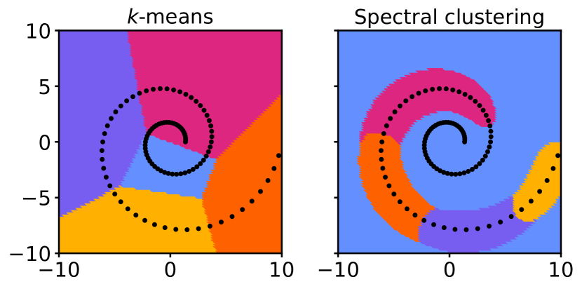
Figure 1: Comparison of $k$-means (left) versus spectral clustering (right) applied to $M=100$ data points in a spiral. Spectral clustering adapts to the nonlinear manifold structure of the data, $k$-means does not.

Algorithm 1 Spectral clustering [24]

1:Data points $\bm{x}_{1},\ldots,\bm{x}_{M}\in\mathcal{X}$, kernel function $k:\mathcal{X}\times\mathcal{X}\rightarrow\mathbb{R}$, number of states $s$, embedding dimension $r$ (default $r=s$).

2:Clusters $\mathcal{X}=\mathcal{X}_{1}\cup\cdots\cup\mathcal{X}_{s}$.

3:Evaluate the kernel matrix $\bm{K}\in\mathbb{R}^{M\times M}$ with entries $K(i,j)=k(\bm{x}_{i},\bm{x}_{j})$.

4:Evaluate the diagonal matrix $\bm{D}\in\mathbb{R}^{M\times M}$ with entries $D(i,i)=\sum\nolimits_{j=1}^{M}K(i,j)$.

5:Calculate the dominant eigenvectors of $\bm{D}^{-1/2}\bm{K}\bm{D}^{-1/2}$, and set $\bm{V}=\begin{bmatrix}\bm{v}_{1}&\cdots&\bm{v}_{r}\end{bmatrix}$.

6:Update $\bm{V}\leftarrow\bm{D}^{-1/2}\bm{V}$.

7:Define the embedding $\bm{f}:\mathcal{X}\rightarrow\mathbb{R}^{r}$ via

$$\bm{f}(\bm{x})=\sum\nolimits_{i=1}^{M}\bm{\alpha}(\cdot,i)k(\bm{x}_{i},\bm{x}),$$

where $\bm{\alpha}\in\mathbb{R}^{r\times M}$ is chosen to solve $\bm{K}\bm{\alpha}^{T}=\bm{V}$. Note the embedded data points satisfy $\bm{f}(\bm{x}_{i})=\bm{V}(i,\cdot)^{T}$ for $1\leq i\leq M$.

8:Apply $k$-means to identify centers $\bm{c}_{1},\ldots,\bm{c}_{s}\in\mathbb{R}^{r}$ for the embedded data points.

9:Define clusters by

$$\mathcal{X}_{i}=\bigl{\{}\bm{x}\colon\lVert\bm{f}(\bm{x})-\bm{c}_{i}\rVert\leq\lVert\bm{f}(\bm{x})-\bm{c}_{j}\rVert\text{ for }j\neq i\bigr{\}}.$$

Alg. 1 provides simple, direct pseudocode for spectral clustering that emphasizes the cluster definitions. However, the pseudocode becomes prohibitively slow when the data size $M$ is large. For such cases, there is a faster spectral clustering implementation in [25] that reduces the cost from $\mathcal{O}(M^{2})$ operations to $\mathcal{O}(M)$ operations.

2.2 The Markovian assumption

In a Markov state model, each trajectory $\bm{Y}$ is assumed to be Markovian. The Markovian assumption means that the position $Y_{t}$ depends only on the immediate past position $Y_{t-1}$, regardless of all the earlier positions $Y_{t-2},Y_{t-3},\ldots$. Thus, all the transition probabilities can be written as

$$\mathbb{P}\{Y_{t}=\beta\,|\,Y_{0}=\alpha_{0},\ldots,Y_{t-1}=\alpha_{t-1}\}=P(\alpha,\beta),$$

for a suitable transition matrix $\bm{P}\in\mathbb{R}^{s\times s}$.

Like all model assumptions, the Markovian assumption is an idealization of the truth. Many dynamical systems are not precisely Markovian because they exhibit prolonged history effects [26]. As an example of history dependence, consider the travel patterns of adults in Nanjing, China [27]. On a given day, a parent is unlikely to commute to their child’s school more than twice (first taking the child to school, second picking the child up from school). Because of this history dependence, the location of the adult during the day does not precisely form a Markov chain. Nonetheless, a rich and detailed description of the daily lives of residents is possible using the Markov chain assumption [27]. In general, a Markov state model assumes that history effects can be disregarded while still providing a meaningful analysis.

2.3 The one-chain assumption

The final assumption of a Markov state model is rarely stated yet fundamental. The standard presentations of Markov state modeling [28, 29, 1] all tacitly assume that a single Markov chain generates the trajectories. If the data set consists of multiple trajectories $\bm{Y}^{1},\bm{Y}^{2},\ldots,\bm{Y}^{n}$, the trajectories are all assumed to be generated from the same transition matrix $\bm{P}$.

The one-chain assumption is well-justified if the trajectories are computer simulations from a fixed model. Yet, the one-chain assumption becomes strained when faced with the heterogeneities of real-world observations. For example, is there really one type of web user on MSNBC.com? Is there really one type of commuter in Nanjing, China? Several papers in the statistics literature go beyond the one-chain assumption and instead they analyze MSNBC.com [22] users and Nanjing commuters [27] using a mixture of Markov chains with distinct transition matrices $\bm{P}_{1},\ldots,\bm{P}_{k}$. The resulting Markov chain mixture model will be described in the next section, and it will be the focus of the remainder of the paper.

2.4 The Markov chain mixture model

The Markov chain mixture model was presented in the papers [21, 30, 31], and it has been applied in areas including consumer behavior [22, 27], biology [32, 33], psychology [34], and economics [35]. However, the mixture model has apparently not been used in the Markov state modeling literature [28, 29, 1], which assumes a single Markov chain.

In the Markov chain mixture model, each trajectory $\bm{Y}$ is generated as follows:

$$\mathbb{P}\{Z=i\} =\mu(i),$$ (1)

$$\mathbb{P}\{Y_{0}=\alpha\,|\,Z=i\} =\nu_{i}(\alpha),$$

$$\mathbb{P}\{Y_{t}=\beta\,|\,Z=i,\,Y_{t-1}=\alpha\} =P_{i}(\alpha,\beta).$$

The variable $Z\in\{1,\ldots,k\}$ is a latent variable indicating the Markov chain label. $\mu(i)$ describes the probability of observing each label $Z=i$. The vectors $\bm{\nu}_{i}\in[0,1]^{s}$ and matrices $\bm{P}_{i}\in[0,1]^{s\times s}$ give the initialization probabilities and transition probabilities for the Markov chain with label $Z=i$. The total number of free parameters in the model is $ks^{2}-1$, and typical parameter values are $k=10^{0}$–$10^{2}$ and $s=10^{0}$–$10^{2}$.

3 Past algorithms for Markov chain mixtures

This section discusses past algorithms for fitting the parameters in a Markov chain mixture model, and it emphasizes two main themes. First, many researchers rely on the expectation-maximization (EM) algorithm for parameter inference (Sec. 3.1). Second, researchers have identified the key importance of the trajectory length $T$ for ensuring classification accuracy (Sec. 3.2).

3.1 The expectation-maximization algorithm

In several applications of Markov chain mixture modeling, the expectation-maximization (EM) algorithm gives fast and reliable parameter estimates [21, 30, 22, 27], especially when it is initialized carefully [36, 37, 38]. Alg. 2 provides a standard implementation of the EM algorithm for Markov chain mixtures. The algorithm iteratively refines the parameter estimates $\hat{\bm{\mu}}$, $\hat{\bm{\nu}}_{i}$, $\hat{\bm{P}}_{i}$, $\hat{Z}^{i}$, and outputs the converged values.

Algorithm 2 EM Algorithm [39]

1:Trajectories $(\bm{Y}^{n})_{1\leq n\leq N}$ and initial estimates $\hat{\mathbb{P}}\{Z^{n}=i\}$.

2:Refined parameter estimates $\hat{\bm{\mu}}$, $\hat{\bm{\nu}}_{i}$, $\hat{\bm{P}}_{i}$ and component labels $\hat{Z}^{n}\in\{1,\ldots,k\}$.

3:For each $n=1,\ldots,N$, form

$$U^{n}(\alpha) =\mathds{1}\{Y_{0}^{n}=\alpha\},$$

$$V^{n}(\alpha,\beta) =\sum\nolimits_{t=0}^{T-1}\mathds{1}\{Y_{t}^{n}=\alpha,\,Y_{t+1}^{n}=\beta\},$$

where $\mathds{1}\{\mathsf{S}\}$ is the function that takes the value 1 on set $\mathsf{S}$ and the value 0 otherwise.

4:for $t=1,2,\ldots$ do

5:     Update probabilities

$$\hat{\mu}(i) =\sum\nolimits_{n=1}^{N}\hat{\mathbb{P}}\{Z^{n}=i\},$$

$$\hat{\nu}_{i}(\alpha) =\sum\nolimits_{n=1}^{N}\hat{\mathbb{P}}\{Z^{n}=i\}\,V^{n}(\alpha),$$

$$\hat{P}_{i}(\alpha,\beta) =\sum\nolimits_{n=1}^{N}\,\hat{\mathbb{P}}\{Z^{n}=i\}V^{n}(\alpha,\beta).$$

6:     Rescale probabilities so $\sum_{i=1}^{k}\hat{\mu}(i)=1$, $\sum_{\alpha=1}^{s}\hat{p}_{i}(\alpha)=1$, and $\sum_{\beta=1}^{s}\hat{p}_{i}(\alpha,\beta)=1$.

7:     Compute probabilities $\hat{\mathbb{P}}\{Z^{n}=i\}$ via

$$\frac{\hat{\mu}(i)}{C_{n}}\prod_{\alpha=1}^{s}\hat{\nu}_{i}(\alpha)^{U^{n}(\alpha)}\prod_{\alpha,\beta=1}^{s}\hat{p}_{i}(\alpha,\beta)^{V^{n}(\alpha,\beta)},$$

and choose $C_{n}$ so that $\sum_{i=1}^{k}\hat{\mathbb{P}}\{Z^{n}=i\}=1$.

8:     Calculate log likelihood $\mathcal{L}=\sum\nolimits_{n=1}^{N}\log C_{n}$.

9:     Break if $|\Delta\mathcal{L}|<10^{-12}\cdot NT$.

10:end for

11:Return the estimates $\{\hat{\bm{\mu}},\hat{\bm{\nu}}_{i},\hat{\bm{P}}_{i}\}$ and labels $\hat{Z}^{n}=\operatorname{argmax}_{1\leq i\leq k}\hat{\mathbb{P}}\{Z^{n}=i\}$.

As a limitation, EM is a nonconvex optimization algorithm that can converge to spurious local maxima in the likelihood landscape. Therefore, the accuracy of the EM parameter estimates depends on the initialization values, which can be chosen either randomly [22, 27] or by a more structured approach [21, 37, 38, 36]. In a random initialization, the user can generate probability estimates $\hat{\mathbb{P}}\{Z^{n}=i\}$ for $i=1,\ldots,k$ that are uniformly distributed on the probability simplex. A convenient procedure for generating uniformly distributed vectors on the simplex is to first produce $k$ independent exponential random variables and then normalize them to sum to one [40].

As another limitation, EM does not automatically determine the number of mixture components. Rather, the number of components must be specified as input, and determining the best number of components requires fitting various models and then performing a comparison using AIC or BIC [20, 21, 22]. This procedure can multiply the runtime by a factor of $k$ or more, assuming the user searches over $k$ different models. Sec. 4 will present an improvement of the EM algorithm called variational EM (VEM) that does automatically determine the number of components.

3.2 The trajectory length $T$

The second theme in the Markov chain mixture modeling literature is the close link between the classification accuracy and the trajectory length $T$. Put simply, classifying short trajectories with the correct labels is hard. For example, Ramoni and coauthors [30, Sec. 5.3.1] describe numerical experiments with increasing trajectory lengths that lead to steadily increasing accuracy.

Researchers have tackled the issue of trajectory length by focusing on the extremes of short trajectories ($T=3$, [37, 38]) or long trajectories ($T\rightarrow\infty$, [41, 42, 36]). As the result of these investigations, there are now structured initializations for EM that use short trajectories of length $T=3$ [37, 38], but these approaches require massive amounts of data ($N=10^{8}$ trajectories to achieve classification error $<10\%$ [37]). At the other extreme, there are initialization algorithms for EM that ensure perfect parameter identification in the limit $T\rightarrow\infty$ [41, 36].

Sec. 5 provides further insight into the intermediate regimes where $T$ is neither short nor long. There is a nonasymptotic bound on the classification error which is valid for any Markov chain mixture model with any trajectory length $T$. The new bound indicates the importance of long trajectories, since the trajectory length leads to greater separation in Kullback-Leibler divergence and exponentially higher classification accuracy.

4 Variational EM algorithm for Markov chain mixtures

This paper proposes an extension of the variational EM algorithm, which can be used to model any time-series data set as a mixture of finite-state Markov chains. The current section describes the new method in detail and describes the steps needed for any user to apply the method to data.

As the first conceptual step, the user must reduce the data to a finite state space $\mathcal{Y}=\{1,\ldots,s\}$. The states can be chosen based on domain-area expertise or based on spectral clustering (Alg. 1), as is common in the Markov state modeling literature. The typical number of states is $s=10^{0}$–$10^{2}$.

Next, the user must choose the maximum number of mixture components, typically $k=10^{1}$–$10^{2}$. As long as $k\geq k_{\mathrm{true}}$, the approach is capable of identifying the true number of components. However, there is motivation to not set $k$ too large, as the computational cost is proportional to $k$.

The data set is then described using the Bayesian mixture model:

$$\bm{\mu} \sim\operatorname{Dir}(\bm{1}_{k}/k),$$ (2)

$$\bm{\nu}_{i} \sim\operatorname{Dir}(\bm{1}_{s}),$$

$$\bm{P}_{i}(\alpha\,\cdot) \sim\operatorname{Dir}(\bm{1}_{s}),$$

$$\mathbb{P}\{Z=i\} =\mu(i),$$

$$\mathbb{P}\{Y_{0}=\alpha\,|\,Z=i\} =\nu_{i}(\alpha),$$

$$\mathbb{P}\{Y_{t}=\beta\,|\,Z=i,\,Y_{t-1}=\alpha\} =P_{i}(\alpha,\beta).$$

This model is newly presented here, but it combines standard Bayesian formulations for a Markov state model [43] and a general mixture model [44]. The model places uninformative $\operatorname{Dir}(\bm{1}_{s})$ prior distributions on the parameters $\bm{\nu}_{i}$ and the rows of the matrix $\bm{P}_{i}(\alpha,\cdot)$. The model places a different $\operatorname{Dir}(\bm{1}_{k}/k)$ prior distribution on the mixture parameters $\bm{\mu}$. This prior distribution is theoretically and empirically motivated, as it leads to a posterior distribution that automatically prunes extraneous mixture components by setting the corresponding mixture probabilities to $\mu(i)\approx 0$ [45, 19, 46].

Given the model (2) and the observed trajectories, the Bayesian posterior distribution is hard to compute exactly. However, the posterior can be efficiently approximated by a factorized distribution (see [12, Sec. 10.2]):

$$\mathbb{P}(\{Z^{n},\bm{\mu},\bm{\nu}_{i},\bm{P}_{i}\})\approx Q_{1}(\{Z^{n}\})\cdot Q_{2}(\{\bm{\mu},\bm{\nu}_{i},\bm{P}_{i}\}).$$

This factorization assumes the latent variables $\{Z^{n}\}$ are independent from the mixture parameters $\{\bm{\mu},\bm{\nu}_{i},\bm{P}_{i}\}$. Given this factorization, the best approximation that minimizes the Kullback-Leibler divergence with respect to the posterior is a sequence of mutually independent random variables:

$$\bm{Z}^{n} \sim\operatorname{Mult}(\bm{\gamma}^{n}),$$ (3)

$$\bm{\mu} \sim\operatorname{Dir}(\bm{N}),$$

$$\bm{\nu}_{i} \sim\operatorname{Dir}(\bm{N}_{i}),$$

$$\bm{P}_{i}(\alpha,\cdot) \sim\operatorname{Dir}(\bm{N}_{i,\alpha}).$$

These random variables can be calculated using the variational EM algorithm in Alg. 3.

Algorithm 3 Variational EM Algorithm

1:Trajectories $\bm{Y}^{n}$, estimates $\hat{\mathbb{P}}\{Z^{n}=i\}$.

2:Refined estimates $\hat{\bm{N}},\hat{\bm{N}}_{i},\hat{\bm{N}}_{i,\alpha},\hat{Z}^{n}$.

3:For each $n=1,\ldots,N$, form

$$U^{n}(\alpha) =\mathds{1}\{Y_{0}^{n}=\alpha\},$$

$$V^{n}(\alpha,\beta) =\sum\nolimits_{0\leq t\leq T-1}\mathds{1}\{Y_{t}^{n}=\alpha,\,Y_{t+1}^{n}=\beta\}.$$

4:for $t=1,2,\ldots$ do

5:     Compute Dirichlet parameters

$$\hat{N}(i) =\frac{1}{k}+\sum\nolimits_{n=1}^{N}\hat{\mathbb{P}}\{Z^{n}=i\},$$

$$\hat{N}_{i}(\alpha) =1+\sum\nolimits_{n=1}^{N}\hat{\mathbb{P}}\{Z^{n}=i\}\,U^{n}(\alpha),$$

$$\hat{N}_{i,\alpha}(\beta) =1+\sum\nolimits_{n=1}^{N}\,\hat{\mathbb{P}}\{Z^{n}=i\}V^{n}(\alpha,\beta).$$

6:     Compute vectors $\hat{\bm{\mu}}$, $\hat{\bm{\nu}}_{i}$, $\hat{\bm{P}}_{i}(\alpha,\cdot)$ via

$$\log\hat{\mu}(i) =\psi(\hat{N}(i))-\psi\Bigl{(}\sum\nolimits_{j=1}^{k}\hat{N}(j)\Bigr{)},$$

$$\log\hat{\nu}_{i}(\alpha) =\psi(\hat{N}_{i}(\alpha))-\psi\Bigl{(}\sum\nolimits_{\beta=1}^{s}\hat{N}_{i}(\beta)\Bigr{)},$$

$$\log\hat{P}_{i}(\alpha,\beta) =\psi(\hat{N}_{i,\alpha}(\beta))-\psi\Bigl{(}\sum\nolimits_{\gamma=1}^{s}\hat{N}_{i,\alpha}(\gamma)\Bigr{)}.$$

$\psi(x)=\frac{d}{dx}\log\Gamma(x)$ is the digamma function.

7:     Update probabilities $\hat{\mathbb{P}}\{Z^{n}=i\}$ via

$$\frac{\hat{\mu}(i)}{C_{n}}\prod\nolimits_{\alpha=1}^{s}\hat{\nu}_{i}(\alpha)^{U^{n}(\alpha)}\prod\nolimits_{\alpha,\beta=1}^{s}\hat{P}_{i}(\alpha,\beta)^{V^{n}(\alpha,\beta)},$$

and choose $C_{n}$ so that $\sum\nolimits_{1\leq i\leq k}\hat{\mathbb{P}}\{Z^{n}=i\}=1$.

8:     Calculate variational lower bound

$$\mathcal{L} =\sum_{n=1}^{N}\log C_{n}+\log\biggl{[}\frac{B(\bm{1}_{k}/k)}{B(\hat{\bm{N}})}\prod_{i=1}^{k}\hat{\mu}_{i}^{\hat{N}(i)-1/k}\biggr{]}$$

$$+\sum_{i=1}^{k}\log\biggl{[}\frac{B(\bm{1}_{s})}{B(\hat{\bm{N}}_{i})}\prod_{\alpha=1}^{s}\hat{p}_{i}(\alpha)^{\hat{N}_{i}(\alpha)-1}\biggr{]}$$

$$+\sum_{i=1}^{k}\sum_{\alpha=1}^{s}\log\biggl{[}\frac{B(\bm{1}_{s})}{B(\hat{\bm{N}}_{i,\alpha})}\prod_{\beta=1}^{s}\hat{p}_{i,\alpha}(\beta)^{\hat{N}_{i,\alpha}(\beta)-1}\Biggr{]},$$

where $B(\bm{N})=(\prod_{i}\Gamma(N_{i}))\,/\,\Gamma(\sum_{i}N_{i})$.

9:     Break if $|\Delta\mathcal{L}|<10^{-12}\cdot NT$.

10:end for

11:Return $\hat{\bm{N}},\hat{\bm{N}}_{i},\hat{\bm{N}}_{i,\alpha},\hat{Z}^{n}=\operatorname*{argmax}\limits_{1\leq i\leq k}\hat{\mathbb{P}}\{Z^{n}=i\}$.

Examining Alg. 3, there are a couple of key changes from the standard EM algorithm (Alg. 2). First, the user receives information about the parameter $\{\bm{\mu},\bm{\nu}_{i},\bm{P}_{i}\}$ in the form of Dirichlet distributions, which encode uncertainty information about the parameters. The user can extract a point estimate for any parameter by using the mean formula for the Dirichlet distribution, e.g.,

$$\hat{\mu}(i)=\mathbb{E}[\mu(i)]=\frac{N(i)}{\sum_{j=1}^{k}N(j)}.$$ (4)

The user can also extract error bars by using the variance formula for the Dirichlet distribution, e.g.,

$$\operatorname{Var}[\mu(i)]=\frac{N(i)\sum_{j\neq i}N(j)}{\bigl{(}\sum_{j=1}^{k}N(j)\bigr{)}^{2}\bigl{(}\sum_{j=1}^{k}N(j)+1\bigr{)}}.$$

The automatic availability of uncertainty information is a helpful feature of the Bayesian approach.

As the second change, variational EM automatically determines the number of mixture components. Upon convergence, only a small number of mixture parameters satisfy $\hat{N}(i)\geq 1$. The optimization drives all the remaining mixture parameters to the lowest possible value $\hat{N}(i)=1/k$. These components are not represented by any labels $\hat{Z}^{n}=i$, so they are effectively removed from the model. The tendency of variational EM to identify a parsimonious mixture model is called automatic relevance determination. It was observed heuristically in the papers [14, 18] and later justified based on asymptotic arguments in [19].

To apply Alg. 3 in practice, the user needs some way to initialize the parameter estimates. Since there is limited theoretical understanding of the best way to initialize variational EM, this paper uses a random sampling technique. The algorithm is by default run with $10^{2}$ independent initializations based on randomly sampling parameters $\hat{\mathbb{P}}\{Z^{n}=i\}$ for $i=1,\ldots,k$ from the probability simplex. After running Alg. 3 with different initializations, the user selects the optimal parameters $\{\hat{\bm{N}},\hat{\bm{N}}_{i},\hat{\bm{N}}_{i,\alpha},\hat{Z}^{n}\}$ that maximize the likelihood bound $\mathcal{L}$.

5 Limits on Markov chain mixture modeling

Markov chain mixture modeling cannot succeed when the trajectories are too short. This section provides a theoretical explanation for the high misclassification rate by presenting and interpreting the following theorem.

Theorem 1 (Misclassification error bound).

Consider any statistical estimator $\hat{Z}$ for the label $Z$ in the Markov chain mixture model (1). The estimator can depend on the observed data $\bm{Y}$ and the model parameters but not on the unknown label $Z$. Then, the misclassification error is at least

$$\mathbb{P}\{\hat{Z}\neq Z\}\geq\frac{1}{2}\sum_{i=1}^{k}\max_{j\neq i}\frac{{\rm e}^{-\operatorname{D}_{\rm KL}(\mathbb{P}_{i}\,\|\,\mathbb{P}_{j})}}{\mu(i)^{-1}+\mu(j)^{-1}}.$$

In this expression, the Kullback-Leibler divergence is defined as

$$\operatorname{D}_{\rm KL}(\mathbb{P}_{i}\,\|\,\mathbb{P}_{j})=\sum_{\bm{Y}}\mathbb{P}_{i}(\bm{Y})\log\biggl{(}\frac{\mathbb{P}_{i}(\bm{Y})}{\mathbb{P}_{j}(\bm{Y})}\biggr{)}.$$

The summation runs over all possible trajectories of length $T$, and

$$\mathbb{P}_{i}(\alpha_{0},\ldots,\alpha_{T})=\nu_{i}(\alpha_{0})\prod\nolimits_{t=0}^{T-1}P_{i}(\alpha_{t},\alpha_{t+1}).$$

is the probability of observing the trajectory $\bm{Y}=(\alpha_{0},\ldots,\alpha_{T})$ given that $Z=i$.

Proof.

Given the observed data $\bm{Y}$, the conditional distribution of the component label $Z$ is

$$\mathbb{P}\{Z=i\,|\,\bm{Y}\}=\frac{\mu(i)\mathbb{P}_{i}(\bm{Y})}{\sum_{j=1}^{k}\mu(j)\mathbb{P}_{j}(\bm{Y})}.$$ (5)

The optimal classification algorithm selects the labels according to

$$\hat{Z}\in\operatorname*{argmax}_{1\leq i\leq k}\mathbb{P}\{Z=i\,|\,\bm{Y}\},$$

and the resulting statistical error is quantified by

$$\mathbb{P}\{Z\neq\hat{Z}\,|\,\bm{Y}\}=1-\max_{1\leq i\leq k}\mathbb{P}\{Z=i\,|\,\bm{Y}\}.$$

Next, use the inequality $1-\alpha\geq(1-\alpha^{2})/2$ to obtain the lower bound

$$\mathbb{P}\{Z\neq\hat{Z}\,|\,\bm{Y}\}$$

$$=1-\max_{1\leq i\leq k}\mathbb{P}\{Z=i\,|\,\bm{Y}\}$$

$$\geq\frac{1}{2}-\frac{1}{2}\max_{1\leq i\leq k}\mathbb{P}\{Z=i\,|\,\bm{Y}\}^{2}$$

$$\geq\frac{1}{2}-\frac{1}{2}\sum\nolimits_{i=1}^{k}\mathbb{P}\{Z=i\,|\,\bm{Y}\}^{2}$$

$$=\frac{1}{2}\sum\nolimits_{i=1}^{k}\mathbb{P}\{Z=i\,|\,\bm{Y}\}(1-\mathbb{P}\{Z=i\,|\,\bm{Y}\}).$$

Multiply both sides by $\mathbb{P}(\bm{Y})$ and sum over all possible trajectories $\bm{Y}$ to obtain the formula

$$\mathbb{P}\{Z\neq\hat{Z}\}=\sum\nolimits_{\bm{Y}}\mathbb{P}\{Z\neq\hat{Z}\,|\,\bm{Y}\}$$ (6)

$$\geq\frac{1}{2}\sum\nolimits_{i,\bm{Y}}\mathbb{P}\{Z=i,\bm{Y}^{n}\}(1-\mathbb{P}\{Z=i\,|\,\bm{Y}\})$$

$$=\frac{1}{2}\sum\nolimits_{i=1}^{k}\mu(i)\,\mathbb{E}\bigl{[}1-\mathbb{P}\{Z=i\,|\,\bm{Y}\}\,|\,Z=i\bigr{]}.$$

The expression above turns out to be analytically tractable and is the key to the analysis.

The rest of the proof is based on bounding $\mathbb{E}\bigl{[}1-\mathbb{P}\{Z=i\,|\,\bm{Y}\}\,|\,Z=i\bigr{]}$ from below using the Kullback-Leibler divergence. To obtain a convenient lower bound, use eq. (5) to derive

$$\mathbb{E}\bigl{[}1-\mathbb{P}\{Z=i\,|\,\bm{Y}\}\,|\,Z=i\bigr{]}$$

$$=\mathbb{E}\Biggl{[}\frac{\sum_{j\neq i}\mu(j)\mathbb{P}_{j}(\bm{Y})}{\sum_{j=1}^{k}\mu(j)\mathbb{P}_{j}(\bm{Y})}\,\bigg{|}\,Z=i\Biggr{]}$$

$$\geq\mathbb{E}\biggl{[}\frac{\mu(j)\mathbb{P}_{j}(\bm{Y})}{\mu(i)\mathbb{P}_{i}(\bm{Y})+\mu(j)\mathbb{P}_{j}(\bm{Y})}\,\bigg{|}\,Z=i\biggr{]},$$

for each $j\neq i$. The inequality is due to the fact that $f(x)=x/(c+x)$ is an increasing function of $x>0$, for any $c>0$. Next, by an application of Jensen’s inequality,

$$\log\biggl{(}\mathbb{E}\biggl{[}\frac{\mu(j)\mathbb{P}_{j}(\bm{Y})}{\mu(i)\mathbb{P}_{i}(\bm{Y})+\mu(j)\mathbb{P}_{j}(\bm{Y})}\,\bigg{|}\,Z=i\biggr{]}\biggr{)}$$

$$\geq\mathbb{E}\biggl{[}\log\biggl{(}\frac{\mu(j)\mathbb{P}_{j}(\bm{Y})}{\mu(i)\mathbb{P}_{i}(\bm{Y})+\mu(j)\mathbb{P}_{j}(\bm{Y})}\biggr{)}\,\bigg{|}\,Z=i\biggr{]}$$

$$\begin{aligned} &=\mathbb{E}\biggl{[}\log\biggl{(}\frac{\mathbb{P}_{j}(\bm{Y})}{\mathbb{P}_{i}(\bm{Y})}\biggr{)}\,\bigg{|}\,Z=i\biggr{]}\\ &\quad-\mathbb{E}\biggl{[}\log\biggl{(}\frac{\mu(i)}{\mu(j)}+\frac{\mathbb{P}_{j}(\bm{Y})}{\mathbb{P}_{i}(\bm{Y})}\biggr{)}\,\bigg{|}\,Z=i\biggr{]}.\end{aligned}$$

The first term in the final expression is the negative Kullback-Leibler divergence

$$\mathbb{E}\biggl{[}\log\biggl{(}\frac{\mathbb{P}_{j}(\bm{Y})}{\mathbb{P}_{i}(\bm{Y})}\biggr{)}\,\bigg{|}\,Z=i\biggr{]}=-\operatorname{D}_{\rm KL}(\mathbb{P}_{i}\,\|\,\mathbb{P}_{j}).$$

The second term can be bounded by another application of Jensen’s inequality:

$$-\mathbb{E}\biggl{[}\log\biggl{(}\frac{\mu(i)}{\mu(j)}+\frac{\mathbb{P}_{j}(\bm{Y})}{\mathbb{P}_{i}(\bm{Y})}\biggr{)}\,\bigg{|}\,Z=i\biggr{]}$$

$$\geq-\log\biggl{(}\frac{\mu(i)}{\mu(j)}+\mathbb{E}\biggl{[}\frac{\mathbb{P}_{j}(\bm{Y})}{\mathbb{P}_{i}(\bm{Y})}\,\bigg{|}\,Z=i\biggr{]}\biggr{)}.$$

Moreover, observe that

$$\mathbb{E}\biggl{[}\frac{\mathbb{P}_{j}(\bm{Y})}{\mathbb{P}_{i}(\bm{Y})}\,\bigg{|}\,Z=i\biggr{]} =\sum\nolimits_{\bm{Y}}\mathbb{P}_{i}(\bm{Y})\frac{\mathbb{P}_{j}(\bm{Y})}{\mathbb{P}_{i}(\bm{Y})}$$

$$=\sum\nolimits_{\bm{Y}}\mathbb{P}_{j}(\bm{Y})=1.$$

Tying together the above expressions, it follows

$$\mathbb{E}\bigl{[}1-\mathbb{P}\{Z=i\,|\,\bm{Y}\}\,|\,Z=i\bigr{]}\geq\max_{j\neq i}\frac{{\rm e}^{-\operatorname{D}_{\rm KL}(\mathbb{P}_{i}\,\|\,\mathbb{P}_{j})}}{\frac{\mu(i)}{\mu(j)}+1}.$$

Combine with eq. (6) to complete the proof. ∎

Thm. 1 determines the theoretical limits on classification accuracy in terms of the Kullback-Leibler divergence. The theorem extends to general mixture models, and it is apparently new in the statistics literature.

To interpret the theorem, it is instructive to consider what happens to the KL divergence as the trajectory length $T$ approaches infinity. If the Markov chain $i$ has a unique stationary measure $\bm{\pi}_{i}\in[0,1]^{s}$, then in the limit $T\rightarrow\infty$ the ergodic theorem for Markov chains [47, Sec. 1.10] guarantees

$$\tfrac{1}{T}\operatorname{D}_{\rm KL}(\mathbb{P}_{i}\,\|\,\mathbb{P}_{j})$$

$$=\frac{1}{T}\sum_{\alpha_{0},\ldots,\alpha_{T}}\mathbb{P}_{i}(\alpha_{0},\ldots,\alpha_{T})\log\biggl{(}\frac{\mathbb{P}_{i}(\alpha_{0},\ldots,\alpha_{T})}{\mathbb{P}_{j}(\alpha_{0},\ldots,\alpha_{T})}\biggr{)}$$

$$\rightarrow\sum\nolimits_{\alpha,\beta=1}^{s}\pi(\alpha)p_{i}(\alpha,\beta)\log\biggl{(}\frac{p_{i}(\alpha,\beta)}{p_{j}(\alpha,\beta)}\biggr{)}$$

$$=\sum\nolimits_{\alpha=1}^{s}\pi(\alpha)\operatorname{D}_{\rm KL}(p_{i}(\alpha,\cdot)\,\|\,p_{j}(\alpha,\cdot)).$$

By this derivation, the KL divergence $\operatorname{D}_{\rm KL}(\mathbb{P}_{i}\,\|\,\mathbb{P}_{j})$ is approximately $T$ times the averaged Kullback-Leibler divergence $\operatorname{D}_{\rm KL}(p_{i}(\alpha,\cdot)\,\|\,p_{j}(\alpha,\cdot))$ over all the states. The linear dependence of the Kullback-Leibler divergence on $T$ motivates the following rule of thumb. If the trajectory length doubles, the KL divergence doubles, and the misclassification rate squares. For example, doubling the length of a trajectory can reduce the misclassification rate from $1$-in-$10$ to just $1$-in-$100$.

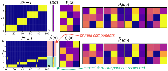
Figure 2: True parameters and parameter estimates for simulated trajectories with $k_{\mathrm{true}}=4$, $s=3$, $N=100$, and $T=30$. Top row shows true parameters. Bottom row shows parameter estimates from variational EM with a maximum of $k=10$ components. Even with limited data, VEM correctly identifies the number of components.

6 Numerical experiments

This section describes four numerical experiments with the variational EM algorithm. The first experiment (Sec. 6.1) uses simulated Markov chain data. The middle two experiments (Secs. 6.2 and  6.3) use real-world observations. The last experiment (Sec. 6.4) uses simulated genetics data. Code to run the experiments is available at https://github.com/chris-miles/MarkovChain-VEM.

6.1 Simulated Markov chain data

The first experiment is based on simulations of the Markov chain mixture model (1) with uniformly random parameters $\bm{\mu}$, $\bm{\nu}_{i}$, and $\bm{P}_{i}$. The goal of the experiment is to test whether variational EM correctly identifies the number of components and correctly classifies trajectories into components.

As the first result, variational EM accurately identifies the number of components even with a relatively small data set. Fig. 2 shows the true parameters (top) and parameter estimates (bottom) when $k_{\mathrm{true}}=4$, $s=3$, $N=100$, and $T=30$. Although variational EM is run with a maximum number of $k=10$ components, it leads to a fitted model with just 4 components. The algorithm assigns no trajectories to 6 of the 10 components, thereby pruning them from the model. The automatic identification of the number of mixture components is a major advantage compared to previous Markov chain mixture modeling approaches [20, 21, 22].

The reader may wonder, is there a cost to setting the value of $k$ excessively high? While there is an obvious computational burden to setting $k>k_{\mathrm{true}}$, the results in Fig.  3 show that the classification accuracy, defined by

$$\operatorname{acc}=\frac{1}{N}\sum\nolimits_{n=1}^{N}\mathds{1}\{Z^{n}=\hat{Z}^{n}\},$$ (7)

is not hindered. Indeed, the results with $k=4=k_{\mathrm{true}}$ (top panel) are nearly identical to results with $k=10>k_{\mathrm{true}}$ (bottom panel).

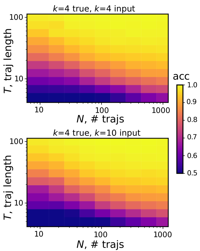
Figure 3: Classification accuracy with $k_{\mathrm{true}}=4$, $s=3$, and varying settings of $N$ and $T$. The accuracy is similar using $k=4$ (top) versus $k=10$ (bottom). In both plots, the accuracy is averaged over $250$ independent trials.

As the next result, Fig. 3 shows the trajectory length $T$ is a major factor determining the classification accuracy (7). The accuracy reaches a threshold for each $T$ value as $N\rightarrow\infty$, and increasing $T$ exponentially increases the threshold. These results in line with the theoretical analysis in Sec. 5, which also suggests an exponential dependence on $T$.

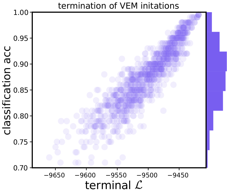
Figure 4: Demonstration of the local optima over $1000$ random variational EM initializations when $k=15$, $k_{\mathrm{true}}=10$, $s=7$, $N=100$, and $T=50$. Many variational EM runs end with nearly optimal assignments, some do not.

EM and variational EM are known to terminate in locally optimal parameter values that can be far from the global optimum [48]. To safeguard against misconvergence, this paper randomly initializes variational EM many times and accepts the results that maximize the likelihood bound $\mathcal{L}$. The outcomes of $10^{3}$ random initialization are shown in Fig. 4. For the figure, the parameters $k=15$, $k_{\mathrm{true}}=10$, $s=7$, $N=100$, and $T=50$ were deliberately chosen to make the optimization challenging and produce a range of variational EM solutions. Perfect accuracy is achieved in some variational EM runs, but other runs result in low accuracy and low $\mathcal{L}$ values. While the sensitivity of variational EM to the initial parameters may appear prohibitive, given the speed of the algorithm and its ease of parallelization, running hundreds to thousands of independent initializations is feasible and sufficient to yield reliable results. Nonetheless, there remains significant future interest in identifying more principled initializations for variational EM or more robust stochastic variants [49].

6.2 Last.fm user data

The next experiment uses a publicly available data set that records the listening histories of Last.fm users in 2007. The goal of this experiment is to compare the accuracy of variational EM against previously published Markov chain mixture modeling results [37, 36] that also analyzed the Last.fm data.

Following the previous work [36], the ground-truth model is specified as follows. There are $k_{\mathrm{true}}=10$ Markov chains, corresponding to the Last.fm users with the greatest number of song listens. There are $s=100$ state possibilities, based on assigning a discrete label to each song in a user’s listening history by the predominant genre. If a user sequentially listens to songs from the same genre, these songs are collapsed into a single state. Hence, each Markov chain models the genre transitions for a Last.fm user. To make the learning problem difficult, each user’s listening history is broken into $75$ equal-length segments, and the segments are truncated to a short trajectory length $20\leq T\leq 100$.

Figure 5: Classification accuracy for the top 10 Last.fm users, given $N=75$ trajectories and $s=100$ possible genres for each user. Top: Variational EM identifies is twice as accurate as the best method reported in [36]. Bottom: Confusion matrix for identifying the top 10 users with $T=250$.

The results in Fig. 5 show that variational EM with $k=k_{\mathrm{true}}=10$ components is twice as accurate as the best results reported in [36]. Variational EM is also more accurate than the work [37], which reports $90\%$ misclassifications on the Las.fm data set with $k_{\mathrm{true}}=10$ components. The comparison with [37] is slightly complicated however and is not reported in the figure, since the trajectories in [37] are more numerous and shorter ($N=30,000$, $T=3$).

While variational EM outperforms previous approaches, the misclassification rate for length $T=100$ trajectories is still notably high, $45\%$. To further improve the accuracy, the trajectories were extended to length $T=250$, resulting in a reduction to $30\%$ error. The right panel of Fig. 5 shows the confusion matrix, which indicates that most of the misclassifications come from 4 users who all had similar listening histories.

Figure 6: Classification of users for a Last.fm data set with $N=497$ users, $s=100$ genres, and trajectory length $T=1000$. Popular components are labeled with the most frequent genres.

For further insight, a new data set was prepared with a length $T=1000$ trajectory for each of the top $N=497$ Last.fm users. Variational EM was applied to this data set with a maximum number of $k=100$ components. Fig. 6 shows the mixture modeling results, which indicates that a few components have substantially large memberships. The 3 largest components correspond to well-known genres of ‘indie’, ‘electronic’, and ‘metal’. The overwhelming popularity of the indie component explains why distinguishing Last.fm users may be difficult. Many indie rock listeners had quite similar listening histories in 2007 [50].

6.3 Ultrarunners data set

The third experiment is based on data from the 2012 International Association of Ultrarunners (IAU) World Championship held in Katowice, Poland [51, 52]. The goal of this experiment is to determine how many pacing patterns can be observed in the data and which pacing patterns lead to the best overall performance. Conventional wisdom among ultrarunners contends that a slower pace to start is ideal [53], as many runners tend to overexert themselves during the start and tire later during a race.

Pacing is an individualized measure of performance, so each runner’s data over the 24-hour event was normalized based on their average speed. First, $12$ runners that did not complete a single lap were removed from the data set, yielding $N=248$ total trajectories. Next, each runner’s average speed was calculated by dividing the total number of laps over the 2.314km course by the total number of hours until finishing or dropping out of the event (typically 24 hours). Individualized speeds were calculated for each runner by dividing the number of laps completed each hour by the average speed. Last, the data was categorized into $s=4$ Markov states: “resting” when the hourly speed is less than $0.5$ times the average speed, “normal” when the hourly speed is between $0.5$ and $1.5$ times the average speed, “strained” when the hourly speed is greater than $1.5$ times the average speed, and a terminal “ended” state.

Figure 7: Application of Markov chain mixture modeling to the 2012 International Association of Ultrarunners (IAU) World Championship data. With a maximum of $k=10$ components, three running patterns emerged: (1) constant pace, (2) a fast start followed by subsequent resting, (3) erratic performance. Black lines show component means.

The variational EM algorithm identifies three distinct running patterns in the data, as displayed in Fig.  7. The predominant pattern ($70\%$ of runners) involves a roughly constant pace, with slightly higher relative speed at the start of the race. The second-most-common pattern ($25\%$ of runners) involves overexertion at the start of the race and a significant slowdown later. The third pattern involves erratic running with no apparent strategy. A previous analysis identified three similar running patterns in the 2012 ultrarunner data [51].

The Markov state mixture model is interesting in two ways. First, the runners in group 1 ran notably faster than those in group 2 even though the average speed was not included as input into the algorithm. Rather, a constant pace emerged organically as the top-performing pattern. Second, the ideal strategy of a slower opening pace was not observed in any group. While the slow start is considered optimal, it is also notably difficult to achieve in races [53].

6.4 Simulated gene expression data

Figure 8: Schematic of finite state approximation for the mutual-inhibition, self-activation (MISA) gene circuit. Counts of proteins $a$ and $b$ are visualized as scatter plots (column 1) and time series (column 2). $(a,b)$ trajectories are classified into 4 states (column 3), and trajectories are projected based on the 4 states (column 4). Rows indicate different magnitudes of the rate parameter $f_{r}=0.01,0.1,1.0$.

The last experiment is based on simulations of the mutual-inhibition, self-activation (MISA) gene circuit. The circuit consists of an $A$ gene and a $B$ gene that inhibit each other and activate themselves through the production of $a$ and $b$ proteins. The MISA circuit has been observed in many biological systems [54, 55, 56, 57] and studied extensively by theorists [58, 59, 60, 61]. The goal of the experiment is to test whether variational EM can correctly classify data from this biologically important system. The experiment also tests whether spectral clustering (Alg. 1) can automatically identify Markov states from the MISA data.

The MISA circuit is typically described as a chemical reaction network [62] containing the following species and reactions. There is one $A$ gene and one $B$ gene that exhibit a range of conditions $ij\in\{00,01,10,11\}$, in which they produce proteins at a rate $g_{ij}$:

$$A_{ij} \overset{g_{ij}}{\to}A_{ij}+a,\quad ij={00,01,01,11},$$

$$B_{ij} \overset{g_{ij}}{\to}B_{ij}+b,\quad ij={00,01,01,11}.$$

The rates are fixed at $g_{00}=g_{01}=g_{11}=10$ and $g_{10}=100$ since $i=1$ indicates the presence of an activator and $j=1$ indicates the presence of a repressor. The proteins degrade at rate $d=1$:

$$a\overset{d}{\to}\varnothing,\quad b\overset{d}{\to}\varnothing.$$

Last, as the proteins are produced and degrade, they influence the conditions of the $A$ and $B$ genes as follows:

$$A_{0j}+2a \stackrel{{\scriptstyle h_{a}}}{{\underset{f_{a}}{\rightleftarrows}}}A_{1j},\quad B_{0j}+2b\stackrel{{\scriptstyle h_{a}}}{{\underset{f_{a}}{\rightleftarrows}}}B_{1j},\quad j=0,1.$$

$$A_{i0}+2b \stackrel{{\scriptstyle h_{r}}}{{\underset{f_{r}}{\rightleftarrows}}}A_{i1},\quad B_{i0}+2a\stackrel{{\scriptstyle h_{r}}}{{\underset{f_{r}}{\rightleftarrows}}}B_{i1},\quad i=0,1.$$

Three of the rate parameters are fixed to $h_{a}=10^{-1}$, $f_{a}=1$, and $h_{r}=10^{-3}$. However, $f_{r}$ is a free parameter that controls the extent of protein activation versus repression in the system. In summary, the MISA gene circuit can be encoded as a vector $X_{t}\in\{00,01,10,11\}^{2}\times\mathbb{N}^{2}$, where the first two coordinates indicate conditions of the $A$ and $B$ genes and the last two coordinates indicate populations of $a$ and $b$ proteins. To generate MISA trajectories, the system $X_{t}$ was run forward in time with various values of the $f_{r}$ parameter using the stochastic simulation algorithm (SSA) implemented in PyGillespie [63]. The algorithm produces a continuous-time trajectory $(X_{t})_{t\geq 0}$; however, the states were sampled at uniformly spaced times $t=0,1,2,\ldots$ to produce a discrete-time data set.

The MISA gene circuit is interesting to biologists because of its emergent stochastic-switching behavior, which is useful in modeling cell-fate decisions [5]. Fig. 8 displays the stochastic switching in the populations of $a$ and $b$ proteins. The protein populations toggle between four metastable states, which are associated with each gene being “on” or “off”. When the rate $f_{r}$ is low (top panels), the genes are frequently off, leading to protein populations of just 0–20. When $f_{r}$ is high (bottom panels), both genes are frequently on, leading to increased populations of 50–150 proteins. The most interesting behavior occurs for intermediate values of $f_{r}$ (middle panels), because then one gene is typically on and the other is off. The genes actively compete to produce more proteins.

The MISA gene circuit is not Markovian in the protein numbers $a$ and $b$. Nonetheless, a Markov state model can be constructed by applying spectral clustering (Alg. 1) to the $(a,b)$ data. The middle panel of Fig. 8 shows the outcome of spectral clustering using a Gaussian kernel with bandwidth $\sigma=50$. The four identified clusters are interpretable and they efficiently represent the metastable dynamics.

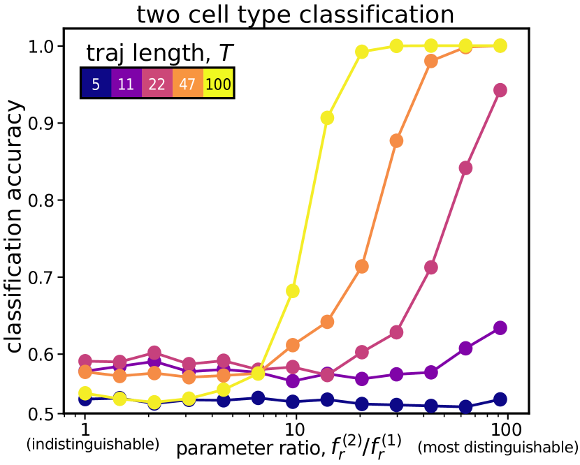
Figure 9: Classification accuracy for simulated MISA data containing 15 trajectories with $f_{r}^{(1)}=0.01$ and 15 trajectories with $f_{r}^{(2)}\neq f_{r}^{(1)}$. Trajectories are reliably identified when $T\geq 25$ and $f_{r}^{(2)}/f_{r}^{(1)}\geq 25$.

Variational EM can be used to untangle multiple Markov chains from a single MISA data set. This application area is increasingly important, as MISA models with variable parameters are now being engineered in labs [64] and applied to understand long chains of cell differentiation [56]. As an example application, researchers have obtained time series data for a MISA gene circuit in the bacteriophage $\lambda$ switch [8]. They analyzed the time-series data assuming a single Markov chain, but the Markov chain mixture model provides the ability to discern heterogeneities within the samples.

To test the feasibility of the mixture modeling approach, spectral clustering and variational EM were applied to a range of simulated MISA data sets containing $15$ trajectories with an unbinding rate $f_{r}^{(1)}=0.01$ and $15$ trajectories with a different unbinding rate $f_{r}^{(2)}\neq f_{r}^{(1)}$. The algorithms were used to untangle the two populations of trajectories, leading to the results in Fig. 9. The results indicate that the classification accuracy depends greatly on the trajectory length $T$ and the parameter ratio $f_{r}^{(2)}/f_{r}^{(1)}$. When $f_{r}^{(2)}/f_{r}^{(1)}\geq 25$ and $T\geq 25$, the populations can be separated with near-perfect accuracy. However, short trajectories with $T\leq 5$ cannot be reliably separated for any $f_{r}^{(2)}$ parameter. These results support the theoretical analysis in Thm. 1 that links the classification accuracy with the Kullback-Leibler divergence, which increases with $f_{r}^{(2)}/f_{r}^{(1)}$ and increases exponentially fast with $T$.

7 Conclusion

This paper has proposed an extension of Markov state modeling that enables the study of heterogeneities within time series data. Previous work employed Markov state modeling under the assumption that the observations come from a homogeneous population, modeled by a single Markov chain. This paper establishes the theory and practice of learning a mixture of different Markov chains simultaneously.

The paper has motivated and tested a variational EM algorithm that automatically identifies the number of chains and the dynamics of each chain. The algorithm is computationally efficient: unlike past work, it identifies the number of chains organically, without relying on expensive model comparisons or posterior sampling.

The current bottleneck, shared among all the standard methods for fitting Markov chain mixture models (EM and variational EM), is the convergence to locally optimal parameters. Running these methods with many random initializations is the currently proposed solution, but it is the computationally limiting aspect of the approach. Future work should identify and rigorously justify an initialization strategy that works well for variational EM with any trajectory length $T$.

The paper also contributes a new theorem that fundamentally limits the classification accuracy of any Markov chain classification algorithm. The bound is stated in terms of the Kullback-Leibler divergence between the underlying Markov chains, and it suggests exponentially increasing accuracy with the trajectory length $T$. This prediction is repeatedly supported in the numerical experiments (Secs. 6.1, 6.2, 6.4). The theory precisely quantifies the established wisdom [30] that long trajectories are better than short ones.

Last, there is the question of how the Markov chain mixtures can be used by scientists. Three of the four experiments (Secs. 6.2, 6.3, 6.4) were designed with applications in mind, and the method was found to yield sensible, reliable interpretations. One of the authors (C.E.M.) listened to indie rock on Last.fm in 2007 while the other author (R.J.W.) runs ultramarathons competitively, and they can attest to the qualitative accuracy of the Markov chain mixture models.

In summary, Markov chain mixture models have an established track record in distinguishing heterogeneities in human behavior, such as surfing the internet [22], commuting between home, work, and school [27], listening to music (Sec. 6.2), and running ultramarathons (Sec. 6.3). The variational EM algorithm is the best currently available strategy for fitting these models efficiently and correctly. Moving forward, there is the potential for broad utility of Markov chain mixture model in other areas (chemistry, biology, climate science) where Markov state modeling is currently popular. Indeed, the experiments in Sec. 6.4 demonstrate promising first steps toward applications in the rapidly evolving area of gene expression data analysis [65, 66, 67, 68].

Acknowledgements

The authors thank Elizabeth Read and Adam MacLean for helpful discussions about gene expression time series. C.E.M. was partially supported by a University of California Society of Hellman Fellows fund. R.J.W. was supported by the Office of Naval Research through BRC Award N00014-18-1-2363, the National Science Foundation through FRG Award 1952777, and Caltech through the Carver Mead New Adventures Fund, under the aegis of Joel A. Tropp.

Code Availability

Code to reproduce the numerical experiments can be found in the Github repository https://github.com/chris-miles/MarkovChain-VEM.

References

- \bibcommenthead
- Husic and Pande [2018] Husic, B.E., Pande, V.S.: Markov state models: From an art to a science. Journal of the American Chemical Society 140(7), 2386–2396 (2018) https://doi.org/10.1021/jacs.7b12191
- Noé et al. [2013] Noé, F., Wu, H., Prinz, J.-H., Plattner, N.: Projected and hidden Markov models for calculating kinetics and metastable states of complex molecules. The Journal of Chemical Physics 139(18), 184114 (2013) https://doi.org/10.1063/1.4828816
- Röblitz and Weber [2013] Röblitz, S., Weber, M.: Fuzzy spectral clustering by PCCA+: Application to Markov state models and data classification. Advances in Data Analysis and Classification 7(2), 147–179 (2013) https://doi.org/10.1007/s11634-013-0134-6
- Köhs et al. [2022] Köhs, L., Kukovetz, K., Rauh, O., Koeppl, H.: Nonparametric Bayesian inference for meta-stable conformational dynamics. Physical Biology 19(5), 056006 (2022) https://doi.org/10.1088/1478-3975/ac885e
- Chu et al. [2017] Chu, B.K., Tse, M.J., Sato, R.R., Read, E.L.: Markov state models of gene regulatory networks. BMC Systems Biology 11(1) (2017) https://doi.org/10.1186/s12918-017-0394-4
- Tse et al. [2018] Tse, M.J., Chu, B.K., Gallivan, C.P., Read, E.L.: Rare-event sampling of epigenetic landscapes and phenotype transitions. PLOS Computational Biology 14(8), 1–28 (2018) https://doi.org/10.1371/journal.pcbi.1006336
- Tan et al. [2019] Tan, Z.W., Guarnera, E., Berezovsky, I.N.: Exploring chromatin hierarchical organization via markov state modelling. PLOS Computational Biology 14(12), 1–35 (2019) https://doi.org/10.1371/journal.pcbi.1006686
- Fang et al. [2018] Fang, X., Liu, Q., Bohrer, C., Hensel, Z., Han, W., Wang, J., Xiao, J.: Cell fate potentials and switching kinetics uncovered in a classic bistable genetic switch. Nature Communications 9(1) (2018) https://doi.org/10.1038/s41467-018-05071-1
- Finkel et al. [2023] Finkel, J., Gerber, E.P., Abbot, D.S., Weare, J.: Revealing the statistics of extreme events hidden in short weather forecast data. AGU Advances 4(2), 2023–000881 (2023) https://doi.org/10.1029/2023AV000881
- Souza [2023] Souza, A.N.: Transforming butterflies into graphs: Statistics of chaotic and turbulent systems (2023) arXiv:2304.03362 [physics.flu-dyn]
- Springer et al. [2024] Springer, S., Galfi, V.M., Laio, A., Lucarini, V.: Agnostic detection of large-scale weather patterns in the northern hemisphere: from blockings to teleconnections (2024) arXiv:2309.06833 [physics.ao-ph]
- Bishop [2006] Bishop, C.M.: Pattern Recognition and Machine Learning. Springer, New York (2006). https://link.springer.com/book/10.1007/978-0-387-45528-0
- Attias [1999] Attias, H.: A variational Bayesian framework for graphical models. In: Proceedings of the 12th International Conference on Neural Information Processing Systems (1999). https://dl.acm.org/doi/10.5555/3009657.3009687
- Corduneanu and Bishop [2001] Corduneanu, A., Bishop, C.M.: Hyperparameters for soft Bayesian model selection. In: Proceedings of the Eighth International Workshop on Artificial Intelligence and Statistics (2001). https://proceedings.mlr.press/r3/corduneanu01a.html
- MacKay [1997] MacKay, D.J.: Ensemble learning for hidden Markov models. Department of Physics, University of Cambridge (1997). https://www.inference.org.uk/mackay/ensemblePaper.pdf
- Beal [2003] Beal, M.J.: Variational algorithms for approximate Bayesian inference. PhD thesis, University College London, London, United Kingdom (2003). https://discovery.ucl.ac.uk/id/eprint/10101435/
- McGrory and Titterington [2009] McGrory, C.A., Titterington, D.M.: Variational Bayesian analysis for hidden Markov models. Australian & New Zealand Journal of Statistics 51(2), 227–244 (2009) https://doi.org/10.1111/j.1467-842X.2009.00543.x
- MacKay [2001] MacKay, D.J.: Local Minima, Symmetry-breaking, and Model Pruning in Variational Free Energy Minimization. Department of Physics, University of Cambridge (2001). https://www.inference.org.uk/mackay/minima.pdf
- Rousseau and Mengersen [2011] Rousseau, J., Mengersen, K.: Asymptotic behaviour of the posterior distribution in overfitted mixture models. Journal of the Royal Statistical Society: Series B (Statistical Methodology) 73(5), 689–710 (2011) https://doi.org/10.1111/j.1467-9868.2011.00781.x
- Keribin [2000] Keribin, C.: Consistent estimation of the order of mixture models. Sankhyā: The Indian Journal of Statistics, Series A 62(1), 49–66 (2000)
- Smyth [1996] Smyth, P.: Clustering sequences with hidden Markov models. In: Proceedings of the 9th International Conference on Neural Information Processing Systems (1996). https://dl.acm.org/doi/10.5555/2998981.2999073
- Melnykov [2016] Melnykov, V.: ClickClust: An R package for model-based clustering of categorical sequences. Journal of Statistical Software 74(9), 1–34 (2016) https://doi.org/10.18637/jss.v074.i09
- Lloyd [1982] Lloyd, S.: Least squares quantization in pcm. IEEE Transactions on Information Theory 28(2), 129–137 (1982) https://doi.org/10.1109/TIT.1982.1056489
- Coifman et al. [2005] Coifman, R.R., Lafon, S., Lee, A.B., Maggioni, M., Nadler, B., Warner, F., Zucker, S.W.: Geometric diffusions as a tool for harmonic analysis and structure definition of data: Diffusion maps. Proceedings of the National Academy of Sciences 102(21), 7426–7431 (2005) https://doi.org/10.1073/pnas.0500334102
- Chen et al. [2023] Chen, Y., Epperly, E.N., Tropp, J.A., Webber, R.J.: Randomly pivoted Cholesky: Practical approximation of a kernel matrix with few entry evaluations (2023) arXiv:2207.06503 [math.NA]
- Chierichetti et al. [2012] Chierichetti, F., Kumar, R., Raghavan, P., Sarlos, T.: Are web users really Markovian? In: Proceedings of the 21st International Conference on World Wide Web (2012). https://doi.org/10.1145/2187836.2187919
- Zhou et al. [2021] Zhou, Y., Yuan, Q., Yang, C., Wang, Y.: Who you are determines how you travel: Clustering human activity patterns with a Markov-chain-based mixture model. Travel Behaviour and Society 24, 102–112 (2021) https://doi.org/10.1016/j.tbs.2021.03.005
- Pande et al. [2010] Pande, V.S., Beauchamp, K., Bowman, G.R.: Everything you wanted to know about markov state models but were afraid to ask. Methods 52(1), 99–105 (2010) https://doi.org/10.1016/j.ymeth.2010.06.002 . Protein Folding
- Chodera and Noé [2014] Chodera, J.D., Noé, F.: Markov state models of biomolecular conformational dynamics. Current Opinion in Structural Biology 25, 135–144 (2014) https://doi.org/10.1016/j.sbi.2014.04.002
- Ramoni et al. [2002] Ramoni, M., Sebastiani, P., Cohen, P.: Bayesian clustering by dynamics. Machine Learning 47(1), 91–121 (2002) https://doi.org/10.1023/a:1013635829250
- Batu et al. [2004] Batu, T., Guha, S., Kannan, S.: Inferring mixtures of Markov chains. In: 17th Annual Conference on Learning Theory, pp. 186–199 (2004). https://doi.org/10.1007/978-3-540-27819-1_13
- Das et al. [2023a] Das, P., Sen, D., De, D., Hou, J., Abad, Z.S.H., Kim, N., Xia, Z., Cai, T.: Clustering sequence data with mixture Markov chains with covariates using multiple simplex constrained optimization routine (MSiCOR). Journal of Computational and Graphical Statistics 0(0), 1–14 (2023) https://doi.org/10.1080/10618600.2023.2257258
- Das et al. [2023b] Das, P., Weisenfeld, D., Dahal, K., De, D., Feathers, V., Coblyn, J.S., Weinblatt, M.E., Shadick, N.A., Cai, T., Liao, K.P.: Utilizing biologic disease-modifying anti-rheumatic treatment sequences to subphenotype rheumatoid arthritis. Arthritis Research & Therapy 25(1) (2023) https://doi.org/10.1186/s13075-023-03072-0
- de Haan-Rietdijk et al. [2017] Haan-Rietdijk, S., Kuppens, P., Bergeman, C.S., Sheeber, L.B., Allen, N.B., Hamaker, E.L.: On the use of mixed markov models for intensive longitudinal data. Multivariate Behavioral Research 52(6), 747–767 (2017) https://doi.org/10.1080/00273171.2017.1370364
- Frydman [2005] Frydman, H.: Estimation in the mixture of Markov chains moving with different speeds. Journal of the American Statistical Association 100(471), 1046–1053 (2005) https://doi.org/10.1198/016214505000000024
- Kausik et al. [2023] Kausik, C., Tan, K., Tewari, A.: Learning mixtures of Markov chains and MDPs. In: Proceedings of the 40th International Conference on Machine Learning (2023). https://proceedings.mlr.press/v202/kausik23a.html
- Gupta et al. [2016] Gupta, R., Kumar, R., Vassilvitskii, S.: On mixtures of Markov chains. In: Proceedings of the 30th International Conference on Neural Information Processing Systems (2016). https://dl.acm.org/doi/10.5555/3157382.3157483
- Spaeh and Tsourakakis [2023] Spaeh, F., Tsourakakis, C.: Learning mixtures of Markov chains with quality guarantees. In: Proceedings of the ACM Web Conference (2023). https://doi.org/10.1145/3543507.3583524
- Dempster et al. [2018] Dempster, A.P., Laird, N.M., Rubin, D.B.: Maximum likelihood from incomplete data via the EM algorithm. Journal of the Royal Statistical Society: Series B (Methodological) 39(1), 1–22 (2018) https://doi.org/10.1111/j.2517-6161.1977.tb01600.x
- Onn and Weissman [2009] Onn, S., Weissman, I.: Generating uniform random vectors over a simplex with implications to the volume of a certain polytope and to multivariate extremes. Annals of Operations Research 189(1), 331–342 (2009) https://doi.org/10.1007/s10479-009-0567-7
- Khaleghi et al. [2016] Khaleghi, A., Ryabko, D., Mary, J., Preux, P.: Consistent algorithms for clustering time series. Journal of Machine Learning Research 17(3), 1–32 (2016)
- Fitzpatrick and Stewart [2022] Fitzpatrick, M., Stewart, M.: Asymptotics for Markov chain mixture detection. Econometrics and Statistics 22, 56–66 (2022) https://doi.org/10.1016/j.ecosta.2021.11.004
- Bacallado et al. [2009] Bacallado, S., Chodera, J.D., Pande, V.: Bayesian comparison of markov models of molecular dynamics with detailed balance constraint. The Journal of Chemical Physics 131(4), 045106 (2009) https://doi.org/10.1063/1.3192309
- Gormley et al. [2023] Gormley, I.C., Murphy, T.B., Raftery, A.E.: Model-based clustering. Annual Review of Statistics and Its Application 10, 573–595 (2023) https://doi.org/10.1146/annurev-statistics-033121-115326
- Hemant Ishwaran and Sun [2001] Hemant Ishwaran, L.F.J., Sun, J.: Bayesian model selection in finite mixtures by marginal density decompositions. Journal of the American Statistical Association 96(456), 1316–1332 (2001) https://doi.org/10.1198/016214501753382255
- Malsiner-Walli et al. [2014] Malsiner-Walli, G., Frühwirth-Schnatter, S., Grün, B.: Model-based clustering based on sparse finite gaussian mixtures. Statistics and Computing 26(1–2), 303–324 (2014) https://doi.org/10.1007/s11222-014-9500-2
- Norris [1997] Norris, J.R.: Markov Chains. Cambridge University Press, Cambridge (1997). https://doi.org/10.1017/CBO9780511810633
- Redner and Walker [1984] Redner, R.A., Walker, H.F.: Mixture densities, maximum likelihood and the EM algorithm. SIAM Review 26(2), 195–239 (1984) https://doi.org/10.1137/1026034
- Gilles. Celeux and Diebolt [1996] Gilles. Celeux, D.C., Diebolt, J.: Stochastic versions of the EM algorithm: An experimental study in the mixture case. Journal of Statistical Computation and Simulation 55(4), 287–314 (1996) https://doi.org/10.1080/00949659608811772
- Eck et al. [2007] Eck, D., Lamere, P., Bertin-Mahieux, T., Green, S.: Automatic generation of social tags for music recommendation. In: Proceedings of the 20th International Conference on Neural Information Processing Systems (2007). https://dl.acm.org/doi/10.5555/2981562.2981611
- Bartolucci and Murphy [2015] Bartolucci, F., Murphy, T.B.: A finite mixture latent trajectory model for modeling ultrarunners’ behavior in a 24-hour race. Journal of Quantitative Analysis in Sports 11(4), 193–203 (2015) https://doi.org/10.1515/jqas-2014-0060
- Roick et al. [2020] Roick, T., Karlis, D., McNicholas, P.D.: Clustering discrete-valued time series. Advances in Data Analysis and Classification 15(1), 209–229 (2020) https://doi.org/10.1007/s11634-020-00395-7
- Berger et al. [2023] Berger, N.J.A., Best, R., Best, A.W., Lane, A.M., Millet, G.Y., Barwood, M., Marcora, S., Wilson, P., Bearden, S.: Limits of ultra: Towards an interdisciplinary understanding of ultra-endurance running performance. Sports Medicine 54(1), 73–93 (2023) https://doi.org/10.1007/s40279-023-01936-8
- Graf and Enver [2009] Graf, T., Enver, T.: Forcing cells to change lineages. Nature 462(7273), 587–594 (2009) https://doi.org/10.1038/nature08533
- Huang [2009] Huang, S.: Reprogramming cell fates: reconciling rarity with robustness. Bioessays 31(5), 546–560 (2009) https://doi.org/10.1002/bies.200800189
- Zhou and Huang [2011] Zhou, J.X., Huang, S.: Understanding gene circuits at cell-fate branch points for rational cell reprogramming. Trends in genetics 27(2), 55–62 (2011) https://doi.org/10.1016/j.tig.2010.11.002
- Smith et al. [2016] Smith, T.D., Tse, M.J., Read, E.L., Liu, W.F.: Regulation of macrophage polarization and plasticity by complex activation signals. Integrative Biology 8(9), 946–955 (2016) https://doi.org/10.1039/c6ib00105j
- Schultz et al. [2008] Schultz, D., Walczak, A.M., Onuchic, J.N., Wolynes, P.G.: Extinction and resurrection in gene networks. Proceedings of the National Academy of Sciences 105(49), 19165–19170 (2008) https://doi.org/10.1073/pnas.0810366105
- Morelli et al. [2008] Morelli, M.J., Tănase-Nicola, S., Allen, R.J., Ten Wolde, P.R.: Reaction coordinates for the flipping of genetic switches. Biophysical Journal 94(9), 3413–3423 (2008) https://doi.org/10.1529/biophysj.107.116699
- Feng and Wang [2012] Feng, H., Wang, J.: A new mechanism of stem cell differentiation through slow binding/unbinding of regulators to genes. Scientific reports 2(1), 550 (2012) https://doi.org/10.1038/srep00550
- Gallivan et al. [2020] Gallivan, C.P., Ren, H., Read, E.L.: Analysis of single-cell gene pair coexpression landscapes by stochastic kinetic modeling reveals gene-pair interactions in development. Frontiers in Genetics 10, 1387 (2020) https://doi.org/10.3389/fgene.2019.01387
- Anderson and Kurtz [2015] Anderson, D.F., Kurtz, T.G.: Stochastic Analysis of Biochemical Systems. Springer, Switzerland (2015). https://doi.org/10.1007/978-3-319-16895-1
- Matthew et al. [2023] Matthew, S., Carter, F., Cooper, J., Dippel, M., Green, E., Hodges, S., Kidwell, M., Nickerson, D., Rumsey, B., Reeve, J., et al.: Gillespy2: A biochemical modeling framework for simulation driven biological discovery. Letters in Biomathematics 10(1), 87–103 (2023)
- Li et al. [2018] Li, T., Dong, Y., Zhang, X., Ji, X., Luo, C., Lou, C., Zhang, H.M., Ouyang, Q.: Engineering of a genetic circuit with regulatable multistability. Integrative Biology 10(8), 474–482 (2018) https://doi.org/10.1039/c8ib00030a
- Eisen et al. [1998] Eisen, M.B., Spellman, P.T., Brown, P.O., Botstein, D.: Cluster analysis and display of genome-wide expression patterns. Proceedings of the National Academy of Sciences 95(25), 14863–14868 (1998) https://doi.org/10.1073/pnas.95.25.14863
- Ernst et al. [2005] Ernst, J., Nau, G.J., Bar-Joseph, Z.: Clustering short time series gene expression data. Bioinformatics 21(suppl_1), 159–168 (2005) https://doi.org/10.1093/bioinformatics/bti1022
- McDowell et al. [2018] McDowell, I.C., Manandhar, D., Vockley, C.M., Schmid, A.K., Reddy, T.E., Engelhardt, B.E.: Clustering gene expression time series data using an infinite Gaussian process mixture model. PLOS Computational Biology 14(1), 1–27 (2018) https://doi.org/10.1371/journal.pcbi.1005896
- Mitra and MacLean [2021] Mitra, R., MacLean, A.L.: RVAgene: Generative modeling of gene expression time series data. Bioinformatics 37(19), 3252–3262 (2021) https://doi.org/10.1093/bioinformatics/btab260